DAWSON-HEP XX, CUMQ/HEP XXX
Phase broken $\mu-\tau$ symmetry and the neutrino mass hierarchy

Abstract

Inspired by the neutrino oscillations data, we consider the exact $\mu-\tau$ symmetry, implemented at the level of the neutrino mass matrix, as a good initial framework around which to study and describe neutrino phenomenology. Working in the diagonal basis for the charged leptons, we deviate from $\mu-\tau$ symmetry by just modifying the phases of the neutrino mass matrix elements. This deviation is enough to allow for a non-vanishing neutrino mixing entry $|V_{e3}|$ (i.e. $\theta_{13}$) but it also gives a very stringent (and eventually falsifiable) prediction for the atmospheric neutrino mixing element $|V_{\mu 3}|$ as a function of $|V_{e3}|$. The breaking by phases is characterized by a single phase and is shown to lead to interesting lower bounds on the allowed mass of the lightest neutrino depending on the ordering of neutrino masses (normal or inverted) and on the value of the Dirac ${\cal CP}$ violating phase $\delta_{CP}$. The allowed parameter space for the effective Majorana neutrino mass $m_{ee}$ is also shown to be non-trivially constrained.

I Introduction

Neutrinos are some of the most elusive particles of the Standard Model (SM) since they interact mainly through weak processes. Nevertheless, and thanks to the many succesful neutrino and collider experiments over the past decades, we now have a pretty good understanding of the main features of the lepton sector in particle physics. Indeed we now know that neutrinos are massive but extremely light, and that their individual masses are very similar. The leptonic mixing angles, contrary to the quark mixing angles, are large and, in fact, the relatively recent results from T2K T2K , Double Chooz DChooz , RENO RENO and Daya Bay DBay Collaborations confirm that even the angle $\theta_{13}$ of the neutrino mixing matrix is not that small.

We start this study with the observation that the data from neutrino oscillations seem to show an approximate symmetry between the second and third lepton families, also referred to as $\mu-\tau$ symmetry MUTAU ; Harrison ; MUTAU2 (see also Altarelli ). Exact $\mu-\tau$ symmetry when implemented at the level of the Majorana neutrino mass matrix $M_{\nu}$, leads to the following relations between its elements, namely $M_{e\mu}=M_{e\tau}$ and $M_{\mu\mu}=M_{\tau\tau}$. The neutrino mass matrix $M_{\nu}$ can thus be written as

$$M_{\nu}^{\mu-\tau}=\begin{pmatrix}m_{11}&m_{12}&m_{12}\cr m_{12}&m_{22}&m_{23}\cr m_{12}&m_{23}&m_{22}\end{pmatrix}$$ (1)

where all entries are complex. This particular texture, as well as different types of corrections to it have been studied largely in the literature literature . In particular, when implemented in the basis where the charged lepton mass matrix $M_{l}$ is diagonal, the texture leads to the vanishing of the mixing angle $|V_{e3}|$, which also implies a vanishing of the Dirac measure of ${\cal CP}$ violation (even though the phase $\delta_{CP}$ appearing in the usual PMNS parametrization remains undefined), as well as a maximal atmospheric mixing element $|V_{\mu 3}|=\frac{1}{\sqrt{2}}$. The mixing matrix can then be described with a single free parameter (to be fixed experimentally by the solar neutrino mixing element).

$$V_{\mu-\tau}=\begin{pmatrix}{\scriptstyle\cos(\theta)}&{\scriptstyle\sin(\theta)}&0\cr-\frac{\sin(\theta)}{\sqrt{2}}&\frac{\cos(\theta)}{\sqrt{2}}&-\frac{1}{\sqrt{2}}\cr-\frac{\sin(\theta)}{\sqrt{2}}&\frac{\cos(\theta)}{\sqrt{2}}&\frac{1}{\sqrt{2}}\end{pmatrix}\ P,$$ (2)

where $P$ is a diagonal matrix containing the Majorana phases. Note that we use a particular phase convention different from the PDG one. Also note that the neutrino masses $|m_{1}|$, $|m_{2}|$ and $|m_{3}|$ remain as free parameters in the limit of exact $\mu$-$\tau$ symmetry. Nevertheless experimental data constrain the differences among these masses squared, with two possible orderings, Normal Hierarchy (NH) and Inverted Hierarchy (IH) such that we have only one free neutrino mass parameter, i.e the lightest mass eigenvalue:

• Normal Hierarchy (NH) ($|m_{1}|$ lightest): $|m_{2}|=\sqrt{\Delta^{2}_{sol}+|m_{1}|^{2}}$  and $|m_{3}|=\sqrt{\Delta^{2}_{atm}+|m_{1}|^{2}}$

• Inverted Hierarchy (IH) ($|m_{3}|$ lightest): $|m_{2}|=\sqrt{\Delta^{2}_{sol}+|m_{1}|^{2}}$ and $|m_{1}|=\sqrt{\Delta^{2}_{atm}+|m_{3}|^{2}}$

The latest neutrino mixing global best fits Valle1 ; Conchita lead to

$$|V^{exp}_{e3}|^{2}_{\rm(NH)} = 0.0216^{+0.0008}_{-0.0007}$$ (3)

$$|V^{exp}_{e3}|^{2}_{\rm(IH)} = 0.0222^{+0.0007}_{-0.0008}$$ (4)

$$|V^{exp}_{e2}|^{2}\ \ = 0.313^{+0.020}_{-0.016}$$ (5)

$$|V^{exp}_{\mu 3}|^{2}_{\rm(NH)} = 0.535^{+0.020}_{-0.029}$$ (6)

$$|V^{exp}_{\mu 3}|^{2}_{\rm(IH)} = 0.539^{+0.018}_{-0.030}$$ (7)

$$\delta_{CP}/\pi = 1.21^{+0.21}_{-0.15}\ \ \ \ ({\rm NH})$$ (8)

$$\delta_{CP}/\pi = 1.56^{+0.13}_{-0.15}\ \ \ \ ({\rm IH})$$ (9)

and

$$\Delta^{2}_{sol} = \left(7.55^{+0.20}_{-0.16}\right)\times 10^{-5}{\rm eV^{2}}$$ (10)

$$\Delta^{2}_{atm} = \left(2.50\pm 0.03\right)\times 10^{-3}{\rm eV^{2}}\ \ {\rm for\ NH}$$ (11)

$$\Delta^{2}_{atm} = \left(2.42^{+0.03}_{-0.04}\right)\times 10^{-3}{\rm eV^{2}}\ \ \ \ {\rm for\ IH}$$ (12)

We see that the predicted values by $\mu$-$\tau$ symmetry for $|V_{e3}|$ and $|V_{\mu 3}|$ are quite close to the experimental values. Nevertheless $|V_{e3}|$ is clearly measured to be non-zero (albeit relatively small) and thus the symmetry should be somehow modified or broken in a controlled way.

We propose to modify the symmetric structure of the neutrino mass matrix of Eq. (1) by adding phases that will break the exact $2-3$ permutation symmetry.

II Analysis of Phase breaking of $\mu-\tau$ Symmetry

Within the paradigm of $\mu-\tau$ symmetry, we can implement minimal deviations at the level of the effective neutrino mass matrix $M_{\nu}$ given in Eq.(1) by adding phases to its elements Mohapatra (while maintaining its complex symmetric nature). We will thus assume that the neutrino mass matrix takes the form

$$M_{\nu}\equiv\left(\begin{array}[]{ccc}M_{ee}&M_{e\mu}&M_{e\mu}e^{i\alpha}\\ M_{e\mu}&M_{\mu\mu}&M_{\mu\tau}\\ M_{e\mu}e^{i\alpha}&M_{\mu\tau}&M_{\mu\mu}e^{i\beta}\end{array}\right)$$ (16)

where all $M_{ij}$ entries are complex. However, it will prove very useful to parametrize this same mass matrix as

$$M_{\nu}\equiv P_{\sigma}\ \left(\begin{array}[]{ccc}m_{11}&m_{12}e^{i\theta}&m_{12}e^{-i\theta}\\ m_{12}e^{i\theta}&m_{22}e^{i\theta}&m_{23}\\ m_{12}e^{-i\theta}&m_{23}&m_{22}e^{-i\theta}\end{array}\right)\ P_{\sigma},$$ (20)

where all $m_{ij}$ parameters are complex and such that $|m_{ij}|=|M_{ij}|$. The matrix $P_{\sigma}=diag(1,e^{-i\sigma},e^{i\sigma})$ is a diagonal phase matrix such that under this parametrization we have traded the original phases $\alpha$ and $\beta$ for the phases $\theta$ and $\sigma$ which are now the source of $\mu-\tau$ permutation symmetry breaking. The conversion from the matrix in Eq. (16) to the matrix in Eq. (20) is given by $\theta=(\beta-2\alpha)/2$ and $\sigma=(\beta-\alpha)/2$. It is important to note that the phase $\sigma$ will not enter into any physical observable, given that it only appears within the phase matrix $P_{\sigma}$, so that only the phase $\theta$ will have observable consequences. Note that we assume that the charged lepton mass matrix is diagonal, and the phases coming from it can be absorbed into the phase matrix $P_{\sigma}$, without adding any physical consequence to the setup (see for example Grimus2012 ).

We emphasize here that the breaking of $\mu-\tau$ symmetry by phases is not a perturbative deviation from exact $\mu-\tau$ symmetry, unless the phase $\theta$ is small, which we do not assume here. Therefore our setup is not a special case of perturbed $\mu-\tau$ textures (see for example referee ; Chamoun ) in which the breaking parameters are considered small.

Although it is not straightforward to find a symmetry leading directly to the phase broken $\mu$-$\tau$ pattern, it is still possible to find examples of field theoretical realizations leading to this class of patterns. As a simple example, let’s take a type II seesaw scenario in which the matter fields responsible for neutrino mass generation are charged under an assumed $S\times Z_{2}$ symmetry responsible for a $\mu-\tau$ symmetric flavor structure. When the neutral components of the Higgs triplets $H^{0}_{a},a=1,2,3$ within the type II seesaw scenario acquire vevs $v_{a}$, the $\mu-\tau$ flavour symmetry is broken generating the following form for $M_{\nu}$ Chamoun

$$M_{\nu} = \left(\begin{array}[]{ccc}v_{1}G^{1}_{11}&v_{2}G^{2}_{12}+v_{3}G^{3}_{13}&v_{2}G^{2}_{12}-v_{3}G^{3}_{13}\\ v_{2}G^{2}_{12}+v_{3}G^{3}_{13}&v_{1}G^{1}_{22}&v_{1}G^{1}_{23}\\ v_{2}G^{2}_{12}-v_{3}G^{3}_{13}&v_{1}G^{1}_{23}&v_{1}G^{1}_{22}\end{array}\right).$$ (24)

where $G_{ij}^{a}$ are Yukawa coupling constants and the indices $i,j$ are flavor indices. For example, assuming that the vevs $v_{2}$ and $v_{3}$ are real, we can see directly that with the simple flavor constraint $G^{3}_{13}=iG^{2}_{12}$ on these Yukawa couplings, we obtain $|M_{e\mu}|=|M_{e\tau}|$ and thus one can reproduce naturally the phase broken $\mu-\tau$ form of Eq. (16) (in general, the necesary constraint to reproduce phase broken $\mu-\tau$ would be that $Arg(v_{3}G^{3}_{13})-Arg(v_{2}G^{2}_{12})=\pi/2$ within $\pi$).

The phenomenological effects of this texture should depart smoothly from the usual $\mu-\tau$ symmetry predictions, which correspond to the limit $\theta\to 0$. We have dubbed this ansatz as phase-broken $\mu-\tau$ symmetry and it can also obviously be described by the two conditions $|M_{e\mu}|=|M_{e\tau}|$ and $|M_{\mu\mu}|=|M_{\tau\tau}|$ on the elements of the neutrino mass matrix. The benefits of the particular parametrization of Eq.(20) is that it naturally includes the case of $\mu-\tau$ reflection symmetry Harrison ; Grimus (see also for example Valle2 ; Xing ; ReflectionOther for more recent references and references therein) as a special example of phase-broken $\mu-\tau$ symmetry.

In our study, we will first consider the general consequences of phase broken $\mu-\tau$ symmetry, and then we will focus on specific examples within selected regions of parameter space.

As a first example, we will analyze the well studied ansatz of $\mu-\tau$ reflection symmetry, understood as a limiting case scenario of phase broken $\mu-\tau$ symmetry. Using this approach we will show new analytical results for this popular scenario of $\mu-\tau$ reflection symmetry.

We then will relax the conditions of $\mu-\tau$ reflection, but we will keep the value of $\delta_{CP}$ to be $-\pi/2$, and then allow the Majorana phases to have any value consistent with the phase-broken $\mu-\tau$ constraints.

Finally we will consider the cases where the Dirac phase $\delta_{CP}$ takes values within the preferred ranges emerging from global fits, within both Normal and Inverted hierarchies.

II.1 Phase-broken $\mu$-$\tau$: the general case

The symmetric neutrino mass matrix must be diagonalized in order to go to the neutrino physical basis. The relationship between the mass matrix and the mass eigenvalues is

$$M_{\nu}=U_{\nu}D_{\nu}U^{T}_{\nu}$$ (25)

where the unitary matrix $U_{\nu}$ is given by

$$U_{\nu}=P_{L}V_{PMNS}$$ (26)

and where $D_{\nu}=diag(|m_{1}|,|m_{2}|,|m_{3}|)$ is a diagonal matrix with positive definite elements, and where $P_{L}=diag(e^{i\gamma_{1}},e^{i\gamma_{2}},e^{i\gamma_{3}})$ is an unphysical diagonal phase matrix.

Choosing $|V_{e2}|$, $|V_{e3}|$, $|V_{\mu 3}|$, $\delta_{CP}$, $\eta$ and $\xi$ as our 6 independent parameters, we shall parametrize the $V_{PMNS}$ mixing matrix as,

$$V_{PMNS}=\left(\begin{array}[]{ccc}|V_{e1}|&|V_{e2}|e^{i\eta}&|V_{e3}|e^{i(\xi-\delta_{CP})}\\ V_{\mu 1}&V_{\mu 2}&-|V_{\mu 3}|e^{i\xi}\\ V_{\tau 1}&V_{\tau 2}&|V_{\tau 3}|e^{i\xi}\end{array}\right)$$ (30)

where $\delta_{CP}$ is the so-called Dirac phase and $\eta$ and $\xi$ are the so-called Majorana phases and where the rest of the entries are constrained by unitarity, i.e.

$$|V_{e1}| = \sqrt{1-|V_{e2}|^{2}-|V_{e3}|^{2}}$$ (31)

$$|V_{\tau 3}| = \sqrt{1-|V_{\mu 3}|^{2}-|V_{e3}|^{2}}$$ (32)

$$V_{\mu 1} = -\frac{|V_{e2}||V_{\tau 3}|-|V_{e1}||V_{\mu 3}||V_{e3}|e^{i\delta_{CP}}}{(1-|V_{e3}|^{2})}$$ (33)

$$V_{\mu 2} = \frac{(|V_{e1}||V_{\tau 3}|+|V_{e2}||V_{\mu 3}||V_{e3}|e^{i\delta_{CP}})e^{i\eta}}{(1-|V_{e3}|^{2})}$$ (34)

$$V_{\tau 1} = -\frac{|V_{e2}||V_{\mu 3}|+|V_{e1}||V_{\tau 3}||V_{e3}|e^{i\delta_{CP}}}{(1-|V_{e3}|^{2})}$$ (35)

$$V_{\tau 2} = \frac{(|V_{e1}||V_{\mu 3}|-|V_{e2}||V_{\tau 3}||V_{e3}|e^{i\delta_{CP}})e^{i\eta}}{(1-|V_{e3}|^{2})}$$ (36)

Using Eq. (25) we can express the mass matrix elements $M_{ij}$ in terms of the $V_{PMNS}$ elements as

$$M_{ee} = e^{2i\gamma_{1}}\left(|m_{1}|V_{e1}^{2}+|m_{2}|V_{e2}^{2}+|m_{3}|V_{e3}^{2}\right)$$ (37)

$$M_{\mu\mu} = e^{2i\gamma_{2}}\left(|m_{1}|V_{\mu 1}^{2}+|m_{2}|V_{\mu 2}^{2}+|m_{3}|V_{\mu 3}^{2}\right)$$ (38)

$$M_{\tau\tau} = e^{2i\gamma_{3}}\left(|m_{1}|V_{\tau 1}^{2}+|m_{2}|V_{\tau 2}^{2}+|m_{3}|V_{\tau 3}^{2}\right)$$ (39)

$$M_{e\mu} = e^{i(\gamma_{1}+\gamma_{2})}\left(|m_{1}|V_{e1}V_{\mu 1}+|m_{2}|V_{e2}V_{\mu 2}+|m_{3}|V_{e3}V_{\mu 3}\right)$$ (40)

$$M_{e\tau} = e^{i(\gamma_{1}+\gamma_{3})}\left(|m_{1}|V_{e1}V_{\tau 1}+|m_{2}|V_{e2}V_{\tau 2}+|m_{3}|V_{e3}V_{\tau 3}\right)$$ (41)

$$M_{\mu\tau} = e^{i(\gamma_{2}+\gamma_{3})}\left(|m_{1}|V_{\mu 1}V_{\tau 1}+|m_{2}|V_{\mu 2}V_{\tau 2}+|m_{3}|V_{\mu 3}V_{\tau 3}\right)$$ (42)

Using these definitions we can now enforce that $|M_{e\mu}|=|M_{e\tau}|$ and $|M_{\mu\mu}|=|M_{\tau\tau}|$. By making a linear combination of these two constraints we are led to an expression for the magnitude of the atmospheric mixing element $|V_{\mu 3}|$ in terms of the other neutrino sector parameters (see section A of the Appendix for the exact expression). If we treat $|V_{e3}|$ and the mass ratio parameter $\displaystyle r=\frac{\Delta^{2}_{sol}}{\Delta^{2}_{atm}}$ as perturbative parameters we obtain the prediction

$$(|V_{\mu 3}|^{2})_{NH}=\frac{1}{2}-\frac{|V_{e3}|^{2}}{2}-r\ |V_{e1}||V_{e2}||V_{e3}|\cos{\delta_{CP}}\ \ +\ {\cal O}(r^{2},|V_{e3}|^{3})$$ (43)

for the case of normal hierarchy (NH) and

$$(|V_{\mu 3}|^{2})_{IH}=\frac{1}{2}-\frac{|V_{e3}|^{2}}{2}+r\ |V_{e1}||V_{e2}||V_{e3}|\cos{\delta_{CP}}\ \ +\ {\cal O}(r^{2},|V_{e3}|^{3})$$ (44)

for the case of inverted hierachy (IH).

This is the first of the main results of this paper, as it represents a general prediction for the value of $|V_{\mu 3}|$ when $\mu$-$\tau$ symmetry is broken by phases. The NH and IH hierarchies predict slightly different values, but the difference scales as $r|V_{e3}|$. Due to the measured smallness of both $r$ and $|V_{e3}|$, the different contribution from either mass hierarchy regime is subdominant for any value of the Dirac phase $\delta_{CP}$. Still, the scenario predicts that $|V_{\mu 3}|^{2}$ is less than a half ($|V_{\mu 3}|^{2}<\frac{1}{2}$), with the deviation controlled by the term $\displaystyle\frac{|V_{e3}|^{2}}{2}$. A distinction between NH and IH in the predicted value of $|V_{\mu 3}|$ is a very interesting result, although challenging to test experimentally.

The second original prediction that we obtain comes from the two constraints $|M_{e\mu}|=|M_{e\tau}|$ and $|M_{\mu\mu}|=|M_{\tau\tau}|$ and it corresponds to is a sum rule equation relating all the physical parameters from the neutrino sector. Again treating $|V_{e3}|$ as a perturbative parameter, we can extract a relatively simple approximate sum rule given by

$$\cos(\delta_{CP})\ K_{1}+\sin{(\delta_{CP})}\ K_{2}\ =\ 0\ \ +\ \ {\cal O}(|V_{e3}|^{2}).$$ (45)

where $K_{1}$ and $K_{2}$ are

$$K_{1} = |m_{2}|^{2}|V_{e2}|^{2}-|m_{1}|^{2}(1-|V_{e2}|^{2})+(1-2|V_{e2}|^{2})|m_{1}||m_{2}|\cos(2\eta)$$ (46)

$$\ +|m_{1}||m_{3}|\cos(2\xi)-|m_{2}||m_{3}|\cos(2\eta-2\xi)$$

$$K_{2} = |m_{1}||m_{2}|\sin(2\eta)+|m_{1}||m_{3}|\sin(2\xi)+|m_{2}||m_{3}|\sin(2\eta-2\xi).$$ (47)

Note that when $\delta_{CP}=\pm\pi/2$ the sum rule becomes an exact relation to all orders in $|V_{e3}|$ and is given by

$$|m_{1}||m_{2}|\sin(2\eta)+|m_{1}||m_{3}|\sin(2\xi)+|m_{2}||m_{3}|\sin(2\eta-2\xi)\ =\ 0\ \ \ \ \ \ ({\rm for}\ \ \delta_{CP}=\pm\pi/2).\ \ \ \ \ \$$ (48)

which shows that the two Majorana phases $\eta$ and $\xi$ are explicitly linked to the neutrino masses in a very simple way. Details of the exact analytical expressions will be given in the appendix.

Another interesting limit associated to the approximate sum rule is when the lightest neutrino mass is zero. In the Normal hierarchy case, this limit is obtained by setting $m_{1}\to 0$ and $m_{2}^{2}\to\Delta^{2}_{sol}$ and $m_{3}^{2}\to\Delta^{2}_{atm}$, leading to

$$\cos{(2\eta-2\xi+\delta_{CP})}-\cos{(\delta_{CP})}\ \sqrt{r}|V_{e2}|^{2}\ =\ 0\ \ +\ \ {\cal O}(|V_{e3}|^{2})\ \ \ \ \ ({\rm for\ \ m_{1}}\to 0)\ .$$ (49)

For the Inverted hierarchy case, we set the limits $m_{3}\to 0$ and $m_{2}^{2}\to(\Delta^{2}_{sol}+\Delta^{2}_{atm})$ and $m_{1}^{2}\to\Delta^{2}_{atm}$ leading to

$$\tan{(\delta_{CP})} = (1-2|V_{e2}|^{2})\tan{(\eta)}\ \ \ \left(1\ +\ {\cal O}(|V_{e3}|^{2})\right)\ \ \ \ \ ({\rm for}\ \ m_{3}\to 0)$$ (50)

These two approximate relations show that when the lightest neutrino mass is zero (or very small) the Majorana phases $\eta$ and $\xi$ and the Dirac CP phase $\delta_{CP}$ obey very simple approximate sum-rule relations when the exact $\mu-\tau$ symmetry is broken by phases.

Furthermore the dependence of the phase $\theta$ (which breaks the $\mu-\tau$ permutation symmetry) can be written explicitly in terms of the other physical parameters. Using Eq. (20) with $|M_{e\mu}|=|M_{e\tau}|$ and $|M_{\mu\mu}|=|M_{\tau\tau}|$ we write

$$M_{\mu\mu} = e^{2i(\theta-2\sigma)}M_{\tau\tau}$$ (51)

$$M_{e\mu} = e^{2i(\theta-\sigma)}M_{e\tau}.$$ (52)

With this we can formally obtain the relation (which we will refer to as the “$\theta$-equation”) between the phase breaking parameter $\theta$ and the rest of neutrino sector parameters as

$$e^{2i\theta}=\left(\frac{M_{\tau\tau}M^{2}_{e\mu}}{M_{\mu\mu}M^{2}_{e\tau}}\right)$$ (53)

where that particular combination of $M_{ij}$’s depends only on physical parameters of the neutrino sector as the unphysical phases $\gamma_{i}$ happen to cancel out (see Eqs. (38)-(41) as well as the Appendix for more details). We will use this relation in the next section.

Finally, using the previous constraints, it is also possible to extract an analytical expression for the mixing angle $|V_{e3}|$ in terms of the neutrino mass matrix elements (as defined in Eq.(20)) as well as in terms of $\Delta^{2}_{sol}$, $\Delta^{2}_{atm}$ ,$|V_{e2}|$ and $\delta_{CP}$. We find

$$|V_{e3}| \simeq \pm\frac{2N_{1}}{\Delta_{sol}^{2}\Delta_{atm}^{2}|V_{e2}|\sqrt{1-|V_{e2}|^{2}}}\sin(\theta)$$ (54)

where $N_{1}$ depends only on mass matrix elements as

$$N_{1} = \sqrt{\Big{(}Im(a^{*}b)\Big{)}^{2}+\frac{4}{\left(\Delta^{2}_{atm}\right)^{2}}\Big{[}(|b|^{2}-|a|^{2})Re(c)+d\Big{(}Re(ab^{*})+|b|^{2}\cos{(\theta)}\Big{)}\Big{]}^{2}}$$ (55)

with $a=m_{11}m^{*}_{12}+m_{12}m^{*}_{23}$,  $b=m_{12}m_{22}^{*}$, $c=m_{22}m^{*}_{23}$ and $d=|m_{12}|^{2}$. The main message from this expression is how indeed we can recover exact $\mu$-$\tau$ permutation symmetry by setting $\theta=0$, in which case $|V_{e3}|$ vanishes and we also have $|V_{\mu 3}|=|V_{\tau 3}|=\frac{1}{2}$.

The expression for $|V_{e3}|$ also shows that in the different limit of $\mu$-$\tau$ reflection symmetry (which in this context is a particular case of phase-broken $\mu$-$\tau$), $|V_{e3}|$ does not necessarily vanish. Indeed in that limit the matrix elements $m_{11}$, $m_{12}$, $m_{23}$ and $m_{22}$ are all real and the smallness of $|V_{e3}|$ can either be caused by the smallness of $N_{1}$, or due to a small value of the phase $\theta$.

II.2 $\mu$-$\tau$ reflection symmetry (an example of phase broken $\mu$-$\tau$)

Within $\mu$-$\tau$ reflection symmetry Harrison ; Grimus ; Valle2 ; Xing ; ReflectionOther , the constraints imposed on the neutrino mass matrix are such that $M_{ee}$ and $M_{\mu\tau}$ are real and $M_{e\mu}=M^{*}_{e\tau}$ and $M_{\mu\mu}=M^{*}_{\tau\tau}$. The mass matrix can be written using the parametrization we have used for phase-broken $\mu$-$\tau$ (see Eq. (20)) as

$$M_{\nu}\equiv\left(\begin{array}[]{ccc}M_{ee}&M_{e\mu}&M^{*}_{e\mu}\\ M_{e\mu}&M_{\mu\mu}&M_{\mu\tau}\\ M^{*}_{e\mu}&M_{\mu\tau}&M^{*}_{\mu\mu}\end{array}\right)=\ P_{\sigma}\ \left(\begin{array}[]{ccc}m_{11}&m_{12}e^{i\theta}&\ \ m_{12}e^{-i\theta}\\ m_{12}e^{i\theta}&m_{22}e^{i\theta}&m_{23}\\ \ \ m_{12}e^{-i\theta}&m_{23}&\ \ m_{22}e^{-i\theta}\end{array}\right)\ P_{\sigma},$$ (62)

where again $P_{\sigma}=diag(1,e^{-i\sigma},e^{i\sigma})$ but now all the entries $m_{ij}$ are real and all the phase information is parametrized by the single phase breaking parameter $\theta$ (the phase $\sigma$ remains unphysical as it is included in the diagonal phase matrix $P_{\sigma}$).

This symmetry clearly corresponds to a special case of phase-broken $\mu$-$\tau$ symmetry (with the phase $\theta$) but the extra reality constraints will further limit the allowed parameter space. In particular it is well known that under $\mu$-$\tau$ reflection symmetry the physical phases are fixed, i.e. the Dirac CP phase is such that $\delta_{CP}=\pm\pi/2$, and the Majorana phases are such that $\eta=0$ or $\pi/2$ and $\xi=0$ or $\pi/2$. It is also known that the neutrino mixing angles are such that

$$|V_{\mu 3}|^{2}=|V_{\tau 3}|^{2}=\frac{1}{2}(1-|V_{e3}|^{2})$$ (63)

and that there are no constraints on the physical neutrino masses.

These results are perfectly consistent with the general predictions of phase broken $\mu$-$\tau$ (see Equations (43), (44) and (45)) where we see that setting $\delta_{CP}=\pm\pi/2$ leads an agreement with Eq. (63) and setting $\eta=0$ or $\pi/2$, $\xi=0$ or $\pi/2$ eliminates the sum-rule constraint linking neutrino masses and mixings shown in Eq. (45).

Under our parametrization, however, we would like to point out that we can link in an exact and straightforward way the phase breaking parameter $\theta$ (a phase parameter from the neutrino mass matrix) to the physical observables of the neutrino sector.

In particular we can exploit the “$\theta$-equation” given by Eq. (53) in the special limit of exact $\mu$-$\tau$ reflection symmetry (and choosing the case $\delta_{CP}=-\pi/2$) and find the exact relation

$$\tan(\theta) = -\frac{2|V_{e1}||V_{e2}||V_{e3}|(m_{2}-|m_{1}|)(|m_{1}|+m_{3})(m_{2}+m_{3})}{C_{0}+C_{1}|V_{e3}|^{2}+C_{2}|V_{e3}|^{4}+C_{3}|V_{e3}|^{6}}$$ (64)

where we have defined

$$C_{0} = (m_{2}-|m_{1}|)^{2}|V_{e2}|^{2}(1-|V_{e2}|^{2})\left[(m_{2}+m_{3})-(m_{2}-|m_{1}|)|V_{e2}|^{2}\right]$$ (65)

$$C_{2} = (|m_{1}|+m_{3})^{2}\left[|m_{1}|+m_{2}+2m_{3}+3(m_{2}-|m_{1}|)|V_{e2}|^{2}\right]$$ (66)

$$C_{3} = -(|m_{1}|+m_{3})^{3}$$ (67)

and,

$$C_{1} = -(|m_{1}|+m_{3})\left[(|m_{1}|+m_{3})(m_{2}+m_{3})+(m_{2}-|m_{1}|)(2|m_{1}|-m_{2}+m_{3})|V_{e2}|^{2}\right]$$ (68)

$$-3(|m_{1}|+m_{3})(m_{2}-|m_{1}|)^{2}|V_{e2}|^{4}.$$

Note that the mass parameters are all real but we have allowed $m_{2}$ and $m_{3}$ to be either positive or negative (due to the different possible values of the Majorana phases, $\eta=0$ or $\pi/2$ and $\xi=0$ or $\pi/2$). We thus have $m_{2}=\pm|m_{2}|$ and $m_{3}=\pm|m_{3}|$ and therefore there are 4 distinct possible solutions within Eq.(64). The denominator is written as a polynomial in $|V_{e3}|$ to showcase that the coefficients of $|V_{e3}|^{4}$ and $|V_{e3}|^{6}$ can be neglected numerically due to the smallness of the experimental value for $|V_{e3}|$. If one neglects these terms and further expands the expressions using $\displaystyle r=\frac{\Delta^{2}_{sol}}{\Delta^{2}_{atm}}$ as a small parameter, we obtain a quadratic expression in $|V_{e3}|$ leading to a group of very simple possible expressions for the mixing angle $|V_{e3}|$ as a function of the physical neutrino masses, the mixing angle $|V_{e2}|$ and the phase breaking parameter $\theta$ as

$$|V_{e3}|\simeq-\frac{(m_{2}-|m_{1}|)}{(|m_{1}|+m_{3})}\frac{\sqrt{1-|V_{e2}|^{2}}\ |V_{e2}|}{\left(1+\frac{(m_{2}-|m_{1}|)}{(m_{2}+m_{3})}|V_{e2}|^{2}\right)}\tan(\frac{\theta}{2})$$ (69)

or

$$|V_{e3}|\simeq\frac{(m_{2}-|m_{1}|)}{(|m_{1}|+m_{3})}\frac{\sqrt{1-|V_{e2}|^{2}}\ |V_{e2}|}{\left(1+\frac{(m_{2}-|m_{1}|)}{(m_{2}+m_{3})}|V_{e2}|^{2}\right)}\cot(\frac{\theta}{2})$$ (70)

where again $m_{2}=\pm|m_{2}|$ and $m_{3}=\pm|m_{3}|$, the signs depending on the values of the Majorana phases.

The exact expression in Eq. (64) along with the approximative results (69) and (70) represent, to our knowledge, a new contribution to the well established scenario of $\mu$-$\tau$ reflection symmetry.

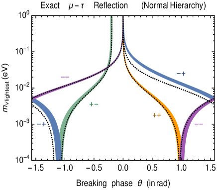
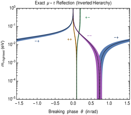
Figure 1: Lightest neutrino mass as a function of the phase $\theta$ (which breaks $\mu-\tau$ permutation symmetry) in the case of exact $\mu-\tau$ reflection symmetry (an example of phase-broken $\mu-\tau$ permutation). Normal (left) and Inverted (right) Hierarchies are considered and the “$++$,” “$+-$”, “$-+$” and “$--$” curves correspond to the different possible values of the Majorana phases ($\eta$=0; $\xi$=0), ($\eta$=0; $\xi=\pi/2)$, ($\eta=\pi/2$; $\xi$=0) or ($\eta=\pi/2$; $\xi=\pi/2$). The curves represent points where the mixing angles $|V_{e3}|$ and $|V_{e2}|$ and the mass differences $\Delta^{2}_{sol}$ and $\Delta^{2}_{atm}$ lie within their 1-$\sigma$ experimental range. Dotted curves represent the simple analytical approximations from Eqs. (69) and (70) where we have used only the central values of experimental data. For Normal Hierachy and very light mass, the phase $\theta$ can only be $\theta_{0}\simeq 1(mod\ \pi)$ or $\theta_{0}\simeq-1.1(mod\ \pi)$, whereas for Inverted Hierarchy we have $\theta_{0}\simeq 0.1(mod\ \pi)$ or $\theta_{0}\simeq 0.7(mod\ \pi)$, (plots are symmetric under $\theta\to\theta-\pi$).

We show graphically these dependencies in figure 1 in which we plot the lightest neutrino mass as a function of the phase parameter $\theta$ for the cases of Normal hierarchy (left panel) and Inverted hierarchy (right panel). The mixing angles $|V_{e3}|$ and $|V_{e2}|$ have been allowed to range in their $1-\sigma$ experimental range and we have also fixed the value of the solar and atmospheric neutrino mass differences to their experimental values, so that we obtain bands of allowed points. We have used the exact expression from Eq.(64), but have also included the approximate expressions from Eqs. (69) and (70) in order to track their validity (dashed curves, obtained using only the central values of the mixing angles). We clearly see that once $|V_{e3}|$, $|V_{e2}|$ and the experimental neutrino mass differences are fixed, the value of $\theta$ determines very precisely the possible lightest neutrino mass. In particular when the lightest mass tends to zero only two values of $\tan(\theta)$ are allowed within the Normal Hierarchy case ($\tan(\theta)\simeq\pm 1.5$) and only two other values are possible for the Inverted Hierarchy case, ($\tan(\theta)\simeq 0.1$ or $\tan(\theta)\simeq 0.9$). Because the function $\tan(\theta)$ has a periodicity of $\pi$ we show only values of $\theta$ between $-\pi/2$ and $\pi/2$.

Note that no other lagrangian parameter enters in these relations showcasing the importance of the phase breaking parameter $\theta$ within exact $\mu$-$\tau$ reflection symmetry.

II.3 Phase broken $\mu$-$\tau$ with $\delta_{CP}=-\pi/2$

In this section we are going to study the particular case where we fix $\delta_{CP}=-\pi/2$, in part guided by the exact analytical results from the previous section and also in part guided by the global fit results from neutrino phenomenology which place $\delta_{CP}$ somewhere around the third quadrant. On the other hand, and unlike the previous section, the Majorana phases can take any value (as long as the model constraints are verified). It turns out that in this limit the analytical results are still quite simple, giving us a further robust understanding of the features of phase broken $\mu-\tau$ symmetry, without having to rely on numerical solutions.

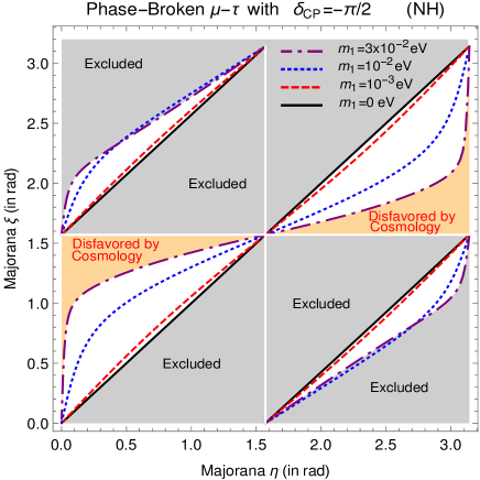
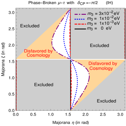
Figure 2: Contours of the lightest neutrino mass as a function of the Majorana phases $\eta$ and $\xi$ within phase-broken $\mu-\tau$ in the limit where the Dirac CP phase in the neutrino sector is $\delta_{CP}=-\pi/2$. The excluded regions on both panels (left for Normal and right for Inverted Hierarchies) represent values of $\eta$ and $\xi$ inconsistent with the sum-rule in eq. (72). Note that because the sum-rule depends on $(2\eta)$ and $(2\xi)$ it is enough to vary their values between $0$ and $\pi$. The regions marked “Disfavored by Cosmology” are regions where the lightest neutrino mass value is too large to evade cosmological constraints cosmology . Also, for the specific values of $0$ and $\pi/2$ for the Majorana phases, the constraint on neutrino masses disappears.

We start with the two constraints $|M_{e\mu}|=|M_{e\tau}|$ and $|M_{\mu\mu}|=|M_{\tau\tau}|$ along with $\delta_{CP}=-\pi/2$. This leads to the equality of the moduli of the elements of the second row and the third row of $V_{PMNS}$, i.e $|V_{\mu i}|=|V_{\tau i}|$ . More specifically we cast the consequences of this particular limit of phase broken $\mu-\tau$ with two simple and exact relations, namely a prediction for $|V_{\mu 3}|$

$$|V_{\mu 3}|=\frac{\sqrt{1-|V_{e3}|^{2}}}{\sqrt{2}}$$ (71)

and the exact sum rule (already given in Eq. (48))

$$|m_{1}||m_{2}|\sin(2\eta)+|m_{1}||m_{3}|\sin(2\xi)+|m_{2}||m_{3}|\sin(2\eta-2\xi)\ =\ 0$$ (72)

in which the majorana phases $\eta$ and $\xi$ are constrained along with the neutrino masses in a very simple way.

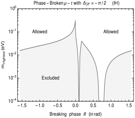
Figure 3: Lightest neutrino mass as a function of the phase $\theta$ (which breaks $\mu-\tau$ permutation symmetry) in the limit where the Dirac CP phase in the neutrino sector is $\delta_{CP}=-\pi/2$, with the Majorana phases $\eta$ and $\xi$ not fixed. The allowed regions represent points in which the mixing angles $|V_{e3}|$ and $|V_{e2}|$ and the mass differences $\Delta^{2}_{sol}$ and $\Delta^{2}_{atm}$ are constrained to lie within their 1-$\sigma$ experimental range. When the lightest neutrino mass is very small, for Normal Hierachy the phase $\theta$ can only be $\theta_{0}\simeq 1(mod\ \pi)$ or $\theta_{0}\simeq-1.1(mod\ \pi)$, whereas for Inverted Hierarchy we have $\theta_{0}\simeq 0.1(mod\ \pi)$ or $\theta_{0}\simeq 0.7(mod\ \pi)$, (plots are symmetric under $\theta\to\theta-\pi$).

Note that for the specific values $0$ or $\pi/2$ for these phases, all the terms of the sum rule vanish and we lose any constraints on the neutrino masses. When the Majorana phases take these values, we obtain the exact $\mu-\tau$ reflection symmetry limit, which can be understood as a particular case of phase broken $\mu-\tau$ symmetry when $\delta_{CP}=\pm\pi/2$. The predictions coming from the sum-rule in eq. (72) are displayed in figure 2, and we observe that vast regions of the $(\eta-\xi)$ parameter space are inconsistent with the sum-rule. Cosmology constraints cosmology also affect importantly the allowed parameter space region as shown in the figure.

Performing a similar scan as in figure 1, we study in figure 3 the relation between the lightest neutrino mass in terms of the phase parameter $\theta$ for the cases of Normal hierarchy (left panel) and Inverted hierarchy (right panel). The mixing angles $|V_{e3}|$ and $|V_{e2}|$ have been allowed to range in their $1-\sigma$ experimental range and we have fixed the value of the solar and atmospheric neutrino mass differences to their central experimental values. In this case we observe that even though $\delta_{CP}$ remains fixed at $=-\pi/2$, the relaxation of the Majorana phases does open an allowed parameter space region that was closed in the $\mu-\tau$ reflection symmetry limit studied in the previous section. We observe two regions, allowed and excluded and we realize that the border of the regions are actually the curves for fixed values of the Majorana phases with $\eta=0$ or $\pi/2$ and $\xi=0$ or $\pi/2$, i.e. the limiting curves correspond to $\mu-\tau$ reflection symmetry points, shown in figure 1.

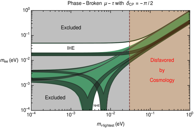
Figure 4: Allowed values (green/darker green) of the effective Majorana mass $m_{ee}$ in terms of the lightest neutrino mass in phase-broken $\mu$-$\tau$ in the limit where the Dirac CP phase in the neutrino sector is fixed to $\delta_{CP}=-\pi/2$, with the Majorana phases $\eta$ and $\xi$ allowed to range within the model theoretical constraints. The dark green regions are points with $\eta$ and $\xi$ fixed to $\pi/2$ or $0$, representing the allowed regions within exact $\mu$-$\tau$ reflection symmetry. The white regions marked “IHE” and “NHE” are excluded due to the phase-broken $\mu$-$\tau$ constraints (in the Inverted and Normal Hierarchy regimes), whereas the gray regions marked “Excluded” violate current experimental constraints on neutrino masses and mixings.

Another interesting phenomenological aspect to consider is the effective Majorana neutrino mass which is given by

$$|m_{ee}|=\Big{|}|m_{1}||V_{e1}|^{2}+|m_{2}||V_{e2}|^{2}e^{2i\eta}+|m_{3}||V_{e3}|^{2}e^{2i(\xi-\delta_{CP})}\Big{|}$$ (73)

New generation and near future experiments comingexperiments will be sensitive to an important region of the allowed parameter space (in the Inverted Hierarchy) so that predictions from phase broken $\mu-\tau$ symmetry could be directly probed.

In figure 4 we show in green/darker green the allowed values of the effective Majorana mass $m_{ee}$ in terms of the lightest neutrino mass in phase-broken $\mu$-$\tau$ for $\delta_{CP}=-\pi/2$, and with the Majorana phases $\eta$ and $\xi$ allowed to range within the phase-broken $\mu-\tau$ constraints. The dark green regions are points where $\eta$ and $\xi$ are fixed to $\pi/2$ or $0$, and so represent the allowed regions for exact $\mu$-$\tau$ reflection symmetry. The upper and lower gray areas are points excluded by current experimental constraints on neutrino masses and mixings, whereas the brown area on the right side represents disfavored points from cosmology cosmology . We observe that broken $\mu-\tau$ scenario puts constraints on two regions of parameter space, shown in white and marked “IHE” (Inverted Hierarchy Exclusion) and “NHE” (Normal Hierarchy Exclusion) representing points excluded by the phase-broken $\mu$-$\tau$ constraints (in the inverted and normal hierarchy regimes).

II.4 Phase broken $\mu$-$\tau$ with specific values for $\delta_{CP}$.

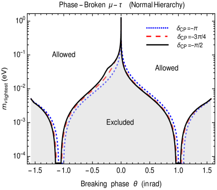
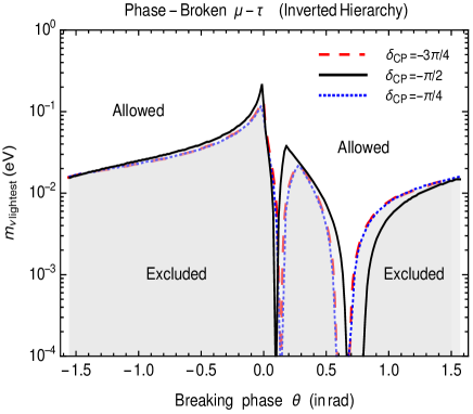
Figure 5: Lightest neutrino mass as a function of the phase $\theta$ (which breaks $\mu-\tau$ permutation symmetry) when the Dirac CP phase in the neutrino sector takes the values $\delta_{CP}=(-\pi/2)$, $(-3\pi/4)$, and $(-\pi)$ for Normal Hierarchy and $\delta_{CP}=(-\pi/4)$, $(-\pi/2)$, and $(-3\pi/4)$ for Inverted Hierarchy. The Majorana phases $\eta$ and $\xi$ are not fixed. The allowed regions represent points in which the mixing angles $|V_{e3}|$ and $|V_{e2}|$ and the mass differences $\Delta^{2}_{sol}$ and $\Delta^{2}_{atm}$ are constrained to lie within their 1-$\sigma$ experimental global fit range.

We finish our overview of the phase broken $\mu-\tau$ symmetry scenario by relaxing the fixed value of $\delta_{CP}$ and cover the range of values prefered by the global fits from neutrino data. We would like to explore here how sensitive are the previous results to relatively small changes in the value of $\delta_{CP}$. Current global fits from experimental data on masses and mixings in the neutrino sector more or less point towards a value of $\delta_{CP}$ roughly located within the range $-\pi\lesssim\delta_{CP}\lesssim-\pi/2$ for Normal Hierarchy, and $-3\pi/4\lesssim\delta_{CP}\lesssim-\pi/4$ for Inverted Hierarchy. We thus wanted to see how the parameter space is constrained within these windows of parameter space.

In figure 5 we show again the dependance of the lightest neutrino mass with respect to the phase-breaking parameter $\theta$ (which breaks the $\mu-\tau$ permutation symmetry) in both the Normal Hierarchy (NH) and Inverted Hierarchy (IH) frameworks. In each case we fix the value of the Dirac phase to $\delta_{CP}=-\pi$, $-3\pi/4$ and -$\pi/2$ (for NH) and $\delta_{CP}=-3\pi/4$, $-\pi/2$ and -$\pi/4$ (for IH). The values for $\delta_{CP}=-\pi/2$ are the same as in figure 3 and the associated points are shown as a continuous black curves. For $\delta_{CP}=-3\pi/4$ we plot the results as red/dashed curves and for $\delta_{CP}=-\pi$ (NH) and $-\pi/4$ (IH) we show the results in blue/dotted curves.

The regions below the curves are excluded by the phase broken $\mu-\tau$ constraints whereas the white regions represent points that are allowed by all theoretical and experimental constraints. We can see that there is not a strong dependence on the value of $\delta_{CP}$, at least within this window, so that the results from the previous section are quite typical within this extended parameter space.

We still observe that for very light neutrino mass, the phase breaking phase $\theta$ is extremely constrained. In the NH case its values must be $\theta_{0}\simeq 1$ $(mod\ \pi)$ or $\theta_{0}\simeq-1.1$ $(mod\ \pi)$, with essentially no dependance on the value of $\delta_{CP}$ or the Majorana phases $\eta$ and $\xi$. For Inverted Hierarchy we have $\theta_{0}\simeq 0.1$ $(mod\ \pi)$ or $\theta_{0}\simeq 0.7$-$0.8$ $(mod\ \pi)$, this time with a mild dependance on $\delta_{CP}$, but no dependance on the Majorana phases $\eta$ and $\xi$.

We can prove analytically these features by analyzing the phase broken $\mu-\tau$ constraints in the limits $m_{1}=0$ (NH) or $m_{3}=0$ (IH), and performing an expansion in $|V_{e3}|$ and the mass ratio parameter $\displaystyle r=\frac{\Delta^{2}_{sol}}{\Delta^{2}_{atm}}$. We find, to lowest order, the analytical expression

$$\tan{\theta}\simeq\pm\frac{2\sqrt{r}\sqrt{1-|V_{e2}|^{2}}|V_{e2}||V_{e3}|}{r|V_{e2}|^{2}(1-|V_{e2}|^{2})-|V_{e3}|^{2}}$$ (74)

for NH, and for IH we obtain two possible values of the phase breaking parameter

$$\tan(\theta) \simeq -\frac{r|V_{e1}||V_{e2}|}{|V_{e3}|}\sin(\delta)$$ (75)

or

$$\tan(\theta) \simeq -\frac{\left[1-4|V_{e1}|^{2}|V_{e2}|^{2}\cos^{2}(\delta)\right]|V_{e3}|\sin(\delta)}{|V_{e1}||V_{e2}|\left[1-2|V_{e2}|^{2}\right]}$$ (76)

It is easy to check that using the experimental values for $r$, $|V_{e2}|$ and $|V_{e3}|$, and including the appropriate values of $\delta_{CP}$, one reproduces the values of $\theta$ located at the “throats” of the numerical curves of Figure 5.

We note however that these expressions are completely general predictions of the phase-broken $\mu-\tau$ paradigm, for any value of $\delta_{CP}$ as long as we are in the limit of a massless (or vey light) lightest neutrino. It is quite non-trivial that the dependance on the Majorana phases disappears in the limit of vanishing mass for the lightest neutrino.

III Conclusions

In this paper we have considered deviations from the usual $\mu$-$\tau$ symmetry framework by adding general phases to a $\mu$-$\tau$ symmetric neutrino mass matrix. We called the obtained framework phase-broken $\mu$-$\tau$ symmetry and studied its general predictions.

As a general result of the setup, the atmospheric mixing element $|V_{\mu 3}|^{2}$ is predicted to be less than a half ($|V_{\mu 3}|^{2}<\frac{1}{2}$), with the deviation set by $|V_{e3}|^{2}/2$. Also a different value for $|V_{\mu 3}|$ is predicted for the cases of NH and IH mass orderings, although the difference is numerically very small and thus will be quite challenging to test experimentally.

One example of our framework turns out to be a very well studied version of $\mu$-$\tau$ symmetry, namely the $\mu$-$\tau$ reflection symmetry. Indeed the $\mu$-$\tau$ reflection symmetry can be understood as a phase-broken $\mu$-$\tau$ permutation symmetry, with additional constraints on the mass matrix elements (namely that the only new phase lies in the phase-breaking phase $\theta$). With this point of view we were able to extract new relations associated to $\mu$-$\tau$ reflection symmetry (to our knowledge) and in particular we obtained analytical expressions of the mixing angle $|V_{e3}|$ in terms of masses and mixing, involving only the phase breaking parameter $\theta$ out of the Lagrangian parameters.

We then studied relaxations of the $\mu$-$\tau$ reflection symmetry within the point of view of phase-broken $\mu$-$\tau$ symmetry, by scanning the paramater space staying in regions where the value of the Dirac CP phase $\delta_{CP}$ is close to $-\pi/2$.

As a general feature in this region of parameter space we observe that in order to allow for a very light neutrino mass, the model requires the phase breaking parameter to have precise values (two different allowed values for Normal Hierarchy and two other for Inverted Hierarchy). Heavier lightest neutrino masses will relax the constraint, but the model still showcases a direct sensitivity to a single lagrangian parameter, the phase $\theta$.

IV Acknowledgments

E.I. Lashin and N. Chamoun acknowledge support from ICTP-Associate program. N.C. acknowledges support of the Alexander von Humboldt Foundation and is grateful for the kind hospitality of the Bethe Center for Theoretical Physics at Bonn University. E.L.’s work was partially supported by the STDF project 37272. S. Nasri thanks the ICTP where part of this work was carried out. M.Toharia would like to thank FRQNT for partial financial support under grant numbers PRCC-191578 and PRC-290000.

V Appendix: Analytical Treatment of phase-broken $\mu-\tau$.

Using Eqs. (16)-(42), the constraints $|M_{e\mu}|=|M_{e\tau}|$ and $|M_{\mu\mu}|=|M_{\tau\tau}|$ can be recast as

$$M_{\mu\mu} = e^{2i(\theta-2\sigma)}M_{\tau\tau}$$ (77)

$$M_{e\mu} = e^{2i(\theta-\sigma)}M_{e\tau}.$$ (78)

The two complex equations (77) and (78) of “phase breaking” $\mu-\tau$ symmetry represent two real constraint equations among the neutrino sector physical parameters, and two real equations involving the phase breaking parameters $\theta$ and $\sigma$ in terms of the neutrino physical parameters. We cast them as

$$(|M_{\mu\mu}|^{2}-|M_{\tau\tau}|^{2}) = (|M_{e\tau}|^{2}-|M_{e\mu}|^{2})\ \ \ \ \ \ (``H_{22}=H_{33}\ equation^{\prime\prime})\$$ (79)

$$|M_{e\mu}|^{2} = |M_{e\tau}|^{2}\ \ \ \ \ \ \ \ \ \ \ \ (``sum-rule\ equation^{\prime\prime})$$ (80)

$$e^{2i\theta} = \left(\frac{M_{\tau\tau}M^{2}_{e\mu}}{M_{\mu\mu}M^{2}_{e\tau}}\right)\ \ \ \ \ \ \ \ \ \ \ \ (``\theta\ \ equation^{\prime\prime})$$ (81)

$$e^{2i\sigma} = \left(\frac{M_{\tau\tau}M_{e\mu}}{M_{\mu\mu}M_{e\tau}}\right)\ \ \ \ \ \ \ \ \ \ \ \ (``\sigma\ \ equation^{\prime\prime})$$ (82)

where the matrix $H$ is defined as $H_{\nu}=M_{\nu}M_{\nu}^{\dagger}$. The “$\sigma$ equation” involves the unphysical phase $\sigma$ as well as the unphysical diagonalization phases $\gamma_{2}$ and $\gamma_{3}$ and thus does not constrain directly any physical parameter.

However the other three equations have direct phenomenological effect on the physical parameters. Note that $\theta$ is the only parameter coming from the original neutrino mass matrix and from Eq. (81) we can extract its value once we fix all the observable parameters in the neutrino sector, i.e. $|V_{e3}|,|V_{\mu 3}|,|V_{e2}|,\delta,\eta,\xi,|m_{1}|,|m_{2}|$ and $|m_{3}|$.

Note that Eqs. (79) and (80) represent constraints among the physical parameters of the neutrino sector. We choose to eliminate $|V_{\mu 3}|$ using Eq. (79) (which we refer to as the “$H_{22}=H_{33}$ equation”) and $\eta$ using equation (80) (which we call the “$sum-rule$ equation”) and in particular we obtain the dependencies $|V_{\mu 3}|\equiv f(|V_{e3}|,|V_{e2}|,\delta,|m_{1}|,|m_{2}|,|m_{3}|)$ and $\eta\equiv g(|V_{e3}|,|V_{e2}|,\delta,\xi,|m_{1}|,|m_{2}|,|m_{3}|)$. From these, the phase breaking parameter $\theta$ has a dependency as $\theta\equiv h(|V_{e3}|,|V_{e2}|,\delta,\xi,|m_{1}|,|m_{2}|,|m_{3}|)$ and so fixing $|V_{e3}|,|V_{e2}|,\delta,|m_{2}|,|m_{3}|$ to their experimental values gives us a simpler parameter dependency $\theta\equiv h(\xi,|m_{lightest}|)$. Before going into details on the main constraint equations from this setp, we will show a revealing table with the counting of parameters in the different implementations of $\mu-\tau$ symmetry discussed here.

Setup	$M_{\nu}$	$D_{\nu}$	$U_{\nu}$	$V_{\mbox{\tiny{PMNS}}}$	$P_{L}$
		$\mbox{diag}(|m_{1}|,|m_{2}|,|m_{3}|)$	$U^{\dagger}_{\nu}M_{\nu}U^{*}_{\nu}=D_{\nu}$	$U_{\nu}=P_{L}V_{\mbox{\tiny{PMNS}}}$
General case	$12$	$3$	$9$	$6$	$3$
Exact $\mu-\tau$ permutation	$8$	$3$	$5$	$3$	$2$
Exact $\mu-\tau$ reflection	6	$3$	$3$	$2$	$1$
Phase broken $\mu-\tau$	$10$	$3$	$7$	$4$	$3$

Table 1: Number of real free parameters for the neutrino mass related matrices, in the basis where the charged lepton mass matrix is diagonal and real, for different $\mu-\tau$ symmetry implementations.

V.1 The “$H_{22}=H_{33}$” equation

Let us begin with the general case which corresponds to $|M_{e\mu}|=|M_{e\tau}|$ and $|M_{\mu\mu}|=|M_{\tau\tau}|$. These two equations can be combined to give the constraint

$$(|M_{\mu\mu}|^{2}-|M_{\tau\tau}|^{2}) = (|M_{e\tau}|^{2}-|M_{e\mu}|^{2})$$ (83)

We then realize that at the level of the hermitian matrix $H_{\nu}=M_{\nu}M_{\nu}^{\dagger}$, the two diagonal elements $H_{22}$ and $H_{33}$ are given by $H_{22}=|M_{e\mu}|^{2}+|M_{\mu\mu}|^{2}+|M_{\mu\tau}|^{2}$ and $H_{33}=|M_{e\tau}|^{2}+|M_{\mu\tau}|^{2}+|M_{\tau\tau}|^{2}$. We see that Eq. (83) is equivalent to enforcing $H_{22}=H_{33}$ at the level of the hermitian matrix $H_{\nu}$. Note that working with the elements of $H_{\nu}$ has the benefit of removing the dependance on the Majorana phases $\eta$ and $\xi$. We have in particular

$$H_{22} = |m_{1}|^{2}+(|m_{2}|^{2}-|m_{1}|^{2})|V_{\mu 2}|^{2}+(|m_{3}|^{2}-|m_{1}|^{2})|V_{\mu 3}|^{2}$$ (84)

$$H_{33} = |m_{1}|^{2}+(|m_{2}|^{2}-|m_{1}|^{2})|V_{\tau 2}|^{2}+(|m_{3}|^{2}-|m_{1}|^{2})|V_{\tau 3}|^{2}$$ (85)

Imposing the condition $H_{22}=H_{33}$ and using the definitions for $V_{\mu 2}$ and $V_{\tau 2}$ from Eqs. (34) and (36) we obtain the expression

$$X\left[(1-|V_{e3}|^{2})^{2}-r[|V_{e1}|^{2}-|V_{e2}|^{2}|V_{e3}|^{2}]\right]=rD\cos(\delta_{CP})$$ (86)

for a normal neutrino mass spectrum ($\Delta_{atm}^{2}=|m_{3}|^{2}-|m_{1}|^{2}$) and

$$X\left[(1-|V_{e3}|^{2})^{2}+r[|V_{e1}|^{2}-|V_{e2}|^{2}|V_{e3}|^{2}]\right]=-rD\cos(\delta_{CP})$$ (87)

for an inverted spectrum ($\Delta_{atm}^{2}=|m_{1}|^{2}-|m_{3}|^{2}$).

In both expressions $\Delta_{sol}^{2}=|m_{2}|^{2}-|m_{1}|^{2}$ and $r=\frac{\Delta_{sol}^{2}}{\Delta_{atm}^{2}}$, and we have defined

$$X = |V_{\tau 3}|^{2}-|V_{\mu 3}|^{2}$$ (88)

$$D = 4|V_{e1}||V_{e2}||V_{e3}||V_{\mu 3}||V_{\tau 3}|$$ (89)

in order to simplify the notation. From these equations one can obtain an exact expression for the atmospheric neutrino mixing element given by

$$|V_{\mu 3}|^{2}_{NH}=\frac{1}{2}\left(1-|V_{e3}|^{2}\right)\left(1-\frac{\varepsilon_{N}}{\sqrt{1+\varepsilon_{N}^{2}}}\right)$$ (90)

in the normal hierarchy regime, and where we have defined the (small) parameter $\varepsilon_{N}$ as

$$\varepsilon_{N}=\frac{2r|V_{e1}||V_{e2}||V_{e3}|\cos(\delta_{CP})}{(1-|V_{e3}|^{2})^{2}-r[|V_{e1}|^{2}-|V_{e2}|^{2}|V_{e3}|^{2}]}.$$ (91)

For the inverted hierarchy regime, we obtain

$$|V_{\mu 3}|^{2}_{IH}=\frac{1}{2}\left(1-|V_{e3}|^{2}\right)\left(1+\frac{\varepsilon_{I}}{\sqrt{1+\varepsilon_{I}^{2}}}\right)$$ (92)

and again we have defined the (small) parameter $\varepsilon_{I}$ as

$$\varepsilon_{I}=\frac{2r|V_{e1}||V_{e2}||V_{e3}|\cos(\delta_{CP})}{(1-|V_{e3}|^{2})^{2}+r[|V_{e1}|^{2}-|V_{e2}|^{2}|V_{e3}|^{2}]}.$$ (93)

By performing an expansion in powers of $\varepsilon_{N}$ and $\varepsilon_{I}$ and keeping the lowest terms one trivially reproduces the expressions given in the main text in Eqs. (43) and (44).

V.2 The “Sum-Rule” Equation

To extract useful information on the ${\cal CP}$ violating phase $\delta$, it is more convenient to express the second constraint, $|M_{e\mu}|^{2}=|M_{e\tau}|^{2}$ as

$$X\left[F_{1}+|V_{e3}|^{2}F_{2}\right]+D\left[\tilde{K}_{1}\cos(\delta)+\tilde{K}_{2}\sin(\delta)\right]=0$$ (94)

where we have defined

$$F_{1} = |V_{e1}|^{2}|V_{e2}|^{2}\left[|m_{1}|^{2}+|m_{2}|^{2}-2|m_{1}||m_{2}|\cos(2\eta)\right]$$ (95)

$$F_{2} = 2|m_{1}||m_{3}||V_{e1}|^{2}(1-|V_{e3}|^{2})\cos(2\xi-2\delta)+2|m_{2}||m_{3}||V_{e2}|^{2}(1-|V_{e3}|^{2})\cos(2\eta-2\xi+2\delta)$$ (96)

$$-2|m_{1}||m_{2}||V_{e1}|^{2}|V_{e2}|^{2}\cos(2\eta)-|m_{1}|^{2}|V_{e1}|^{4}-|m_{2}|^{2}|V_{e2}|^{4}-|m_{3}|^{2}(1-|V_{e3}|^{2})^{2}$$

$$\tilde{K}_{1} = |m_{2}|^{2}|V_{e2}|^{2}-|m_{1}|^{2}|V_{e1}|^{2}-2|m_{1}||m_{2}||V_{e2}|^{2}\cos(2\eta)$$ (97)

$$+\left[|m_{1}||m_{2}|\cos(2\eta)+|m_{1}||m_{3}|\cos(2\xi)-|m_{2}||m_{3}|\cos(2\eta-2\xi)\right](1-|V_{e3}|^{2})$$

$$\tilde{K}_{2} = \left[|m_{1}||m_{2}|\sin(2\eta)+|m_{1}||m_{3}|\sin(2\xi)+|m_{2}||m_{3}|\sin(2\eta-2\xi)\right](1-|V_{e3}|^{2}).$$ (98)

Injecting the value of the parameter $X$ obtained from the “$H_{22}=H_{33}$ equation” (Eqs. (86) and (87) ) we can eliminate the dependance on $|V_{\mu 3}|$ and obtain, for the normal mass hierarchy,

$$\cot(\delta)_{NH}=-\frac{(1-|V_{e3}|^{2})^{2}(1-rZ)\tilde{K}_{2}}{(1-|V_{e3}|^{2})^{2}(1-rZ)\tilde{K}_{1}+r\left[F_{1}+|V_{e3}|^{2}F_{2}\right]},$$ (99)

and for the inverted mass hierarchy,

$$\cot(\delta)_{IH}=-\frac{(1-|V_{e3}|^{2})^{2}(1+rZ)\tilde{K}_{2}}{(1-|V_{e3}|^{2})^{2}(1+rZ)\tilde{K}_{1}-r\left[F_{1}+|V_{e3}|^{2}F_{2}\right]}$$ (100)

where,

$$Z = \frac{|V_{e1}|^{2}-|V_{e2}|^{2}|V_{e3}|^{2}}{(1-|V_{e3}|^{2})^{2}}.$$ (101)

The above equations depend only on the physical parameters $|m_{1}|$, $|m_{2}|$, $|m_{3}|$, $\delta_{CP}$, $\xi$, $\eta$, $|V_{e2}|$ and $|V_{e3}|$. Note also that the expression $F_{2}$ contains some further dependence on $\delta_{CP}$. However, if we drop terms proportional to $r$ and $|V_{e3}|^{2}$, then we obtain a simple relation between $\cot(\delta)$ and the neutrino masses, the $|V_{ij}|^{2}$ and the two Majorana ${\cal CP}$ violating phases $\eta$ and $\xi$

$$\cot(\delta)=-\frac{K_{2}}{K_{1}}\ \ +\ {\cal O}(r,|V_{e3}|^{2})$$ (102)

valid for both normal and inverted mass orderings and with $K_{i}$ (without tilde) defined as

$$K_{1} = |m_{2}|^{2}|V_{e2}|^{2}-|m_{1}|^{2}(1-|V_{e2}|^{2})+(1-2|V_{e2}|^{2})|m_{1}||m_{2}|\cos(2\eta)$$ (103)

$$\ +|m_{1}||m_{3}|\cos(2\xi)-|m_{2}||m_{3}|\cos(2\eta-2\xi)$$

$$K_{2} = |m_{1}||m_{2}|\sin(2\eta)+|m_{1}||m_{3}|\sin(2\xi)+|m_{2}||m_{3}|\sin(2\eta-2\xi).$$ (104)

V.3 The “$\theta$” equation

From the phase-broken $\mu-\tau$ symmetry constraints we can obtain an expression of $\tan(\theta)$ as

$$\tan(\theta) = \frac{Im\left[M_{\mu\mu}^{*}M_{\tau\tau}(M_{e\mu}M_{e\tau}^{*})^{2}\right]}{|M_{\mu\mu}|^{2}|M_{e\mu}|^{4}+Re\left[M_{\mu\mu}^{*}M_{\tau\tau}(M_{e\mu}M_{e\tau}^{*})^{2}\right]}$$ (105)

where the $M_{ij}$ are defined in Eqs. (38)-(41). The exact expression of $\tan(\theta)$ in terms of masses and mixing angles is long and not very revealing. However, the approximate relations keeping only the lowest terms in $|V_{e3}|$ and $r$, and in the special limits of $|m_{1}|=0$ and $|m_{3}|=0$ are simple and match the numerical results obtained using the exact expression.

• In the case of $|m_{1}|=0$ and expanding in $|V_{e3}|$ and $r$ we have, to lowest order,

  $$\tan(\theta)\simeq\frac{2\sqrt{r}|V_{e1}||V_{e2}||V_{e3}|}{\left[r|V_{e1}|^{2}|V_{e2}|^{2}-|V_{e3}|^{2}\right]}\sin(2\eta-2\xi+\delta)$$ (106)

  However we still need to implement in the above expression the condition coming from the sum rule constraint from Eq (99), which in this limit can be written as,

  $$\sin(2\eta-2\xi+\delta) = \pm\left[1-\frac{r}{2}|V_{e2}|^{4}\cos^{2}(\delta)\right]$$ (107)

  Injecting the above value in the expression of $\tan(\theta)$, we finally obtain

  $$\tan(\theta)\simeq\pm\frac{2\sqrt{r}|V_{e1}||V_{e2}||V_{e3}|}{\left[r|V_{e1}|^{2}|V_{e2}|^{2}-|V_{e3}|^{2}\right]}$$ (108)

• The case $|m_{3}|=0$ is more subtle. Again, for small $|V_{e3}|$, we obtain,

  $$\tan(\theta)=\frac{S}{2R}+\frac{Q}{P}\ +\ {\cal O}(|V_{e3}|^{3})$$ (109)

  where,

  $$S = -2|V_{e1}||V_{e2}||V_{e3}|\sin(\delta)\left(4(1-2|V_{e2}|^{2})\sin^{2}(\eta)+r\right)$$ (110)

  $$Q = S+4r|V_{e1}||V_{e2}||V_{e3}|\sin(\delta)$$ (111)

  $$P = 8|V_{e2}|^{2}(1-|V_{e2}|^{2})\sin^{2}(\eta)-2\left[1+4|V_{e2}|^{2}\sin^{2}(\eta)\right]|V_{e3}|^{2}$$ (112)

  $$R = 1-4|V_{e2}|^{2}(1-|V_{e2}|^{2})\sin^{2}(\eta)-r(1-|V_{e2}|^{2})-4\left[\cos^{2}(\eta)-\cos^{2}(\delta)\cos(2\eta)\right]|V_{e3}|^{2}$$

  $$-4\sin^{2}(\eta)|V_{e2}|^{2}\left[1-2|V_{e2}|^{2}+4(1-|V_{e2}|^{2})\sin^{2}(\delta)\right]|V_{e3}|^{2}+2(1-2|V_{e2}|^{2})\sin(2\delta)\sin(2\eta)|V_{e3}|^{2}.$$

  Two different limits for $\eta$ stand out from the previous expression.

  • For $\sin(\eta)\ll|V_{e3}|$, the expression simplifies to

    $$\tan(\theta) \simeq -\frac{r|V_{e1}||V_{e2}|}{|V_{e3}|}\sin(\delta)$$ (114)

  • For $\sin(\eta)\gg|V_{e3}|$, the expression becomes

    $$\tan(\theta) \simeq -\frac{\left[1-4|V_{e1}|^{2}|V_{e2}|^{2}\cos^{2}(\delta)\right]|V_{e3}|\sin(\delta)}{|V_{e1}||V_{e2}|\left[1-2|V_{e2}|^{2}\right]}$$ (115)

  • For $\sin(\eta)\simeq{\cal O}(|V_{e3}|)$ the analytical expression is cumbersome and not specially revealing.

References

- (1) [T2K Collaboration], Y. Abe et al., Phys. Rev. Lett. 107, 041801 (2011).
- (2) [Double Chooz Collaboration], Y. Abe et al., Phys. Rev. Lett. 108, 131801 (2012.
- (3) [RENO collaboration], J. Ahn et al., Phys. Rev. Lett. 108, 191802 (2012).
- (4) [Daya Bay Collaboration], F. An et al., Phys. Rev. Lett. 108, 171803 (2012).
- (5) T. Fukuyama and H. Nishiura, hep-ph/9702253; R. N. Mohapatra and S. Nussinov, Phys. Rev. D 60, 013002 (1999); C. S. Lam, Phys. Lett. B 507, 214 (2001); T. Kitabayashi and M. Yasue, Phys. Rev. D 67, 015006 (2003).
- (6) P. F. Harrison and W. G. Scott, Phys. Lett. B 547, 219 (2002).
- (7) W. Grimus and L. Lavoura, JHEP 0107, 045 (2001); W. Grimus and L. Lavoura, Phys. Lett. B 572, 189 (2003); Y. Koide, Phys. Rev. D 69, 093001 (2004); R. N. Mohapatra, JHEP 0410, 027 (2004).
- (8) G. Altarelli and F. Feruglio, Rev. Mod. Phys. 82, 2701 (2010).
- (9) E. Ma and M. Raidal, Phys. Rev. Lett. 87, 011802 (2001); W. Grimus and L. Lavoura, JHEP 0107, 045 (2001); E. Ma, Phys. Rev. D 66, 117301 (2002); R. N. Mohapatra and S. Nasri, Phys. Rev. D 71, 033001 (2005); R. N. Mohapatra and W. Rodejohann, Phys. Rev. D 72, 053001 (2005); R. N. Mohapatra, S. Nasri and H. -B. Yu, Phys. Lett. B 615, 231 (2005); S. Nasri, Int. J. Mod. Phys. A 20, 6258 (2005); T. Kitabayashi and M. Yasue, Phys. Lett. B 621, 133 (2005); S. Choubey and W. Rodejohann, Eur. Phys. J. C 40, 259 (2005); R. N. Mohapatra, S. Nasri and H. B. Yu, Phys. Lett. B 636, 114 (2006); R. N. Mohapatra, S. Nasri and H. B. Yu, Phys. Lett. B 639, 318 (2006); Z. -z. Xing, H. Zhang and S. Zhou, Phys. Lett. B 641, 189 (2006); T. Ota and W. Rodejohann, Phys. Lett. B 639, 322 (2006); Y. H. Ahn, S. K. Kang, C. S. Kim and J. Lee, Phys. Rev. D 73, 093005 (2006); I. Aizawa and M. Yasue, Phys. Rev. D 73, 015002 (2006); K. Fuki and M. Yasue, Phys. Rev. D 73, 055014 (2006); K. Fuki and M. Yasue, R. Jora, S. Nasri and J. Schechter, Int. J. Mod. Phys. A 21, 5875 (2006), Nucl. Phys. B 783, 31 (2007); B. Adhikary, A. Ghosal and P. Roy, JHEP 0910 (2009) 040; B. Adhikary, A. Ghosal and P. Roy, JHEP 0910, 040 (2009); Z. z. Xing and Y. L. Zhou, Phys. Lett. B 693, 584 (2010); R. Jora, J. Schechter and M. Naeem Shahid, Phys. Rev. D 80, 093007 (2009) [Erratum-ibid. D 82, 079902 (2010)]; S. -F. Ge, H. -J. He and F. -R. Yin, JCAP 1005, 017 (2010); I. de Medeiros Varzielas, R. González Felipe and H. Serodio, Phys. Rev. D 83, 033007 (2011); H. -J. He and F. -R. Yin, Phys. Rev. D 84, 033009 (2011); Y. H. Ahn, H. Y. Cheng, S. Oh, Phys. Lett. B 715, 203 (2012); H. -J. He and X. -J. Xu, Phys. Rev. D 86, 111301 (2012); S. Gupta, A. S. Joshipura and K. M. Patel, JHEP 1309, 035 (2013); B. Adhikary, M. Chakraborty and A. Ghosal, JHEP 1310, 043 (2013); B. Adhikary, A. Ghosal and P. Roy, Int. J. Mod. Phys. A 28, no. 24, 1350118 (2013).
- (10) P. F. de Salas, D. V. Forero, C. A. Ternes, M. Tortola and J. W. F. Valle, Phys. Lett. B 782, 633 (2018) doi:10.1016/j.physletb.2018.06.019 [arXiv:1708.01186 [hep-ph]].
- (11) I. Esteban, M. C. Gonzalez-Garcia, A. Hernandez-Cabezudo, M. Maltoni and T. Schwetz, JHEP 1901, 106 (2019) doi:10.1007/JHEP01(2019)106 [arXiv:1811.05487 [hep-ph]].
- (12) R. N. Mohapatra and W. Rodejohann, Phys. Rev. D 72, 053001 (2005) doi:10.1103/PhysRevD.72.053001 [hep-ph/0507312].
- (13) M. H. Rahat, P. Ramond and B. Xu, Phys. Rev. D 98, no. 5, 055030 (2018) [arXiv:1805.10684 [hep-ph]].
- (14) P. F. Harrison, D. H. Perkins and W. G. Scott, Phys. Lett. B 530, 167 (2002) [hep-ph/0202074].
- (15) W. Grimus and L. Lavoura, Fortschritte der Physik, 61(4-5); 535545, Oct 2012
- (16) E. I. Lashin, N. Chamoun, C. Hamzaoui and S. Nasri, PRD 89, 093004 (2014), arXiv: 1311.5869 [hep-ph]
- (17) W. Grimus, A.S. Joshipura, S. Kaneko, L. Lavoura, H. Sawanaka, M. Tani- moto, Nucl. Phys. B713: 151-172, 2005. arXiv:hep-ph/0408123.
- (18) W. Grimus and L. Lavoura, Phys. Lett. B 579, 113 (2004) [hep-ph/0305309];
- (19) P. Chen, G. J. Ding, F. Gonzalez-Canales and J. W. F. Valle, Phys. Lett. B 753, 644 (2016) [arXiv:1512.01551 [hep-ph]].
- (20) Z. z. Xing and Z. h. Zhao, Rept. Prog. Phys. 79, no. 7, 076201 (2016) [arXiv:1512.04207 [hep-ph]]; Z. z. Xing, Phys. Rept. 854, 1-147 (2020) [arXiv:1909.09610 [hep-ph]].
- (21) H. J. He, W. Rodejohann and X. J. Xu, Phys. Lett. B 751, 586 (2015) [arXiv:1507.03541 [hep-ph]]; A. S. Joshipura and K. M. Patel, Phys. Lett. B 749, 159 (2015) [arXiv:1507.01235 [hep-ph]]; W. Rodejohann and X. J. Xu, Phys. Rev. D 96, no. 5, 055039 (2017) [arXiv:1705.02027 [hep-ph]]; C. C. Nishi, B. L. Sánchez-Vega and G. Souza Silva, JHEP 1809, 042 (2018) [arXiv:1806.07412 [hep-ph]]; S. F. King and C. C. Nishi, Phys. Lett. B 785, 391 (2018) [arXiv:1807.00023 [hep-ph]]; N. Nath, Phys. Rev. D 98, no. 7, 075015 (2018) [arXiv:1805.05823 [hep-ph]]; K. Chakraborty, K. N. Deepthi, S. Goswami, A. S. Joshipura and N. Nath, Phys. Rev. D 98, no. 7, 075031 (2018) [arXiv:1804.02022 [hep-ph]]; Z. h. Zhao, Nucl. Phys. B 935, 129 (2018) [arXiv:1803.04603 [hep-ph]]; G. y. Huang, Z. z. Xing and J. y. Zhu, Chin. Phys. C 42, no. 12, 123108 (2018) [arXiv:1806.06640 [hep-ph]]; N. Nath, R. Srivastava and J. W. F. Valle, Phys. Rev. D 99, no. 7, 075005 (2019) [arXiv:1811.07040 [hep-ph]].
- (22) R. Acciarri et al. (DUNE), (2015), arXiv:1512.06148 [physics.ins-det] ; K. Abe et al. (T2K), Phys. Rev. Lett. 118, 151801 (2017), arXiv:1701.00432 [hep-ex]; A. Radovic et al. (NOvA) (2018) talk given at the Fermilab, January 2018, USA, http://nova-docdb.fnal.gov/cgi-bin/ShowDocument?docid=25938; M. J. Dolinski, A. W. P. Poon and W. Rodejohann, Ann. Rev. Nucl. Part. Sci. 69, 219-251 (2019), [arXiv:1902.04097 [nucl-ex]].
- (23) N. Aghanim et al. [Planck], Astron. Astrophys. 641, A6 (2020), [arXiv:1807.06209 [astro-ph.CO]].