Temporal Ordered Clustering in Dynamic Networks: Unsupervised and Semi-supervised Learning Algorithms

Abstract

In temporal ordered clustering, given a single snapshot of a dynamic network in which nodes arrive at distinct time instants, we aim at partitioning its nodes into $K$ ordered clusters $\mathcal{C}_{1}\prec\cdots\prec\mathcal{C}_{K}$ such that for $i<j$, nodes in cluster $\mathcal{C}_{i}$ arrived before nodes in cluster $\mathcal{C}_{j}$, with $K$ being a data-driven parameter and not known upfront. Such a problem is of considerable significance in many applications ranging from tracking the expansion of fake news to mapping the spread of information. We first formulate our problem for a general dynamic graph, and propose an integer programming framework that finds the optimal clustering, represented as a strict partial order set, achieving the best precision (i.e., fraction of successfully ordered node pairs) for a fixed density (i.e., fraction of comparable node pairs). We then develop a sequential importance procedure and design unsupervised and semi-supervised algorithms to find temporal ordered clusters that efficiently approximate the optimal solution. To illustrate the techniques, we apply our methods to the vertex copying (duplication-divergence) model which exhibits some edge-case challenges in inferring the clusters as compared to other network models. Finally, we validate the performance of the proposed algorithms on synthetic and real-world networks.

I Introduction

The clustering of nodes is a classic problem in networks. In its typical form in static networks, it finds communities where methods like spectral clustering, modularity maximization, minimum-cut method, and hierarchical clustering are commonly used [1].

However, in dynamic networks that grow over time with nodes or edges getting added or deleted, a criteria of clustering based on its temporal characteristics finds significant relevance in practice since it helps us to study the existence of certain network structures and their future behavior. One approach to reason about the history of dynamic networks via clustering is guided by the problem of node labeling according to their arrival order when only the structure of the final snapshot of the network is provided. The availability of merely structure means that either we are given an unlabeled graph or the current node labels do not present any historical information. As it turns out, in many real-world networks and graph models, it is impossible to find a complete order of arrival of nodes due to a large number of symmetries inherent in the graph [2, 3]. Figure 1 shows an example. In such cases, it is essential to classify nodes that are indistinguishable themselves in terms of arrival order into clusters $\{\mathcal{C}_{i}\}$. Furthermore, the formed clusters also will be ordered as $\mathcal{C}_{1}\prec\mathcal{C}_{2}\prec\cdots$ so that for any $i<j$, all the nodes in the cluster $\mathcal{C}_{i}$ are estimated to be arrived earlier than all the nodes in the cluster $\mathcal{C}_{j}$, and all the nodes inside each cluster are considered to be identical in arrival order. We call such a clustering scheme as temporal ordered clustering.

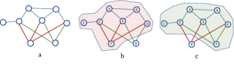
Figure 1: Example showing how temporal clustering arises: a) the input graph without labels. b) and c) arbitrary labellings of arrival order with $1$ representing the earliest arrival and $8$ for the latest arrival. In b) and c), the last two arrived nodes $7$ and $8$ have the same set of neighbors. If we simulate the process of evolution starting from node $1$, we observe that graphs in b) and c) at time $7$ (i.e., with nodes $1-7$) are identical. Thus, nodes $7$ and $8$ in b) and c) are indistinguishable as to which arrived early between them (this observation holds for any labeling on the input graph), and the nodes behind these two labels are part of a temporal cluster.

Temporal ordered clustering is related to many applications in practice. For example in online social networks, it can be useful to disseminate specific information or advertisements targeted at nodes that arrived around the same time. In biological networks, it identifies the evolution of biomolecules in the network and helps in predicting early proteins that are known to be preferentially implicated in cancers and other diseases [4]. In rumor or epidemic networks, temporal ordered clustering can assist in identifying the sources and carriers of false information.

Our contributions.

• We provide a general framework and derive an optimization problem for finding temporal ordered clusters in dynamic networks when only the final snapshot of its evolution is provided. Due to high computational complexity involved in solving it, we reformulate the problem in terms of partial orders – for any node pairs $(u,v)$, a partial order $\sigma$ defines an order $u<_{\sigma}v$ in which node $u$ is specified to be arrived earlier than node $v$. Such a partial order naturally translates into clusters of nodes and introduces an order among them. Both the optimization problems depend on the knowledge of the probabilistic evolution of the graph model and the probability that any node $u$ is older than any other node $v$, denoted as $p_{u,v}$. We then design a sequential importance sampling algorithm to estimate $p_{u,v}$ for any general graph model, and prove its convergence. The solution to a linear programming relaxation of the original optimization problem, with coefficients as estimated $p_{u,v}$, presents an upper bound on the clustering quality.

• In the case of large networks, when the complexity for solving the original optimization is higher, approximate solutions, which directly make use of the estimated $p_{u,v}$s, are developed. Moreover, when some information about the node-pair orders are available, we develop semi-supervised techniques that exploit the graph structure to improve estimation precision. We observe that the use of semi-supervised learning enhances the estimated values of $p_{u,v}$ quickly even with a small percentage of labeled data.

• In the second part of the paper, as an application of the proposed general technique, we focus on duplication-divergence or vertex copying dynamic network model (DD-model) in which, informally, a new node copies the edges of a randomly selected existing node and retains them with a certain probability, and also makes random connections to the remaining nodes (see Section V-A for details). The DD-model poses unique challenges for temporal ordered clustering in comparison with other graph models because of the features listed below:

  • Non-equiprobable large number of permutations: In many of the graph models including the preferential attachment and Erdős-Rényi graph models, all the feasible permutations of the same structure representing node arrival orders are equally likely [2]. Later in the paper, we show with a counter example that this is not the case in the DD-model. In other words, unlike in our previous work [5], we do not assume the isomorphic graphs that have positive probability under the graph model have the same probability. Moreover, in the DD-model, all the permutations of node labels with $n$ letters are valid unlike some models like preferential attachment model and hence the effective space of total orderings is $n!$. Thus the DD-model stands as corner case in the problem of node arrival order inference.

  • Large number of symmetry: We provide evidence of a large number of automorphisms in a duplication-divergence graph, whereas it is known that Erdős-Rényi and preferential attachment graphs are asymmetric (when the automorphism group contains only the identity permutation) with high probability [6, 2].

  • Ineffectiveness of degree-based techniques: In some models (including preferential attachment model), the oldest nodes have larger expected degrees than the youngest nodes over time, with high probability. But it is known that in the DD-model the average degree does not exhibit such a consistent trend [7, 8]. Thus any method based on degrees is bound to fail in the DD-model.

Prior related work. Graph clustering is a well-studied problem which, in general, follows two main approaches: 1) define a similarity metric between node pairs, and choose clusters so as to maximize similarity among the nodes inside a cluster and minimize similarity between nodes in different clusters; 2) identify subgraphs within the input graph that reach a certain value of fitness measure, usually based on subgraph density, conductance, normalized cut or sparse cut [1]. Many of the clustering techniques on static graphs have been extended to dynamic graphs, where primarily the aim was to study the evolution of fitness or similarity based clusters [9, 10, 11, 12].

The temporal ordered clustering or partial order inference considered in this paper poses a very different problem in contrast to the classical formulation. The optimization criterion for temporal ordered clustering introduces a fresh look taking into account the graph model and its temporal behavior (see Section III). The main aim of our clustering formulation is to characterize the inherent limits and to develop estimation algorithms for recovering the history of a dynamic network. The nodes inside our clusters are indistinguishable in terms of their arrival order due to symmetries in the input graph and there exists a hierarchy or order among the clusters with respect to graph evolution.

Previous works on semi-supervised clustering methods for data represented as vectors [13, 14] and their extensions to graphs [15] focus mainly on using the labeled nodes to define clusters and their centroids. However, in temporal ordered clustering, the labeled nodes need not fully represent all the clusters, and they are used to reduce the complexity of estimation of coefficients of the associated linear programming (by restricting the sampling distribution of importance sampling, see Section IV-B)

Node arrival order in the DD-model has been studied in [16] and [17], and the references therein. Most of the prior works focus on getting the complete arrival order of nodes (total order), but it turns out that it becomes nearly impossible due to their symmetries [2, 3]. Instead of total order, in this work we focus on deriving an optimal partial order of nodes of nodes (see Section II). Our methods are general and are applicable to a wide class of graph models, unlike our recent work [5] where the methods were specific to the preferential attachment model and not extendable.

A preliminary version of this paper is appeared in [18].

II Problem Formulation

Let $H_{n}$ be the observed undirected and unweighted graph of $n$ nodes with $V(H_{n})$ being the set of vertices and $E(H_{n})$ being the set of edges. The graph $H_{n}$ is a result of evolution over time, starting from a seed graph $H_{n_{0}}$ with $n_{0}$ nodes. At a time instant $k$, when a new node appears, a set of new edges adjacent to the new node is added, and the graph $H_{k}$ will evolve into $H_{k+1}$. Since the change in graph structure occurs only when a new node is added, assuming the addition of a node as a time epoch, $H_{n}$ also represents graph at time epoch $n$. The time epoch $n_{0}$ denotes the creation of the seed graph $G_{n_{0}}$.

Given only the snapshot of the dynamic graph $H_{n}$ at time $n$, we usually do not know the time or order of arrivals of nodes. Essentially, our goal is to label each node with a number $i$, $1\leq i\leq K$, such that all the nodes labeled by $i$ arrived before nodes with labels $j$ where $j>i$. The number of labels (clusters) $K$ is unknown before and is a part of the optimal clustering formulation. The arrival of a new node and the strategy it uses to choose the existing nodes to make connections depend on the graph generation model. We thus express the above problem in the following way. Let $G_{n}$ be a graph drawn from a dynamic random graph model $\mathcal{G}_{n}$ on $n$ vertices in which nodes are labeled as $[n]=\{1,2,\ldots,n\}$ according to their arrival, i.e., node $j$ was the $j$th node to arrive. Let $G_{n}$ evolve from the seed graph $G_{n_{0}}$. To model the lack of knowledge of the original labels, we subject the nodes to a permutation ${{{\pi}}}$ drawn uniformly at random from the symmetric group on $n$ letters $S_{n}$, and we are given the graph $H_{n}:={{{\pi}}}(G_{n})$; that is, the nodes of $G_{n}$ are randomly relabeled. We also use the notation $\mathcal{H}_{n}$ to denote the random graph behind $H_{n}$. Our original goal is to infer the arrival order in $G_{n}$ after observing $H_{n}$, i.e., to find ${{{\pi}}}^{-1}$. The permutation ${{{\pi}}}^{-1}$ gives the true arrival order of the nodes of the given graph.

Instead of putting a constraint on recovering the whole permutation ${{{\pi}}}^{-1}$ or equivalently $K=n$ labels, we resort to strict (irreflexive) partial orders. For a partial order $\sigma$, a relation $u<_{\sigma}v$ means that node $u$ is older than node $v$ according to the ordering $\sigma$..

II-A Relation between temporal ordered clusters and partial order set

Every partially ordered set can be represented by a clustering $\{\mathcal{C}_{i}\}$ as follows. A strict partially ordered set can be represented initially by a directed acyclic graph (DAG) with nodes as the nodes in the graph $H_{n}$ and directed edges as given by the partial order $\sigma$: an edge from $v$ to $u$ exists when $u<_{\sigma}v$. Then taking the transitive closure of this DAG will result in the DAG of the partial order set $\sigma$. Now, all the nodes with in-degree $0$ in the DAG will be part of cluster $C_{K}$ and the set of nodes with all the in-edges coming from nodes in $C_{K}$ will form cluster $C_{K-1}$. This process repeats until we get $C_{1}$. The number of clusters $K$ is not defined before but found from the DAG structure. Unlike the classical clustering, these clusters are ordered such that $\mathcal{C}_{1}\prec\mathcal{C}_{2}\ldots\prec\mathcal{C}_{K}$, where the relation $\mathcal{C}_{i}\prec\mathcal{C}_{j},i<j$ is defined as all the nodes inside the cluster $C_{i}$ are estimated to be arrived earlier than all the nodes in the cluster $\mathcal{C}_{j}$, and all the nodes inside each cluster are considered to be identical in arrival order. We note here that not all partial orders result in a DAG that is weakly connected. If there are multiple components in the DAG corresponding to a partial order, each of them will give independent clustering. It might be due to the nodes in these separate components of the DAG are developed independently during evolution. Moreover, if there are nodes that are not part of any comparison in the partial order, we label them as unclassified.

In the following Section III-A, we formulate an optimization problem for the clusters and find that the time complexity of its solution is $n^{5}$-times larger than that of the solution of the optimization problem of partial orders in Section III-B. Hence in this paper, we focus only on the temporal-ordered clusters derived from the partial order.

We define an estimator $\phi$ of the temporal ordered clustering as a function $\phi$ from the set of all labeled graphs on $n$ vertices to the set of all partial orders on nodes $1,\ldots,n$.

We consider estimators based on unsupervised and semi-supervised learning paradigms:

• Unsupervised: In this case, the estimator does not have access to any information of the node arrival orders. Its results will be based only on the assumption that the graph model fits well the real-world network under consideration. In Section III we formulate an optimization problem for unsupervised learning and in Section IV we provide approximate solutions of the optimization.

• Semi-supervised: In some of the real-world networks, partial information of the order of nodes is available - for some of the node pairs $u,v$, it is revealed to the estimator that node $u$ is arrived earlier than node $v$. Such node pairs are termed as perfect pairs. Taking this information into account would help the estimator that is initially based on fixed graph model to adapt to the real-data. The semi-supervised estimators introduced in Section IV learn the partial orders in the data without violating the perfect pairs.

II-B Measures for evaluating partial order

For a partial order $\sigma$, let $K(\sigma)$ denote the number of pairs $(u,v)$ that are comparable under $\sigma$: i.e., $K(\sigma)=|\{(u,v)~{}:~{}u<_{\sigma}v\}|$, where $|K(\sigma)|\leq\binom{n}{2}$.

Density: the density of a partial order $\sigma$ is simply the number of comparable pairs, normalized by the total possible number, $\binom{n}{2}$. That is, $\delta(\sigma)={K(\sigma)}/{\binom{n}{2}}.$ Note that $\delta(\sigma)\in[0,1]$. Then the density of a partial order estimator $\phi$ is simply its minimum possible density $\delta(\phi)=\min_{H_{n}}[\delta(\phi(H_{n}))]$.

Precision: it measures the expected fraction of correct pairs out of all pairs that are guessed by the partial order. That is

$$\theta(\sigma)=\mathbb{E}\left[\frac{1}{K(\sigma)}|\{u,v\in[n]\colon u<_{\sigma}v,{{{\pi}}}^{-1}(u)<{{{\pi}}}^{-1}(v)\}|\right].$$

For an estimator $\phi$, we also denote by $\theta(\phi)$ the quantity $\displaystyle\mathbb{E}[\theta(\phi({{{\pi}}}(\mathcal{G}_{n})))]$. We note here that the typical graph clustering performance measures like Silhouette index and Davies-Bouldin index do not find useful in our set up since the distance measure in our case is difficult to capture quantitatively and is purely based on indistinguishability due to symmetries and arrival order of nodes.

III Solving the Optimization Problem

The precision of a given estimator $\phi$ can be written in the form of a sum over all graphs $H_{n}$:

$$\theta(\phi)=\sum_{H_{n}}\Pr[{{{\pi}}}(\mathcal{G}_{n})=H_{n}]\frac{1}{K(\phi(H_{n}))}$$

$$\times\mathbb{E}\left[|\{u,v\in[n]\colon u<_{\phi(H_{n})}v,{{{\pi}}}^{-1}(u)<{{{\pi}}}^{-1}(v)\}|\Big{|}{{{\pi}}}(\mathcal{G}_{n})=H_{n}\right]\!.$$

Here ${{{\pi}}}$ and $\mathcal{G}_{n}$ are the random quantities in the conditional expectation. We formulate the optimal estimator as the one that gives maximum precision for a given minimum density. For an estimator to be optimal, it is then sufficient to choose, for each $H_{n}$, a partial order $\phi(H_{n})$ that maximizes

$$J_{\varepsilon}(\phi):={K(\phi(H_{n}))}^{-1}$$

$$\times{\mathbb{E}\left[|\{u,v\in[n]\colon u<_{\phi(H_{n})}v,{{{\pi}}}^{-1}(u)<{{{\pi}}}^{-1}(v)\}|\Big{|}{{{\pi}}}(\mathcal{G}_{n})=H_{n}\right]\!.}$$

subject to the density constraint $\delta(\phi(H_{n}))=K(\phi(H_{n}))/\binom{n}{2}\geq\varepsilon$, which says that we must have a certain minimum density of comparable pairs (here, $\varepsilon\in[0,1]$ is a parameter of the problem).

In the the following first two subsections, we formulate the above optimization problem for two cases: when the estimator outputs the clusters and when it outputs the partial order. Each of these optimizations add a set of extra constraints to the original problem.

Let

$$p_{u,v}(H_{n}) :=\Pr[{{{\pi}}}^{-1}(u)<{{{\pi}}}^{-1}(v)|{{{\pi}}}(\mathcal{G}_{n})=H_{n}]$$ (1)

be the probability that $u$ is arrived before $v$ given the relabeled graph $H_{n}$. The probability $p_{u,v}(H_{n})$ turns out to be a critical quantity that serves as the coefficient in the linear programming approximations of the optimization problems and its estimation is explained in the last subsection of this section.

III-A Integer programming formulation for clusters

In this subsection, we restrict our optimization to linear cluster estimators, where the clusters are arranged in a total (linear) order.

To accomplish this optimization, we introduce, for each vertex $v$, a vector $\vec{x}_{v}=(x_{v,1},\ldots,x_{v,n})$, where $x_{v,i}=1$ encodes the fact that node $v$ is placed in cluster $i$.

Then $J_{\varepsilon}$ can be written in terms of integer programming (IP) formulation as

$$\sum_{1\leq u\neq v\leq n}\sum_{1\leq i<j\leq n}p_{u,v}(H_{n})\,\dfrac{x_{u,i}x_{v,j}}{\displaystyle\sum_{1\leq k<l\leq n}\sum_{1\leq w\neq w^{\prime}\leq n}x_{w,k}x_{w^{\prime},l}},$$ (2)

subject to the basic constraints

$$\sum_{j=1}^{n}x_{v,j}=1,\forall j\in[n]\quad\&\quad x_{v,j}\in\{0,1\},\forall v\in[n],\forall j\in[n].$$

We additionally have the following density constraint for a given $\varepsilon$:

$$\sum_{1\leq k<l\leq n}\sum_{1\leq w\neq w^{\prime}\leq n}x_{w,k}x_{w^{\prime},l}\geq\varepsilon\binom{n}{2}.$$

Each term of the form $x_{u,i}x_{v,j}$ becomes one only when the node $u$ is classified into a cluster $i$ that has lower precedence than node $v$’s cluster $j$ ($i<j$). This corresponds to the event $u<_{\phi(H_{n})}v$ with $\phi$ as given by the clusters. The probability $p_{u,v}$ appears because of the event ${{{\pi}}}^{-1}(u)<{{{\pi}}}^{-1}(v)$ inside the expectation in $J_{\varepsilon}$. The denominator in (2) corresponds to $K(\phi(H_{n}))$.

That is, we have a quadratic rational integer program with linear basic constraints and a quadratic constraint introduced by the minimum density. We show now how to convert our program to a linear rational integer program with linear constraints.

We define new variables $z_{u,i,v,j}=x_{u,i}x_{v,j}$ , for $u,v,i,j\in[n]$. We can then eliminate the rational part of the integer program using the substitution

$$s=\left(\sum_{\begin{subarray}{c}1\leq k<l\leq n\\ 1\leq w\neq w^{\prime}\leq n\end{subarray}}z_{w,k,w^{\prime},l}\right)^{-1}\text{ and }z^{\prime}_{u,i,v,j}=s\,z_{u,i,v,j}.$$

With the above change of variables, the domain of $z^{\prime}$ is restricted to $\{0,s\}$. The density constraint

$$\sum_{\begin{subarray}{c}1\leq u\neq v\leq n\\ 1\leq i<j\leq n\end{subarray}}z_{u,i,v,j}\geq\varepsilon\binom{n}{2}\implies s\leq\frac{1}{\varepsilon\binom{n}{2}}.$$

Now we transform the integer program to a linear program by assuming $z^{\prime}$ takes continuous values with domain $[0,1/\varepsilon\binom{n}{2}]$. We call the resulting optimization as LP-clusters.

Original integer program	LP approximation
$\max\limits_{z}\frac{\displaystyle\sum\limits_{\begin{subarray}{c}1\leq u\neq v\leq n\\ 1\leq i<j\leq n\end{subarray}}p_{u,v}(H_{n})\,z_{u,i,v,j}}{\displaystyle\sum\limits_{\begin{subarray}{c}1\leq k<l\leq n\\ 1\leq w\neq w^{\prime}\leq n\end{subarray}}z_{w,k,w^{\prime},l}}$	$\max\limits_{z^{\prime}}\displaystyle\sum\limits_{\begin{subarray}{c}1\leq u\neq v\leq n\\ 1\leq i<j\leq n\end{subarray}}p_{u,v}(H_{n})z^{\prime}_{u,i,v,j}$
subject to	subject to
$\mathbin{\vbox{\hbox{\scalebox{0.75}{$\bullet$}}}}~{}z_{u,i,v,j}\in\{0,1\}$	$\mathbin{\vbox{\hbox{\scalebox{0.75}{$\bullet$}}}}~{}z^{\prime}_{u,i,v,j}\in[0,1/\varepsilon\binom{n}{2}]$
$\forall u,i,v,j\in[n]$	$\forall u,i,v,j\in[n]$
$\mathbin{\vbox{\hbox{\scalebox{0.75}{$\bullet$}}}}~{}\displaystyle\sum_{\begin{subarray}{c}1\leq u\neq v\leq n\\ 1\leq i<j\leq n\end{subarray}}z_{u,i,v,j}\geq\varepsilon\binom{n}{2}$	$\mathbin{\vbox{\hbox{\scalebox{0.75}{$\bullet$}}}}~{}\displaystyle\sum_{\begin{subarray}{c}1\leq u\neq v\leq n\\ 1\leq i<j\leq n\end{subarray}}z^{\prime}_{u,i,v,j}=1$
$\mathbin{\vbox{\hbox{\scalebox{0.75}{$\bullet$}}}}~{}\displaystyle\sum_{i\in[n]}z_{u,i,u,i}=1$, $\forall u\in[n]$	$\mathbin{\vbox{\hbox{\scalebox{0.75}{$\bullet$}}}}~{}\displaystyle\sum_{i\in[n]}z^{\prime}_{u,i,u,i}\leq 1/\varepsilon\binom{n}{2}$, $\forall u\in[n]$
$\mathbin{\vbox{\hbox{\scalebox{0.75}{$\bullet$}}}}~{}z_{u,i,v,j}=z_{v,j,u,i}$	$\mathbin{\vbox{\hbox{\scalebox{0.75}{$\bullet$}}}}~{}z^{\prime}_{u,i,v,j}=z^{\prime}_{v,j,u,i}$
$\forall u,i,v,j\in[n]$	$\forall u,i,v,j\in[n]$
$\mathbin{\vbox{\hbox{\scalebox{0.75}{$\bullet$}}}}~{}\displaystyle\sum_{i\in[n]}z_{u,i,v,j}=z_{v,j,v,j}$,	$\mathbin{\vbox{\hbox{\scalebox{0.75}{$\bullet$}}}}~{}\displaystyle\sum_{i\in[n]}z^{\prime}_{u,i,v,j}=z^{\prime}_{v,j,v,j}$,
$\forall u,v,j\in[n]$	$\forall u,v,j\in[n]$

The first three constraints are direct translation of the constraints in (2), and the last two comes from the substitution $z_{u,i,v,j}=x_{u,i}x_{v,j}$.

Complexity analysis. The LP approximation presented above has $\Theta(n^{4})$ decision variables and $\Theta(n^{4})$ constraints. Therefore the complexity of solving this optimization, without taking into account the complexity of estimating $p_{u,v}$, will be of the order of $n^{12}$ ($d^{2}c$ if $d$ is the number of decision variables and $c$ is the number of constraints [19, Section 1.2.2]).

The numerical experiments of the optimization in terms of clusters are presented later in Section VI-A. We also provide comparisons showing the formulation in terms of partial orders given in the next subsection computes much faster, yet outputs estimates with precision closer to that of cluster optimization.

III-B Integer programming formulation for partial orders

In this subsection, we derive the optimal partial order among the nodes for the arrival order inference problem, extending some results from our recent work in [5].

We now represent the optimization problem with $J_{\varepsilon}(\phi)$ as an integer program of partial order. For an estimator $\phi$, we define a binary variable $y_{u,v}$ for each ordered pair $(u,v)$ as $y_{u,v}=1$ when $u<_{\phi(H_{n})}v$. Note that $y_{u,v}=0$ means either $u>_{\phi(H_{n})}v$ or the pair $(u,v)$ is incomparable in the partial order $\phi(H_{n})$.

In the following, we write the optimization in two forms: the original integer program (left) and the linear programming approximation (right). The objective functions of both the formulations are equivalent to $J_{\varepsilon}(\phi)$. The constraints of the optimizations correspond to domain restriction, minimum density, and partial order constraints – antisymmetry and transitivity respectively. To use a linear programming approximation, we first convert the rational integer program into an equivalent truly integer program. With the substitution $s=1/\sum_{1\leq u\neq v\leq n}y_{u,v}$, and $y^{\prime}_{u,v}=sy_{u,v}$, the objective function is rewritten as a linear function of the normalized variables. These programs are equivalent if $y^{\prime}_{u,v}\in\{0,s\}$, $s\leq{1}/{\varepsilon\binom{n}{2}}$. For the LP relaxation, we assume $y^{\prime}_{u,v}$ as $\left[0,{1}/{\varepsilon\binom{n}{2}}\right]$. We call the LP in this subsection as the LP-partial-order.

Original integer program	LP approximation
$\displaystyle\max_{y}\frac{\sum_{1\leq u\neq v\leq n}p_{u,v}(H_{n})y_{u,v}}{\sum_{1\leq u\neq v\leq n}y_{u,v}}$	$\displaystyle\max_{y^{\prime}}\sum_{1\leq u\neq v\leq n}p_{u,v}(H_{n})y^{\prime}_{u,v}$
subject to	subject to
$\mathbin{\vbox{\hbox{\scalebox{0.75}{$\bullet$}}}}~{}y_{u,v}\in\{0,1\}$, $\forall u,v\in[n]$	$\mathbin{\vbox{\hbox{\scalebox{0.75}{$\bullet$}}}}~{}y^{\prime}_{u,v}\in[0,1/\varepsilon\binom{n}{2}]$, $\forall u,v\in[n]$
$\mathbin{\vbox{\hbox{\scalebox{0.75}{$\bullet$}}}}~{}\displaystyle\sum_{1\leq u\neq v\leq n}y_{u,v}\geq\varepsilon\binom{n}{2}$	$\mathbin{\vbox{\hbox{\scalebox{0.75}{$\bullet$}}}}~{}\displaystyle\sum_{1\leq u\neq v\leq n}y^{\prime}_{u,v}=1$
$\mathbin{\vbox{\hbox{\scalebox{0.75}{$\bullet$}}}}~{}y_{u,v}+y_{v,u}\leq 1$, $\forall u,v\in[n]$	$\mathbin{\vbox{\hbox{\scalebox{0.75}{$\bullet$}}}}~{}y^{\prime}_{u,v}+y^{\prime}_{v,u}\leq 1/\varepsilon\binom{n}{2}$,
	$\forall u,v\in[n]$
$\mathbin{\vbox{\hbox{\scalebox{0.75}{$\bullet$}}}}~{}y_{u,v}+y_{v,w}-y_{u,w}\leq 1$,	$\mathbin{\vbox{\hbox{\scalebox{0.75}{$\bullet$}}}}~{}y^{\prime}_{u,v}+y^{\prime}_{v,w}-y^{\prime}_{u,w}\leq 1/\varepsilon\binom{n}{2}$,
$\forall u,v,w\in[n]$	$\forall u,v,w\in[n]$

The above integer program and LP-partial-order formulation is different from the LP-clusters in many ways. The idea of LP-partial-order is to relax the formulation of LP-clusters by focusing on the underlying partial order of clusters, rather than clusters itself. This simplifies the objective function, though it brings additional partial order constraints into the optimization. After finding the optimal partial order, we can derive the ordered clusters from it using the peeling technique in Section II-A. We note here that this may not need result in unique clusters. Many partial orders can have the same the cluster structure, especially when the DAG corresponding to the partial order contains multiple components.

The next lemma bounds the effect of approximating the coefficients $p_{u,v}$ on the optimal value of the integer program.

Lemma 1.

Consider the integer program whose objective function is given by

$$\hat{J}_{\varepsilon,\lambda}(\phi)=\frac{\sum_{1\leq u<v\leq n}\hat{p}_{u,v}(H_{n})y_{u,v}}{\sum_{1\leq u\neq v\leq n}y_{u,v}},$$

with the same constraints as in the original integer program. Assume $p_{u,v}(H_{n})$ can be approximated with $|\hat{p}_{u,v}(H_{n})-p_{u,v}(H_{n})|\leq\lambda$ uniformly for all $u,v$. Let $\phi_{*}$ and $\hat{\phi}_{*}$ denote optimal points for the original and modified integer programs, respectively. Then $|\hat{J}_{\varepsilon,\lambda}(\hat{\phi}_{*})-J_{\varepsilon}(\phi_{*})|\leq 3\lambda,$ for arbitrary $\lambda>0$.

The proof of the above lemma is an extension of [5, Lemma 5.1, Supplementary Material] – we require a weaker assumption $|\hat{p}_{u,v}(H_{n})-p_{u,v}(H_{n})|\leq\lambda$ instead of $|\hat{p}_{u,v}(H_{n})/p_{u,v}(H_{n})-1|\leq\lambda$ in [5].

Complexity analysis and advantage over the cluster optimization. The LP approximation has $\Theta(n^{2})$ decision variables and $\Theta(n^{3})$ constraints (in the order of their appearance in the formulation). Thus computational complexity of the LP will of the order of $n^{7}$ (without taking into account the estimation complexity of $p_{u,v}$), which is much less than $n^{12}$ complexity of cluster optimization in the previous subsection. Later in Section VI-A, we provide numerical comparisons showing the formulation in terms of partial orders computes much faster, yet outputs estimates with precision closer to that of cluster optimization.

III-C Estimating coefficients using importance sampling

We now discuss the importance sampling approach to estimate the coefficient $p_{u,v}$ that is needed to solve the optimization problem. The following approach to estimate $p_{u,v}$ is applicable to any general graph model with Markovian evolution (conditioned on the present state of the graph, the new state is independent of the past state).

To estimate $p_{u,v}$, we classify dynamic graph models into two categories. Let $\Gamma(H_{n})$ be the set of all feasible permutations $\sigma$ which generates a positive probability graph $\sigma(H_{n})$ according to the distribution of the graph generation model.

1. Graph models with equiprobable isomorphic graphs. Here, two isomorphic graphs have same probability under the graph model. Formally, consider a graph $G_{n}^{(1)}$ with $\mathbb{P}[\mathcal{G}_{n}=G_{n}^{(1)}]>0$ and another graph $G_{n}^{(2)}$, $G_{n}^{(2)}=\sigma(G_{n}^{(1)})$ with $\sigma\in\Gamma(G_{n}^{(1)})$, then the equiprobable condition can be stated as $\mathbb{P}[\mathcal{G}_{n}=G_{n}^{(1)}]=\mathbb{P}[\mathcal{G}_{n}=G_{n}^{(2)}]$. Our previous work in [5] focus on such a case and derives the following result.

   Lemma 2 ([5, Lemma 4.1 in Supplementary Information]).

   For all $v,w\in[n]$ and graphs $H_{n}$,

   $${\mathbb{P}[{{{\pi}}}^{-1}(v)<{{{\pi}}}^{-1}(w)|{{{\pi}}}(\mathcal{G}_{n})=H_{n}]}$$

   $$=\frac{|\sigma:\sigma^{-1}\in(H_{n}),\sigma^{-1}(v)<\sigma^{-1}(w)|}{|\Gamma(H_{n})|}.$$ (3)

   Though the graph models with such a property are not common, it include preferential attachment and Erdős-Renyi models. For preferential attachment model, we show in [5] that the estimation of right-hand side of (3) deduces to finding the proportion of linear extensions $\sigma$ of a partial order (set of node pair orderings that hold with probability $1$) satisfying $\sigma^{-1}(v)<\sigma^{-1}(w)$.

2. Graph models with non-equiprobable isomorphic graphs. Many of the graph models do not possess equiprobable ismorphic graphs property. In this work, we propose a new estimation scheme based on importance sampling that is applicable to such a case for any general graph model with Markovian evolution.

We have, for $p_{u,v}:=\mathbb{P}({{{{\pi}}}}^{-1}(u)<{{{\pi}}}^{-1}(v)|{{{\pi}}}(\mathcal{G}_{n})=H_{n})$,

$$p_{u,v} =\sum_{\begin{subarray}{c}\sigma~{}:~{}\sigma^{-1}\in\Gamma(H_{n})\\ \sigma^{-1}(u)<\sigma^{-1}(v)\end{subarray}}\mathbb{P}({{{\pi}}}=\sigma|{{{\pi}}}(\mathcal{G}_{n})=H_{n})$$

$$=\sum_{\begin{subarray}{c}\sigma~{}:~{}\sigma^{-1}\in\Gamma(H_{n})\\ \sigma^{-1}(u)<\sigma^{-1}(v)\end{subarray}}\frac{\mathbb{P}[{{{\pi}}}=\sigma,{{{\pi}}}(\mathcal{G}_{n})=H_{n}]}{\mathbb{P}[{{{\pi}}}(\mathcal{G}_{n})=H_{n}]}$$

$$=\sum_{\begin{subarray}{c}\sigma~{}:~{}\sigma^{-1}\in\Gamma(H_{n})\\ \sigma^{-1}(u)<\sigma^{-1}(v)\end{subarray}}\frac{\mathbb{P}[\mathcal{G}_{n}=\sigma^{-1}(H_{n})]\mathbb{P}[{{{\pi}}}=\sigma]}{\sum_{\sigma^{-1}\in\Gamma(H_{n})}\mathbb{P}[\mathcal{G}_{n}=\sigma^{-1}(H_{n})]\mathbb{P}[{{{\pi}}}=\sigma]}$$

$$=\frac{\sum_{\begin{subarray}{c}\sigma~{}:~{}\sigma^{-1}\in\Gamma(H_{n})\\ \sigma^{-1}(u)<\sigma^{-1}(v)\end{subarray}}\mathbb{P}[\mathcal{G}_{n}=\sigma^{-1}(H_{n})]}{\sum_{\sigma^{-1}\in\Gamma(H_{n})}\mathbb{P}[\mathcal{G}_{n}=\sigma^{-1}(H_{n})]},$$ (4)

where we used the fact that $\mathbb{P}[{{{\pi}}}=\sigma]=1/n!$ since it is independent of $H_{n}$.

We now derive an estimator for $p_{u,v}$ by approximating the numerator and denominator of right-hand side in (4). The $p_{u,v}$ expression involves summing over permutations from the feasible set, i.e., $\sigma^{-1}\in\Gamma(H_{n})$ ($\sigma^{-1}(H_{n})$ gives a positive probable graph by the definition of $\Gamma(H_{n})$). Since there are at most $n!$ permutations to check for feasibility, direct sampling from $\Gamma(H_{n})$ is impossible in many cases. However, we remark that each permutation $\sigma^{-1}\in\Gamma(H_{n})$ invokes a chain structure when the graph has a Markovian evolution, as follows. Applying $\sigma^{-1}$ to $H_{n}$ is essentially relabeling of nodes in $H_{n}$ from $[n]$. Then starting from labeling a guess of the youngest node with $n$, by reverse engineering the Markovian evolution of the graph, to find the node with label $s<n$ we need to know only the node $s+1$ and the graph $H_{s+1}$. Based on this observation, to estimate the denominator in right-hand side of (4) we propose a sequential importance sampling strategy in Theorem 1 that generalizes to any localized sampling distribution (probability to choose node $s$ after selecting node $s+1$) which meets a certain criteria. This is directly extendable to estimating the numerator in (4) too by putting an extra restriction to the sampled permutation. Later Lemma 3 presents an estimator of $p_{u,v}$ using the technique derived in Theorem 1.

Let $\mathcal{R}_{H_{n}}\subseteq V(H_{n})$ denote the set of candidates for youngest nodes at time $n$. The set $\mathcal{R}_{H_{n}}$ depends on the graph model. For example, in case of preferential attachment model, in which a new node attaches $m$ edges to the existing nodes with a probability distribution proportional to the degree of the existing node, $\mathcal{R}_{H_{n}}$ is the set of $m$-degree nodes. We consider only permutations that do not change the initial graph $G_{n_{0}}$ labels. For instance, if $G_{n_{0}}$ has three nodes and $G_{n}$ has $6$ nodes, we consider the following permutations (represented in cyclic notation): $(1)(2)(3)(456)$, $(1)(2)(3)(45)(6)$, $(1)(2)(3)(46)(5)$, $(1)(2)(3)(4)(56)$, $(1)(2)(3)(4)(5)(6)$. Thus we define $H_{n_{0}}$ as $G_{n_{0}}$ itself. Since we assume $H_{n_{0}}$ is known, $p_{u,v}$ expression in (4) has an additional conditioning of $H_{n_{0}}$.

Let $\delta(H_{n},z_{n})$ represent the graph in which the node $z_{n}\in\mathcal{R}_{H_{n}}$ is deleted from $H_{n}$. Then the graph sequence $\mathcal{H}_{n}=H_{n},\mathcal{H}_{n-1}=\delta(H_{n},z_{n}),\ldots,\mathcal{H}_{n_{0}}=H_{n_{0}}$ forms a nonhomogeneous Markov chain – nonhomogeneous because the state space $\{\mathbb{H}_{s}\}_{s\leq n}$ changes with $s$ and thus the transition probabilities too. Similarly $\mathcal{G}_{n},\mathcal{G}_{n-1},\ldots,\mathcal{G}_{n_{0}}$ also make a Markov chain, and for a fixed permutation $\sigma$, $\sigma(G_{n})=H_{n}$, both the above Markov chains have same transition probabilities. Let us also define the posterior probability of producing $H_{n}$ from $\delta(H_{n},z_{n})$ as

$$w(\delta(H_{n},z_{n}),H_{n}):=\mathbb{P}[\mathcal{H}_{n}=H_{n}|\mathcal{H}_{n-1}=\delta(H_{n},z_{n})].$$ (5)

The following theorem characterizes our estimator. For a Markov chain, let $\mathbb{E}_{x}$ denote the expectation with starting state $x$. Let $\mathbb{G}_{s}$ be the set of all labeled graphs on $s$ vertices.

Theorem 1 (Sequential importance sampling).

Consider a time-nonhomogeneous Markov chain $\mathcal{H}_{n}=H_{n},\mathcal{H}_{n-1}=\delta(H_{n},{{{z}}}_{n}),\ldots$, where ${{{z}}}_{n}\in\mathcal{R}_{H_{n}},{{{z}}}_{n-1}\in\mathcal{R}_{H_{n-1}},\ldots etc$ be the nodes removed randomly by the Markov chain and let its transition probability matrices be $\{Q_{s}=[q_{s}(F^{\prime},F^{\prime\prime})]\}_{s\leq n}$ for any two graphs $F^{\prime}\in\mathbb{G}_{s}$ and $F^{\prime\prime}\in\mathbb{G}_{s-1}$. Then we have

$$\hskip 6.99997pt\sum_{\mathclap{\sigma^{-1}\in\Gamma(H_{n})}}\mathbb{P}[\mathcal{G}_{n}=\sigma^{-1}(H_{n})|H_{n_{0}}]=\mathbb{E}_{\mathcal{H}_{n}=H_{n}}\left[\prod_{s\leq n}^{n_{0}+1}\frac{w(\delta(H_{s},{{{z}}}_{s}),H_{s})}{q_{s}(H_{s},\delta(H_{s},{{{z}}}_{s}))}\right]\!.$$

Proof.

Now we have the following iterative expression for the denominator of $p_{u,v}$.

$$p_{u,v}^{\text{denom}}(H_{n},H_{n_{0}}):=\sum_{\sigma^{-1}\in\Gamma(H_{n})}\mathbb{P}[\mathcal{G}_{n}=\sigma^{-1}(H_{n})|H_{n_{0}}]$$ (6)

$$\!\!\!=\sum_{z_{n}\in\mathcal{R}_{H_{n}}}\sum_{{\sigma^{-1}\in\Gamma(H_{n})}}\!\mathbb{P}[\mathcal{G}_{n}=\sigma^{-1}(H_{n}),\mathcal{G}_{n-1}=\sigma_{1}^{-1}(\delta(H_{n},z_{n}))|H_{n_{0}}],$$

where $\sigma_{1}\in S_{n-1}$ is the permutation $\sigma$ with “$z_{n}$ maps to $n$" removed. Now we can rewrite the above expression as

$$\sum_{z_{n}\in\mathcal{R}_{H_{n}}}\sum_{\sigma^{-1}\in\Gamma(H_{n})} \mathbb{P}[\mathcal{G}_{n}=\sigma^{-1}(H_{n})|\mathcal{G}_{n-1}=\sigma_{1}^{-1}(\delta(H_{n},z_{n}))]$$

$$\times\mathbb{P}[\mathcal{G}_{n-1}=\sigma_{1}^{-1}(\delta(H_{n},z_{n}))|H_{n_{0}}].$$

Note that $\mathbb{P}[\mathcal{G}_{n}=\sigma^{-1}(H_{n})|\mathcal{G}_{n-1}=\sigma_{1}^{-1}(\delta(H_{n},z_{n}))]$ for a fixed $\sigma$ (thus $\sigma_{1}$) is equivalent to $w(\delta(H_{n},z_{n}),H_{n})$. Now introducing a transition probability $\{Q_{s}=[q_{s}(i,j)]\}_{s\leq n}$ for the Markov chain $\{H_{s}\}_{s\leq n}$, and using importance sampling,

$$p_{u,v}^{\text{denom}}(H_{n},H_{n_{0}}) =\sum_{z_{n}\in\mathcal{R}_{H_{n}}}\frac{w(\delta(H_{n},z_{n}),H_{n})}{q_{n}({H_{n},\delta(H_{n},z_{n})})}q_{n}({H_{n},\delta(H_{n},z_{n})})$$

$$\quad\quad\times\sum_{\mathclap{\sigma^{-1}\in\Gamma(\delta(H_{n},z_{n}))}}\mathbb{P}[\mathcal{G}_{n-1}=\sigma^{-1}(\delta(H_{n},z_{n}))|H_{n_{0}}].$$

$$=\sum_{z_{n}\in\mathcal{R}_{H_{n}}}\frac{w(\delta(H_{n},z_{n}),H_{n})}{q_{n}({H_{n},\delta(H_{n},z_{n})})}q_{n}({H_{n},\delta(H_{n},z_{n})})$$

$$\quad\times p_{u,v}^{\text{denom}}(\delta(H_{n},z_{n}),H_{n_{0}}),$$ (7)

with $p_{u,v}^{\text{denom}}(H_{n_{0}},H_{n_{0}})=1$. Here $q_{n}({H_{n},\delta(H_{n},z_{n})})$ is the transition probability to jump from $\mathcal{H}_{n}=H_{n}$ to $\mathcal{H}_{n-1}=\delta(H_{n},z_{n})$.

$$\text{Now let }\mu(H_{n},H_{n_{0}})=\mathbb{E}_{\mathcal{H}_{n}=H_{n}}\left[\prod_{s\leq n}^{n_{0}+1}\frac{w(\delta(H_{s},{{{z}}}_{s}),H_{s})}{q_{s}(H_{s},\delta(H_{s},{{{z}}}_{s}))}\right]$$

Then we have,

$$\mu(H_{n},H_{n_{0}}) =\sum_{z_{n}\in\mathcal{R}_{H_{n}}}\frac{w(\delta(H_{n},z_{n}),H_{n})}{q_{n}({H_{n},\delta(H_{n},z_{n})})}q_{n}({H_{n},\delta(H_{n},z_{n})})$$

$$\qquad\times\mathbb{E}_{\mathcal{H}_{n-1}=\delta(H_{b},z_{n})}\left[\prod_{s\leq n-1}^{n_{0}+1}\frac{w(\delta(H_{s},{{{z}}}_{s}),H_{s})}{q_{s}(H_{s},\delta(H_{s},{{{z}}}_{s}))}\right]$$ (8)

$$=\sum_{z_{n}\in\mathcal{R}_{H_{n}}}\frac{w(\delta(H_{n},z_{n}),H_{n})}{q_{n}({H_{n},\delta(H_{n},z_{n})})}q_{n}({H_{n},\delta(H_{n},z_{n})})$$

$$\qquad\times\mu(\delta(H_{n},z_{n}),H_{n_{0}}),$$ (9)

where (8) follows from the Markov property.

Defining the function at $n_{0}$ as

$$\frac{w(\delta(H_{n_{0}},z_{n_{0}}),H_{n_{0}+1})}{q_{n_{0}}(H_{n_{0}+1},\delta(H_{n_{0}},z_{n_{0}}))}=1,\text{ for any $z_{n_{0}}$}$$

we note here that the iteration (9) of $\mu(H_{n},H_{n_{0}})$ is identical to that of $p_{u,v}^{\text{denom}}$ in (7). This completes the proof. ∎

Remark 1.

Note that unlike $q_{s}({H_{s},\delta(H_{s},z_{s})})$, which is under our control to design a Markov chain, $w(\delta(H_{s},z_{s}),H_{s})$ is a well-defined fixed quantity (see (14)). The only constraint for the transition probability matrices $\{Q_{s}\}_{s\leq n}$ is that it should be chosen to be in agreement with the graph evolution such that the choices of jumps from $H_{s}$ to $H_{s-1}$ restricts to removing nodes from $\mathcal{R}_{H_{s}}$, and it depends on the graph model.

$\bm{p}_{u,v}$ estimator. Now we can form the estimator for $p_{u,v}$ for a node pair $(u,v)$ as follows. Let $\vec{z}^{{(k)}}$ be the vector denoting the sampled node sequence of the $k$th run of the Markov chain. It can either represent a vector notation as $\vec{z}^{(k)}=(z^{(k)}_{n},z^{(k)}_{n-1},\ldots,z^{(k)}_{n_{0}+1})$ or take a function form $\vec{z}^{(k)}(s)$ denoting the new label of a vertex $s$ in $H_{n}$. We propose the following estimator and show that it has asymptotic consistency.

Lemma 3 (Estimator and its consistency).

Let the estimator of $p_{u,v}$, for all $u,v\in H_{n}$, formed from $k$ samples of the sequential importance sampling (see Theorem 1) be

$$\widehat{p}_{u,v}^{(k)}=\dfrac{\sum_{i=1}^{k}\bm{1}_{\{\vec{z}^{(i)}(u)<\vec{z}^{(i)}(v)\}}\prod_{s\leq n}^{n_{0}+1}\dfrac{w(\delta(H_{s},\vec{z}^{(i)}_{s}),H_{s})}{q_{s}(H_{s},\delta(H_{s},\vec{z}^{(i)}_{s}))}}{\sum_{i=1}^{k}\prod_{s\leq n}^{n_{0}+1}\dfrac{w(\delta(H_{s},\vec{z}^{(i)}_{s}),H_{s})}{q_{s}(H_{s},\delta(H_{s},\vec{z}^{(i)}_{s}))}}.$$ (10)

Then $\widehat{p}_{u,v}^{(k)}\to p_{u,v}$ a.s. as $k\to\infty$.

Proof.

Using Theorem 1 and based on the observation that the Markov sample paths in different runs are independent and identically distributed, the numerator and denominator in the right-hand side of (10) converge separately to that of (4) by strong law of large numbers (in almost surely sense). Then by invoking continuous mapping theorem, we can prove that their ratio also converges to $p_{u,v}$ almost surely. ∎

Theorem 1 and Lemma 3 provide us the flexibility and convenience to sample the permutations and estimate $p_{u,v}$ via a wide-range of sampling distributions. In the next section, we consider two such candidate distributions.

Algorithm 1 Temporal Ordered Clustering: Semi-supervised

Input: graph $H_{n}$, graph model $\mathcal{G}_{n}$ description, training set of partial order $\sigma_{\text{train}}$, number of sample paths $k$
      Output: Clusters $\mathcal{C}_{1}\prec\mathcal{C}_{2}\ldots\prec\mathcal{C}_{K}$

1:procedure TemporalOrderedClustering

2:     for $\ell$ from $1$ to $k$ do

3:         for $s$ from $n$ down to $n_{0}$ do

4:              Find $\mathcal{R}_{H_{s}}$ and $\mathcal{NR}_{H_{s}}$ by (13)

5:              $\mathcal{R}_{H_{s}}\leftarrow\mathcal{R}_{H_{s}}\backslash\mathcal{NR}_{H_{s}}$

6:              Sample $z_{s}^{(\ell)}$ using a sampling method – local-unif-sampling (11) or high-prob-sampling (12)

7:         end for

8:     end for

9:     Estimate $\hat{p}_{u,v}^{(k)},\forall u,v\in V(H_{n})$ using (4)

10:     Use algorithm sort-by-$p_{u,v}$-sum or $p_{u,v}$-threshold to estimate clusters of nodes $\mathcal{C}_{1},\mathcal{C}_{2},\ldots,\mathcal{C}_{K}$

11:     return $\mathcal{C}_{1},\mathcal{C}_{2},\ldots,\mathcal{C}_{K}$

12:end procedure

IV Approximating optimal solution

In this section, we describe our main algorithms for node arrival order recovery of a general graph model.

Algorithms for sampling the Markov chain. Finding the whole set of permutations and calculating the exact $p_{u,v}$ according to (4) is of exponential complexity. With Theorem 1 and eq. (10), we can approximate $p_{u,v}$ as the empirical average of Markov chain based sample paths. We try two different importance sampling distributions $\{Q_{s}\}_{s\leq n}$:

• local-unif-sampling with transition probabilities

  $$q_{s}(H_{s},\delta(H_{s},z_{s}))=\frac{1}{|\mathcal{R}_{H_{s}}|}.$$ (11)

• high-prob-sampling forms the Markov chain with

  $$q_{s}(H_{s},\delta(H_{s},z_{s}))=\frac{w(\delta(H_{s},z_{s}),H_{s})}{\sum_{u\in\mathcal{R}_{H_{s}}}w(\delta(H_{s},u),H_{s})}.$$ (12)

  The above transition probability corresponds to choosing the high probability paths.

Though the high-prob-sampling looks like the right approach to follow, as we show later in Section VI-A, it has much slower rate of convergence than local-unif-sampling. Moreover at each step $s$, without taking into account the specific graph model characteristics and using naive implementations, high-prob-sampling requires $O(n^{2})$ computations – $O(n)$ possibilities exist for immediate ancestor of $z_{s}$ in $\delta(H_{s},z_{s})$ which is needed for calculating the posterior probability $w$ and there are $O(n)$ possibilities for the sum in the denominator, while local-unif-sampling requires only $O(n)$ – counting $|\mathcal{R}_{H_{s}}|$ by checking all the nodes. In some graph models (like the DD-model in Section V-A), all the nodes in $H_{s}$ can be part of $\mathcal{R}_{H_{s}}$ with a positive probability, and local-unif-sampling will essentially become uniform sampling.

The local-unif-sampling can be further improved with the acceptance-rejection sampling technique: at a step $t$, randomly sample a node $u$ from $V(H_{t})$ (instead of sampling from $\mathcal{R}_{H_{t}}$). Then calculate the probability that the node $u$ be the youngest node in the graph. If this probability is positive, we accept $u$ as $V_{t}$ and if it is zero, we randomly sample again from $V(H_{t})$.

Now we assume that $p_{u,v}$ are estimated for all $u$ and $v$ to propose algorithms for temporal clustering. In fact, according to Lemma 1, we only need to have $\max_{u,v}|\hat{p}_{u,v}-p_{u,v}|\leq\lambda$ for a small $\lambda>0$. Thus for small $p_{u,v}$, $\hat{p}_{u,v}$ can be assumed to be zero. We can then use LP-partial-order in Section III-B with the estimated $p_{u,v}$ as the coefficients. Due to the huge computational complexity associated with the LP solution, we now propose the following unsupervised and semi-supervised approximation algorithms based on the estimates of $p_{u,v}$.

IV-A Unsupervised solution

sort-by-$p_{u,v}$-sum algorithm. For this algorithm, we construct a new complete graph with the node set same as that of $H_{n}$ and edge weights as $p_{u,v}$. Let us now define a metric $p_{u}:=\sum_{v\in V}p_{u,v}$ for every node $u$ of $H_{n}$. Since $p_{u,v}$ denotes the probability that node $u$ is older than node $v$, $p_{u}$ would give a high score when a node $u$ becomes the oldest node. Our ranking is then sorted order of the $p_{u}$ values.

Instead of total order, a partial order can be found by a simple binning over $p_{u}$ values: fix the bin size $|C|$ and group $|C|$ nodes in the sorted $p_{u}$ values into a cluster, and the process repeats for other clusters. If $|C|=1$, the algorithm will yield a total order.

$p_{u,v}$-threshold algorithm. Here, each of the estimated $p_{u,v}$’s is compared against a threshold $\tau$. Only the node pairs that are strictly greater than this condition are put into the estimator output partial order. Note that if $\tau=0.5$, we get a total order in virtually all relevant cases.

IV-B Semi-supervised solution

Suppose we have partial true data available. Let it be ordered in partial order as $\sigma_{\text{orig}}=\{(u,v)\}$, in which for the pair $(u,v)$, $u$ is the older than $v$. Let $\sigma_{\text{train}}\subset\sigma_{\text{orig}}$ be the training set and the let the test set be $\sigma_{\text{test}}:=\sigma_{\text{orig}}\backslash\sigma_{\text{train}}$. Let $|\sigma_{\text{train}}|=\alpha|\sigma_{\text{orig}}|$ for some $0<\alpha<1$. With the knowledge of $\sigma_{\text{train}}$, we modify the estimation of $p_{u,v}$ as follows. The set of removable nodes $\mathcal{R}_{H_{s}}$ at each instant $s$ is modified to $\mathcal{R}_{H_{s}}\backslash\mathcal{NR}_{H_{s}}$, where $\mathcal{NR}_{H_{s}}$ is the set of nodes that can not be included in the removable nodes as it would violate the partial order of $\sigma_{\text{train}}$. It is defined as follows:

$$\mathcal{NR}_{H_{s}}:=\{u:(u,v)\in\sigma_{\text{train}},u,v\in V(H_{s})\},\forall n\geq s\geq n_{0}.$$ (13)

After estimating $p_{u,v}$ with the redefined $\mathcal{R}_{H_{s}}$, we employ sort-by-$p_{u,v}$-sum algorithm or $p_{u,v}$-threshold algorithms to find partial order. An example of $\mathcal{R}_{H_{s}}$ construction is shown in Figure 2.

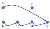
Figure 2: Semi-supervised learning example DAG for $\sigma_{\text{train}}=\{(u,v),(v,w),(w,x),(y,w)$: $\mathcal{NR}_{H_{s}}=\{v,w,x\}$ and $\mathcal{R}_{H_{s}}=\{u,y,z\}$.

Algorithm 1 summarizes our semi-supervised algorithm. The algorithm will become unsupervised when there is no $\sigma_{\text{train}}$ and step-5 is removed.

V Temporal Ordered Clustering for Duplication-Divergence Model

V-A Duplication-divergence model (DD-model)

We consider Solé et al. definition of the DD-model [20]. It proceeds as follows. Given an undirected, simple seed graph $G_{n_{0}}$ on $n_{0}$ nodes and target number of nodes $n$, the graph $G_{k+1}$ with $k+1$ nodes evolves from the $G_{k}$ as follows: first, a new vertex $v$ is added to $G_{k}$. Then the following steps are carried out:

• Duplication: Select a node $u$ from $G_{k}$ uniformly at random. The node $v$ then makes connections to $\mathcal{N}(u)$, the neighbor set of $u$.

• Divergence: Each of the newly made connections from $v$ to $\mathcal{N}(u)$ are deleted with probability $1-p$. Furthermore, for all the nodes in $G_{k}$ to which $v$ is not connected, create an edge from it to $v$ independently with probability $\frac{r}{k}$.

The above process is repeated until the number of nodes in the graph is equal to $n$. We denote the graph $G_{n}$ generated from the DD-model with parameters $p$ and $r$, starting from seed graph $G_{n_{0}}$, by $G_{n}\sim\texttt{DD-model}(n,p,r,G_{n_{0}})$.

The posterior probability $w(\delta(H_{s},z_{s}),H_{s})$, which is defined in (5) and used in Theorem 1 and high-prob-sampling, can be calculated for the DD-model as follows. For a node $z_{s}\in\mathcal{R}_{H_{s}}$, we say a node $u$ is its parent if $u$ can be selected from the graph $\delta(H_{s},z_{s})$ for the duplication step when $z_{s}$ is added into $\delta(H_{s},z_{s})$. The probability of having the node $u$ as the parent of $z_{s}\in\mathcal{R}_{H_{s}}$ in the DD-model is

$$w (\delta(H_{s},z_{s}),u,H_{s})$$

$$=\frac{1}{s-1}p^{|\mathcal{N}(z_{s})\cap\mathcal{N}(u)|}(1-p)^{|\mathcal{N}(u)\backslash\mathcal{N}(z_{s})|}$$

$$\quad\left(\frac{r}{s-1}\right)^{|\mathcal{N}(z_{s})\backslash\mathcal{N}(u)|}\left(1-\frac{r}{s-1}\right)^{(s-1)-|\mathcal{N}(z_{s})\cup\mathcal{N}(u)|}$$ (14)

The above expression can be inferred directly from the definition of the DD-model as follows. We first pick $u$ as a parent node of $z_{s}$ with probability $\frac{1}{s-1}$. Then to calculate the probabilities of edge addition events retrospectively, we observe that edges from $z_{s}$ to the nodes in the $\mathcal{N}(z_{s})\cap\mathcal{N}(u)$ stayed with probability $p$, but edges to $\mathcal{N}(u)\backslash\mathcal{N}(z_{s})$ were dismissed with probability $1-p$. We also have to take into account the edges between $z_{s}$ and vertices outside of $\mathcal{N}(u)$ – each were chosen independently with probability $\frac{r}{s-1}$ and they are exactly the edges from $z_{s}$ to $\mathcal{N}(z_{s})\backslash\mathcal{N}(u)$.

Now $w(\delta(H_{s},z_{s}),H_{s})=\sum_{u\in\mathcal{P}_{H_{s}}(z_{s})}w(\delta(H_{s},z_{s}),u,H_{s})$, where $\mathcal{P}_{H_{s}}(z_{s})$ represents possible parents of $z_{s}$ in $H_{s}$.

Since all permutations have positive probability in this version of the model, we have $\mathcal{R}_{H_{s}}=V(H_{s})$ and $\Gamma(H_{s})=s!$.

V-B Greedy algorithms for clustering

To form a comparison with algorithms proposed in Section IV, we propose the following greedy unsupervised algorithms for the DD-model.

sort-by-degree. The nodes are sorted by the degree and arranged into clusters $\{C_{i}\}_{i\geq 1}$. Cluster $C_{1}$ contains nodes with the largest degree.

peel-by-degree. The nodes with the lowest degree are first collected and put in the highest cluster. Then they are removed from the graph, and the nodes with the lowest degree in the remaining graph are found and the process repeats.

sort-by-neighborhood. This algorithm will output a partial order with all ordered pairs $(u\prec v)$ such that $\mathcal{N}(u)$ contains $\mathcal{N}(v)$. This condition holds when $r=0$. When $r>0$, we consider $|\mathcal{N}(v)\backslash N(u)|\leq r$ as $r$ is the average number of extra connections a node makes apart from duplication process. In most real-world data, we estimate $r$ as smaller than $1$, and hence the original check is sufficient.

peel-by-neighborhood. Here, we find the set $\{u:\nexists\,v|\mathcal{N}(v)\backslash\mathcal{N}(u)|\leq r\}$ (as mentioned before, it is sufficient to check $\mathcal{N}(v)\subset\mathcal{N}(u)$ in many practical cases) and mark it as the youngest cluster. These nodes are removed from the graph, and the process is repeated until it hits $G_{n_{0}}$. This algorithm makes use of the DAG of the neighborhood relationship and includes isolated nodes into the bins.

V-C Comparison with other graph models

The node arrival order recovery problem in the DD-model is different from that in other graph models like Erdős-Renyi graphs and preferential attachment graphs.

First, for a fixed graph $G_{n}$ on $n$ vertices, let us consider a set of graphs $\text{Adm}(G_{n})=\{\sigma(G_{n})\colon\sigma\in\Gamma(G_{n})\}$. It is obvious that for the Erdős-Renyi model, any graph in $\text{Adm}(G_{n})$ is generated equally likely with a given seed graph $G_{n_{0}}$. Such property was also proved for the preferential attachment model in [2]. However, this does not hold for DD-model graphs as shown in the following example.

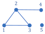
Figure 3: Example of asymmetric graph

For the graph $G_{n}^{(1)}$ presented in Figure 3, let $G_{n_{0}}$ consists of vertices $1$, $2$, $3$, and let the parameters of the DD-model be $p=0.2$ and $r=0$. The $\mathbb{P}[\mathcal{G}_{n}=G_{n}^{(1}]$ can be calculated iteratively using (14) as $0.068$. Now, consider the permutation

$$\sigma=\begin{pmatrix}1&2&3&4&5\\ 1&2&3&5&4\end{pmatrix}.$$

Then $\sigma\in\Gamma(G_{n}^{1})$. Let $G_{n}^{(2)}=\sigma(G_{n}^{(1)})$. The $\mathbb{P}[\mathcal{G}_{n}=G_{n}^{(2}]$ is $0.051$, and conditioned on the same structure probabilities of $G_{n}^{(1)}$ and $G_{n}^{(2)}$ are $0.5744$ and $0.4256$ respectively.

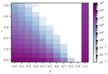
Figure 4: $\mathbb{E}\log|{\mathrm{Aut}}(G_{n})|$, $G_{n}\sim\texttt{DD-model}(2000,p,r,K_{20})$, where $|{\mathrm{Aut}}(G_{n})|$ is the number of automorphisms in graph $G_{n}$.

Second, it is well known that both the Erdős-Renyi graphs and preferential attachment graphs are asymmetric with high probability [6, 2]. On the other hand, the graphs generated from the DD-model for a certain range of parameters show a significant amount of symmetry, as shown in Fig. 4. This is in accordance with many real-world networks (see Table III for examples).

Last, the behavior of the degree at time $t$ of the node arrived at an earlier time $s$ (denoted by ${\text{deg}}_{t}(s)$) is different for all three models. For Erdős-Renyi graph with edge probability $p$, it is known that $\mathbb{E}[{\text{deg}}_{t}(s)]=p(t-1)$. For the preferential attachment graphs, $\mathbb{E}[{\text{deg}}_{t}(s)]=\Theta\left(\sqrt{t/s}\right)$ ([21], Theorem 8.2). However, for the DD-model, $\mathbb{E}[{\text{deg}}_{t}(s)]=\Theta\left(\left(t/s\right)^{p}s^{2p-1}\right)$ for any $t\geq s$ [7]. Note that when $s=O(1)$ – the case of very old nodes – the average degree is of order $t^{p}$. For $s=t$, we have $\mathbb{E}[{\text{deg}}_{t}(t)]=O(t^{2p-1})$ which is growing only for $p>1/2$. For example, when $p=1$ degrees of all the nodes on average are of order $O(t)$. Thus oldest nodes in the graph need not have large average degrees as the graph evolves, and algorithms based on such a heuristic are not applicable for the DD-model. Moreover, Frieze et al. [8] has shown that ${\text{deg}}_{t}(s)$ is concentrated around the mean for $s=O(1)$ in the sense that for any $A>1$ we observe polynomial tail:

$$\Pr [\text{deg}_{t}(s)<C\,\mathbb{E}[\text{deg}_{t}(s)\log^{-k}{t}]$$

$$=\Pr[\text{deg}_{t}(s)>C\,\mathbb{E}[\text{deg}_{t}(s)\log^{k}{t}]=O(t^{-A}),$$

for certain fixed constant $k$ and a constant $C$ dependent on $A$. However, this is not the case for the last vertices, since they are copied from already existing nodes in the network, which would explain the ineffectiveness of greedy degree-based heuristics for $p\leq 1/2$.

VI Experiments

In this section, we evaluate our methods on synthetic and real-world data sets. We made publicly available all the code and data of this project at https://github.com/krzysztof-turowski/duplication-divergence.

We present the following results in the coming sections.

• Synthetic networks:

  • How well the LP-partial-order performs in comparison with the LP-clusters? (Figures 5 and 6)

  • Fixing the LP-partial-order, how is the convergence of $p_{u,v}$’s that are estimated via sequential importance sampling schemes local-unif-sampling and high-prob-sampling as to the exact $p_{u,v}$, in terms of resulting precision? (Figure 7)

  • Fixing LP-partial-order for the LP formulation and local-unif-sampling for the importance sampling strategy, we study the performance of unsupervised algorithms in comparison with greedy strategies specific to the DD-model. (Figure 8)

  • For the semi-supervised algorithms, we show results (precision and density) for various parameter configurations and study their influence on the performance. (Tables I and II)

• Real-world networks: For the semi-supervised algorithms, how the precision improves with a small change in the training size, and how does the results compare against greedy algorithms of the DD-model? (Figure 9 and Table IV)

Maximum likelihood estimation

For deriving total order, a natural solution will be the maximum likelihood estimator (MLE).

$$\operatorname*{arg\,max}_{\sigma\in S_{n}}\mathbb{P}[\mathcal{G}_{n}={{{\pi}}}^{-1}(H_{n})|{{{\pi}}}^{-1}=\sigma]$$

But we do not consider MLE explicitly here because it is known that many networks exhibit large number of symmetries (see Table III for some examples), and thus there will be large number of total orders that achieve the MLE criterion with low value of precision. In fact, our optimal formulation in Section III already captures the MLE solutions and outputs them if they have high precision. Moreover for general graph models, the MLE computation would require checking all $\sigma\in S_{n}$ which incurs $\Theta(n!)$ computational complexity.

VI-A Synthetic networks

In the following results on synthetic networks, $\sigma_{\text{tries}}$ denote the number of Markov chain sample paths (for sequential importance sampling) used for estimating $p_{u,v}$ for all $u,v\in V(H_{n})$. All the studies are performed on multiple graph realizations from the DD-model with specified parameters, and the results are averaged over them. When we make a comparison based on LP formulation, we plot precision ($\theta$) vs minimum density $\varepsilon$ ($\delta\geq\varepsilon$) in accordance with the formulations in Sections III-A and III-B.

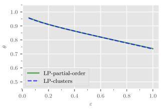
Figure 5: Comparison between LP-clusters and LP-partial-order formulation: $G_{n}\sim\texttt{DD-model}(n=30,p=0.6,r=1.0,G_{n_{0}}=K_{10})$ and $\sigma_{\text{tries}}=100,000$. Results are averaged over $100$ graph generations. Sampling method: local-unif-sampling.

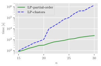
Figure 6: Time plot for LP-partial-order vs. LP-clusters. All the experiments were performed on 48-CPU cluster, with Intel(R) Xeon(R) CPU E7-8857 v2 @ 3.00GHz and 256GB RAM.

In Figure 5, we compare the performance of the linear programming approximations LP-cluster (Section III-A) and LP-partial-order (Section III-B). Since clustering output from the LP-cluster scheme induces a partial order, we use the same measures of precision and density that are defined for partial order for comparing performances of LP-cluster and LP-partial-order schemes. Our experiments confirm that for the same graph, with the same set of $\{p_{u,v},\forall u,v\in V(H_{n})\}$, the performance of them are nearly identical. However, Figure 6 shows that the difference between the running time of both the formulations is huge – the LP-clusters which finds clusters becomes barely feasible, whereas LP-partial-order which outputs partial order runs in a reasonable time.

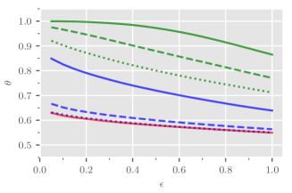
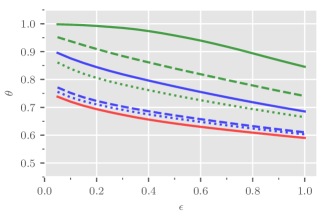
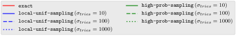
Figure 7: Results on synthetic networks with exact curve: $G_{n}\sim\texttt{DD-model}(13,p,1.0,G_{n_{0}})$ for $p=0.3$ (left) and $0.6$ (right), averaged over $100$ graphs. $G_{n_{0}}$ is generated from Erdős-Renyi graph with $n_{0}=4$ and $p_{0}=0.6$.

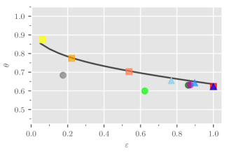
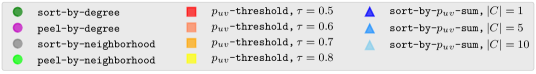
Figure 8: Results on synthetic networks with greedy and unsupervised learning $p_{u,v}$-based algorithms: $G_{n}\sim\texttt{DD-model}(50,p,1.0,G_{n_{0}})$ for $p=0.3$ (left) and $0.6$ (right), averaged over $100$ graphs. $p_{u,v}$-based algorithms use $\sigma_{\text{tries}}=100,\!000$. $G_{n_{0}}$ is generated from Erdős-Renyi model with $n_{0}=10$ and $p_{0}=0.6$. The theoretical curve is estimated via local-unif-sampling.

Figure 7 examines the precision of LP-partial-order obtained with approximated $\{p_{u,v},\forall u,v\in V(H_{n})\}$ via sequential importance strategies (local-unif-sampling and high-prob-sampling) and that obtained with the $\{p_{u,v},\forall u,v\in V(H_{n})\}$ that is calculated exactly by considering all the possible $n!$ orderings. We consider a small size ($n=13$) example here since it becomes infeasible to compute the exact curve for larger values of $n$. We observe that the convergence of the estimated curve is highly dependent on the method of estimation: local-unif-sampling method requires only $100$ samples, but high-prob-sampling is still visibly far away from LP optimal curve even for $1000$ samples. Thus, along with the computational reasons stated in Section IV, we use local-unif-sampling in the subsequent experiments.

In Figure 8, we compare results of the unsupervised algorithms with the estimated optimal curve via local-unif-sampling. It turns out that greedy algorithms (sort-by-degree, sort-by-neighborhood, peel-by-degree and peel-by-neighborhood) perform reasonably well for small $p$, but their performance deteriorates for higher values of $p$. On the other hand, $p_{u,v}$-based algorithms (sort-by-$p_{u,v}$-sum and $p_{u,v}$-threshold) offer consistent, close to the theoretical bound, behavior different values of $p$ (figure shows only two $p$s due to space limitations). Moreover, the bin size $|C|$ in sort-by-$p_{u,v}$-sum and threshold $\tau$ in $p_{u,v}$-threshold algorithm offer a trade-off between higher precision and higher density. The larger the bin size or the higher the threshold, we observe a decrease in density, but increase in precision as we stay close to the theoretical curve.

Table I contains the results of semi-supervised learning extensions of the $p_{u,v}$-based algorithms. A small increase in the percentage of the training set $\alpha$ yields a large increases in precision for all sets of parameters. Moreover, for larger bin size in sort-by-$p_{u,v}$-sum algorithm we observe mainly only an increase in precision with $\alpha$, but for $p_{u,v}$-threshold algorithm both $\delta$ and $\theta$ grow visibly with $\alpha$, especially for large $\tau$. In turn, when we fix $\alpha$ and increase the bin size in sort-by-$p_{u,v}$-sum algorithm, precision remains almost same, but density decreases significantly. And if we do the analogous procedure for $p_{u,v}$-threshold algorithm (fix $\alpha$ and increase threshold), then precision grows, but in expense of a visible fall of density. All the above conclusions are summarized in Table II.

		$p=0.3$		$p=0.6$
Algorithm	$\alpha$	$\delta$	$\theta$	$\delta$	$\theta$
sort-by-$p_{u,v}$-sum, $|C|=1$	$0.001$	$1.0$	$0.598$	$1.0$	$0.613$
sort-by-$p_{u,v}$-sum, $|C|=1$	$0.01$	$1.0$	$0.643$	$1.0$	$0.650$
sort-by-$p_{u,v}$-sum, $|C|=1$	$0.1$	$1.0$	$0.836$	$1.0$	$0.832$
sort-by-$p_{u,v}$-sum, $|C|=10$	$0.001$	$0.769$	$0.605$	$0.769$	$0.626$
sort-by-$p_{u,v}$-sum, $|C|=10$	$0.01$	$0.768$	$0.661$	$0.767$	$0.660$
sort-by-$p_{u,v}$-sum, $|C|=10$	$0.1$	$0.758$	$0.864$	$0.759$	$0.859$
$p_{u,v}$-threshold, $\tau=0.5$	$0.001$	$1.0$	$0.604$	$1.0$	$0.617$
$p_{u,v}$-threshold, $\tau=0.5$	$0.01$	$1.0$	$0.637$	$1.0$	$0.649$
$p_{u,v}$-threshold, $\tau=0.5$	$0.1$	$1.0$	$0.829$	$1.0$	$0.823$
$p_{u,v}$-threshold, $\tau=0.9$	$0.001$	$0.010$	$0.906$	$0.028$	$0.871$
$p_{u,v}$-threshold, $\tau=0.9$	$0.01$	$0.020$	$0.951$	$0.090$	$0.907$
$p_{u,v}$-threshold, $\tau=0.9$	$0.1$	$0.521$	$0.966$	$0.559$	$0.960$

TABLE I: Results on synthetic networks with semi-supervised learning $p_{u,v}$-based algorithms: $G_{n}\sim\texttt{DD-model}(50,p,1.0,G_{n_{0}})$, averaged over $100$ graphs. $p_{u,v}$-based algorithms use $\sigma_{\text{tries}}=100,000$. $G_{n_{0}}$ is Erdős-Renyi graph with $n_{0}=10$ and $p_{0}=0.6$.

Algorithm	Fixed	Free	Free	Free
sort-by-$p_{u,v}$-sum	$\alpha$	$|C|\nearrow$	$\delta\searrow$	$\theta\approx$
sort-by-$p_{u,v}$-sum	$|C|$	$\alpha\nearrow$	$\delta\approx$	$\theta\nearrow$
$p_{u,v}$-threshold	$\alpha$	$\tau\nearrow$	$\delta\searrow$	$\theta\nearrow$
$p_{u,v}$-threshold	$\tau$	$\alpha\nearrow$	$\delta\nearrow$	$\theta\nearrow$

TABLE II: Conclusions from synthetic data: how the metrics behave by fixing one of the parameters and keeping other free. The symbol $\approx$ indicates the changes are not significant.

VI-B Real-world networks

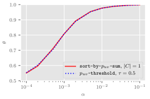
(a) ArXiv network

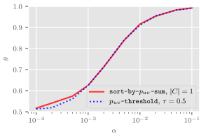
(b) Simple English Wikipedia network

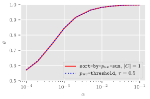
(c) CollegeMsg network

Figure 9: Real-world networks: results of semi-supervised learning

We consider the following three real-world networks which have the ground truth of node and edge age arrival order available. The directed networks are treated as undirected in our studies. All the datasets are taken from SNAP repository [22].

• The ArXiv network: It is a directed network with $7,\!464$ nodes and $116,\!268$ edges. Here the nodes are the publications in arXiv online repository of theoretical high energy physics, and the edges are formed when a publication cite another. In this network, many nodes share the same arrival time and date, and hence the true arrival order of nodes is available only in bins of count $1,\!457$.

• The Simple English Wikipedia dynamic network: A directed network with $10,\!000$ nodes and $169,\!894$ edges. Nodes represent articles and an edge indicates that a hyperlink was added. It shows the evolution of hyperlinks between articles of the Simple English Wikipedia.

• CollegeMsg network: In this dataset of private message sent on an online social platform at University of California, Irvine, nodes represent users and an edge from $u$ to $v$ indicates user $u$ sent a private message to user $v$ at time $t$. Number of nodes is $1,\!899$ and number of edges is $59,\!835$.

Table III shows estimated parameters of the duplication-divergence model for the above networks using the fitting technique in [23].

Network ($G_{\text{obs}}$)	$\log|{\mathrm{Aut}}(G_{\text{obs}})|$	$\widehat{p}$	$\widehat{r}$
ArXiv	$12.59$	$0.72$	$1.0$
Wikipedia	$1018.94$	$0.66$	$0.5$
CollegeMsg	$231.54$	$0.65$	$0.45$

TABLE III: Parameters of the duplication-divergence model estimated for the real-world networks considered in this paper.

Figure 9 show the result of semi-supervised learning. Here $\alpha$ represents the proportion of all pairs that is considered as training set, i.e., size of the training set is $\alpha\binom{n}{2}$. We randomly pick $\alpha\binom{n}{2}$ pairs and the results presented are average over $100$ different such random sets. We observe that a small increase in $\alpha$ leads to a huge change in the precision. This also happens in synthetic data and is caused by the large structural dependency within networks, unlike in classical machine learning where data is often assumed to be independent. This helps us to get a near-perfect clustering (precision close to $1$) with only $1\%$ of the labeled nodes.

Finally, the semi-supervised approach helps to obtain a significant improvement over greedy algorithms. As it is shown in Table IV, greedy algorithms found orderings with precision ranging from $0.47$ to $0.63$ for significant values of the density (it’s easy to achieve a precision of $0.78$ like CollegeMsg data set when the density of pairs outputted is as low $0.01$) – which is not much better than random guess.

	ArXiv		Wikipedia		CollegeMsg
Greedy algorithm	$\delta$	$\theta$	$\delta$	$\theta$	$\delta$	$\theta$
sort-by-degree	$0.98$	$0.47$	$0.96$	$0.59$	$0.92$	$0.63$
peel-by-degree	$0.98$	$0.46$	$0.96$	$0.59$	$0.92$	$0.63$
sort-by-neighborhood	$0.0001$	$0.51$	$0.03$	$0.60$	$0.01$	$0.78$
peel-by-neighborhood	$0.13$	$0.50$	$0.80$	$0.593$	$0.75$	$0.61$

TABLE IV: Real-world networks: results of greedy algorithms.

VII Discussion and future work

In this article we presented a framework for clustering of nodes in dynamic networks based on latent temporal information. We provided a way to find an upper bound on the optimum clustering quality, and proposed several algorithms that perform well and capable of including some external information about the precedence of vertices in their arrival to the network.

Further work in our proposed framework can go in several directions. For example, one can explore various ways to speed up the algorithms presented in this work. This can be accomplished by finding a good importance sampling distribution, which will lead to a faster convergence of estimates of $p_{u,v}$ (probability that node $u$ is arrived earlier than node $v$), for all the nodes $u$ and $v$ in the network, to the true values. From a theoretical perspective, there remains an interesting question of finding bounds on the convergence speed of estimates of ${p}_{u,v}$ with various importance sampling distributions. One can also look into clever bookkeeping techniques which will result in reducing the computation time of a single path in our sequential importance sampling algorithm. Another direction is the application of the proposed framework and solution to other types of random network models that not only involve only the addition of vertices and edges, but also deletion of them.

Jithin K. Sreedharan is a Postdoctoral Research Associate at the NSF Center for Science of Information and Dept. of Computer Science in Purdue University. He received his Ph.D. in computer science from INRIA, France, in 2017 with a fellowship from INRIA-Bell Labs joint lab. Before that, he finished M.S. from Indian Institute of Science (IISc), Bangalore, in 2013, and received the best thesis award. His current works focus on data mining algorithms for large networks with probabilistic guarantees, statistical modeling and inference on networks, and distributed techniques for analyzing big matrices.

Krzysztof Turowski is currently assistant professor at the Theoretical Computer Science Department at the Jagiellonian University, Krakow, Poland. He received his MS and PhD degrees from Gdansk University of Technology, Poland in 2011 and 2015, respectively, both in computer science. From 2010 to 2016 he was employed at the Department of Algorithms and System Modelling at Gdansk University of Technology and from 2016 to 2018 he worked at Google as a software developer for Google Compute Engine. From 2018 to 2019 he was a Postdoctoral Research Scholar in the NSF Center for Science of Information at Purdue University. His research interests include graph theory (especially various models of graph coloring), analysis of algorithms and information theory.

Wojciech Szpankowski is Saul Rosen Distinguished Professor of Computer Science at Purdue University where he teaches and conducts research in analysis of algorithms, information theory, analytic combinatorics, data science, random structures, and stability problems of distributed systems. He held several Visiting Professor/Scholar positions, including McGill University, INRIA, France, Stanford, Hewlett-Packard Labs, Universite de Versailles, University of Canterbury, New Zealand, Ecole Polytechnique, France, the Newton Institute, Cambridge, UK, ETH, Zurich, and Gdansk University of Technology, Poland. He is a Fellow of IEEE, and the Erskine Fellow. In 2010 he received the Humboldt Research Award and in 2015 the Inaugural Arden L. Bement Jr. Award. He is also the recipient of 2020 Flajolet Lecture Prize. He published two books: “Average Case Analysis of Algorithms on Sequences”, John Wiley & Sons, 2001, and “Analytic Pattern Matching: From DNA to Twitter”, Cambridge, 2015. In 2008 he launched the interdisciplinary Institute for Science of Information, and in 2010 he became the Director of the newly established NSF Science and Technology Center for Science of Information.

References

- [1] S. E. Schaeffer, “Graph clustering,” Computer Science Review, vol. 1, no. 1, pp. 27–64, 2007.
- [2] T. Łuczak, A. Magner, and W. Szpankowski, “Asymmetry and structural information in preferential attachment graphs,” Random Structures and Algorithms, pp. 1–23, 2019.
- [3] K. Turowski, A. Magner, and W. Szpankowski, “Compression of Dynamic Graphs Generated by a Duplication Model,” in 56th Annual Allerton Conference on Communication, Control, and Computing, Allerton 2018, Monticello, IL, USA, October 2-5, 2018, 2018, pp. 1089–1096.
- [4] M. Srivastava, O. Simakov, J. Chapman, B. Fahey, M. E. Gauthier, T. Mitros, G. S. Richards, C. Conaco, M. Dacre, U. Hellsten et al., “The amphimedon queenslandica genome and the evolution of animal complexity,” Nature, vol. 466, no. 7307, p. 720, 2010.
- [5] J. K. Sreedharan, A. Magner, A. Grama, and W. Szpankowski, “Inferring temporal information from a snapshot of a dynamic network,” Scientific Reports, vol. 9, no. 1, p. 3057, 2019.
- [6] J. H. Kim, B. Sudakov, and V. Vu, “On the asymmetry of random regular graphs and random graphs,” Random Structures & Algorithms, vol. 21, no. 3-4, pp. 216–224, 2002.
- [7] K. Turowski and W. Szpankowski, “Towards degree distribution of duplication graph models,” 2019, https://www.cs.purdue.edu/homes/spa/papers/random19.pdf.
- [8] A. Frieze, K. Turowski, and W. Szpankowski, “Degree distribution for duplication-divergence graphs: Large deviations,” 2020, to appear in Proceedings of WG 2020: 46th International Workshop on Graph-Theoretic Concepts in Computer Science.
- [9] A. Loukas and P. Vandergheynst, “Spectrally approximating large graphs with smaller graphs,” in International Conference on Machine Learning, Stockholm, Sweden, 2018, pp. 3243–3252.
- [10] F. Liu, D. Choi, L. Xie, and K. Roeder, “Global spectral clustering in dynamic networks,” Proceedings of the National Academy of Sciences, vol. 115, no. 5, pp. 927–932, 2018.
- [11] R. Görke, P. Maillard, C. Staudt, and D. Wagner, “Modularity-driven clustering of dynamic graphs,” in International Symposium on Experimental Algorithms. Berlin, Heidelberg: Springer, 2010, pp. 436–448.
- [12] D. Greene, D. Doyle, and P. Cunningham, “Tracking the evolution of communities in dynamic social networks,” in 2010 International Conference on Advances in Social Networks Analysis and Mining. Washington, DC, USA: IEEE, 2010, pp. 176–183.
- [13] E. Bair, “Semi-supervised clustering methods,” Wiley Interdisciplinary Reviews: Computational Statistics, vol. 5, no. 5, pp. 349–361, 2013.
- [14] S. Basu, A. Banerjee, and R. Mooney, “Semi-supervised clustering by seeding,” in International Conference on Machine Learning. San Francisco, CA, USA: Morgan Kaufmann Publishers Inc., 2002, pp. 27–34.
- [15] B. Kulis, S. Basu, I. Dhillon, and R. Mooney, “Semi-supervised graph clustering: a kernel approach,” Machine Learning, vol. 74, no. 1, pp. 1–22, 2009.
- [16] S. Li, K. P. Choi, T. Wu, and L. Zhang, “Maximum likelihood inference of the evolutionary history of a ppi network from the duplication history of its proteins,” IEEE/ACM Transactions on Computational Biology and Bioinformatics (TCBB), vol. 10, no. 6, pp. 1412–1421, 2013.
- [17] S. Navlakha and C. Kingsford, “Network archaeology: uncovering ancient networks from present-day interactions,” PLoS Computational Biology, vol. 7, no. 4, p. e1001119, 2011.
- [18] K. Turowski, J. K. Sreedharan, and W. Szpankowski, “Temporal ordered clustering in dynamic networks,” 2020, to appear in Proceedings of IEEE International Symposium on Information Theory.
- [19] S. Boyd and L. Vandenberghe, Convex Optimization. Cambridge University Press, 2004.
- [20] R. Pastor-Satorras, E. Smith, and R. V. Solé, “Evolving protein interaction networks through gene duplication,” Journal of Theoretical Biology, vol. 222, no. 2, pp. 199–210, 2003.
- [21] R. Van Der Hofstad, Random graphs and complex networks. Cambridge: Cambridge University Press, 2016, vol. 1.
- [22] J. Leskovec and A. Krevl, “SNAP Datasets: Stanford large network dataset collection,” http://snap.stanford.edu/data, Jun. 2014.
- [23] J. K. Sreedharan, K. Turowski, and W. Szpankowski, “Revisiting parameter estimation in biological networks: Influence of symmetries,” IEEE/ACM Transactions on Computational Biology and Bioinformatics, 2020, http://doi.org/10.1109/TCBB.2020.2980260.