Anti-Zeno quantum advantage in fast-driven heat machines

Abstract

Developing quantum machines which can outperform their classical counterparts, thereby achieving quantum supremacy or quantum advantage, is a major aim of the current research on quantum thermodynamics and quantum technologies. Here we show that a fast-modulated cyclic quantum heat machine operating in the non-Markovian regime can lead to significant heat-current and power boosts induced by the anti-Zeno effect. Such boosts signify a quantum advantage over almost all heat-machines proposed thus far that operate in the conventional Markovian regime, where the quantumness of the system-bath interaction plays no role. The present effect owes its origin to the time-energy uncertainty relation in quantum mechanics, which may result in enhanced system-bath energy exchange for modulation periods shorter than the bath correlation-time.

Introduction

The non-equilibrium thermodynamic description of heat machines consisting of quantum systems coupled to heat baths is almost exclusively based on the Markovian approximation breuer02 ; rivas12open . This approximation allows for monotonic convergence of the system-state to thermal equilibrium with its environment (bath) and yields a universal bound on entropy change (production) in the system spohn78entropy . Yet, the Markovian approximation is not required for the derivation of the Carnot bound on the efficiency of a cyclic two-bath heat engine (HE): this bound follows from the second law of thermodynamics, under the condition of zero entropy change over a cycle by the working fluid (WF), in both classical and quantum scenarios. In general, the question whether non-Markovianity is an asset remains open, although several works have ventured into the non-Markovian domain mukherjee15 ; uzdin16quantum ; pezzutto18an ; thomas18thermodynamics ; nahar18preparations ; abiuso19non . By contrast, it has been suggested that quantum resources, such as a bath consisting of coherently superposed atoms scully03extracting , or a squeezed thermal bath rossnage14nanoscale ; klaers17squeezed ; niedenzu18quantum , may raise the efficiency bound of the machine. The mechanisms that can cause such a raise include either a conversion of atomic coherence and entanglement in the bath into WF heatup scully03extracting ; abah14efficiency ; dag18temperature , or the ability of a squeezed bath to exchange ergotropy rossnage14nanoscale ; niedenzu16on ; klaers17squeezed ; niedenzu18quantum (alias non-passivity or work-capacity pusz78 ; lenard78 ; klimovsky15 ) with the WF, which is incompatible with a standard HE. However, neither of these mechanisms is exclusively quantum; both may have classical counterparts ghosh18are . Likewise, quantum coherent or squeezed driving of the system acting as a WF or a piston ghosh17catalysis may boost the power output of the machine depending on the ergotropy of the system state, but not on its non-classicality niedenzu18quantum .

Finding quantum advantages in machine performance relative to their classical counterparts has been one of the major aims of research in the field of quantum technology in general kurizki15quantum ; harrow17quantum ; boixo18characterizing , and particularly in thermodynamics of quantum systems ghosh2018thermodynamic . Overall, the foregoing research leads to the conclusion that conventional thermodynamic description of cyclic machines based on a (two-level, multilevel or harmonic oscillator) quantum system in arbitrary two-bath settings may not be the arena for a distinct quantum advantage in machine performance ghosh18are . An exception should be made for multiple identical machines that exhibit collective, quantum-entangled features niedenzu18cooperative ; campo16quantum ).

Here we show that quantum advantage is in fact achievable in a quantum heat machine (QHM), whether a heat engine or a refrigerator, whose energy-level gap is modulated faster than what is allowed by the Markov approximation. To this end, we invoke methods of quantum system-control via frequent coherent (e.g. phase-flipping or level-modulating) operations kofman01universal ; kofman04unified as well as their incoherent counterparts (e.g. projective measurements or noise-induced dephasing) kofman00acceleration ; erez08 ; gordon09cooling ; gordon10equilibration ; alvarez10zeno . Such control has previously been shown, both theoreticallykofman00acceleration ; gordon07universal ; erez08 ; clausen10bath and experimentally alvarez10zeno ; almog11direct , to yield non-Markovian dynamics that conforms to one of two universal paradigms: i) quantum Zeno dynamics (QZD) whereby the bath effects on the system are drastically suppressed or slowed down; ii) anti-Zeno dynamics (AZD) that implies the opposite, i.e., enhancement or speedup of the system-bath energy exchange kofman00acceleration ; erez08 ; rao11from . It has been previously shown that QZD leads to the heating of both the system and the bath at the expense of the system-bath correlation energy klimovsky13work , whereas AZD may lead to alternating cooling or heating of the system at the expense of the bath or vice-versa kofman00acceleration ; erez08 . In our present analysis of cyclic heat machines based on quantum systems, we show that analogous effects can drastically modify the power output, without affecting their Carnot efficiency bound. AZD is shown to bring about a drastic power boost, thereby manifesting genuine quantum advantage, as it stems from the time-energy uncertainty relation of quantum mechanics.

Results

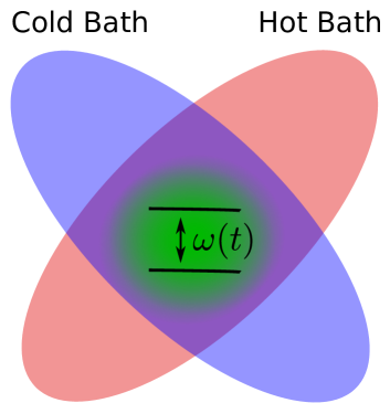
Figure 1: A two-level system thermal machine: Schematic setup showing a two-level system with periodically modulated level distance $\omega(t)$ as the working fluid (WF) in a thermal machine wherein the WF is simultaneously coupled to hot and cold baths with non-overlapping spectra. Possible realizations include a driven-atom WF coupled to filtered heat baths in a cavity or a driven impurity coupled to spectrally distinct phonon baths in a solid structure klimovsky13minimal ; ghosh18we .

Model. We consider a quantum system $\mathcal{S}$ that plays the role of a working fluid (WF) in a quantum thermal machine, wherein it is simultaneously coupled to cold and hot thermal baths. The system is periodically driven or perturbed with time period $\tau_{\rm S}=2\pi/\Delta_{\rm S}$ by the time-dependent Hamiltonian $\hat{H}_{\rm S}(t)$:

$$\hat{H}_{\rm S}(t+\tau_{\rm S})=\hat{H}_{\rm S}(t).$$ (1)

In order to have frictionless dynamics at all times, we choose $\hat{H}_{\rm S}(t)$ to be diagonal in the energy basis of $\mathcal{S}$, such that.

$$\left[\hat{H}_{\rm S}(t),\hat{H}_{\rm S}(t^{\prime})\right] = 0\leavevmode\nobreak\ \leavevmode\nobreak\ \leavevmode\nobreak\ \forall\leavevmode\nobreak\ t,t^{\prime}.$$ (2)

The system interacts simultaneously with the independent cold (c) and hot (h) baths via

$$\hat{H}_{\rm I}=\sum_{j={\rm c,h}}\hat{S}\otimes\hat{B}_{j},$$ (3)

where the bath operators $\hat{B}_{\rm c}$ and $\hat{B}_{\rm h}$ commute: $\left[\hat{B}_{\rm c},\hat{B}_{\rm h}\right]=0$, and $\hat{S}$ is a system operator. For example, for a two level system, $\hat{S}=\hat{\sigma}_{x}$, while $\hat{S}=\hat{X}$ for a harmonic oscillator, in standard notations. We do not invoke the rotating wave approximation in the system-bath interaction Hamiltonian Eq. (3). As in the minimal continuous quantum heat machine klimovsky13minimal , or its multilevel extensions mukherjee16speed , we require the two baths to have non-overlapping spectra, e.g., super-Ohmic spectra with distinct upper cut-off frequencies (see Fig. 1). This requirement allows $\mathcal{S}$ to effectively couple intermittently to one or the other bath during the modulation period $\tau_{\rm S}$, without changing the interaction Hamiltonian to either bath.

From Markovian to non-Markovian dynamics. In what follows we assume weak system-bath coupling, consistent with the Born (but not necessarily the Markov) approximation. Our goal is to examine the dynamics as we transit from Markovian to non-Markovian time scales, and the ensuing change of the QHM performance as the period duration $\tau_{\rm S}$ is decreased. To this end, we have adopted the methodology previously derived in Refs. kofman01universal ; kofman04unified ; shahmoon13 ; kosloff13quantum , to account for the periodicity of $\hat{H}_{\rm S}(t)$, by resorting to a Floquet expansion of the Liouville operator in the harmonics of $\Delta_{\rm S}=2\pi/\tau_{\rm S}$ szczygielski13 ; alicki14quantum ; klimovsky13minimal . As explained below, we focus on system-bath coupling durations $\tau_{\rm C}=n\tau_{\rm S}$ of the order of a few modulation periods, where $n>1$ denotes the number of periods. The time-scales of importance are the modulation time period $\tau_{\rm S}$, the system-bath coupling duration $\tau_{\rm C}$, the bath correlation-time $\tau_{\rm B}$ and the thermalization time $\tau_{\rm th}\sim\gamma_{0}^{-1}$, where $\gamma_{0}$ is the system-bath coupling strength. We consider $n\gg 1$ such that $\tau_{\rm C}\gg\tau_{\rm S},\leavevmode\nobreak\ \left(\omega+q\Delta_{\rm S}\right)^{-1}$, where $\omega$ denotes the transition frequencies of the system $\mathcal{S}$, and $q$ is an integer (see Methods “Floquet Analysis of the non-Markovian Master Equation”). This allows us to implement the secular approximation, thereby averaging over the fast-rotating terms in the dynamics. In the limit of slow modulation, i.e, $\tau_{\rm S}\gg\tau_{\rm B}$, we have $\tau_{\rm C}\gg\tau_{\rm B}$, which allows us to perform the Born, Markov and secular approximations, and eventually arrive at a time-independent Markovian master equation for $\tau_{\rm C}\gg\tau_{\rm S},\leavevmode\nobreak\ \omega^{-1},\leavevmode\nobreak\ \tau_{\rm B}$ (see Methods “Floquet Analysis of the non-Markovian Master Equation”).

On the other hand, in the regime of fast modulation $\tau_{\rm S}\ll\tau_{\rm B}$, the Markov approximation becomes inapplicable for coupling durations $\tau_{\rm C}=n\tau_{\rm S}\lesssim\tau_{\rm B}$. This gives rise to the fast-modulation form of the master equation (see Methods. “Floquet Analysis of the non-Markovian Master Equation” and “Non-Markovian dynamics of a driven two-level system in a dissipative bath”):

$$\dot{\rho}_{\rm S}(t) = \sum_{j={\rm h,c}}\mathcal{L}_{j}\left[\rho_{\rm S}(t)\right]$$

$$= \sum_{j,\omega}\tilde{\mathcal{I}}_{j}(\omega,t)\mathcal{D}_{j,\omega}\left[\rho_{\rm S}(t)\right]+\text{h.c.};$$

$$\tilde{\mathcal{I}}_{j}(\omega,t) \equiv \int_{-\infty}^{\infty}d\nu G_{j}(\nu)\Big{[}\frac{\sin\left[\left(\nu-\omega\right)t\right]}{\nu-\omega}$$ (4)

$$\pm i\left(\frac{\cos\left[\left(\nu-\omega\right)t\right]-1}{\nu-\omega}\right)\Big{]}$$

For simplicity, unless otherwise stated, we consider $\hbar=k_{\rm B}=1$. Here, for any modulation period $\tau_{\rm S}$, the generalized Liouville operators $\mathcal{L}_{j}$ of the two baths act additively on the reduced density matrix $\rho_{\rm S}(t)$ of $\mathcal{S}$, generated by the $\omega$-spectral components of the Lindblad dissipators $\mathcal{D}_{j,\omega}$ (see below) for the $j={\rm c,h}$ bath acting on $\rho_{\rm S}(t)$. For a two-level system, or an oscillator, $\mathcal{D}$ does not depend on $\omega$ breuer02 . For $\rho_{\rm S}(t)$ that is diagonal in the energy basis, which we consider below, the dynamics is dictated by the coefficients $\mathcal{I}_{j}(\omega,t)\equiv{\rm Re}\left[\tilde{\mathcal{I}}_{j}(\omega,t)\right]$ in Eq. (4), which express the convolution of the $j$-th bath spectral response function $G_{j}(\nu)$ that has spectral width $\sim\Gamma_{\rm B}\sim 1/\tau_{\rm B}$, with the sinc function, imposed by the time-energy uncertainty relation for finite times (see Methods “Non-Markovian dynamics of a driven two-level system in a dissipative bath”).

Our main contention is that overlap between the sinc function and $G_{j}(\nu)$ at $t\sim\tau_{\rm C}\lesssim\tau_{\rm B}$ may lead to the anti-Zeno effect, i.e., to remarkable enhancement in the convolution $\mathcal{I}_{j}(\omega,t)$, and, correspondingly, in the heat currents and power. One can stay in this regime of enhanced performance over many cycles, by running the QHM in the following two-stroke non-Markovian cycles:
i) Stroke 1: we run the QHM by keeping the WF (system) and the baths coupled over $n$ modulation periods, from time $t=0$ to $t=n\tau_{\rm S}=\tau_{\rm C}\lesssim\tau_{\rm B}$ ($n\gg 1$, $\tau_{\rm S}\ll\tau_{\rm B}$). The $n$ modulation periods of the WF are equivalent to $n$ cycles of continuous heat machines studied earlier, which have been shown to exploit spectral separation of the hot and cold baths for the extraction of work klimovsky13minimal ; alicki14quantum , or refrigeration klimovsky15 ; kolar12 , in the Markovian regime (see Eq. (8)). By contrast, in the non-Markovian domain a modulation period is not a cycle, since the time-dependent heat currents and the WF state are not necessarily reset to their initial values at the beginning of each modulation period (see below).
ii) Stroke 2: In order to reset the WF state and the heat currents to their initial ($t=0$) values in the non-Markovian regime, we have to add another stroke: At $t=n\tau_{\rm S}=\tau_{\rm C}$, we decouple the WF from the hot and cold baths. One needs to keep the WF and the thermal baths uncoupled (non-interacting) for a time-interval $\bar{t}\gtrsim\tau_{\rm B}$, so as to eliminate all the transient memory effects rao11from .
After this decoupling period, we recouple the WF to the hot and cold thermal baths and continue to drive the WF with the periodically modulated Hamiltonian Eq. (1). Thus the setup is initialized

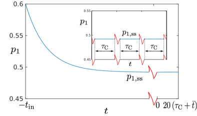
Figure 2: Time-evolution: Time-evolution of the $|1\rangle$-state probability $p_{1}(t)$ of a two-level system working fluid (WF). The WF is first connected to the hot and cold baths, whose quasi-Lorentzian spectral functions are given by Eq. (54), at a negative time $-t_{in}$ $(t_{in}\gg\tau_{\rm th})$, under the initial condition $p_{1}(t=-t_{\rm in})=0.6$, and reaches the steady-state value $p_{1,{\rm ss}}$ at $t+t_{\rm in}\gg\tau_{\rm th}$. The WF is decoupled from the hot and cold thermal baths at a time $-\bar{t}\lesssim-\tau_{\rm B}<0$ after reaching the steady-state, and then recoupled again to the two baths at time $t=0$, such that the WF is non-interacting with the hot and cold thermal baths for the time interval $-\bar{t}\leq t<0$, shown by the red break-line. The quantum heat machine is operated in the anti-Zeno dynamics (AZD) regime for $t\geq 0$, wherein it is decoupled from and recoupled to the thermal baths after every AZD cycle, for coupling time duration $\tau_{\rm C}=n\tau_{\rm S}$. The probability $p_{1}$ remains unchanged at the steady-state value, even after multiple AZD cycles. Inset: Same as the main plot, zoomed in for three consecutive AZD cycles. The WF is non-interacting with the thermal baths for time intervals $\bar{t}\gtrsim\tau_{\rm B}$ between two consecutive AZD cycles, shown by the red break lines. Here (see Eqs. (7) - (11)) $\lambda=0.2,\omega_{0}=20,\Delta_{\rm S}=10,n=10,\beta_{\rm h}=0.0005,\beta_{\rm c}=0.005$, and we consider quasi-Lorentzian bath spectral functions Eq. (54) with $\gamma_{0}=1,\Gamma_{\rm B}=0.2,\delta_{\rm h}=\delta_{\rm c}=1,\alpha=1.$

after time $\tau_{\rm C}+\bar{t}$, provided we choose $n$ to be such that $\rho_{\rm S}(\tau_{\rm C}+\bar{t})=\rho_{\rm S}(0)$, so as to close the steady-state cycle after $n$ modulation periods, with the WF returning to its state at start of the cycle (see Fig. 2 and Sec. “A minimal quantum thermal machine beyond Markovianity”). The QHM may then run indefinitely in the non-Markovian cyclic regime.

By contrast, in the limit of long WF-baths coupling duration $\tau_{\rm C}=n\tau_{\rm S}\gg\tau_{\rm B}$, the ${\rm sinc}$ functions take the form of delta functions, and therefore, as expected, the integral Eq. (4) reduces to the standard form obtained in the Markovian regime, given by

$$\mathcal{I}_{j}(\omega,t)=\pi G_{j}\left(\omega\right)>0\leavevmode\nobreak\ .$$ (5)

A minimal quantum thermal machine beyond Markovianity. Here we consider as the QHM a two-level system (TLS) WF with states $|0\rangle$ and $|1\rangle$, interacting with a hot and a cold thermal bath, described by the Hamiltonian

$$\hat{H}(t)=\hat{H}_{\rm S}(t)+\hat{\sigma}_{x}\otimes\left(\hat{B}_{\rm c}+\hat{B}_{\rm h}\right)+\hat{H}_{\rm B}.$$ (6)

The Pauli matrices $\hat{\sigma}_{j}$ ($j=x,y,z$) act on the TLS, the operator $\hat{B}_{\rm c}$ ($\hat{B}_{\rm h}$) acts on the cold (hot) bath, and $\hat{H}_{\rm B}$ denotes the bath Hamiltonian. The resonance frequency $\omega(t)$ of the TLS is sinusoidally modulated by the periodic-control Hamiltonian

$$\hat{H}_{\rm S}(t) = \frac{1}{2}\omega(t)\hat{\sigma}_{z};\leavevmode\nobreak\ \leavevmode\nobreak\ \leavevmode\nobreak\ \leavevmode\nobreak\ \sigma_{z}|1\rangle=|1\rangle,\leavevmode\nobreak\ \sigma_{z}|0\rangle=-|0\rangle$$

$$\omega(t) = \omega_{0}+\lambda\Delta_{\rm S}\sin\left(\Delta_{\rm S}t\right),$$ (7)

where the relative modulation amplitude is small: $0<\lambda\ll 1$. The periodic modulation Eq. (7) gives rise to Floquet sidebands (denoted by the index $q=0,\pm 1,\pm 2,\ldots$) with frequencies $\omega_{q}=\left(\omega_{0}+q\Delta_{\rm S}\right)$ and weights $P_{q}$, which diminish rapidly with increasing $|q|$ for small $\lambda$ (see Methods “Non-Markovian dynamics of a driven two-level system in a dissipative bath”) kofman04unified ; kosloff13quantum ; klimovsky13minimal .

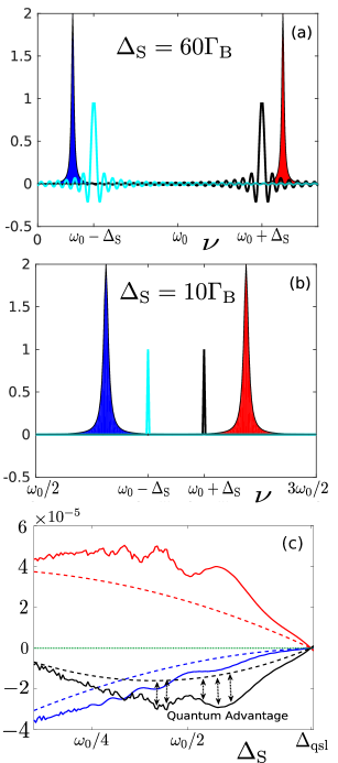
Figure 3: Quantum advantage with quasi-Lorentzian spectral functions: The quasi-Lorentzian spectral functions of the hot bath $G_{\rm h}(\nu)$ (red filled curve) and the cold bath $G_{\rm c}(\nu)$ (blue filled curve) (see Eq. (54)), and the sinc functions ${\rm sinc}\left[\left(\nu-\omega_{0}-\Delta_{\rm S}\right)t\right]$ (black solid curve) and ${\rm sinc}\left[\left(\nu-\omega_{0}+\Delta_{\rm S}\right)t\right]$ (cyan solid curve) for (a) fast modulation $\Delta_{\rm S}=60\Gamma_{\rm B}$ and (b) slow modulation $\Delta_{\rm S}=10\Gamma_{\rm B}$, at $t=10\tau_{\rm S}$. Fast (slow) modulation results in broadening (narrowing) of the sinc functions, thus leading to enhanced (reduced) overlap with the spectral functions. (c) Power $\overline{\dot{W}}$ (black lines) and heat currents $\overline{J_{\rm h}}$ (red lines) and $\overline{J_{\rm c}}$ (blue lines) averaged over $n=10$ modulation periods (solid lines) and the same obtained under the Markovian approximation for long cycles, i.e., large number of modulation periods ($n\to\infty$) (dashed lines), versus the modulation frequency $\Delta_{\rm S}$. Anti-Zeno dynamics for $\tau_{\rm C}\lesssim\tau_{\rm B}$ results in output power boost (shown by dotted double-arrowed lines) by up to more than a factor of $2$, signifying quantum advantage in the heat-engine regime. The green dotted line corresponds to zero power and currents. Here $\lambda=0.2,\omega_{0}=20,\gamma_{0}=1,\Gamma_{\rm B}=0.2,N=1,\delta=3,\epsilon=0.01,\alpha=1,\beta_{\rm h}=0.0005,\beta_{\rm c}=0.005$.

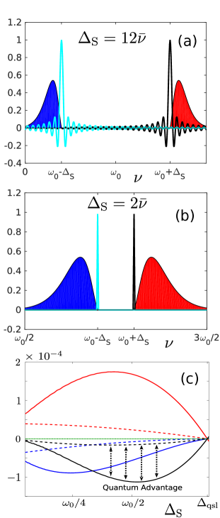
Figure 4: Quantum advantage with super-Ohmic spectral functions: Overlap of super-Ohmic spectral functions $G_{\rm h}(\nu)$ (red filled curve) and $G_{\rm c}(\nu)$ (blue filled curve) with cutoff frequency $\bar{\nu}$ (see Eq. (55)), with the modulation response functions ${\rm sinc}\left[\left(\nu-\omega_{0}-\Delta\right)t\right]$ (black solid curve) and ${\rm sinc}\left[\left(\nu-\omega_{0}+\Delta\right)t\right]$ (cyan solid curve) for (a) fast modulation, $\Delta_{\rm S}=12\bar{\nu}$, and (b) slow modulation $\Delta_{\rm S}=2\bar{\nu}$ at $t=10\tau_{\rm S}$. Fast (slow) modulation results in broad (narrow) sinc functions, and thus enhanced (reduced) overlap with the spectral functions. (c) Power $\overline{\dot{W}}$ (black lines) and heat currents $\overline{J_{\rm h}}$ (red lines) and $\overline{J_{\rm c}}$ (blue lines) averaged over $n=10$ modulation periods (solid lines) as compared to the counterparts under Markovian approximation for long cycles, i.e., $n\to\infty$ (dashed lines), versus the modulation frequency $\Delta_{\rm S}$. A significant quantum advantage is obtained for $\tau_{\rm C}\lesssim\tau_{\rm B}$, when broadening of the sinc functions yields an output power boost (shown by dotted double-arrowed lines) of up to a factor greater than $7$, in the heat engine regime. The green dotted line corresponds to zero power and currents. Here $s=2,\bar{\nu}=1,\delta=0.1,\epsilon=0.1,\alpha=1,\omega_{0}=20,\gamma_{0}=1,\beta_{\rm h}=0.0005,\beta_{\rm c}=0.005$.

A crucial condition of our treatment is the choice of spectral separation of the hot and cold baths, such that the positive sidebands ($q>0$) only couple to the hot bath and the negative sidebands (with $q<0$) sidebands only couple to the cold bath. This requirement is satisfied, for example, by the following bath spectral functions:

$$G_{\rm h}\left(\omega\right) = 0\leavevmode\nobreak\ \leavevmode\nobreak\ \text{for}\leavevmode\nobreak\ 0<\omega\leq\omega_{0}$$

$$G_{\rm c}(\omega) = 0\leavevmode\nobreak\ \leavevmode\nobreak\ \text{for}\leavevmode\nobreak\ \omega\geq\omega_{0},$$ (8)

which ensures that for small $\lambda$, only the $q=1$ harmonic exchanges energy with the hot bath at frequencies $\pm\omega_{1}=\pm\left(\omega_{0}+\Delta_{\rm S}\right)$, while the $q=-1$ harmonic does the same with the cold bath at frequencies $\pm\omega_{-1}=\pm\left(\omega_{0}-\Delta_{\rm S}\right)$. We neglect the contribution of the higher order sidebands ($|q|>1$) for $0<\lambda\ll 1$, for which $P_{q}\to 0$ kofman04unified ; klimovsky13minimal ; alicki14quantum ; kosloff13quantum ; klimovsky15 . Further, we impose the Kubo-Martin-Schwinger (KMS) detailed-balance condition

$$G_{j}(-\omega)=G_{j}(\omega)\exp\left(-\omega\beta_{j}\right),$$ (9)

where $\beta_{j}=1/T_{j}$.

For simplicity, in what follows, $G_{\rm h}(\omega)$ and $G_{\rm c}(\omega)$ are assumed to be mutually symmetric around $\omega_{0}$, i.e. they satisfy

$$G_{\rm h}(\omega_{0}+\nu)=\alpha G_{\rm c}(\omega_{0}-\nu)$$ (10)

where $\alpha$ is a real positive number and $0\leq\nu<\omega_{0}$ (see Methods “Steady states in the anti-Zeno dynamics (AZD) regime”).

The WF is first coupled to the thermal baths at an initial time $-t_{\rm{in}}$ ($t_{\rm{in}}\gg\tau_{\rm th}>0$). Irrespective of the value of $\tau_{\rm S}$, at large times $t+t_{\rm in}\gg\tau_{\rm th}$, and under the condition of weak WF-baths coupling, one can arrive at a time-independent non-equilibrium steady state $\rho_{\rm S}\to\rho_{\rm ss}$ in the energy-diagonal form (see Methods “Steady states in the anti-Zeno dynamics (AZD) regime”):

$$\rho_{\rm ss} = p_{1,{\rm ss}}|1\rangle\langle 1|+p_{0,{\rm ss}}|0\rangle\langle 0|$$

$$\frac{p_{1,{\rm ss}}}{p_{0,{\rm ss}}} =: w=\frac{\alpha e^{-\beta_{\rm h}\left(\omega_{0}+\Delta_{\rm S}\right)}+e^{-\beta_{\rm c}\left(\omega_{0}-\Delta_{\rm S}\right)}}{1+\alpha}.$$ (11)

One can then decouple the WF and the baths, such that they are non-interacting for a time interval exceeding $\tau_{\rm B}$ so as to eliminate all memory effects, then recouple them again at $t=0$, keeping $\rho_{\rm S}=\rho_{\rm ss}$, and run the QHM in a cycle (as described in the Section “From Markovian to non-Markovian dynamics”).

In general, owing to the finite widths ($\sim 1/\tau_{\rm C}$) of $\mathcal{I}_{\rm h,c}(\omega_{q},t)$ in the frequency domain for short coupling times ($\tau_{\rm C}\lesssim\tau_{\rm B}$), the WF would be driven away from $\rho_{\rm ss}$, as follows from Eq. (4), causing $\rho_{\rm S}(t)$ to evolve with time within the time interval $0<t\leq\tau_{\rm C}$. However, in order to generate a cyclic QHM operating in the steady-state, we focus on cycles consisting of $n$ modulation periods that satisfy

$$\tau_{\rm C}^{-1}\ll T_{{\rm c,h}};\leavevmode\nobreak\ \leavevmode\nobreak\ \leavevmode\nobreak\ \tau_{\rm C}^{-1}<\omega_{0}-\Delta_{\rm S},$$ (12)

so that

$$e^{-\frac{\omega_{0}\pm\Delta_{\rm S}+1/\tau_{\rm C}}{T_{{\rm c,h}}}}\approx e^{-\frac{\omega_{0}\pm\Delta_{\rm S}}{T_{{\rm c,h}}}}.$$ (13)

The above conditions Eq. (12) and (13), along with the KMS condition Eq. (9), imply that

$$\mathcal{I}_{\rm h}\left(-(\omega_{0}+\Delta_{\rm S}),t\right) \approx e^{-\frac{\omega_{0}+\Delta_{\rm S}}{T_{\rm h}}}\mathcal{I}_{\rm h}\left(\omega_{0}+\Delta_{\rm S},t\right)$$

$$\mathcal{I}_{\rm c}\left(-(\omega_{0}-\Delta_{\rm S}),t\right) \approx e^{-\frac{\omega_{0}-\Delta_{\rm S}}{T_{\rm c}}}\mathcal{I}_{\rm c}\left(\omega_{0}-\Delta_{\rm S},t\right).$$ (14)

Equation (14), in turn, guarantees that Eq. (11) yields the steady state even at short times, and thus eliminates any time dependence in $\rho_{\rm S}$ (see Fig. 2). For a QHM operating in the steady state,

$$\dot{\rho}_{\rm S}(t)=\left(\mathcal{L}_{\rm h}+\mathcal{L}_{\rm c}\right)[\rho_{\rm ss}]$$

remains zero even during de-coupling from, and re-coupling with the hot and cold baths. This ensures that the system remains in its steady state $\rho_{\rm ss}$ throughout the cycle.

Equations (12) - (14) can be easily satisfied for experimentally achievable parameters; eg., $\Delta_{\rm S}\sim$ kHz, and $n=10$ would imply $T_{\rm c}\gg\hbar\Delta_{\rm S}/2\pi nk_{\rm B}\sim 10^{-9}$ K. The number $n=10$ was chosen to be around the minimal number $n$ that allows for the validity of the secular approximation $q^{\prime}=q$ in (23) and hence for a simplification (24) in the master equation. This number should be made as low as possible, since by decreasing $n$ we decrease the cycle duration $\tau_{\rm C}$ and hence increase the power boost, as explained above. Since this power boost is then maximized without changing the efficiency, as noted above, the performance is optimized for the chosen n.

From the First Law of thermodynamics, the QHM output power $\dot{W}(t)$ is given in terms of the hot and cold heat currents $J_{\rm h}(t)$ and $J_{\rm c}(t)$, respectively, by klimovsky15

$$\dot{W}(t)=-(J_{\rm h}(t)+J_{\rm c}(t)).$$ (15)

The possible operational regimes of the heat machine, i.e., its being a heat-engine or a refrigerator klimovsky13minimal ; klimovsky15 , are determined by the signs of the WF-baths coupling duration-averaged $\overline{J_{\rm h}}$, $\overline{J_{\rm c}}$ and $\overline{W}$. One can calculate the steady-state efficiency $\eta$, average power output $\overline{\dot{W}}$ and average heat currents $\overline{J_{j}}$ ($j={\rm h,\rm c}$)

$$\eta = -\frac{\oint_{\tau_{\rm C}}\dot{W}(t)dt}{\oint_{\tau_{\rm C}}J_{\rm h}(t)dt};$$

$$\overline{\dot{W}} = \frac{1}{\tau_{\rm C}}\oint_{\tau_{\rm C}}\dot{W}(t)dt;\leavevmode\nobreak\ \leavevmode\nobreak\ \leavevmode\nobreak\ \overline{J_{j}}=\frac{1}{\tau_{\rm C}}\oint_{\tau_{\rm C}}J_{j}(t)dt$$ (16)

as a function of the modulation speed $\Delta_{\rm S}$, searching for the extrema of the functions in Eq. (16).

The heat currents $J_{\rm c}$ and $J_{\rm h}$, flowing out of the cold and hot baths, respectively, are obtained consistently with the Second Law klimovsky13minimal ; klimovsky15 in the form

$$J_{\rm h}(t) = \frac{\lambda^{2}}{4}(\omega_{0}+\Delta_{\rm S})\mathcal{I}_{\rm h}\left(\omega_{0}+\Delta_{\rm S},t\right)\frac{e^{-(\omega_{0}+\Delta_{\rm S})\beta_{\rm h}}-w}{w+1},$$

$$J_{\rm c}(t) = \frac{\lambda^{2}}{4}(\omega_{0}-\Delta_{\rm S})\mathcal{I}_{\rm c}\left(\omega_{0}-\Delta_{\rm S},t\right)\frac{e^{-(\omega_{0}-\Delta_{\rm S})\beta_{\rm c}}-w}{w+1},$$

(17)

where we have used $P_{\pm 1}=\lambda^{2}/4$.

In order to study the steady-state QHM performances for different modulation frequencies, we consider the example of two non-overlapping spectral response functions of the two baths displaced by $\delta$ with respect to $\omega_{q}$, i.e., $G_{\rm h}(\nu)$ ($G_{\rm c}(\nu)$) characterized by a quasi-Lorentzian peak of width $\Gamma_{\rm B}$, with the peak at $\nu_{\rm h}=\omega_{0}+\Delta_{\rm S}+\delta$ ($\nu_{\rm c}=\omega_{0}-\Delta_{\rm S}-\delta$) (see Methods “Quasi-Lorentzian bath spectral functions”). Alternatively, we also consider the example of two non-overlapping super-Ohmic spectral response functions $G_{\rm h}(\nu)$ and $G_{\rm c}(\nu)$ of the two baths, with their origins shifted from $\nu=0$ by $\nu_{\rm h}=\omega_{0}+\Delta_{\rm S}-\delta$ and $\nu_{\rm c}=\omega_{0}-\Delta_{\rm S}+\delta$ respectively, for $0<\delta\ll\Delta_{\rm S},\omega_{0},\omega_{0}-\Delta_{\rm S}$ (see Methods “Super-Ohmic bath spectral functions”). The dependence of $\nu_{\rm h,c}$ on $\Delta_{\rm S}$ amounts to considering baths with different spectral functions for different modulation frequencies, and ensures that any enhancement in heat currents and power under fast driving results from the broadening (rather than the shift) of the sinc functions, which are centered at $\omega_{0}\pm\Delta_{\rm S}$.

We plot quasi-Lorentzian bath spectral functions and the sinc functions in Figs. 3a and 3b, and the corresponding time averaged heat currents and power (see Eq. (17)) for the heat engine regime in Fig. 3c. We do the same for super-Ohmic bath spectral functions in Figs. 4a, 4b and 4c. The corresponding heat currents and powers for the refrigerator regimes are shown in Figs. 5a and 5b. The Markovian approximation: ${\rm sinc}(x)\propto\delta(x)$ in Eq. (4) reproduces the correct heat currents and power only in the limit of slow modulation ($\tau_{\rm C}\gg\tau_{\rm B}$). By contrast, the Markovian approximation reproduces the exact efficiency for both slow and fast modulation rates (see Fig. 6a). Thus, although the efficiency grows as $\tau_{\rm S}$ decreases, it is still limited by the Carnot bound.

Anti-Zeno dynamics. The performance of the QHM depends crucially on the relative width of the spectral function and the sinc functions. A slow modulation ($\tau_{\rm S}\gg\tau_{\rm B}$) results in sinc functions which are non-zero only over a narrow frequency range, wherein $G_{j}(\nu)$ can be assumed to be approximately constant, which leads to time-independent $\mathcal{I}_{j}(\omega_{q})$ and Markovian dynamics. On the other hand, fast modulation ($\tau_{\rm C}\lesssim\tau_{\rm B}$) is associated with broad sinc functions, for which $G_{j}(\nu)$ is variable over the frequency range $\sim\leavevmode\nobreak\ \tau_{\rm C}^{-1}$ for which the sinc functions are non-zero (see Figs. 3a, 3b, 4a and 4b). This regime is a consequence of the time-energy uncertainty relation of quantum mechanics, and is associated with the anti-Zeno effect erez08 ; kofman00acceleration . This effect results in dynamically enhanced system-bath energy exchange, which we dub anti-Zeno dynamics (AZD). Remarkably, in a QHM, appropriate choices of $\mathcal{I}_{\rm h,c}(\omega_{q},t)$ may yield a power and heat-currents boost whenever the sinc functions have sufficient overlap with $G_{\rm h,c}(\nu)$ (see Figs. 3c and 4c).

Importantly, we find that spectral functions peaked at frequencies sufficiently detuned from $\omega_{0}\pm\Delta_{\rm S}$ (i.e., $\delta>\Gamma_{\rm B}$) may increase the overlap with the sinc functions appreciably under fast modulation in the anti-Zeno regime, for $\tau_{\rm C}^{-1},\delta\gtrsim\Gamma_{\rm B}$, thus resulting in substantial output power boost. This regime indicates that finite spectral width of the sinc functions may endow a HE with significant quantum advantage, arising from the time-energy uncertainty relation, which is absent in the classical regime, be it Markovian or non-Markovian. In the numerical examples shown here, the quantum advantage in the HEs powered by baths with quasi-Lorentzian (super-Ohmic) spectral functions can increase the power by a factor larger than two (seven) (see Figs. 3c and 4c), for the same efficiency (see Fig. 6a and Methods “Efficiency and coefficient of performance”).

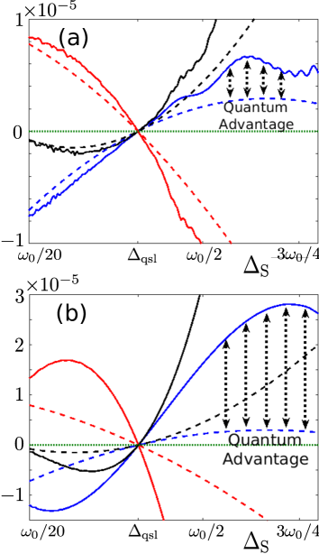
Figure 5: Quantum enhanced refrigeration: Power $\overline{\dot{W}}$ (black lines) and heat currents $\overline{J_{\rm h}}$ (red lines) and $\overline{J_{\rm c}}$ (blue lines) averaged over $n=10$ modulation periods (solid lines) as compared to the counterparts under Markovian approximation for long cycles, i.e., $n\to\infty$ (dashed lines), versus the modulation frequency $\Delta_{\rm S}$, for (a) quasi-Lorentzian spectral functions with $N=1,\delta=3,\epsilon=0.01,\alpha=1,\Gamma_{\rm B}=0.2$ (see Eq. (54)) and (b) super-Ohmic spectral functions with $s=2,\bar{\nu}=1,\delta=0.1,\epsilon=0.1,\alpha=1$ (see Eq. (55)). The enhanced overlap resulting from fast modulation (large $\Delta_{\rm S}$) enhances the heat currents $\overline{J_{\rm c}}$ to up to a factor larger than $2$ for (a) and larger than $9$ for (b) in the refrigerator regime (shown by dotted double-arrowed lines), signifying quantum advantage. The green dotted line corresponds to zero power and currents. Here $\lambda=0.2,\omega_{0}=20,\gamma_{0}=1,\beta_{\rm h}=0.001,\beta_{\rm c}=0.002$.

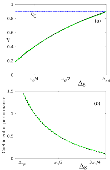
Figure 6: Efficiency and coefficient of performance (a) Efficiency $\eta$ for the heat engine in the anti-Zeno dynamics regime (green solid line), and the same in the long coupling time limit $\tau_{\rm C}\to\infty$ (black dashed line), versus the modulation frequency $\Delta_{\rm S}$, for $\beta_{\rm h}=0.0005$ and $\beta_{\rm c}=0.005$. The efficiency approaches the Carnot limit (blue dotted line) $\eta_{C}=1-\beta_{\rm h}/\beta_{\rm c}$ at $\Delta=\Delta_{\rm qsl}$. (b) Coefficient of performance for the refrigerator in the anti-Zeno dynamics regime (green solid line), and the same in the long time $t\to\infty$ limit (black dashed line), for $\beta_{\rm h}=0.001$ and $\beta_{\rm c}=0.002$. Here $\lambda=0.2,\omega_{0}=20$, and we consider thermal machines coupled to thermal baths with quasi-Lorentzian spectral functions with $N=1,\gamma_{0}=1,\delta=3,\epsilon=0.01,\alpha=1,\Gamma_{\rm B}=0.2$ (see Eq. (54)).

Quantum refrigeration: AZD can lead to quantum advantage in the refrigerator regime as well, for modulation rates beyond the quantum speed limit mukherjee16speed ; deffner17quantum (see App. A), by enhancing the heat current $\overline{J}_{\rm c}$, thus resulting in faster cooling of the cold bath. As for HE, numerical analysis shows that quasi-Lorentzian, as well as super-Ohmic bath spectral functions can lead to significant quantum advantage in the AZD regime (see Fig. 5). On the other hand, as for the efficiency in case of the HE, the coefficient of performance

$${\rm COP}=-\frac{\overline{J_{\rm c}}}{\overline{\dot{W}}}$$ (18)

is not significantly affected by the broadening of the sinc function, and on average remains identical to that obtained under slow modulation in the Markovian regime (see Fig. 6b and Methods “Efficiency and coefficient of performance”).

Discussion

We have explored the hitherto uncharted domain of quantum heat engines (QHEs) and refrigerator (QRs) based on quantum working fluids (WFs) intermittently coupled and decoupled from heat baths operating on non-Markovian time scales. We have shown that for driving (control) faster than the correlation (memory) time of the bath, one may achieve dramatic output power boost in the anti-Zeno dynamics (AZD) regime.

Let us revisit our findings, using as a benchmark the Markovian regime under periodic driving: In the latter regime, detailed balance of transition rates between the WF levels, as well as the periodic driving (modulation) rate, determine, according to the First and Second Laws of thermodynamics, the heat currents between the (hot and cold) baths, and thereby the power produced or consumed. In our present treatment, the Markovian regime is recovered under slow modulation, such that the WF-baths coupling duration $\tau_{\rm C}$ exceeds the bath correlation time $\tau_{\rm B}$. Then, the Markovian approximation is adequate for studying the operation of the QHE or the QR. By contrast, under fast modulations, such that $\tau_{\rm C}=n\tau_{\rm S}\lesssim\tau_{\rm B}$, the working fluid interacts with the baths over a broad frequency range of the order of $\sim\tau_{\rm C}^{-1}$, according to the time-energy uncertainty relation in quantum mechanics. The frequency-width over which system-bath energy exchange takes place can lead to anti-Zeno dynamics (AZD). The resultant quantum advantage is then especially pronounced for bath spectral functions that are appreciably shifted by $\delta>\Gamma_{\rm B}\sim\tau_{\rm B}^{-1}$, from the centers of the sinc functions that govern the system-bath energy exchange rates.

We have explicitly restricted the results to mutually symmetric bath spectral functions (e.g., the experimentally common Lorentzian or Gaussian spectra), in order to ensure time-independent steady-states of the WF. Yet this requirement is not essential, since the WF steady-state may be time-dependent as long as it is periodic so as to allow for cyclic operation. The AZD kofman01universal ; kofman04unified ; kofman00acceleration ; erez08 ; gordon09cooling ; gordon10equilibration ; alvarez10zeno ; gordon07universal can arise for any bath spectra of finite width $\sim 1/\tau_{\rm B}$, as long as $n\tau_{\rm S}\lesssim\tau_{\rm B}$. One can therefore operate a thermal machine provided stroke 1 of the cycle is in the AZD regime and achieve a quantum advantage without additional restrictions on the bath spectral functions (see Methods “Thermal machines with arbitrary (asymmetric) spectral functions”).

The QHM discussed here is driven by external modulation. As previously shown both theoretically kofman00acceleration ; kofman01universal ; kofman04unified ; gordon07universal ; erez08 ; gordon09cooling and experimentally alvarez10zeno ; almog11direct , periodic perturbations of the TLS state can increase its relaxation rate in the non-Markovian anti-Zeno regime. The reason for the power boost is that at the non-Markovian stage of the evolution which occurs on short time scales, the sinc factors in the convolutions with $G(\omega)$, as in (32), are sufficiently broad so as to modify the convolutions and hence the relaxation rates in (34) in comparison with the Markovian case, where these sinc functions are spectrally narrow enough to be approximated by delta-functions. Under the conditions chosen in the paper, this modification leads to an increase in the TLS relaxation rates and hence to a power boost. This boost is of quantum nature, since the broadening of the sinc factors is due to the quantum time-energy uncertainty relation that may lead to the violation of energy conservation at short times. The quantum mechanical time-energy uncertainty relation employed here reflects the fact that the Scrödinger equation for a two-level system coupled to a bath renders the energy transfer probability from the two-level system to the bath and back oscillatory in time. Such oscillation leads at short times (comparable to the required cycle period) to sinc-like deviation from delta-function energy conservation. Classical description of analogous processes, even beyond the Markovian approximation, does not involve discrete energy levels and hence no oscillations of the system-bath transfer rate that deviates from energy conservation. Thus, the effects discussed here are inherently quantum mechanical.

The non-Markovian effect in the present context is quantified by the spectral widths of the sinc functions compared to the bath-response $G(\omega)$ spectral width $1/\tau_{\rm B}$. If the cycle duration is kept fixed, then the non-Markovian effect scales with the spectral width of $G(\omega)$. Hence, super-Ohmic bath spectra with their salient cutoff provide realistic examples of the non-Markovian effects described here. Such bath spectra should be contrasted with the flatter and broader Ohmic spectra. Yet, non-Markovian dynamics does not necessarily imply a quantum advantage, as discussed in App. B.

The predicted power boost relies on transient dynamics: the heat fluxes change with time within $t=\tau_{C}$ in the non-Markovian AZD regime, even when the WF state hardly changes during that time interval. Yet it is essential that we incorporate this transient dynamics within steady-state cycles by decoupling the WF from the baths, allowing the bath-correlations to vanish within $\tau_{\rm B}$ and then recoupling the WF again to the baths when they have all resumed their initial states. These cycles can be repeated without restriction, thereby allowing us to operate the QHM with quantum enhanced performance even for long times, despite the reliance on transient dynamics within the stroke 1 of each cycle.

The quantum advantage of AZD, at zero energetic cost (see App. C), manifests itself in the form of higher output power, for the same efficiency, in the QHE regime ($\Delta_{\rm S}<\Delta_{\rm qsl}$), as compared to that obtained under Markovian dynamics in the limit of large $\tau_{\rm C}$, all other parameters remaining the same. Alternatively, in the QR regime ($\Delta_{\rm S}>\Delta_{\rm qsl}$), AZD may lead to quantum advantage over Markovian dynamics in the form of higher heat current $\overline{J}_{\rm c}$, or, equivalently, higher cooling rate of the cold bath, for the same coefficient of performance. The latter effect leads to the enticing possibility of quantum-enhanced speed-up of the cooling rate of systems as we approach the absolute zero, and raises questions regarding the validity of the Third Law of Thermodynamics in the quantum non-Markovian regime, if we expect the vanishing of the cooling rate at zero temperature as a manifestation of the Third Law kolar12 ; paz17 ; masanes17a .

The QHE power boost in the anti-Zeno regime results from a corresponding increase in the rates of heat-exchange and entropy production, arising from the TLS relaxation by both baths. This is the reason that the efficiency, i.e., the ratio of the work output to the heat input, is unchanged, i.e. is the same as in the standard Markovian regime. Yet, all parameters being equal, the QHM rate of operation (as measured by the power output) speeds up in the anti-Zeno regime, which constitutes a practical quantum advantage.

One can extend the analysis discussed here to Otto cycles mukherjee16speed ; kosloff17the : Fast periodic modulation during the non-unitary strokes of an Otto cycle can speed up the thermalization through AZD, thereby allowing quantum enhanced performance. Interestingly, fast modulation in the Otto cycle can yield enhanced power or refrigeration rate, even in the Markovian regime erdman18maximum .

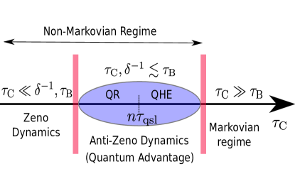
Figure 7: Dynamical regimes: Schematic display of the different regimes of operation, as a function of the working fluid (system) - baths coupling duration $\tau_{\rm C}$.

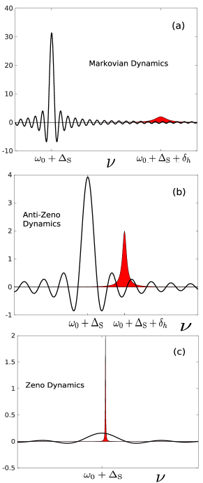
Figure 8: Spectral and sinc functions: The quasi-Lorentzian spectral function $G_{h}(\nu)$ (red filled curve) and ${\rm sinc}\left[\left(\nu-\omega_{0}-\Delta\right)t\right]$ (black solid curve) at time $t=10\tau_{\rm S}$ for (a) Markovian dynamics with $\Delta_{\rm S}=10\Gamma_{\rm B}$, (b) anti-Zeno dynamics with $\Delta_{\rm S}=80\Gamma_{\rm B}$ and (c) Zeno dynamics with $\Delta_{\rm S}=2000\Gamma_{\rm B}$. The overlap between the two functions is maximal for anti-Zeno dynamics, while it vanishes both for slow modulation, when the sinc function is narrow, as well as for Zeno dynamics, when the sinc function is much broader than $G_{h}(\nu)$, and approaches zero for all $\nu$. The same $G_{h}(\nu)$ is considered in (a), (b) and (c). Here $\omega_{0}=20,\gamma_{0}=1,\Gamma_{\rm B}=0.2,N=1,\delta_{\rm h}=3,\epsilon=0.01,\alpha=1$.

Finally, in the regime of ultrafast modulation with $\tau_{\rm C}^{-1}\gg\Gamma_{\rm B},\delta$, quantum Zeno dynamics sets in, leading to vanishing heat currents and power, thus implying that such a regime is incompatible with thermal machine operation (see Fig. 7, App. B and Fig. 8). While Zeno dynamics has commonly been associated with measurements misra77the ; kofman00acceleration ; itano90quantum ; kofman01zeno , both the Zeno and the anti-Zeno effects occur under various frequent perturbations, such as phase flips and nonselective (unread) measurements. Generally speaking, to observe the discussed effects, it is sufficient to repeatedly perform cycles of coupling the system (here - the WF) with another system (here - a bath), then destroying or sharply changing the coherence between the two. This sharp change can be effected in different ways, e.g., by a measurement of the system (which can be read-out or not) or, as in our case, by abruptly decoupling the WF and the baths, which gives rise to Zeno or anti-Zeno dynamics kofman01universal ; kofman04unified ; kofman00acceleration ; erez08 ; gordon09cooling ; gordon10equilibration . In contrast to previous studies, here the Zeno or anti-Zeno dynamics of the WF arises by an external periodic field, and therefore not around the frequency $\omega_{0}$ of the unperturbed system, as in previous cases, but at multiple sideband frequencies $\omega_{0}+q\Delta_{\rm S}$.

The Markovian approximation suffices to find the correct efficiency (for a QHE) or the coefficient of performance (for a QR), even in the non-Markovian regimes, for mutually symmetric bath spectral functions (see Eq. (10)). This guarantees that the efficiency always remains below the Carnot bound, even under fast modulations (see Fig. 6).

Our scenario is conceptually different from that in which work is produced by a QHE on an external quantum system and quantum effects arise from the interaction between the quantum WF and the external quantum system watanabe17quantum . Such quantum effects are absent in our case, where work input in the QHE is provided by a classical field.

Experimental scenarios where the predicted AZD quantum advantage may be tested are diverse. Since non-Markovianity in general, and AZD in particular, require non-flat bath spectral functions, suitable candidates for the hot and cold baths are microwave cavities and waveguides in which dielectric gratings are embedded, with distinct cut-off and bandgap frequencies magnusson92new ; klimovsky15 and the WF is a qubit whose level distance is modulated by fields. The required qubit modulations are then compatible with MHz periodic driving of superconducting transmon qubits Houck08controlling ; Peterer15coherence or NV-center qubits in diamonds sangtawesin14fast . One can effectively decouple the WF from the thermal baths in stroke 2 by abruptly changing the resonance frequency of the two-level WF from $\omega_{0}$ to $\tilde{\omega}$, thus rendering the WF strongly off-resonant with the thermal baths, so that $G_{\rm h}\left(\tilde{\omega}\right)\approx G_{\rm c}\left(\tilde{\omega}\right)=0$), thereby precluding any energy flow between the baths and the WF. We can recouple the WF with the thermal baths by reverting this frequency back to $\omega_{0}$, and then modulating it periodically, so as to generate either Markovian or non-Markovian anti-Zeno dynamics, as discussed above alvarez10zeno .

The AZD regime was experimentally observed in NMR setups alvarez10zeno . Micro/nano-scale heat machines have been experimentally realized, for a trapped calcium ion as the WF rossnage16a ; nano-mechanical oscillators WF powered by squeezed thermal bath klaers17squeezed ; atomic heat machines assisted by quantum coherence klatzow19experimental ; or a nuclear spin $1/2$ as the WF in a quantum Otto cycle peterson18experimental .

The novel effects and performance trends of QHE and QR in the non-Markovian time domain, particularly the anti-Zeno induced power boost, open new, dynamically-controlled pathways in the quest for genuine quantum features in heat machines, which has been a major motivation of quantum thermodynamics in recent years ghosh17catalysis ; ghosh2018thermodynamic ; scully03extracting ; fialko12isolated ; berut12experimental ; rossnage14nanoscale ; uzdin15equivalence ; klaers17squeezed ; klimovsky18single ; niedenzu18quantum ; ghosh18we ; binder18book .

Methods

Floquet Analysis of the non-Markovian Master Equation. Let us consider the differential non-Markovian master equation for the system density operator $\rho_{\rm S}(t)$ in the interaction picture kofman04unified :

$$\dot{\rho}_{\rm S}(t) = -\int^{t}_{0}ds{\rm Tr}_{\rm B}\big{[}\hat{S}(t)\otimes\hat{B}_{\rm c}(t)$$ (19)

$$+ \hat{S}(t)\otimes\hat{B}_{\rm h}(t),[\hat{S}(s)\otimes\hat{B}_{\rm c}(s)$$

$$+ \hat{S}(s)\otimes\hat{B}_{\rm h}(s),\rho_{\rm S}(t)\otimes\rho_{\rm B}]\big{]}.$$

Here $\rho_{\rm B}=\rho_{\rm Bc}\otimes\rho_{\rm Bh}$, where $\rho_{{\rm B}j}$ is the density operator of bath $j$. In the derivation of Eq. (19) we have assumed that Tr$[\hat{B}_{j},\rho_{{\rm B}j}]=0$. We consider commuting bath operators $\left[\hat{B}_{\rm c}(t),\hat{B}_{\rm h}(t^{\prime})\right]=0$, such that the two baths act additively in Eq. (19). Below we focus on only one of the baths and omit the labels $c/h$ for simplicity. We then have

$$\hat{S}^{\dagger}(t) = \hat{S}(t)$$

$$\hat{B}^{\dagger}(t) = \hat{B}(t)$$

$${\rm Tr}\left[\hat{B}(t)\hat{B}(s)\rho_{\rm B}\right] = \langle\hat{B}(t)\hat{B}(s)\rangle\equiv\Phi(t-s)$$

$$\hat{S}(t) = \sum_{q,\omega}S_{q,\omega}e^{-i(\omega+q\Delta_{\rm S})t}.$$ (20)

where $q$ are integers and $\omega$ are transition frequencies of the system $\mathcal{S}$.

One can use Eq. (20) to write the first term on the r.h.s. of Eq. (19) as

$$T_{1} = -\sum_{\omega,\omega^{\prime},q,q^{\prime}}e^{i[(\omega^{\prime}-\omega)+(q^{\prime}-q)\Delta_{\rm S}]t}\hat{S}^{\dagger}_{q^{\prime},\omega^{\prime}}\hat{S}_{q,\omega}\rho_{\rm S}(t)$$ (21)

$$\times \int^{t}_{0}\big{[}\Phi(t-s)e^{i(\omega+q\Delta_{\rm S})(t-s)}\big{]}ds.$$

In the limit of times of interest, i.e., times larger than the period of driving $\tau_{\rm S}$ and the effective periods of the system, $t\gg\tau_{\rm S},(\omega+q\Delta_{\rm S})^{-1}$, the terms with the fast oscillating factor before the integral in Eq. (21) become small and can be neglected, i.e., the secular approximation becomes applicable, such that

$$\left(q^{\prime}-q\right)\Delta_{\rm S} = \omega-\omega^{\prime},$$ (22)

which generally holds only for

$$\omega^{\prime} = \omega;\leavevmode\nobreak\ \leavevmode\nobreak\ q^{\prime}=q,$$ (23)

as long as $\left(q^{\prime}-q\right)\Delta_{\rm S}$ is not close to $\left(\omega^{\prime}-\omega\right)$ for any $q,q^{\prime},\omega,\omega^{\prime}$. Condition (23) gives us

$$T_{1} \approx -\sum_{\omega,q}\hat{S}^{\dagger}_{q,\omega}\hat{S}_{q,\omega}\rho_{\rm S}(t)$$ (24)

$$\int^{t}_{0}\big{[}\Phi(t-s)e^{i(\omega+q\Delta_{\rm S})(t-s)}\big{]}ds$$

$$= -\sum_{\omega,q}\hat{S}^{\dagger}_{q,\omega}\hat{S}_{q,\omega}\rho_{\rm S}(t)\int^{t}_{0}\big{[}\Phi(\mu)e^{i(\omega+q\Delta_{\rm S})\mu}\big{]}d\mu$$

$$= -\sum_{\omega,q}\hat{S}^{\dagger}_{q,\omega}\hat{S}_{q,\omega}\rho_{\rm S}(t)$$

$$\times \int_{-\infty}^{\infty}G(\nu)\int^{t}_{0}e^{-i\left[\nu-\left(\omega+q\Delta_{\rm S}\right)\right]\mu}d\mu d\nu,$$

where $\mu=t-s$, and

$$\Phi(\mu)=\int_{-\infty}^{\infty}d\nu G(\nu)e^{-i\nu\mu}.$$ (25)

In the limit of slow modulation, such that $t=n\tau_{\rm S}\gg\tau_{\rm B}$, one can perform the Markov approximation, thereby extending the upper limit of the integral in time in Eq. (24) to $t\to\infty$, which finally results in the time-independent Markovian form breuer02

$$T_{1} \approx -\pi\sum_{\omega,q\geq 0}\hat{S}^{\dagger}_{q,\omega}\hat{S}_{q,\omega}\rho_{\rm S}(t)G(\omega,q).$$ (26)

On the other hand, in the limit of $t\sim n\tau_{\rm S}\lesssim\tau_{\rm B}$, the Markovian approximation becomes invalid, and one gets

$$T_{1} \approx -\sum_{\omega,q}\hat{S}^{\dagger}_{q,\omega}\hat{S}_{q,\omega}\rho_{\rm S}(t)\int_{-\infty}^{\infty}d\nu G(\nu)$$ (27)

$$\Big{[}\frac{\sin\left(\left[\nu-\left(\omega_{0}+q\Delta_{\rm S}\right)\right]t\right)}{\nu-\left(\omega_{0}+q\Delta\right)}$$

$$+ i\left(\frac{\cos\left(\left[\nu-\left(\omega_{0}+q\Delta_{\rm S}\right)\right]t\right)-1}{\nu-\left(\omega_{0}+q\Delta_{\rm S}\right)}\right)\Big{]}.$$

Progressing similarly as above, one can arrive at similar expressions for other terms in Eq. (19) as well.

Non-Markovian dynamics of a driven two-level system in a dissipative bath. The non-Markovian master equation followed by the TLS WF subjected to the Hamiltonian Eq. (6) is (see Eq. (19))

$$\mathcal{L}\left[{\rho}_{s}(t)\right] = \left[\left(A_{\downarrow}+\bar{A}_{\downarrow}\right)\sigma^{+}\rho_{s}(t)\sigma^{-}-A_{\downarrow}\sigma^{-}\sigma^{+}\rho_{s}(t)-\bar{A}_{\downarrow}\rho_{s}(t)\sigma^{-}\sigma^{+}\right]$$ (28)

$$+ \left[\left(A_{\uparrow}+\bar{A}_{\uparrow}\right)\sigma^{-}\rho_{s}(t)\sigma^{+}-A_{\uparrow}\sigma^{+}\sigma^{-}\rho_{s}(t)-\bar{A}_{\uparrow}\rho_{s}(t)\sigma^{+}\sigma^{-}\right]+M\sigma^{-}\rho_{s}(t)\sigma^{-}+\bar{M}\sigma^{+}\rho_{s}(t)\sigma^{+},$$

where we have removed the $h,c$ indices for simplicity, and considered the dynamics due to a single bath. Here

$$A_{\downarrow} = \sum_{q,q^{\prime}\in\mathbb{Z}}\xi(q^{\prime})\overline{\xi}(q)e^{i\left(q-q^{\prime}\right)\Delta_{\rm S}t}\int^{\infty}_{-\infty}G(\nu)\int^{t}_{0}e^{-i\left[\nu-\left(\omega_{0}+q\Delta_{\rm S}\right)\right]\tau}d\nu d\tau,$$

$$A_{\uparrow} = \sum_{q,q^{\prime}\in\mathbb{Z}}\overline{\xi}(q^{\prime})\xi(q)e^{-i\left(q-q^{\prime}\right)\Delta_{\rm S}t}\int^{\infty}_{-\infty}G(\nu)\int^{t}_{0}e^{-i\left[\nu+\left(\omega_{0}+q\Delta_{\rm S}\right)\right]\tau}d\nu d\tau,$$

$$M = \sum_{q,q^{\prime}\in\mathbb{Z}}\xi(q)\xi(q^{\prime})e^{-i\left[2\omega_{0}+\left(q+q^{\prime}\right)\Delta_{\rm S}\right]t}\int^{\infty}_{-\infty}G(\nu)\left(\int^{t}_{0}e^{i\left[\nu-\left(\omega_{0}+q\Delta_{\rm S}\right)\right]\tau}d\tau+\int^{t}_{0}e^{-i\left[\nu+\left(\omega_{0}+q\Delta_{\rm S}\right)\right]\tau}d\tau\right)d\nu,$$

$$\sigma_{x}(t) = \sum_{q\in\mathbb{Z}}\left(\xi(q)e^{-i\left(\omega_{0}+q\Delta_{\rm S}\right)t}\sigma^{-}+\overline{\xi}(q)e^{i\left(\omega_{0}+q\Delta_{\rm S}\right)t}\sigma^{+}\right),$$

$$\xi(q) = \frac{1}{\tau_{\rm S}}\int_{0}^{\tau_{\rm S}}e^{i\int^{t}_{0}\lambda\Delta_{\rm S}\sin\left(\Delta_{\rm S}t^{\prime}\right)dt^{\prime}}e^{iq\Delta_{\rm S}t}dt$$ (29)

$\bar{A}_{\downarrow}$, $\bar{A}_{\uparrow}$ and $\bar{M}$ are the complex conjugates of $A_{\downarrow}$, $A_{\uparrow}$ and $M$, respectively. The terms corresponding to $\sigma^{\pm}\rho_{\rm S}(t)\sigma^{\pm}$ in Eq. (28) vanish for diagonal steady-state $\rho_{\rm S}(t)\to\rho_{\rm ss}$ (see Eq. (11)). Here we focus on times longer than several modulation periods, i.e., $t=n\tau_{\rm S}\gg\tau_{\rm S}$, when the fast oscillatory terms corresponding to $q\neq q^{\prime}$ vanish as well, such that

$$A_{\downarrow} \approx \sum_{q}P_{q}\int^{\infty}_{-\infty}G(\nu)\int^{t}_{0}e^{-i\left[\nu-\left(\omega_{0}+q\Delta_{\rm S}\right)\right]\tau}d\nu d\tau,$$

$$A_{\uparrow} \approx \sum_{q}P_{q}\int^{\infty}_{-\infty}G(\nu)\int^{t}_{0}e^{-i\left[\nu+\left(\omega_{0}+q\Delta_{\rm S}\right)\right]\tau}d\nu d\tau,$$

$$P_{q} = |\xi(q)|^{2}.$$ (30)

We note that

$$\int^{t}_{0}e^{\pm i\left[\nu\pm\left(\omega_{0}+q\Delta_{\rm S}\right)\right]\tau}d\tau=\frac{\sin\left(\left[\nu\pm\left(\omega_{0}+q\Delta_{\rm S}\right)\right]t\right)}{\nu\pm\left(\omega_{0}+q\Delta_{\rm S}\right)}$$ (31)

$$\mp i\left[\frac{\cos\left(\left[\nu\pm\left(\omega_{0}+q\Delta_{\rm S}\right)\right]t\right)-1}{\nu\pm\left(\omega_{0}+q\Delta_{\rm S}\right)}\right].$$

The imaginary part in Eq. (31) acts on terms of the form $i{\rm Im}[\tilde{\mathcal{I}}_{j}\left(\pm\omega_{q},t\right)]\left(\sigma^{\mp}\sigma^{\pm}\rho_{\rm S}(t)-\rho_{\rm S}(t)\sigma^{\mp}\sigma^{\pm}\right)$, which vanish at large times when the off-diagonal elements $\rho_{\rm S}(t)$ approach zero for any initial state. On the other hand, the real part of Eq. (31) gives rise to terms of the form

$$\mathcal{I}_{j}\left(\pm\omega_{q},t\right) := {\rm Re}[\tilde{\mathcal{I}}_{j}\left(\pm\omega_{q},t\right)]$$ (32)

$$= \int^{\infty}_{-\infty}G_{j}(\nu)\frac{\sin\left(\left[\nu\mp\left(\omega_{0}+q\Delta_{\rm S}\right)\right]t\right)}{\nu\mp\left(\omega_{0}+q\Delta_{\rm S}\right)}d\nu,$$

In the limit of slow modulation such that $t\sim n\tau_{\rm S}\gg\tau_{\rm B}$ ($n\in\mathbb{Z},\leavevmode\nobreak\ n\gg 1$), the function $\sin\left(\left[\nu\pm\left(\omega_{0}+q\Delta_{\rm S}\right)\right]t\right)/\left[\nu\pm\left(\omega_{0}+q\Delta_{\rm S}\right)\right]$ assumes a delta function centred at $\nu=\pm\left(\omega_{0}+q\Delta_{\rm S}\right)$, thus leading to the familiar Markovian form of master equation, with

$$\mathcal{I}_{j}\left(\pm\omega_{q},t\right)=\pi G_{j}\left[\pm\left(\omega_{0}+q\Delta_{\rm S}\right)\right]\leavevmode\nobreak\ \leavevmode\nobreak\ \forall\leavevmode\nobreak\ t.$$ (33)

On the other hand, in the anti-Zeno regime of fast modulation: $t\sim n\tau_{\rm S}\lesssim\tau_{\rm B}$, $\mathcal{I}_{j}\left(\pm\omega_{q},t\right)$ is not given by Eq. (33), and one needs to consider the full form Eq. (32).

In particular, for a diagonal state $\rho_{\rm S}(t)=p_{1}(t)|1\rangle\langle 1|+p_{1}(t)|0\rangle\langle 0|$, the dynamics Eq. (28) - Eq. (32) leads us to the rate equations

$$\dot{p}_{1}(t) = -\dot{p}_{0}(t)=R_{0}(t)p_{0}(t)-R_{1}(t)p_{1}(t)$$

$$R_{0}(t) = \frac{\lambda^{2}}{4}\left[\mathcal{I}_{\rm h}(-\omega_{0}-\Delta_{\rm S},t)+\mathcal{I}_{\rm c}(-\omega_{0}+\Delta_{\rm S},t)\right]$$

$$R_{1}(t) = \frac{\lambda^{2}}{4}\left[\mathcal{I}_{\rm h}(\omega_{0}+\Delta_{\rm S},t)+\mathcal{I}_{\rm c}(\omega_{0}-\Delta_{\rm S},t)\right]$$ (34)

In the Zeno regime of ultra-fast modulation, obtained in the limit of $t\sim n\tau_{\rm S}\ll\tau_{\rm B}$, the integral $\mathcal{I}(\omega_{q},t)$ vanishes (see Fig. 8), thus leading to the Zeno effect of no dynamics.

Equations (19), (24) and (28) are of the type known as the differential master equation (DME). An alternative approach is based on the (less convenient) integro-differential master equation (IME). The two equations are mathematically different and hence require different procedures for reducing them to the Markovian master equation (MME). However, the IME and the DME have the same validity conditions, i.e., generally similar accuracy. The IME and the DME follow from the exact expansions in the totally ordered and partially ordered cumulants, respectively, upon neglecting terms of order higher than $2$ in the system-bath coupling, which determines their accuracy breuer02 ; kofman90non ; gordon07universal

The rates (34) can be negative when the modulation (or measurement) period is short enough to break the rotating wave approximation (RWA). Yet the probabilities ${p}_{0}(t)$, ${p}_{1}(t)$ are never negative, as detailed in Refs. gordon07universal ; erez08 and concisely proven in the next section.

Non-Markovian master equation with non-negative probabilities. The non-Markovian master equations (MEs) for an arbitrarily driven (controlled) two-level system (TLS) presented in (34) have been derived and discussed in Refs. kofman00acceleration ; kofman01universal ; kofman04unified ; erez08 ; gordon09cooling and experimentally verified in Refs. alvarez10zeno ; almog11direct . These MEs involve the time-dependent relaxation rates $R_{0}(t)$ and $R_{1}(t)$ which can take negative values, since the quantities ${\cal I}_{j}$, (32), are convolutions of a positive spectral response function $G_{j}(\nu)$ with a sinc function which takes positive or negative values. As a result, the solutions of the MEs for the populations (probabilities) $p_{0}(t)$ and $p_{1}(t)$ of the TLS levels are not guaranteed to be non-negative, i.e., to satisfy

$$0\leq p_{k}(t)\leq 1\quad(k=0,1).$$ (35)

Below we show that the inequalities (35) hold, at least, up to second order in the system-bath coupling strength. This means that for a weak coupling, violations of (35) (if any) are negligibly small.

First, we note that at sufficiently long times, $t\gg\tau_{\rm B}$, the MEs become Markovian and coincide with the Lindblad equation. In this case, the rates are constant and positive, $R_{0},R_{1}\geq 0$, as follows from (33). The inequalities (35) are now known to hold. Generally, the MEs are valid if the couplings of the TLS with the baths are sufficiently weak, so that

$$R_{0}\tau_{\rm B}\ll 1,\quad R_{1}\tau_{\rm B}\ll 1.$$ (36)

Consider now the short times, $t\lesssim\tau_{\rm B}$, where the non-Markovian effects are important. Since $p_{0}(t)+p_{1}(t)=1$, we rewrite

$$p_{0}(t)=\frac{1-w(t)}{2},\quad p_{1}(t)=\frac{1+w(t)}{2},$$ (37)

where $w(t)=p_{1}(t)-p_{0}(t)$ is the TLS population inversion. In terms of $w(t)$, inequalities (35) are equivalent to

$$-1\leq w(t)\leq 1,$$ (38)

which we now prove.

The condition (36) implies that at times $\lesssim\tau_{\rm B}$, the relaxation can be approximated to first order in the relaxation rates. In this approximation, (34) yields

$$w(t)=w(0)[1-J_{+}(t)]+J_{-}(t),$$ (39)

where

$$J_{\pm}(t)=J_{0}(t)\pm J_{1}(t)$$ (40)

and

$$J_{k}(t)=\int_{0}^{t}d\tau R_{k}(\tau)\quad\quad(k=0,1).$$ (41)

From (32) and (34), one can check that

$$J_{0}(t),J_{1}(t)\geq 0.$$ (42)

From (39) we obtain

$$|w(t)| \leq|w(0)|[1-J_{+}(t)]+|J_{-}(t)|$$ (43)

$$\leq 1-J_{+}(t)+J_{+}(t)=1,$$

yielding (38). The second inequality in (43) follows from the assumption $|w(0)|\leq 1$ and the relation $|J_{-}(t)|\leq J_{+}(t)$, resulting from (40) and (42).

Steady states in the anti-Zeno dynamics regime. Now we study the regimes which allow us to operate the setup with a time-independent steady state $\rho_{\rm ss}$ even inside the AZD regime. We note that for $t\to\infty$, $I_{j}\left(\omega_{q},t\right)$ reduces to the time-independent form $\pi G_{j}(\omega_{q})$, thus leading us to the Eq. (11).

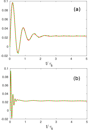
Figure 9: Dissipation rates: The time dependent rates $\mathcal{I}_{\rm h}(\omega_{0}+\Delta_{\rm S},t)$ (magenta solid line) and $\mathcal{I}_{\rm c}(\omega_{0}-\Delta_{\rm S},t)$ (turquoise dashed line) as a function of time-periods $t/\tau_{\rm S}$ for spectral functions Eq. (54) with $\delta=4.5$ for (a) $\tau_{\rm S}=2\pi/\Delta_{\rm S}=2$ and (b) $\tau_{\rm S}=2\pi/\Delta_{\rm S}=10$. As explained in Methods “Steady states in the anti-Zeno dynamics regime”, symmetric spectral functions $G_{\rm h}(\omega+x)=G_{\rm c}(\omega_{0}-x)$ for real $x$ lead to $\mathcal{I}_{\rm h}(\omega_{0}+\Delta_{\rm S},t)=\mathcal{I}_{\rm c}(\omega_{0}-\Delta_{\rm S},t)$. A fast modulation ($\tau_{\rm S}=2$) results in oscillating and time-dependent $\mathcal{I}_{\rm h,c}(t)$ for large $t/\tau_{\rm S}$, while slow modulation ($\tau_{\rm S}=10$) leads to an approximately constant $\mathcal{I}_{\rm h,c}$ even for small $t/\tau_{\rm S}$ Here $\omega_{0}=10,\gamma_{0}=1,\Gamma_{\rm B}=1$.

On the other hand, for $t\sim n\tau_{\rm S}\lesssim\tau_{\rm B}$, $I_{j}\left(\omega_{q},t\right)$ includes contributions from $G_{j}(\omega_{q}+\nu)$, where

$$|\nu|\lesssim 1/t=1/\left(n\tau_{\rm S}\right).$$ (44)

Further, we consider $\omega_{0}$, $T_{\rm c},T_{\rm h}$, and $\Delta_{\rm S}<\omega_{0}$ large enough, such that $1/t\ll\omega_{0}\pm\Delta_{\rm S},T_{\rm c},T_{\rm h}$. Therefore in this limit the KMS condition gives us

$$G_{j}\left(-\left(\omega_{q}+\nu\right)\right) \approx e^{-\left(\omega_{q}+\nu\right)\beta_{j}}G_{j}\left(\omega_{q}+\nu\right)$$ (45)

$$\approx e^{-\omega_{q}\beta_{j}}G\left(\omega_{q}+\nu\right).$$

This immediately leads us to

$$\mathcal{I}_{j}(-\omega_{q},t) \approx e^{-\omega_{q}\beta_{j}}\mathcal{I}_{j}(\omega_{q},t),$$ (46)

and consequently (see Eq. (11))

$$w \approx \frac{e^{-\left(\omega_{0}+\Delta_{\rm S}\right)\beta_{\rm h}}\mathcal{I}_{\rm h}\left(\omega_{0}+\Delta_{\rm S},t\right)}{\mathcal{I}_{\rm h}\left(\omega_{0}+\Delta_{\rm S},t\right)+\mathcal{I}_{\rm c}\left(\omega_{0}-\Delta_{\rm S},t\right)}$$ (47)

$$+ \frac{e^{-\left(\omega_{0}-\Delta_{\rm S}\right)\beta_{\rm c}}\mathcal{I}_{\rm c}\left(\omega_{0}-\Delta_{\rm S},t\right)}{\mathcal{I}_{\rm h}\left(\omega_{0}+\Delta_{\rm S},t\right)+\mathcal{I}_{\rm c}\left(\omega_{0}-\Delta_{\rm S},t\right)},$$

where we have considered the two sidebands $q=1,-1$ only.

The condition

$$\mathcal{I}_{\rm h}\left(\omega_{0}+\Delta_{\rm S},t\right)\approx\alpha\mathcal{I}_{\rm c}\left(\omega_{0}-\Delta_{\rm S},t\right),$$ (48)

which holds for mutually symmetric bath spectral functions up to a multiplicative factor $G_{\rm h}(\omega_{0}+x)\approx\alpha G_{\rm c}(\omega_{0}-x)$ for any real $x$ and positive $\alpha$ (see Fig. 9), leads to the time-independent steady state $\rho_{\rm ss}$ with (see Eq. (11))

$$w\approx\frac{\alpha e^{-\left(\omega_{0}+\Delta_{\rm S}\right)\beta_{\rm h}}+e^{-\left(\omega_{0}-\Delta_{\rm S}\right)\beta_{\rm c}}}{\alpha+1}.$$ (49)

Efficiency and coefficient of performance.  The efficiency in the heat engine regime is given by

$$\eta=\frac{\oint_{\tau_{\rm C}}\left[J_{\rm h}(t)+J_{\rm c}(t)\right]dt}{\oint_{\tau_{\rm C}}J_{\rm h}(t)dt}=\frac{\left(\omega_{0}+\Delta_{\rm S}\right)\zeta_{\rm h}\oint_{\tau_{\rm C}}\mathcal{I}_{\rm h}(\omega_{0}+\Delta_{\rm S},t)dt+\left(\omega_{0}-\Delta_{\rm S}\right)\zeta_{\rm c}\oint_{\tau_{\rm C}}\mathcal{I}_{\rm c}(\omega_{0}-\Delta_{\rm S},t)dt}{\left(\omega_{0}+\Delta_{\rm S}\right)\zeta_{\rm h}\oint_{\tau_{\rm C}}\mathcal{I}_{\rm h}(\omega_{0}+\Delta_{\rm S},t)dt},$$

while the coefficient of performance in the refrigerator regime takes the form

$${\rm COP}=\frac{\oint_{\tau_{\rm C}}J_{\rm c}(t)dt}{{\oint_{\tau_{\rm C}}\left[J_{\rm h}(t)+J_{\rm c}(t)\right]dt}(t)}=\frac{\left(\omega_{0}-\Delta_{\rm S}\right)\zeta_{\rm c}\oint_{\tau_{\rm C}}\mathcal{I}_{\rm c}(\omega_{0}-\Delta_{\rm S},t)dt}{\left(\omega_{0}+\Delta_{\rm S}\right)\zeta_{\rm h}\oint_{\tau_{\rm C}}\mathcal{I}_{\rm h}(\omega_{0}+\Delta_{\rm S},t)dt+\left(\omega_{0}-\Delta_{\rm S}\right)\zeta_{\rm c}\oint_{\tau_{\rm C}}\mathcal{I}_{\rm c}(\omega_{0}-\Delta_{\rm S},t)dt},$$

where we have defined

$$\zeta_{\rm h}=\frac{e^{-(\omega_{0}+\Delta_{\rm S})\beta_{\rm h}}-w}{w+1},$$

$$\zeta_{\rm c}=\frac{e^{-(\omega_{0}-\Delta_{\rm S})\beta_{\rm c}}-w}{w+1}.$$ (50)

One can get the results of the Markovian ($\tau_{\rm C}\to\infty$) limit by replacing $\mathcal{I}_{j}(-\omega_{q},t)$ by $G_{j}\left(\omega_{q}\right)$.

Let us consider the integral:

$$\mathcal{I}_{\rm h}(\omega_{0}+\Delta_{\rm S},t) = \int^{\infty}_{-\infty}G_{\rm h}(\nu)\frac{\sin\left(\left[\nu-\left(\omega_{0}+\Delta_{\rm S}\right)\right]t\right)}{\nu-\left(\omega_{0}+\Delta_{\rm S}\right)}d\nu$$ (51)

$$\approx \int_{-\Delta_{\rm S}}^{\infty}G_{\rm h}(\omega_{0}+\Delta_{\rm S}+x)\frac{\sin\left(xt\right)}{x}dx,$$

where we have defined the variable $x=\nu-\left(\omega_{0}+\Delta_{\rm S}\right)$, and taken into account that $G_{\rm h}(\nu)=0$ for $0<\nu\leq\omega_{0}$ (see Eq. (8)), and $\sin\left(xt\right)/x$ is small for large $|x|$.

Similarly, we have

$$\mathcal{I}_{\rm c}(\omega_{0}-\Delta_{\rm S},t) = \int^{\infty}_{-\infty}G_{\rm c}(\nu)\frac{\sin\left(\left[\nu-\left(\omega_{0}-\Delta_{\rm S}\right)\right]t\right)}{\nu-\left(\omega_{0}-\Delta_{\rm S}\right)}d\nu$$ (52)

$$\approx \int_{-\Delta_{\rm S}}^{\infty}G_{\rm c}(\omega_{0}-\Delta_{\rm S}-y)\frac{\sin\left(yt\right)}{y}dy,$$

where $y=\left(\omega_{0}-\Delta_{\rm S}-\nu\right)$, and we have taken into account that $G_{\rm c}(\nu)=0$ for $\nu\geq\omega_{0}$ (see Eq. (8)), and $\sin\left(yt\right)/y$ is small for large $|y|$.

Clearly, for bath spectral functions related by Eq. (10), we have $\mathcal{I}_{\rm h}(-\omega_{0}-\Delta_{\rm S},t)\approx\alpha\mathcal{I}_{\rm c}(-\omega_{0}+\Delta_{\rm S},t)$, which in turn results in the efficiency and the coefficient of performance in the non-Markovian anti-Zeno dynamics regime being approximately equal to those in the Markovian dynamics regime (see Fig. 6).

Quasi-Lorentzian bath spectral functions. We focus on baths characterized by the spectral functions:

$$G_{\rm h}(\nu\geq 0) = \frac{1}{N}\sum_{r=1}^{N}\left[c_{r}\frac{\alpha\gamma_{0}\Gamma_{{\rm B},r}^{2}\Theta(\nu-\omega_{0}-\epsilon)}{(\omega_{0}+\Delta_{\rm S}+\delta_{r}-\nu)^{2}+\Gamma_{\rm B,r}^{2}}\right],$$

$$G_{\rm c}(\nu\geq 0) = \frac{1}{N}\sum_{r=1}^{N}\left[c_{r}\frac{\gamma_{0}\Gamma_{{\rm B},r}^{2}\Theta(\omega_{0}-\epsilon-\nu)\Theta(\nu-\epsilon)}{(\omega_{0}-\Delta_{\rm S}-\delta_{r}-\nu)^{2}+\Gamma_{\rm B,r}^{2}}\right]$$

$$G_{\rm h,c}(-\nu) = G_{\rm h,c}(\nu)e^{-\nu\beta_{\rm h,c}},$$ (53)

where we have considered the KMS condition, $\Theta$ is the step function, $N\in\mathbb{Z},\leavevmode\nobreak\ N>0$ denotes the number of peaks and $\Gamma_{{\rm B},r}=1/\tau_{{\rm B},r}>0$ is the width of the $r$-th peak. $\delta_{r}$ are the (real) Lamb self energy shifts, such that $G_{\rm h}$ ($G_{\rm c}$) is peaked at $\nu=\omega_{0}+\Delta+\delta_{r}$ ($\nu=\omega_{0}-\Delta-\delta_{r}$).

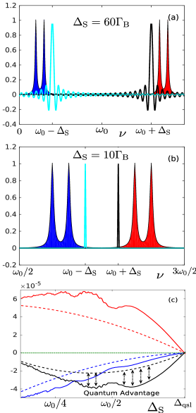
Figure 10: Quantum advantage with double-peaked spectral functions: Double-peaked spectral functions $G_{\rm h}(\nu)$ (red filled curve) and $G_{\rm c}(\nu)$ (blue filled curve), and the sinc functions ${\rm sinc}\left[\left(\nu-\omega_{0}-\Delta\right)t\right]$ (black solid curve) and ${\rm sinc}\left[\left(\nu-\omega_{0}+\Delta\right)t\right]$ (blue solid curve) for (a) fast modulation $\Delta_{\rm S}=60\Gamma_{\rm B}$ and (b) slow modulation $\Delta_{\rm S}=10\Gamma_{\rm B}$ at $t=10\tau_{\rm S}$. Fast (slow) modulation results in broadening (narrowing) of the sinc functions, thus leading to enhanced (reduced) overlap with the spectral functions. (c) Power $\overline{\dot{W}}$ (black lines) and heat currents $\overline{J_{\rm h}}$ (red lines) and $\overline{J_{\rm c}}$ (blue lines) averaged over $n=10$ modulation periods (solid lines) and the same obtained under the Markovian approximation for long cycles ($n\to\infty$) (dashed lines), versus the modulation frequency $\Delta_{\rm S}$. A significant quantum advantage (shown by dotted double-arrow lines) is obtained for fast modulation, when broadening of the sinc functions yields an output power boost by a factor greater than $2$ in the heat engine regime. The green dotted line corresponds to zero power and currents. Here $\lambda=0.2,\omega_{0}=20,N=2,\delta_{1}=2,\delta_{2}=4,\alpha=1,\gamma_{0}=1,\Gamma_{\rm B}=0.2,\epsilon=0.01,\beta_{\rm h}=0.0005,\beta_{\rm c}=0.005$.

As seen from Eq. (53), we consider bath spectral functions with different resonance frequencies ($=\omega_{0}\pm\Delta_{\rm S}\pm\delta_{r}$) for different modulation rates $\Delta_{\rm S}$. As mentioned above, this ensures that the detuning between the $r$-th resonance frequency of a bath spectral function, and the maximum of the corresponding sinc function, is always $\delta_{r}$, and is independent of the modulate rate $\Delta_{\rm S}$. For example, this can be implemented by choosing different baths for operating thermal machines with different modulation frequencies. Consequently, any enhancement in heat currents and power originate from the broadening of the sinc functions, rather than from the shift of the maxima of the sinc functions. Here $c_{r}\geq 0$ is the weight of the $r$-th term in the sums in Eq. (53). A non-zero (but small) $\epsilon>0$ ensures that $G_{\rm c}(\nu)$ and $G_{\rm h}(\nu)$ vanish at $\nu=0$, thus resulting in vanishing thermal excitations and entropy at the absolute zero temperature, as is demanded by the third law of thermodynamics kolar12 ; masanes17a . Since $G_{\rm c}(\nu=\omega_{0})=G_{\rm c}(\nu=\omega_{0})=0$, the $0$-th sideband ($q=0$) does not contribute to the dynamics. Figure 10 shows the quantum advantage obtained for bath spectral functions of the form Eq. (53) with $N=2$ (double-peaked functions).

For the single-peaked case ($N=1$), the above functions Eq. (53) reduce to quasi-Lorentzian spectral functions of the form

$$G_{\rm h}(\nu\geq 0) = \frac{\alpha\gamma_{0}\Gamma_{\rm B}^{2}\Theta(\nu-\omega_{0}-\epsilon)}{\left(\omega_{0}+\Delta_{\rm S}+\delta-\nu\right)^{2}+\Gamma_{\rm B}^{2}},$$

$$G_{\rm c}(\nu\geq 0) = \frac{\gamma_{0}\Gamma_{\rm B}^{2}\Theta(\omega_{0}-\epsilon-\nu)\Theta(\nu-\epsilon)}{\left(\omega_{0}-\Delta_{\rm S}-\delta-\nu\right)^{2}+\Gamma_{\rm B}^{2}},$$

$$G_{\rm h,c}(-\nu) = G_{\rm h,c}e^{-\nu\beta_{\rm h,c}}.$$ (54)

The condition $\delta=0$ results in the spectral functions and the sinc function attaining maxima at the same frequencies, viz., at $\nu=\omega_{0}\pm\Delta_{\rm S}$.

Super-Ohmic bath spectral functions. We also consider super-Ohmic bath spectral functions of the form

$$G_{\rm h}(\nu\geq 0) = \Theta\left(\nu-\nu_{\rm h}\right)\alpha\gamma_{0}\frac{\left(\nu-\nu_{\rm h}\right)^{s}}{\bar{\nu}^{s-1}}e^{\left[-\left(\nu-\nu_{\rm h}\right)/\bar{\nu}\right]}$$

$$G_{\rm c}(\nu\geq 0) = \Theta\left(\nu_{\rm c}-\nu\right)\Theta\left(\nu-\epsilon\right)\gamma_{0}\frac{\left(\nu_{\rm c}-\nu\right)^{s}}{\bar{\nu}^{s-1}}e^{\left[-\left(\nu_{\rm c}-\nu\right)/\bar{\nu}\right]}$$

$$G_{\rm h,c}(-\nu) = G_{\rm h,c}(\nu)e^{-\nu\beta_{\rm h,c}},$$ (55)

with the origin shifted from $\nu=0$ by

$$\nu_{\rm h}=\omega_{0}+\Delta_{\rm S}-\delta$$

$$\nu_{\rm c}=\omega_{0}-\Delta_{\rm S}+\delta$$ (56)

Here $s>1$, and

$$0<\delta\ll\Delta_{\rm S},\omega_{0},\omega_{0}-\Delta_{\rm S}$$ (57)

ensures that $G_{\rm h,c}(\nu)$ is non-zero at the maxima of the sinc functions at $\omega_{0}\pm\Delta_{\rm S}$. As before, a small $\epsilon>0$ guarantees that $G_{\rm c}(\nu=0)=0$, and we consider $\Delta_{\rm S}$-dependent $\nu_{\rm h}$ and $\nu_{\rm c}$, to ensure that any enhancement in heat currents and power are due to the broadening of the sinc functions for fast modulations, rather than due to the shifting of the peaks of the sinc functions.

Thermal machines with arbitrary (asymmetric) spectral functions.  We consider

$$G_{\rm h}(\omega_{0}+\nu)=\alpha G_{\rm c}(\omega_{0}-\nu)+\tilde{\chi}(\nu),$$ (58)

where, as before, $\alpha>0$ and $\tilde{\chi}(\nu)$ is an arbitrary real function of $\nu$. We then have

$$\mathcal{I}_{\rm h}(\omega_{0}+\Delta_{\rm S})=\alpha\mathcal{I}_{\rm c}(\omega_{0}-\Delta_{\rm S})+\chi(t),$$

$$\chi(t)=\int_{-\Delta_{\rm S}}^{\infty}\tilde{\chi}(\nu)\frac{\sin\left(\nu t\right)}{\nu}d\nu.$$ (59)

and

$$\dot{\chi}(t)=\int_{-\Delta_{\rm S}}^{\infty}\tilde{\chi}(\nu)\cos\left(\nu t\right)d\nu.$$ (60)

In this case, we get a time-dependent steady-state with

$$w(t) \approx \frac{e^{-\left(\omega_{0}+\Delta_{\rm S}\right)\beta_{\rm h}}\left[\alpha\mathcal{I}_{\rm c}\left(\omega_{0}-\Delta_{\rm S},t\right)+\chi(t)\right]}{\left(\alpha+1\right)\mathcal{I}_{\rm c}\left(\omega_{0}-\Delta_{\rm S},t\right)+\chi(t)}$$ (61)

$$+ \frac{e^{-\left(\omega_{0}-\Delta_{\rm S}\right)\beta_{\rm c}}\mathcal{I}_{\rm c}\left(\omega_{0}-\Delta_{\rm S},t\right)}{\left(\alpha+1\right)\mathcal{I}_{\rm c}\left(\omega_{0}-\Delta_{\rm S},t\right)+\chi(t)},$$

Therefore, the rate of change of $w(t)$ with time is given by

$$\dot{w}(t)=\frac{\left[\chi(t)\dot{\mathcal{I}}_{\rm c}\left(\omega_{0}-\Delta_{\rm S},t\right)-\dot{\chi}(t)\mathcal{I}_{\rm c}\left(\omega_{0}-\Delta_{\rm S},t\right)\right]\left[\left(e^{-\left(\omega_{0}+\Delta\right)\beta_{\rm h}}-e^{-\left(\omega_{0}-\Delta\right)\beta_{\rm c}}\right)-\left(\alpha+1\right)e^{-\left(\omega_{0}+\Delta\right)\beta_{\rm h}}\right]}{\left[\left(\alpha+1\right)\mathcal{I}_{\rm c}\left(\omega_{0}-\Delta_{\rm S},t\right)+\chi(t)\right]^{2}}$$

One can still operate the setup as a cyclic thermal machine for a time $t\leq\tilde{t}$, as long as $\chi(t)$ and $\dot{\chi}(t)$ are small enough so as to ensure

$$\dot{w}_{\rm max}\ll\tilde{t}^{-1},$$ (62)

where $\dot{w}_{\rm max}$ is the maximum value attained by $|\dot{w}(t)|$ in the time interval $0\leq t\leq\tilde{t}$.

Data availability

All relevant data are available to any reader upon reasonable request.

Code availability

All relevant codes are available to any reader upon reasonable request.

AUTHOR CONTRIBUTIONS

G.K. and V.M. conceived the idea. V.M. and A.G.K. performed the analytical calculations. V.M. did the numerical simulations. All authors contributed to the interpretations of the results and to the writing of the manuscript.

Appendix A Quantum refrigeration above the quantum speed limit

The quantum speed limit $\Delta_{\rm qsl}$ is defined as the largest modulation rate which allows the system to operate as a heat engine, i.e., a modulation with $\Delta_{\rm S}>\Delta_{\rm qsl}$ results in $\overline{\dot{W}}>0$ mukherjee16speed ; deffner17quantum . Above this modulation rate, the setup stops acting as a heat engine, and instead starts operating as a refrigerator, where the heat current flows from the cold bath to the hot bath, in presence of $\overline{\dot{W}}>0$ (see Fig. 5) klimovsky13minimal ; klimovsky15 ; mukherjee16speed . Analysis of the heat currents (see Eq. (17)) yields, for bath temperatures $T_{h}>T_{c}$,

$$\Delta_{\rm qsl}=\frac{2\pi}{\tau_{\rm qsl}}=\omega_{0}\frac{T_{h}-T_{c}}{T_{h}+T_{c}}.$$ (63)

Interestingly, the same result is obtained for Markovian heat engines characterized by $\tau_{\rm S}\gg\tau_{\rm B}$. Therefore, under fast modulation, the quantum thermal machine operates as a quantum refrigerator for

$$\tau_{\rm S}<\tau_{\rm qsl}\ll\tau_{\rm B}$$ (64)

and as a heat engine for

$$\tau_{\rm qsl}<\tau_{\rm S}\ll\tau_{\rm B}.$$ (65)

Appendix B Zeno dynamics

In contrast to the advantageous AZD, ultra-fast modulations with $\tau_{\rm B},\leavevmode\nobreak\ \delta^{-1}\gg\tau_{\rm C}$, lead to the Zeno regime, where the maximum of $t{\rm sinc}\left(\nu t\right)$ at $\nu\to 0$ and $t=n\tau_{\rm S}=\tau_{\rm C}$ is given by

$$\lim_{\nu\to 0}t{\rm sinc}\left(\nu t\right)\to\tau_{\rm C}=n\tau_{\rm S}\to 0.$$ (66)

Consequently, the convolutions $\mathcal{I_{\rm c,h}}(\omega_{q},t)\to 0$, resulting in vanishing heat currents and power (see Figs. 7 and 8). However, the Zeno regime might be beneficial for work extraction in the presence of appreciable system-bath correlations, that are neglected here klimovsky13work .

Appendix C Energetic cost

One can estimate the energetic cost $\mathcal{E}_{\rm dec}$ ($\mathcal{E}_{\rm rec}$) of decoupling (recoupling) the WF and the baths by changing $\omega(t)$ from $\omega_{0}$ ($\tilde{\omega}$) to $\tilde{\omega}$ ($\omega_{0}$) as

$$\mathcal{E}_{\rm dec} = \int_{\delta t_{\rm dec}}{\rm Tr}\left[\frac{1}{2}\dot{\omega}(t)\hat{\sigma}_{z}\rho_{ss}\right]dt$$ (67)

$$= -\int_{\delta t_{\rm rec}}{\rm Tr}\left[\frac{1}{2}\dot{\omega}(t)\hat{\sigma}_{z}\rho_{ss}\right]dt=-\mathcal{E}_{\rm rec},$$

where $\delta t_{\rm dec}$ and $\delta t_{\rm rec}$ are respectively the short time intervals during which the WF-bath interactions are effectively being turned off, and turned on, respectively, due to changing $\omega(t)$ alicki79the . Consequently, for the cyclic thermal machine described here, the total cost of decoupling and recoupling the WF with the baths is $\mathcal{E}_{\rm dec}+\mathcal{E}_{\rm rec}=0$.

References

- (1) Breuer, H. P. & Petruccione, F. The Theory of Open Quantum Systems (Oxford University Press, 2002).
- (2) Rivas, A. & Huelga, S. F. Open Quantum Systems (Springer, 2012).
- (3) Spohn, H. Entropy production for quantum dynamical semigroups. Journal of Mathematical Physics 19, 1227–1230 (1978).
- (4) Mukherjee, V. et al. Efficiency of quantum controlled non-markovian thermalization. New Journal of Physics 17, 063031 (2015).
- (5) Uzdin, R., Levy, A. & Kosloff, R. Quantum heat machines equivalence, work extraction beyond markovianity, and strong coupling via heat exchangers. Entropy 18 (2016).
- (6) Pezzutto, M., Paternostro, M. & Omar, Y. An out-of-equilibrium non-markovian quantum heat engine. arXiv:1806.10075 (2018).
- (7) Thomas, G., Siddharth, N., Banerjee, S. & Ghosh, S. Thermodynamics of non-markovian reservoirs and heat engines. Phys. Rev. E 97, 062108 (2018).
- (8) Nahar, S. & Vinjanampathy, S. Preparations and weak quantum control can witness non-markovianity. arXiv:1803.08443 (2018).
- (9) Abiuso, P. & Giovannetti, V. Non-markov enhancement of maximum power for quantum thermal machines. arXiv:1902.07356 (2019).
- (10) Scully, M. O., Zubairy, M. S., Agarwal, G. S. & Waltherl, H. Extracting work from a single heat bath via vanishing quantum coherence. Science 299, 862 (2003).
- (11) Roßnagel, J., Abah, O., Schmidt-Kaler, F., Singer, K. & Lutz, E. Nanoscale heat engine beyond the carnot limit. Phys. Rev. Lett. 112, 030602 (2014).
- (12) Klaers, J., Faelt, S., Imamoglu, A. & Togan, E. Squeezed thermal reservoirs as a resource for a nanomechanical engine beyond the carnot limit. Phys. Rev. X 7, 031044 (2017).
- (13) Niedenzu, W., Mukherjee, V., Ghosh, A., Kofman, A. G. & Kurizki, G. Quantum engine efficiency bound beyond the second law of thermodynamics. Nat. Commun. 9, 165 (2018).
- (14) Abah, O. & Lutz, E. Efficiency of heat engines coupled to nonequilibrium reservoirs. EPL (Europhysics Letters) 106, 20001 (2014).
- (15) Daḡ, C. B., Niedenzu, W., Ozaydin, F., Müstecaplıoḡlu, O. E. & Kurizki, G. Temperature control in dissipative cavities by entangled dimers. The Journal of Physical Chemistry C 123, 4035–4043 (2019).
- (16) Niedenzu, W., Gelbwaser-Klimovsky, D., Kofman, A. G. & Kurizki, G. On the operation of machines powered by quantum non-thermal baths. New Journal of Physics 18, 083012 (2016).
- (17) Pusz, W. & Woronowicz, S. L. Passive states and kms states for general quantum systems. Communications in Mathematical Physics 58, 273–290 (1978).
- (18) Lenard, A. Thermodynamical proof of the gibbs formula for elementary quantum systems. Journal of Statistical Physics 19, 575–586 (1978).
- (19) Gelbwaser-Klimovsky, D., Niedenzu, W. & Kurizki, G. Chapter twelve - thermodynamics of quantum systems under dynamical control. Advances In Atomic, Molecular, and Optical Physics 64, 329 – 407 (2015).
- (20) Ghosh, A., Mukherjee, V., Niedenzu, W. & Kurizki, G. Are quantum thermodynamic machines better than their classical counterparts? The European Physical Journal Special Topics 227, 2043–2051 (2019).
- (21) Ghosh, A., Latune, C. L., Davidovich, L. & Kurizki, G. Catalysis of heat-to-work conversion in quantum machines. Proceedings of the National Academy of Sciences 114, 12156–12161 (2017).
- (22) Kurizki, G. et al. Quantum technologies with hybrid systems. Proceedings of the National Academy of Sciences 112, 3866–3873 (2015).
- (23) Harrow, A. W. & Montanaro, A. Quantum computational supremacy. Nat. 549, 203 (2017).
- (24) Boixo, S. et al. Characterizing quantum supremacy in near-term devices. Nat. Phys. 14, 595 (2018).
- (25) Ghosh, A., Niedenzu, W., Mukherjee, V. & Kurizki, G. Thermodynamic Principles and Implementations of Quantum Machines, 37–66 (Springer International Publishing, Cham, 2018).
- (26) Niedenzu, W. & Kurizki, G. Cooperative many-body enhancement of quantum thermal machine power. New J. Phys. 20, 113038 (2018).
- (27) Jaramillo, J., Beau, M. & del Campo, A. Quantum supremacy of many-particle thermal machines. New J. Phys. 18, 075019 (2016).
- (28) Kofman, A. G. & Kurizki, G. Universal dynamical control of quantum mechanical decay: Modulation of the coupling to the continuum. Phys. Rev. Lett. 87, 270405 (2001).
- (29) Kofman, A. G. & Kurizki, G. Unified theory of dynamically suppressed qubit decoherence in thermal baths. Phys. Rev. Lett. 93, 130406 (2004).
- (30) Kofman, A. G. & Kurizki, G. Acceleration of quantum decay processes by frequent observations. Nature 405, 546 (2000).
- (31) Erez, N., Gordon, G., Nest, M. & Kurizki, G. Thermodynamic control by frequent quantum measurements. Nature 452, 724 (2008).
- (32) Gordon, G. et al. Cooling down quantum bits on ultrashort time scales. New Journal of Physics 11, 123025 (2009).
- (33) Gordon, G., Rao, D. D. B. & Kurizki, G. Equilibration by quantum observation. New Journal of Physics 12, 053033 (2010).
- (34) Álvarez, G. A., Rao, D. D. B., Frydman, L. & Kurizki, G. Zeno and anti-zeno polarization control of spin ensembles by induced dephasing. Phys. Rev. Lett. 105, 160401 (2010).
- (35) Gordon, G., Erez, N. & Kurizki, G. Universal dynamical decoherence control of noisy single- and multi-qubit systems. Journal of Physics B: Atomic, Molecular and Optical Physics 40, S75 (2007).
- (36) Clausen, J., Bensky, G. & Kurizki, G. Bath-optimized minimal-energy protection of quantum operations from decoherence. Phys. Rev. Lett. 104, 040401 (2010).
- (37) Almog, I. et al. Direct measurement of the system–environment coupling as a tool for understanding decoherence and dynamical decoupling. Journal of Physics B: Atomic, Molecular and Optical Physics 44, 154006 (2011).
- (38) Bhaktavatsala Rao, D. D. & Kurizki, G. From zeno to anti-zeno regime: Decoherence-control dependence on the quantum statistics of the bath. Phys. Rev. A 83, 032105 (2011).
- (39) Gelbwaser-Klimovsky, D., Erez, N., Alicki, R. & Kurizki, G. Work extraction via quantum nondemolition measurements of qubits in cavities: Non-markovian effects. Phys. Rev. A 88, 022112 (2013).
- (40) Gelbwaser-Klimovsky, D., Alicki, R. & Kurizki, G. Minimal universal quantum heat machine. Phys. Rev. E 87, 012140 (2013).
- (41) Ghosh, A. et al. Two-level masers as heat-to-work converters. Proceedings of the National Academy of Sciences 115, 9941–9944 (2018).
- (42) Mukherjee, V., Niedenzu, W., Kofman, A. G. & Kurizki, G. Speed and efficiency limits of multilevel incoherent heat engines. Phys. Rev. E 94, 062109 (2016).
- (43) Shahmoon, E. & Kurizki, G. Engineering a thermal squeezed reservoir by energy-level modulation. Phys. Rev. A 87, 013841 (2013).
- (44) Kosloff, R. Quantum thermodynamics: A dynamical viewpoint. Entropy 15, 2100–2128 (2013).
- (45) Szczygielski, K., Gelbwaser-Klimovsky, D. & Alicki, R. Markovian master equation and thermodynamics of a two-level system in a strong laser field. Phys. Rev. E 87, 012120 (2013).
- (46) Alicki, R. Quantum thermodynamics. an example of two-level quantum machine. Open Systems And Information Dynamics 21, 1440002 (2014).
- (47) Kolář, M., Gelbwaser-Klimovsky, D., Alicki, R. & Kurizki, G. Quantum bath refrigeration towards absolute zero: Challenging the unattainability principle. Phys. Rev. Lett. 109, 090601 (2012).
- (48) Deffner, S. & Campbell, S. Quantum speed limits: from heisenberg’s uncertainty principle to optimal quantum control. Journal of Physics A: Mathematical and Theoretical 50, 453001 (2017).
- (49) Freitas, N. & Paz, J. P. Fundamental limits for cooling of linear quantum refrigerators. Phys. Rev. E 95, 012146 (2017).
- (50) Masanes, L. & Oppenheim, J. A general derivation and quantification of the third law of thermodynamics. Nat. Commun. 8, 14538 (2017).
- (51) Kosloff, R. & Rezek, Y. The quantum harmonic otto cycle. Entropy 19, 136 (2017).
- (52) Erdman, P. A., Cavina, V., Fazio, R., Taddei, F. & Giovannetti1, V. Maximum power and corresponding efficiency for two-level quantum heat engines and refrigerators. arXiv:1812.05089 (2018).
- (53) Misra, B. & Sudarshan, E. C. G. The zeno’s paradox in quantum theory. Journal of Mathematical Physics 18, 756–763 (1977).
- (54) Itano, W. M., Heinzen, D. J., Bollinger, J. J. & Wineland, D. J. Quantum zeno effect. Phys. Rev. A 41, 2295–2300 (1990).
- (55) Kofman, A. G., Kurizki, G. & Opatrný, T. Zeno and anti-zeno effects for photon polarization dephasing. Phys. Rev. A 63, 042108 (2001).
- (56) Watanabe, G., Venkatesh, B. P., Talkner, P. & del Campo, A. Quantum performance of thermal machines over many cycles. Phys. Rev. Lett. 118, 050601 (2017).
- (57) Magnusson, R. & Wang, S. S. New principle for optical filters. Applied Physics Letters 61, 1022–1024 (1992).
- (58) Houck, A. A. et al. Controlling the spontaneous emission of a superconducting transmon qubit. Phys. Rev. Lett. 101, 080502 (2008).
- (59) Peterer, M. J. et al. Coherence and decay of higher energy levels of a superconducting transmon qubit. Phys. Rev. Lett. 114, 010501 (2015).
- (60) Sangtawesin, S., Brundage, T. O. & Petta, J. R. Fast room-temperature phase gate on a single nuclear spin in diamond. Phys. Rev. Lett. 113, 020506 (2014).
- (61) Roßnagel, J. et al. A single-atom heat engine. Science 352, 325–329 (2016).
- (62) Klatzow, J. et al. Experimental demonstration of quantum effects in the operation of microscopic heat engines. Phys. Rev. Lett. 122, 110601 (2019).
- (63) Peterson, J. P. S. et al. Experimental characterization of a spin quantum heat engine. arXiv:1803.06021 (2018).
- (64) Fialko, O. & Hallwood, D. W. Isolated quantum heat engine. Phys. Rev. Lett. 108, 085303 (2012).
- (65) Bérut, A. et al. Experimental verification of landauer’s principle linking information and thermodynamics. Nature 403, 187 (2012).
- (66) Uzdin, R., Levy, A. & Kosloff, R. Equivalence of quantum heat machines, and quantum-thermodynamic signatures. Phys. Rev. X 5, 031044 (2015).
- (67) Gelbwaser-Klimovsky, D. et al. Single-atom heat machines enabled by energy quantization. Phys. Rev. Lett. 120, 170601 (2018).
- (68) Binder, F., Correa, L. A., Gogolin, C., Anders, J. & Adesso, G. (eds.) Thermodynamics in the quantum regime (Springer International Publishing, 2018).
- (69) Kofman, A. G., Zaibel, R., Levine, A. M. & Prior, Y. Non-markovian stochastic jump processes. i. input field analysis. Phys. Rev. A 41, 6434–6453 (1990).
- (70) Alicki, R. The quantum open system as a model of the heat engine. Journal of Physics A: Mathematical and General 12, L103–L107 (1979).