VLA Observations of Single Pulses from the Galactic Center Magnetar

Abstract

We present the results of a 7–12 GHz phased-array study of the Galactic center magnetar J1745$-$2900 with the Karl G. Jansky Very Large Array (VLA). Using data from two 6.5 hour observations from September 2014, we find that the average profile is comprised of several distinct components at these epochs and is stable over $\sim$day timescales and $\sim$GHz frequencies. Comparison with additional phased VLA data at 8.7 GHz shows significant profile changes on longer timescales. The average profile at 7–12 GHz is dominated by the jitter of relatively narrow pulses. The pulses in each of the four main profile components seen in September 2014 are uncorrelated in phase and amplitude, though there is a small but significant correlation in the occurrence of pulses in two of the profile components. Using the brightest pulses, we measure the dispersion and scattering parameters of J1745$-$2900. A joint fit of 38 pulses gives a 10 GHz pulse broadening time of $\tau_{\rm sc,10}=0.09\pm 0.03~{}\rm ms$ and a dispersion measure of ${\rm DM}=1760^{+2.4}_{-1.3}~{}{\rm pc~{}cm}^{-3}$. Both of these results are consistent with previous measurements, which suggests that the scattering and dispersion measure of J1745$-$2900 may be stable on timescales of several years.

1 Introduction

The Galactic center magnetar J1745$-$2900 is one of only four magnetars known to produce pulsed radio emission. Like the other three radio-emitting magnetars, XTE J1810$-$197, 1E 1547.0$-$5408, and J1622$-$4950 (Camilo et al. 2006, 2007b; Levin et al. 2010), J1745$-$2900 shows bright spiky emission with a flat spectral index and an integrated pulse profile that varies substantially on timescales of weeks to months (Lynch et al. 2015; Torne et al. 2015, 2017). Careful study of these objects in their active radio state will reveal what relation they have to canonical radio pulsars.

Since J1745$-$2900 is only $\Delta\theta\approx 2\farcs 4$ (projected distance of ${\sim}0.1~{}{\rm pc}$ at 8.5 kpc) from Sgr A*, it is also an excellent source to characterize the magneto-ionic environment along the line of sight to the Galactic center. Observations at radio frequencies have already found that J1745$-$2900 has the highest dispersion measure (DM) and rotation measure (RM) of any known pulsar (Shannon & Johnston 2013; Eatough et al. 2013). Multi-frequency measurements of the pulse broadening time (caused by multipath scattering) have shown that the 1 GHz pulse broadening time is $\tau_{1\,{\rm GHz}}=1.3\pm 0.2\,{\rm s}$ (Spitler et al. 2014), which is almost three orders of magnitude less than previously expected (Lazio & Cordes 1998). By combining the time-domain scattering measurements of Spitler et al. (2014) with VLBA imaging measurements of the angular broadening of J1745$-$2900, Bower et al. (2014) found that most of the scattering material is located far from the Galactic center. Understanding the scattering along the line of sight to the Galactic center is essential for conducting searches for pulsars around Sgr A*.

To study the radio emission of J1745$-$2900 and measure the dispersion and scattering parameters along the line of sight to the Galactic center, we have conducted a single pulse analysis using data taken with the Karl G. Jansky Very Large Array (VLA) in a new phased-array pulsar mode. This new observing mode allows for large bandwidths (e.g., $\nu_{\rm obs}=7-12~{}{\rm GHz}$), making the VLA the most sensitive radio telescope for Galactic center pulsar observations at these frequencies ($\nu\sim 10~{}\rm GHz$). The rest of the paper is organized as follows. In Section 2, we discuss the observations. In Section 3, we explore the time and frequency evolution of the observed average profile and describe how it fits in the context of multi-epoch observations of J1745$-$2900. In Section 4, we characterize the sub-pulses in each of the profile components of J1745$-$2900 and quantify the effects of rotational phase jitter. In Section 5, we measure the dispersion and scattering parameters of J1745$-$2900 and in Section 6 we discuss our results.

2 Observations

As part of a search for radio pulsars in the immediate vicinity of Sgr A*, we observed the Galactic center with the VLA in a new phased-array pulsar observing mode. The phased-array pulsar mode uses the YUPPI software backend to produce either channelized time series data (for searching) or folded profiles (for pulsar timing). YUPPI collects the coherently summed voltages from the VLA correlator and uses the DSPSR software package (van Straten & Bailes 2011) to channelize or fold the data. The processing is done in real time on the correlator backend (CBE) computing cluster at the VLA. YUPPI is a versatile pulsar instrument that allows for wide bandwidths (the full band for many receivers) and a variety of time and frequency resolution settings. More details on the Galactic center search and the new pulsar processing mode will be provided in an upcoming paper (Wharton et al., in prep).

Phased-array observations were conducted during the transition from D$\rightarrow$DnC configuration on two consecutive days (2014 September 15$-$16, MJD 56915$-$6) for 6.5 hours per day. Each observation consisted of alternating scans of 600 s on Sgr A* followed by 100 s scans on the phase calibrator J1744$-$3116. No polarization or flux density calibrators were observed. Data were recorded as summed polarizations using 4096 MHz of simultaneous bandwidth in two 2048 MHz windows centered on 8.2 GHz and 11.1 GHz to avoid very strong radio frequency interference (RFI) at 9.6 GHz. The time and frequency resolution were set to $\delta t=200~{}\mu\rm s$ and $\Delta\nu=4~{}\rm MHz$ based on the considerations of a Galactic center pulsar search. Observational parameters are summarized in Table 1.

The phasing and processing of the phased-array data is done independently on small sub-bands, which are combined to produce the final data set. For the 7–12 GHz search data, the 4096 MHz band was processed in $32\times 128$ MHz sub-bands. Phasing gain solutions are calculated independently for each sub-band during each phase calibration scan. This can lead to amplitude offsets in both frequency and time. To remove these offsets, we calculate a running 10 second mean and standard deviation and rescale each channel to have zero mean and unit variance.

In addition to the Galactic center search data, we also use phased VLA data obtained commensally during the Very Long Baseline Interferometry (VLBI) observations presented in Bower et al. (2014, 2015). These observations were conducted at 8.7 GHz with a spanned bandwidth of 256 MHz and typically lasted six hours.

Observational Parameters
Obs Date (MJD)	56915.9 / 56916.9
Time On Source ($T_{\rm obs}$)	5.2 hr / 5.4 hr
Sample Time ($\Delta t$)	200 $\mu{\rm s}$
Frequency Coverage	7.1 – 9.2, 10.0 – 12.1 GHz
Frequency Channels	$1024\times 4$ MHz
Configuration	D$\rightarrow$DnC
Beam Size ($\theta_{\rm HPBW}$)	7$\farcs$2

Table 1: Parameters for the phased-array VLA observations conducted on 2014 Sep 15 and 2014 Sep 16. Parameters that differ between the days are given as Day 1 / Day 2 in the rightmost column.

3 Profile Evolution

For most radio pulsars, the mean pulse profile is remarkably stable in time as a result of the stability of the magnetic field that guides the radio emission (Helfand et al. 1975). Profile changes are often caused by changes in the structure or orientation of the magnetic field. For example, the steady separation of two components in the profile of the Crab pulsar (B0531+21) is explained by the gradual drift of the magnetic field axis towards the equator (Lyne et al. 2013). Profile changes are also seen in binary pulsars like B1913+16 where geodetic precession gradually changes the direction of the magnetic field axis (Kramer 1998). We examine the evolution of the mean pulse profile of J1745$-$2900 in both time and frequency.

3.1 Time Evolution

To generate a mean profile for each of our two observations, we de-disperse and fold the data at the appropriate dispersion measure (DM) and period for each epoch. We use a dispersion measure of $\rm DM=1760~{}pc~{}cm^{-3}$ for both epochs based on the single pulse measurements that will be discussed in Section 5. The de-dispersed time series are then folded over a range of trial periods using the Fast Folding Algorithm (FFA, Staelin 1969). Taking the best-fit parameters to be those that maximize the signal-to-noise ratio ($\rm S/N$) of the folded profile, we find barycentric spin periods of $P=3.76453(3)~{}\rm s$ for $\rm MJD=56915$ and $P=3.76453(4)~{}\rm s$ for $\rm MJD=56916$.

The mean profiles for each day are shown in Figure 1. They have been normalized so that the area under each pulse is the same, which allows for easier comparison. We define four components (C0, C1, C2, C3) with widths of (140, 140, 120, 160) ms that will be used throughout this paper. Though somewhat arbitrary, these components are useful for identifying the main regions from which single pulses arise. Both of the profiles show the same general structure with very similar substructure in each of the components. The main differences between the two are a slight amplitude change of C1 relative to C2 and C3 and a shift in the peak of the relatively faint C0.

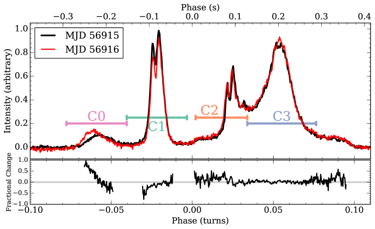
Figure 1: Upper Panel: Mean profiles of J1745$-$2900 observed on two consecutive days (MJD 56915, 56916). The profiles have been normalized so that the area under each is the same. The horizontal bars give the name and range of the four profile components. Lower Panel: The fractional difference between the two profiles.

While the mean profiles appear consistent over 1 day, this is not the case on longer time-scales. Figure 2 shows a collection of J1745$-$2900 profiles generated from phased-array VLA data spanning ${\sim}600$ days. In addition to one of our profiles (MJD 56915), there are six profiles obtained commensally during VLBI observations of J1745$-$2900 using the phased VLA at 8.7 GHz with 256 MHz of bandwidth (Bower et al. 2014, 2015). Since no phase-connected timing solution exists over this interval (Kaspi et al. 2014; Lynch et al. 2015), we have simply aligned the profiles by the rightmost peak (our C3).

From Figure 2, it is clear that J1745$-$2900 undergoes significant profile changes on long time scales. This behavior is consistent with the results from other monitoring campaigns. Lynch et al. (2015) observed J1745$-$2900 with the GBT at 8.5 GHz once per week over the 167 days from MJD 56515–56682 and once per two weeks over the 130 days from MJD 56726–56856. During the earlier period (MJD 56515–56682), they found only minor changes to the mean profile as two components gradually separate. In the later period (MJD 56726–56856) the mean profile changes considerably, with components appearing and disappearing. Based on our VLA observations, it is likely that the period of gradual change extended at least until MJD 56710 (28 days beyond the last weekly GBT observation). Significant profile changes are also seen by Yan et al. (2015) in six 8.6 GHz observations with the Tian Ma Radio Telescope (TMRT) over the 107 day span from MJD 56836–56943. Two of these observations occurred on consecutive days (MJD 56911, 56912) a few days before our observations. These profiles are similar both to each other and to the profiles we observe on MJD 56915-6, although the much lower sensitivity prevents a more robust comparison. Profile stability on day time-scales is consistent with our observations (Figure 1). Profile changes are also seen at frequencies of $89-291$ GHz (Torne et al. 2015, 2017), which strongly suggests a magnetospheric origin for these changes.

Figure 2: Folded pulse profiles of J1745$-$2900 from phased-array VLA observations. The profile for MJD 56915 comes from a 6.5 hour observation using 4 GHz of bandwidth. The remaining profiles are from a VLBI campaign that used the phased VLA at 8.7 GHz using 256 MHz of bandwidth and observing times of about six hours (Bower et al. 2015). The pulse profiles have been aligned so that the rightmost peak (our C3) of each pulse is roughly aligned.

3.2 Frequency Evolution

Many pulsars show a gradual change in profile shape as a function of observing radio frequency (Thorsett 1991; Chen & Wang 2014). We can test whether there is a similar effect in our J1745$-$2900 data by splitting the 4 GHz bandwidth into four 1 GHz sub-bands (B0, B1, B2, B3) and generating mean profiles for each band. The resulting profiles for the MJD 56915 data set are shown in Figure 3 along with the fractional difference between the profile generated from the highest frequency sub-band and the other three sub-bands.

From Figure 3, we see that the mean profile of J1745$-$2900 is essentially consistent from 7.7–11.6 GHz, with a few slight changes. For one, each of the peaks in the components C1, C2, and C3 narrow with increasing frequency. Another slight change is that the height of the bridge from C2 to C3 appears to be increasing with frequency, although this may be an artifact of the normalization of the pulses to equal area. Finally, it seems as though the amplitude of C1 decreases with increasing frequency.

The modest profile evolution in frequency seen here in J1745$-$2900 is consistent with that seen in radio pulsars at comparable frequencies (Kramer et al. 1997; Johnston et al. 2008). In general, though, radio-emitting magnetars seem to show more complex behavior. Kramer et al. (1997) conducted a multifrequency study of XTE J1810$-$197 and found that the average profile could change significantly (e.g., appearance or disappearance of components) from $1.4-8.4~{}\rm GHz$. Previous studies of J1745$-$2900 have also shown significant profile changes from $2.5-8.4~{}\rm GHz$ in some epochs (Torne et al. 2015) and almost no frequency evolution in others (Torne et al. 2017). This suggests that the frequency evolution of the average profile of J1745$-$2900 is time-dependent.

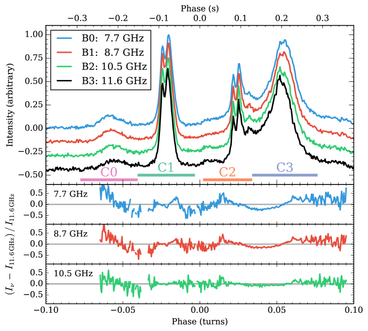
Figure 3: Frequency evolution of J1745$-$2900 pulse profile for MJD 56915. Upper Panel: Mean profiles generated using 1 GHz sub-bands (lowest frequency on top, highest on bottom). The center frequency of each sub-band is shown in the legend. The profiles have been normalized so that the area under each pulse is the same. Horizontal bars indicate the range of the profile components. Lower Panels: Fractional difference between each of the three lower sub-bands and the sub-band centered on 11.6 GHz.

4 Single Pulse Properties

In each of our observations, we have collected single pulse data from nearly 5000 rotations of J1745$-$2900. Owing to the brightness of the magnetar and the sensitivity of the VLA, individual sub-pulses are clearly seen in almost every rotation. Figure 4 shows a selection of 900 rotations ($\approx 3400$ s) of the magnetar from MJD 56915. The wide ($\approx 700$ ms) mean profile is comprised of much narrower ($\sim 1-10$ ms) single pulses that appear to show a large degree of rotational phase jitter. As such, this is an excellent data set to quantify the jitter and to search for any correlations in the properties of sub-pulses occurring in each of the profile components. Because the MJD 56916 observation contained a significant amount of RFI, we only use single pulses from MJD 56915 in this analysis.

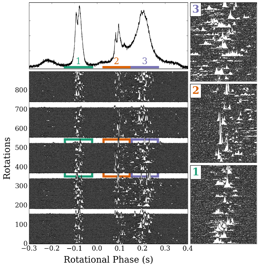
Figure 4: Stacked single pulses from 900 rotations ($\approx 3400$ s) of J1745$-$2900 from MJD 56915. The 100 s ($\approx 27$ rotations) calibrator scans are seen as gaps in between the 600 s ($\approx 160$ rotations) on source scans. The upper panel shows the mean profile from the full observation. Panels on the right give a zoomed in view of the pulses showing 120 ms of rotational phase over one 600 s on source scan.

4.1 Single Pulse Characterization

To quantify the single pulse behavior of J1745$-$2900, we determine the amplitude, arrival time, and width of the pulse in each profile component for every rotation of the magnetar. We use a matched filter technique from pulsar timing in which the intensity, $I(t)$, of a pulse is represented as a scaled and shifted template, $G(t)$, in the presence of noise so that

$$I(t)=b\,G(t-\tau)+c+n(t)$$ (1)

where $b$ and $c$ are constants and $n(t)$ is noise. The scale ($b$) and shift ($\tau$) parameters are found through fitting in the Fourier domain (Taylor 1992). We use a Python implementation of this fitting technique from the PyPulse software package (Lam 2017).

In pulsar timing, the template is typically taken to be the mean profile. The mean profile of J1745$-$2900 is far too wide to be useful for fitting the narrow pulses in each profile component, so we instead use Gaussians. Since the pulses appear to have a range of widths, we draw from a template bank of Gaussian functions with full-width at half-maximum (FWHM) values of $w=2^{m}\delta t$ for $m\in[1,8]$ samples, which is $0.2-51.2~{}\rm ms$ for our time resolution of $\delta t=0.2~{}\rm ms$. The width of the pulse corresponds to the width of the template that maximizes signal to noise ratio. This is done for each profile component. Thus, our fitting procedure returns an estimate for the amplitude ($\hat{b}$ in units of the noise standard deviation), time-of-arrival offset ($\hat{\tau}$), and width ($\hat{w}$) of a pulse within each profile component for each rotation of the magnetar.

4.2 Pulse Width Distribution

It is clear from Figure 4 that individual pulses are seen with a variety of widths. Using the measured widths from the template fitting, we determine the pulse width distribution for pulses from each profile component. Figure 5 shows the width distribution for pulses with $\hat{b}>5$ (that is, $\rm S/N>5$). The most common pulse width for all components is either 3.2 or 6.4 ms. There are no pulses found with the narrowest template ($\rm FWHM=0.2~{}\rm ms$) and only in component C3 are there pulses found with the widest template ($\rm FWHM=51.2~{}\rm ms$). As seen in Figure 4, these wide pulses are often comprised of many narrower (possibly overlapping) sub-pulses.

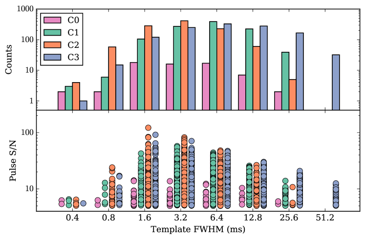
Figure 5: Distribution of pulse widths for pulses in each of the four profile components with a threshold of ${\rm S/N}>5$. Upper Panel: Histogram of pulse widths for each component. The total number of pulses in component (C0, C1, C2, C3) is (64, 1038, 1053, 1191). Lower Panel: The $\rm S/N$ for each above-threshold pulse as a function of width.

4.3 Pulse Jitter

Even though the mean profile of most pulsars is stable, the pulses from individual rotations can vary in both shape and arrival phase. This phenomenon is called pulse jitter and is clearly present in the single pulses shown in Figure 4. Following similar analyses in pulsar timing, we can estimate the contribution of pulse jitter to the overall time-of-arrival (TOA) measurement error. Unlike most pulsar timing experiments, we will consider pulses from each profile component separately. The TOA measurement error, $\sigma_{\rm TOA}$, can be expressed as

$$\sigma^{2}_{\rm TOA}=\sigma^{2}_{\rm S/N}+\sigma^{2}_{\rm DISS}+\sigma^{2}_{\rm J}$$ (2)

where $\sigma_{\rm S/N}$ is the template fitting error, $\sigma_{\rm DISS}$ is the contribution to the uncertainty caused by diffractive interstellar scintillation (DISS), and $\sigma_{\rm J}$ is the pulse jitter (Cordes & Shannon 2010). By measuring or estimating $\sigma_{\rm TOA}$, $\sigma_{\rm S/N}$, and $\sigma_{\rm DISS}$, we can determine $\sigma_{\rm J}$.

The template fitting error, $\sigma_{\rm S/N}$, quantifies the contribution of purely additive noise to the timing error. It depends on the pulse signal to noise ratio (S/N), so will vary from pulse to pulse, but for our data set we see typically see $\sigma_{\rm S/N}\lesssim 0.1~{}\rm ms$. Since we use a simple Gaussian template, there may also be some additional error caused by the slight differences between the template and the intrinsic pulse shape. Based on the distribution of pulse widths (Figure 5), we do not expect this to be more than $\sim 1~{}{\rm ms}$.

The DISS term is the result of averaging each pulse over a finite number of scintles in the time-frequency plane and can be estimated as $\sigma_{\rm DISS}\approx\tau_{\rm d}/\sqrt{N_{\rm s}}$, where $\tau_{\rm d}$ is the scattering time and $N_{\rm s}$ is the number of scintles. The number of scintles is given by

$$N_{\rm s}\approx\left(1+\eta\frac{B}{\Delta\nu_{\rm d}}\right)\left(1+\eta\frac{T}{\Delta t_{\rm d}}\right)$$ (3)

where $\eta$ is the scintle filling factor, $B$ is the bandwidth, $T$ is the integration time, $\Delta t_{\rm d}$ is the diffractive time-scale, and $\Delta\nu_{\rm d}$ is the diffractive bandwidth (Cordes & Lazio 1991). The diffractive bandwidth is related to the scattering time as $\Delta\nu_{\rm d}=1.16/(2\pi\tau_{\rm d})$ (Cordes & Rickett 1998). Using a 10 GHz scattering time of $\tau_{\rm d}=0.1~{}\rm ms$ (Section 5), we expect $\Delta\nu_{\rm d}\approx 1800~{}{\rm Hz}~{}(\tau_{\rm d}/0.1~{}\rm ms)^{-1}$. The diffractive time-scale for a single thin scattering screen is $\Delta t_{\rm d}=\ell_{\rm d}/v=\lambda/(2\pi\theta_{\rm d}v)\sim 1~{}\rm s$, where $\lambda=3.5~{}\rm cm$, $\theta_{\rm d}=15~{}\rm mas$, and $v\sim 100~{}\rm{km~{}s}^{-1}$ (Bower et al. 2015). Taking $\eta\approx 0.3$, $T=3.76~{}\rm s$, and $B=4~{}\rm GHz$, we find that the DISS contribution to the TOA uncertainty is only $\sigma_{\rm DISS}\approx 0.1~{}\mu\rm s$.

The single pulse TOA measurement error, $\sigma_{\rm TOA}$, is simply the observed scatter in TOA offsets ($\hat{\tau}$) measured for the pulses in each profile component. It varies between the components, but typical values are $\sigma_{\rm TOA}\gtrsim 20~{}\rm ms$. Since $\sigma_{\rm TOA}\gg\sigma_{\rm S/N}\gg\sigma_{\rm DISS}$, the single pulse TOA measurement error in every component is entirely dominated by the jitter so $\sigma_{\rm J}\approx\sigma_{\rm TOA}$.

The pulse phase jitter is correlated over typical observing bands, but can decorrelate over larger bandwidths. In a study of millisecond pulsars, Shannon et al. (2014) found that the jitter in PSR J0437$-$4715 decorrelates between 0.75$-$3.1 GHz, giving a jitter correlation bandwidth of $\lesssim\!2$ GHz. To test the jitter correlation bandwidth of J1745$-$2900, we split the full 4 GHz band into four 1 GHz sub-bands (centered on frequencies of 7.7, 8.7, 10.5, and 11.6 GHz), characterize the pulses in each component for each sub-band, and then compare the results. Instead of searching over a range of pulse widths, we just use a single template with $\rm FWHM=10~{}ms$ (50 time samples). This ensures a consistent comparison of pulses in different frequency bands. Figure 6 shows the TOA offsets measured in component C1 for all the sub-bands plotted against each other. Plots from other profile components are similar. The pulse phase jitter in J1745$-$2900 is highly correlated over 4 GHz of bandwidth.

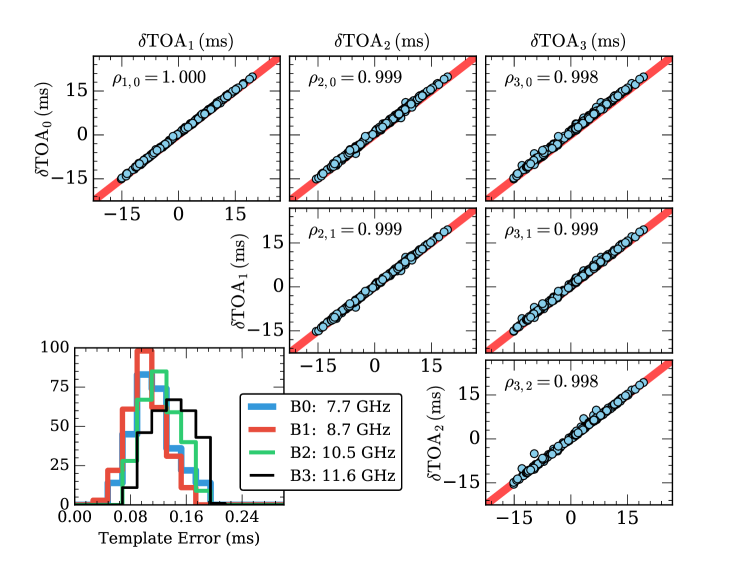
Figure 6: Comparison of time-of-arrival (TOA) offsets for single pulses from profile component C1 measured in four 1 GHz sub-bands. We selected the 288 pulses detected with $\rm S/N>5$ in all four bands and calculated the TOA offsets using a Gaussian template with a full-width at half-max of 10 ms. The correlation coefficient for each pairwise comparison of sub-bands is shown in each panel. The lower left panel shows the distribution of template fitting errors, $\sigma_{\rm S/N}$, for all the pulses.

4.4 Correlations between Profile Components

In Section 4.3, we showed that the TOA measurement error of pulses within each profile component is dominated by jitter. Here we explore whether there are any correlations between the TOA offsets or amplitudes of these pulses. Any correlation in the properties of pulses between components could indicate a common origin for pulsed emission.

To look for correlations, we first generate time series data for the pulse properties of interest from each profile component using the methods described in Section 4.1 and a threshold of $\rm(S/N)_{\rm min}=5$. We determine the TOA offset ($\hat{\tau}[n]$), the pulse amplitude ($\hat{b}[n]$), and a binary value ($\Theta[n]$) indicating the presence of an above threshold pulse all as a function of the pulse number ($n$). Next, the cross-correlation function (CCF) is calculated between the time series of two profile components for each pulse parameter of interest. We denote the CCF as

$${\rm CCF}_{ij}(x)[n]=\left(x_{i}\star x_{j}\right)[n]$$ (4)

where $x$ is the time series parameter ($\hat{b},\hat{\tau},\Theta$) from the profile components $i,j\in\{\rm C0,C1,C2,C3\}$ normalized to have zero mean and unit variance. To avoid the periodicity introduced by the calibrator scans, the CCFs are calculated using data from each on-source scan and then averaged together over all scans.

To determine the significance of any CCF peaks, we shuffle all the values in the time series of each parameter and re-calculate the CCF, repeating this process $10^{4}$ times. Since the shuffled time series should have no correlations, we can use these results to set the 99.7% ($\approx 3\sigma$) confidence level for any lag value in the CCFs.

The results of this analysis are shown in Figure 7. We calculate ${\rm CCF}_{ij}(x)[n]$ for each parameter ($\hat{b},\hat{\tau},\Theta$) for component pairs $(i,j)=\rm(C1,C2)$, $\rm(C1,C3)$, and $\rm(C2,C3)$. Component C0 was excluded because it had far fewer above threshold pulses ($N=64$) than C1 ($N=1038$), C2 ($N=1053$), and C3 ($N=1191$). While most of the CCFs appear to be consistent with noise, there is a small but significant correlation in the occurrence of pulses in C1 and C2 at zero lag. This means that pulses in C1 and C2 occur during the same rotation of J1745$-$2900 more often than would be expected if they were completely independent.

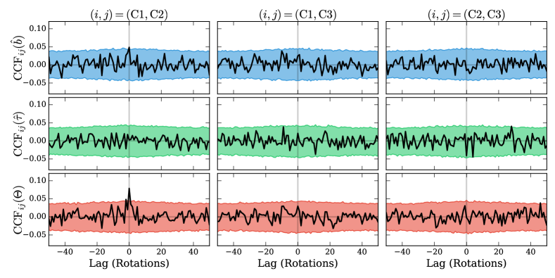
Figure 7: Cross-correlation function (CCF) between the time series of pulse properties measured in the three brightest pulse profile components. The black lines denote the observed CCF and the light shaded regions denote the 99.7% ($\approx 3\sigma$) confidence limit estimated by reshuffling the pulse order (see text for details). Upper Row: CCF of observed pulse amplitudes ($\hat{b}$). Middle Row: CCF of observed pulse TOA offsets ($\hat{\tau}$). Lower Row: CCF of above threshold pulse occurrence ($\Theta$).

5 Dispersion and Scattering in Single Pulses

As a bright radio-emitting magnetar in the immediate vicinity of Sgr A*, J1745$-$2900 is an excellent tool for studying the magneto-ionic environment along the line of sight to the Galactic center. Measurements of the dispersion measure and scattering time are easiest for bright and narrow pulse profiles. The broad jitter-dominated average profile of J1745$-$2900 is not well suited for these measurements at 10 GHz, but some of the individual sub-pulses are. Here we use a set of bright narrow sub-pulses (hereafter just referred to as pulses) to measure the dispersion and scattering parameters for J1745$-$2900.

5.1 Pulse Selection

To get the best measurements of the dispersion measure and pulse broadening time, we need to select pulses that have high S/N and small widths. Using the pulse parameters determined in Section 4.1, we select pulses with $\rm S/N>30$ and $\hat{w}\leq\rm 8~{}bins=1.6~{}\rm ms$. A total of 40 pulses meet these criteria, but two are excluded (one for missing data and one for having a wide and complicated pulse structure). Of the 38 remaining pulses, none are from component C0, 2 are from C1, 23 are from C2, and 13 are from C3. Only one of the selected pulses has a width of $\hat{w}=4~{}\rm bins$ (0.8 ms), the rest have a width of $\hat{w}=8~{}\rm bins$ (1.6 ms). The widths are only approximate, though, as they were found by matched filtering using Gaussian templates. The actual pulses can show more complicated structure than the templates. Figure 8 shows the frequency-resolved and frequency-summed profiles for six of the 38 pulses.

5.2 Method

Using the sample of 38 bright and narrow pulses, we can measure the dispersion and scattering by modeling the frequency-dependent delay across the observing band. Dispersion introduces a delay in the arrival time of a pulse that scales as $\tau_{\rm DM}\propto\nu^{-2}$. Multipath scattering distorts the pulse so that the observed pulse shape is the intrinsic pulse shape convolved with a one-sided exponential with time-scale $\tau_{\rm sc}\propto\nu^{\alpha_{\rm sc}}$. This asymmetric distortion produces a frequency-dependent shift in the observed arrival time of a pulse. When the scattering time is small compared to the pulse width, the frequency-dependent shift in the measured arrival time of a pulse can be approximated as

$$\tau(\nu)=k_{\rm DM}{\rm DM}\,\left(\frac{\nu}{1~{}{\rm GHz}}\right)^{-2}+\tau_{\rm sc,10}\left(\frac{\nu}{10~{}{\rm GHz}}\right)^{\alpha_{\rm sc}}+t_{0}$$ (5)

where $k_{\rm DM}=4.15~{}\rm ms~{}GHz^{2}~{}pc^{-1}~{}cm^{3}$ is the dispersive constant, ${\rm DM}$ is the dispersion measure, $\tau_{\rm sc,10}$ is the scattering time at $10~{}\rm GHz$, $\alpha_{\rm sc}$ is the scaling index of the scattering law, and $t_{0}$ is an offset. The scattering index is fixed at $\alpha_{\rm sc}=-4.0$, which is consistent with the $\alpha=-3.8\pm 0.2$ measured for J1745$-$2900 by Spitler et al. (2014). We have found that the approximation of Equation 5 is accurate to about 10% for scattering times less than about 20% the width of a pulse.

Using the channelized time series data, sub-band arrival times for each pulse can be determined using the same matched filter method used in Section 4.1. For each pulse, we average together several frequency channels to ensure that $\rm S/N>5$ detections can be made in each sub-band. Of the 38 pulses in our sample, (10, 16, 11, 1) pulses use sub-band bandwidths of (32, 64, 128, 256) MHz. Using the measured arrival times and arrival time uncertainties in each sub-band, we fit for the parameters of the delay model (Equation 5) for each pulse separately and for all pulses jointly.

Assuming normally distributed errors in the measured sub-band arrival times, the likelihood function for a single pulse fit is

$$\mathcal{L}(\tau|{\rm DM},\tau_{\rm sc,10},t_{0})=\prod_{i=0}^{N-1}\frac{1}{\sqrt{2\pi\sigma_{\tau,i}^{2}}}\exp\left[-\frac{1}{2}\left(\frac{\tau_{i}-\tau(\nu_{i})}{\sigma_{\tau,i}}\right)^{2}\right]$$ (6)

where $\tau_{i}$ and $\sigma_{\tau,i}$ are the arrival time and arrival time uncertainty in the sub-band with center frequency $\nu_{i}$. Wide priors are adopted for each of the parameters. Normal distributions are used for the priors of $\rm DM$ ($\mu_{\rm DM}=2000~{}{\rm pc~{}cm}^{-3}$, $\sigma_{\rm DM}=1000~{}{\rm pc~{}cm}^{-3}$) and $t_{0}$ ($\mu_{t}=0~{}{\rm ms}$, $\sigma_{t}=500~{}{\rm ms}$). For the 10 GHz scattering time $\tau_{\rm sc,10}$, an exponential distribution with mean $\lambda_{\tau}=2~{}\rm ms$ is used as a prior. Combining these priors with the likelihood, we can construct and sample the posterior distribution using the emcee MCMC sampler (Foreman-Mackey et al. 2013). In addition to fitting each pulse separately for ($\rm DM$, $\tau_{\rm sc,10}$, $t_{0}$), we can also do a global fit that assumes one set of ($\rm DM$, $\tau_{\rm sc,10}$) for all pulses.

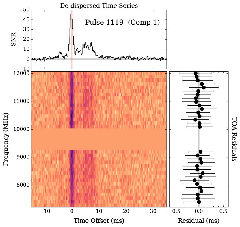
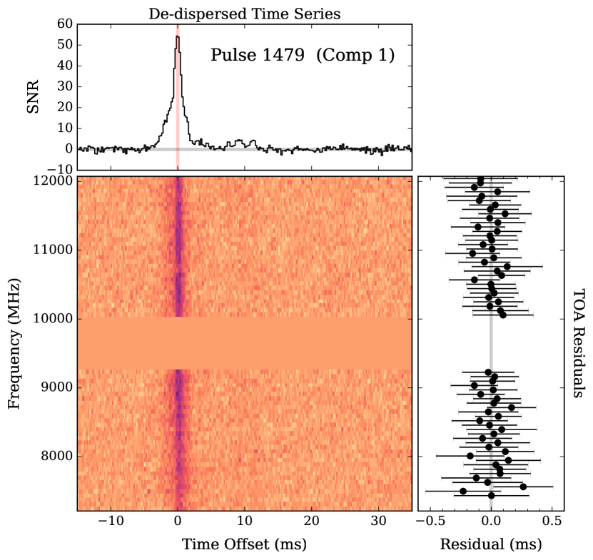
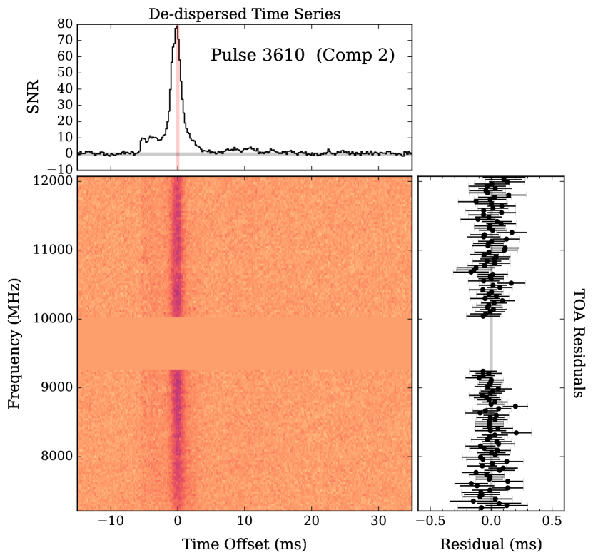
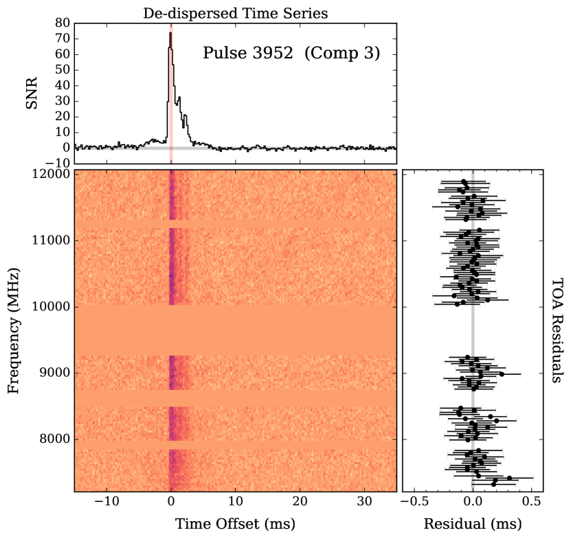
Figure 8: A sample of six of the 38 pulses used to fit for the dispersion measure and scattering. Each panel shows the dispersion corrected frequency-resolved pulse (middle), the de-dispersed time series (top), and residual delays after subtracting the global best-fit model (right). The frequency range from 9.2–10 GHz was avoided due to strong RFI and other gaps are the result of RFI masking.

5.3 Results

The global fit for all 38 pulses gives $\rm DM=1760.0^{+2.4}_{-1.3}~{}{\rm pc~{}cm}^{-3}$ and $\tau_{\rm sc,10}=0.09\pm 0.03~{}\rm ms$. Figure 9 shows the joint posterior distribution $p(\rm DM,\tau_{\rm sc,10})$ marginalized over all $\{t_{0,i}\}$ and the fully marginalized posteriors $p({\rm DM})$ and $p(\tau_{\rm sc,10})$. The best fit values and uncertainties for $\rm DM$ and $\tau_{\rm sc,10}$ are taken as the maximum and most compact inner 68% of the fully marginalized posteriors for each parameter.

Figure 10 shows the individual fits of $\rm DM$ and $\tau_{\rm sc,10}$ for each of the 38 pulses. The best fit values and uncertainties of $\rm DM$ and $\tau_{\rm sc,10}$ for each pulse are taken as the maximum and most compact inner 68% of the fully marginalized posteriors for each parameter. All of the individual pulse fits are consistent with constant values for $\rm DM$ and $\tau_{\rm sc,10}$ over the course of the 6 hour observation.

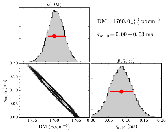
Figure 9: Marginalized posterior distributions for the global fit using 38 single pulses. The two dimensional distribution in the lower left gives the joint posterior distribution of $\rm DM$ and $\tau_{\rm sc,10}$ marginalized over all 38 offset terms $\{t_{0,i}\}$. The grey histograms give the fully marginalized posterior distributions for the $\rm DM$ (top left) and $\tau_{\rm sc,10}$ (bottom right). The peak value and compact innermost 68% of the posteriors for each parameter are indicated by the red marker and bar.

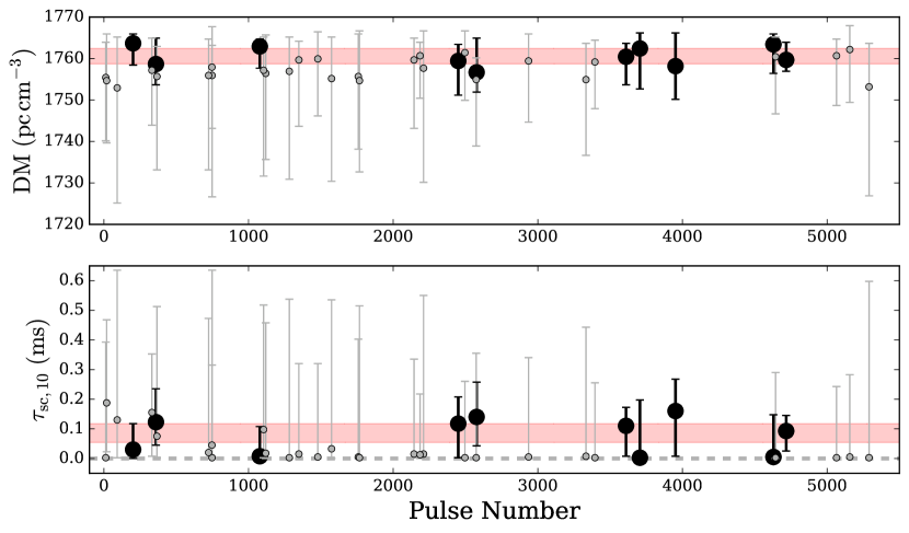
Figure 10: Individual fits for the dispersion measure (top) and 10 GHz scattering time (bottom) for each of the 38 pulses used in the global fit. The points give the maximum of the fully marginalized posterior for each parameter and the errorbars denote the innermost compact 68% region. For clarity, the parameter values for pulses with the most constraining individual fits ($\rm\delta DM<10~{}{\rm pc~{}cm}^{-3}$) are shown with large black markers. Parameters from other pulses are shown as smaller grey markers. The red bands give the global fit measurements of $\rm DM=1760.0^{+2.4}_{-1.3}~{}{\rm pc~{}cm}^{-3}$ and $\rm\tau_{\rm sc,10}=0.09\pm 0.03~{}ms$.

5.4 Comparison with Previous Results

Shortly after the discovery of radio pulsations from J1745$-$2900, several measurements of the dispersion and scattering were made. Eatough et al. (2013) measured the dispersion measure of J1745$-$2900 to be $\rm DM=1778\pm 3~{}{\rm pc~{}cm}^{-3}$ from pulsar timing observations over a frequency range of 2.5–8.5 GHz. Spitler et al. (2014) conducted a multifrequency study of J1745$-$2900 using multiple telescopes to measure the parameters of the scattering law. They found a 1 GHz scattering time of $\tau_{\rm sc,1}=1300\pm 200~{}\rm ms$ and a scattering index of $\alpha_{\rm sc}=-3.8\pm 0.2$. Pennucci et al. (2015) observed J1745$-$2900 with the GBT in two observing bands to cover 1.4–2.4 GHz and used a wide-band model to simultaneously fit the scattering and dispersion parameters. Over 28 days of observing, they measured values ranging from $\rm DM\approx 1770-1800~{}{\rm pc~{}cm}^{-3}$ and showing an apparent variability in both time and frequency. More recently, Desvignes et al. (2018) presented the results of the long-term monitoring campaign of J1745$-$2900 that began with the Eatough et al. (2013) observations. Observing over the frequency range of 2.5–8.5 GHz over a four year span, they found that the dispersion measure was consistent (at the $2\sigma$ level) with a constant value of $\rm DM=1762\pm 11~{}{\rm pc~{}cm}^{-3}$. Finally, Pearlman et al. (2018) reported a large ($\tau_{\rm sc,8.4}\approx 6~{}\rm ms$) and variable scattering time at 8.4 GHz with the Deep Space Network 70-m telescope DSS-43.

Our measurement of a 10 GHz pulse broadening time of $\tau_{\rm sc,10}=0.09\pm 0.03~{}\rm ms$ is consistent with the $\tau_{\rm sc,10}=0.1-0.3~{}\rm ms$ expected at 10 GHz from the Spitler et al. (2014) scattering relation, but is much less than the $\tau_{\rm sc,10}\approx 3~{}\rm ms$ expected from the Pearlman et al. (2018) result. Our DM measurement of $\rm DM=1760.0^{+2.4}_{-1.3}~{}{\rm pc~{}cm}^{-3}$ is consistent with the $\rm DM=1762\pm 11~{}{\rm pc~{}cm}^{-3}$ value seen by Desvignes et al. (2018) over a four year span. However, both our value and that of Desvignes et al. (2018) are $\Delta\rm DM\approx 10-40~{}{\rm pc~{}cm}^{-3}$ smaller than the early measurements by Eatough et al. (2013) and Pennucci et al. (2015). The discrepancies in DM and scattering time are discussed in Section 6.3.

6 Discussion

We have conducted a detailed study of single pulses from the radio-emitting magnetar J1745$-$2900 using the VLA in its phased-array pulsar mode at 7–12 GHz.

6.1 Profile Evolution

We have studied both the time and frequency evolution of the average profile of J1745$-$2900. Using two 6.5 hour observations on consecutive days, we found that the average pulse profile was stable on $\sim$day timescales. Comparison with additional phased VLA observations at 8.7 GHz from July 2013 to February 2015, shows that the average pulse profile of J1745$-$2900 changes on longer timescales. This profile variability is consistent with previous observations of J1745$-$2900 over a range of frequencies (Lynch et al. 2015; Yan et al. 2015, 2018; Torne et al. 2015, 2017) and with studies of other radio-emitting magnetars (Camilo et al. 2007a), which suggests a magnetospheric origin.

Using 5 GHz of simultaneous bandwidth from a single epoch, we also found that the profile is fairly stable over a frequency range of 7–12 GHz ($\Delta\nu/\nu\approx 0.5$), showing only a slight narrowing of components with increasing frequency. This modest evolution is consistent with what is seen in radio pulsars at comparable frequencies (Kramer et al. 1997; Johnston et al. 2008). Radio-emitting magnetars (including J1745$-$2900) have shown large profile changes (e.g., the appearance and disappearance of components) over frequency ranges of $\sim\!\rm GHz$ (Kramer et al. 2007; Torne et al. 2015). However, J1745$-$2900 has also been observed with a stable pulse profile from $2-8~{}\rm GHz$ (Torne et al. 2017), so the frequency evolution may also be time-dependent.

6.2 Single Pulses

The wide ($\approx 700$ ms) profile of J1745$-$2900 in our observations is comprised of much narrower ($\sim 1-10$ ms) single pulses. This spiky pulse emission is uncommon in radio pulsars, but appears to be characteristic of radio-emitting magnetars (Kramer et al. 2007; Levin et al. 2012). To study these pulses, we used a matched-filter technique to characterize the pulses in each profile component for every available rotation of J1745$-$2900 in our data. Comparing the occurrence, amplitude, and arrival time of pulses in each profile component, we find no correlation in the amplitude or phase of pulses occurring in different profile components. However, we do find a statistically significant over-abundance of pulses occurring during the same rotation in both components C1 and C2, possibly suggesting a common or related origin for pulses in these two profile components. We also measured the frequency correlation of the single pulse jitter of sub-pulses in each of the four profile components. Using data from four 1 GHz sub-bands, we found that the jitter is $\approx 100\%$ correlated over the full $7-12$ GHz VLA band.

6.3 Dispersion Measure and Scattering

Variations in the dispersion measure and scattering time of J1745$-$2900 probe the inhomogeneities of the distribution of free electrons along the line of sight to the Galactic center. Measuring the magnitude and timescale of these variations can help disentangle the contributions to the DM and scattering within the Galactic center from those occurring along the line of sight in the Galactic plane. Any significant variation in the scattering time would also have important implications for strategies to find pulsars near Sgr A*. Our single epoch (MJD 56915) measurement of the DM and scattering time cannot say much about variability itself, but is useful in the context of other published measurements.

6.3.1 Scattering Variations

Our measurement of the 10 GHz scattering time on MJD 56915 is consistent with the values measured by Spitler et al. (2014) from MJD 56418-98, but this does not rule out the possibility that the scattering time is variable. The relatively large uncertainty in our measurement is such that it may differ from the Spitler et al. (2014) relation by a factor of a few. Furthermore, it could be the case that scattering is sporadically enhanced due to small scale features in the Galactic center. Future attempts to measure the scattering in single pulses should note the intrinsic asymmetry in some of the pulses we have observed (Figure 8). Had we ignored the frequency dependence of the scattering time and just fit a Gaussian convolved with an exponential, we would have mistaken this intrinsic structure for scattering times as high as several milliseconds.

6.3.2 DM Variations

Desvignes et al. (2018) presented the DM of J1745$-$2900 for over 1500 days (starting soon after the detection of radio pulsations), with measurements at 2.5, 4.85, and 4-8 GHz. Our measurement of $\rm DM=1760.0^{+2.4}_{-1.3}~{}{\rm pc~{}cm}^{-3}$ on MJD 56915 is consistent with the most precise single epoch measurement reported by Desvignes et al. (2018) of $\rm DM=1765\pm 4~{}{\rm pc~{}cm}^{-3}$ 898 days later (MJD 57813). All of the high frequency (4.85, 4-8 GHz) DM measurements from Desvignes et al. (2018) also appear consistent with a constant value of ${\rm DM}\approx 1760~{}{\rm pc~{}cm}^{-3}$, although most of the measurements have uncertainties of $\sigma_{\rm DM}\approx 15-25~{}{\rm pc~{}cm}^{-3}$ so variations below this level cannot be excluded.

Our DM measurement is $\Delta\rm DM\approx 10-40~{}{\rm pc~{}cm}^{-3}$ smaller than lower frequency ($\nu\approx 1-2~{}\rm GHz$) measurements in the first $\approx\!\!400$ days afer radio pulsations were detected from J1745$-$2900. Eatough et al. (2013) used pulsar timing observations at 2.5 and 8.5 GHz and found $\rm DM=1778\pm 3~{}{\rm pc~{}cm}^{-3}$ shortly after the first detection of radio pulsations (MJD 56414). Pennucci et al. (2015) found a range of $\rm DM\approx 1770-1800~{}{\rm pc~{}cm}^{-3}$ using the GBT in two observing bands to cover 1.4–2.4 GHz over a 28 day span from MJD 56488-516. The 2.5 GHz DM measurements from Desvignes et al. (2018) over the first $\approx\!\!400$ days after the magnetar radio detection also appear to be systematically higher, though the uncertainties are large.

There are a few possible explanations for the discrepancy between our DM and the early low-frequency measurements. One possibility is that the DM decreased by $\Delta\rm DM\approx 10-40~{}{\rm pc~{}cm}^{-3}$ over the $\approx\!\!400$ days between the radio detection and our measurements. Such a change could occur if the magnetar travels far enough through the dense ionized gas found in the Galactic center. Taking a line of sight velocity to be comparable to the transverse velocity of $v_{\perp}=236\pm 11~{}{\rm km~{}s}^{-1}$ measured by Bower et al. (2015), J1745$-$2900 travels a distance of

$$\Delta L\approx 2\times 10^{-4}~{}{\rm pc}~{}\left(\frac{v_{\rm los}}{200~{}{\rm km~{}s}^{-1}}\right)\left(\frac{t}{400~{}{\rm days}}\right)$$ (7)

in the 400 days between $\rm DM$ measurements. In order to fully explain the difference in $\rm DM$, the mean electron density needs to be $\bar{n}_{\rm e}=\Delta{\rm DM}/\Delta L\approx 10^{5}~{}{\rm cm}^{-3}$. This value is just within the range of electron densities ($n_{\rm e}\approx 0.2-1\times 10^{5}~{}{\rm cm}^{-3}$) estimated along Sgr A West towards J1745$-$2900 by Zhao et al. (2010) based on radio recombination line measurements. However, Sgr A West has an estimated depth of $d_{\rm W}\sim 0.1~{}\rm pc$ (Ferrière 2012). For the contribution to the observed $\rm DM$ to be $\rm DM_{w}\lesssim 100~{}{\rm pc~{}cm}^{-3}$ (for consistency with other Galactic center pulsars), J1745$-$2900 could only be $d\lesssim 0.001~{}\rm pc$ within Sgr A West. Outside Sgr A West, the typical electron density of the warm ionized gas in the central cavity is $n_{\rm e,c}\sim 10^{3}~{}{\rm cm}^{-3}$ (Ferrière 2012), which would only produce $\Delta\rm DM\approx 0.2~{}{\rm pc~{}cm}^{-3}$. For the observed $\Delta\rm DM$ to be real, then, J1745$-$2900 would need to be located just barely within the densest parts of Sgr A West. While not impossible, this seems unlikely.

Another possibility is that the measured DM depends on the observing frequency. Cordes et al. (2016) describe how frequency dependent DMs can arise from multipath propagation in the turbulent ISM. Basically, the measured DM at a given observing frequency is the average of many paths that pass through the scattering disk. Since the scattering disk is frequency-dependent ($\theta_{\rm sc}\propto\nu^{-2}$), different observing frequencies will sample different paths through the ISM. However, the predicted offsets between DMs measured at 2 GHz and 4, 6, or 10 GHz are only $\delta{\rm DM}\sim 1~{}{\rm pc~{}cm}^{-3}$, so this effect is likely insufficient to make up the difference.

The final possibility is that the difference is the result of systematic biases in the different methods for measuring the DM and scattering. We have used a collection of bright and narrow single pulses to make our measurements, but the earlier lower frequency measurements all used integrated profiles. As shown in Figure 2, the average profiles can have widths of $W_{\rm avg}\gtrsim 100~{}{\rm ms}$ and sometimes show multiple (possibly overlapping) profile components. Depending on the method used, this could potentially affect the DM and scattering measurements. For example, fitting a single Gaussian convolved with an exponential scattering tail to an overlapping double peaked profile could result in a measured DM that is incorrect. By instead measuring the time delays of narrow single pulses, we should have avoided these issues. By jointly fitting many pulses, we further reduce the effect of individual pulse shapes. While single pulse fitting may have its own biases, they are likely different than those encountered in the average profile fitting. We consider this the most likely explanation for the difference in observed DMs, but a long-term campaign to measure both DM and scattering at lower frequencies is likely needed to resolve this issue.

References

- Bower et al. (2014) Bower, G. C., Deller, A., Demorest, P., Brunthaler, A., et al. 2014, ApJ, 780, L2
- Bower et al. (2015) Bower, G. C., Deller, A., Demorest, P., et al. 2015, ApJ, 798, 120
- Camilo et al. (2007a) Camilo, F., Cognard, I., Ransom, S. M., et al. 2007a, ApJ, 663, 497
- Camilo et al. (2007b) Camilo, F., Ransom, S. M., Halpern, J. P., & Reynolds, J. 2007b, ApJ, 666, L93
- Camilo et al. (2006) Camilo, F., Ransom, S. M., Halpern, J. P., Reynolds, J., et al. 2006, Nature, 442, 892
- Chen & Wang (2014) Chen, J. L., & Wang, H. G. 2014, ApJS, 215, 11
- Cordes & Lazio (1991) Cordes, J. M., & Lazio, T. J. 1991, ApJ, 376, 123
- Cordes & Rickett (1998) Cordes, J. M., & Rickett, B. J. 1998, ApJ, 507, 846
- Cordes & Shannon (2010) Cordes, J. M., & Shannon, R. M. 2010, ArXiv e-prints
- Cordes et al. (2016) Cordes, J. M., Shannon, R. M., & Stinebring, D. R. 2016, ApJ, 817, 16
- Desvignes et al. (2018) Desvignes, G., Eatough, R. P., Pen, U. L., et al. 2018, ApJ, 852, L12
- DuPlain et al. (2008) DuPlain, R., Ransom, S., Demorest, P., et al. 2008, in Proc. SPIE, Vol. 7019, Advanced Software and Control for Astronomy II, 70191D
- Eatough et al. (2013) Eatough, R. P., Falcke, H., Karuppusamy, R., et al. 2013, Nature, 501, 391
- Ferrière (2012) Ferrière, K. 2012, A&A, 540, A50
- Foreman-Mackey et al. (2013) Foreman-Mackey, D., Hogg, D. W., Lang, D., & Goodman, J. 2013, PASP, 125, 306
- Helfand et al. (1975) Helfand, D. J., Manchester, R. N., & Taylor, J. H. 1975, ApJ, 198, 661
- Hunter (2007) Hunter, J. D. 2007, Computing In Science & Engineering, 9, 90
- Johnston et al. (2008) Johnston, S., Karastergiou, A., Mitra, D., & Gupta, Y. 2008, MNRAS, 388, 261
- Kaspi et al. (2014) Kaspi, V. M., Archibald, R. F., Bhalerao, V., et al. 2014, ApJ, 786, 84
- Kramer (1998) Kramer, M. 1998, ApJ, 509, 856
- Kramer et al. (2007) Kramer, M., Stappers, B. W., Jessner, A., et al. 2007, MNRAS, 377, 107
- Kramer et al. (1997) Kramer, M., Xilouris, K. M., Jessner, A., et al. 1997, A&A, 322, 846
- Lam (2017) Lam, M. T. 2017, PyPulse: PSRFITS handler, Astrophysics Source Code Library
- Lazio & Cordes (1998) Lazio, T. J. W., & Cordes, J. M. 1998, ApJ, 505, 715
- Levin et al. (2010) Levin, L., Bailes, M., Bates, S., Bhat, N. D. R., et al. 2010, ApJ, 721, L33
- Levin et al. (2012) Levin, L., Bailes, M., Bates, S. D., Bhat, N. D. R., et al. 2012, MNRAS, 422, 2489
- Lynch et al. (2015) Lynch, R. S., Archibald, R. F., Kaspi, V. M., et al. 2015, ApJ, 806, 266
- Lyne et al. (2013) Lyne, A., Graham-Smith, F., Weltevrede, P., et al. 2013, Science, 342, 598
- Pearlman et al. (2018) Pearlman, A. B., Majid, W. A., Prince, T. A., et al. 2018, ApJ, 866, 160
- Pennucci et al. (2015) Pennucci, T. T., Possenti, A., Esposito, P., et al. 2015, ApJ, 808, 81
- Ransom (2001) Ransom, S. M. 2001, PhD thesis, Harvard University
- Shannon & Johnston (2013) Shannon, R. M., & Johnston, S. 2013, MNRAS, 435, L29
- Shannon et al. (2014) Shannon, R. M., Osłowski, S., Dai, S., et al. 2014, MNRAS, 443, 1463
- Spitler et al. (2014) Spitler, L. G., Lee, K. J., Eatough, R. P., et al. 2014, ApJ, 780, L3
- Staelin (1969) Staelin, D. H. 1969, IEEE Proceedings, 57, 724
- Taylor (1992) Taylor, J. H. 1992, Royal Society of London Philosophical Transactions Series A, 341, 117
- Thorsett (1991) Thorsett, S. E. 1991, ApJ, 377, 263
- Torne et al. (2017) Torne, P., Desvignes, G., Eatough, R. P., Karuppusamy, R., et al. 2017, MNRAS, 465, 242
- Torne et al. (2015) Torne, P., Eatough, R. P., Karuppusamy, R., Kramer, M., et al. 2015, MNRAS, 451, L50
- van der Walt et al. (2011) van der Walt, S., Colbert, S. C., & Varoquaux, G. 2011, Computing in Science Engineering, 13, 22
- van Straten & Bailes (2011) van Straten, W., & Bailes, M. 2011, PASA, 28, 1
- Yan et al. (2018) Yan, W. M., Wang, N., Manchester, R. N., et al. 2018, MNRAS, 476, 3677
- Yan et al. (2015) Yan, Z., Shen, Z.-Q., Wu, X.-J., et al. 2015, ApJ, 814, 5
- Zhao et al. (2010) Zhao, J.-H., Blundell, R., Moran, J. M., et al. 2010, ApJ, 723, 1097