Frustratingly Easy Truth Discovery

Abstract

Truth discovery is a general name for a broad range of statistical methods aimed to extract the correct answers to questions, based on multiple answers coming from noisy sources. For example, workers in a crowdsourcing platform. In this paper, we consider an extremely simple heuristic for estimating workers’ competence using average proximity to other workers. We prove that this estimates well the actual competence level and enables separating high and low quality workers in a wide spectrum of domains and statistical models. Under Gaussian noise, this simple estimate is the unique solution to the Maximum Likelihood Estimator with a constant regularization factor.

Finally, weighing workers according to their average proximity in a crowdsourcing setting, results in substantial improvement over unweighted aggregation and other truth discovery algorithms in practice.

“All happy families are alike; each unhappy family is unhappy in its own way.”

1 Introduction

Consider a standard crowdsourcing task such as identifying which images contain a person or a car (Deng et al. 2014), or identifying the location in which pictures were taken (McLaughlin 2014). Such tasks are also used to construct large datasets that can later be used to train and test machine learning algorithms. Crowdsourcing workers are usually not experts, thus answers obtained this way often contain many mistakes (Vuurens, de Vries, and Eickhoff 2011; Wais et al. 2010), and multiple answers are aggregated to improve accuracy.

From a theory/statistics perspective, “truth discovery” is a general name for a broad range of methods that aim to extract some underlying ground truth from noisy answers. While the mathematics of truth discovery dates back to the early days of statistics, at least to the Condorcet Jury Theorem (Condorcet 1785), the rise of crowdsourcing platforms suggests an exciting modern application of aggregating complex labels from varied domains such as image processing and natural language, to healthcare. For example, the Etch-a-Cell project uses volunteers to trace the boundary of tumors on Electron Microscopy images ((Spiers et al. 2021), see Fig. 1).

Yet, the vast majority of the theoretical literature on truth discovery follows Condorcet by focusing on binary, multi-label or sometimes real-valued questions (see Related Work section), while specific applications with complex labels often rely on specialized algorithms.

Many of these algorithms aim to identify first the most competent workers. While some of them employ highly sophisticated analysis, others are much more direct: for example, Kobayashi (2018) suggests a ‘frustratingly easy’ algorithm that ranks workers by their average cosine similarity to others in a text summarization task; and Kurvers et al. (2019) prove that the Hamming distance of a worker from others is correlated with her competence in answering yes/no questions. Of course, using average similarity or distance is not a new idea, and is extensively employed outside the context of aggregation, for example in Games with a Purpose (Von Ahn and Dabbish 2008; Huang and Fu 2013) to identify outliers, and in peer prediction to incentivize effort (Witkowski et al. 2013).

In this paper we argue that average similarity is a powerful tool, with nothing special about Cosine or Hamming similarity in particular. Our main observation can be written as follows:

Theorem (Anna Karenina principle, informal).

The expected average similarity of each worker to all others, is roughly linearly increasing in her competence.

Essentially, the theorem says that as in Tolstoy’s novel, “good workers are all alike,” whereas “each bad worker is bad in her own way” and thus not similar to other workers.

Contribution and paper structure

After the preliminary definitions in Section 2, we prove a formal version of the Anna Karenina principle and show how it can be used to identify poor workers in Section 3 without assuming specific label structure. We show how additional assumptions lead to tighter corollaries of exactly or approximately linear relation between pairwise similarity and competence. To the best of our knowledge these are the first formal guarantees on general-domain truth discovery.

In Section 4 we focus on the widely studied case of Gaussian noise. We prove that the average distance to other workers coincides with the Maximum Likelihood Estimator (MLE) for workers’ (in)competence—the first guarantee of this type regarding average similarity or distance.

In Section 5 we explain how to leverage the Anna Karenina principle for aggregation using a simple algorithm (P-TD). We demonstrate on real and synthetic data, that P-TD substantially improves aggregation accuracy, competing well with advanced and domain-specific algorithms.

Most proofs, as well as additional empirical results are relegated to the appendices.

Related work

The Condorcet Jury Theorem (Condorcet 1785) was perhaps the first formal treatment of truth discovery, and extensions to experts with heterogeneous competence levels were surveyed by Grofman, Owen, and Feld (1983). The idea of estimating workers’ competence in order to improve aggregation is thus underlying many of the algorithms in the area (a recent survey is in (Li et al. 2016)). We should note that self-reporting of accuracy often leads to poor results (Gadiraju et al. 2017; Prelec, Seung, and McCoy 2017).

Average similarity

We have mentioned in the introduction the two applications of average similarity to truth discovery that we are aware of. Both of them assume a specific label structure and (somewhat surprisingly) both are quite recent: Kobayashi (2018) proved that cosine similarity approximates a known kernel density estimator. Kurvers et al. (2019) focused on binary questions with independent errors, showing both theoretically and empirically that the expected average Hamming proximity correlates with the true competence, albeit without comparing to any other algorithm.

Our Anna Karenina theorem entails the Kurvers et al. result as a special case, and provides explicit performance guarantees for the heuristic suggested by Kobayashi.

Domain-specific algorithms

Many truth-discovery algorithms have been proposed for specific label structures, mostly for categorical (multiple-choice) and real-valued labels. Often these algorithms entwine accuracy and ground truth estimation, by iteratively aggregating labels to obtain an estimate of the ground truth, and using that in turn to estimate workers competence. This approach was pioneered by the EM-style Dawid-Skene estimator (Dawid and Skene 1979), with many follow-ups (Karger, Oh, and Shah 2011; Gao and Zhou 2013; Aydin et al. 2014; Xiao et al. 2016; Zhao and Han 2012; Li et al. 2012).

Another class of algorithms uses spectral methods to infer the competence and/or other latent variables from the covariance matrix of the workers (Parisi et al. 2014; Zhang et al. 2016), or from their pairwise Hamming similarity (Li, Baba, and Kashima 2018). Note that covariance can also be thought of as a measure worker similarity in the context of binary labels. In rank aggregation, every voting rule can be considered as a truth-discovery algorithm (Mao, Procaccia, and Chen 2013; Caragiannis, Procaccia, and Shah 2013).

Some of these works also provide formal convergence guarantees and/or bounds on the error that are subject to assumptions on the distribution of answers.

General labels

When there are complex labels that are not numbers or categories, but for example contain text, graphics and/or hierarchical structure, there may not be a natural way to aggregate them but we would still want to evaluate workers’ competence.

Two recent papers suggest to use the pairwise distance (or similarity) matrix as a general domain-independent abstraction, then applying sophisticated algorithms on this matrix: The multidimensional annotation scaling (MAS) model (Braylan and Lease 2020) extends the Dawid-Skene model by calculating the labels and competence levels that would maximize the likelihood of the observed distance matrix, using the Stan probabilistic programming language; Another approach is to find a ‘core’ of good workers (Kawase, Kuroki, and Miyauchi 2019), by looking for a dense subgraph of the similarity matrix.

While we adopt the approach that pairwise similarity is the right domain-independent abstraction for general labels, we argue that usually there is no need for such complex algorithms: a ‘frustratingly easy’ average is sufficient.

2 Preliminaries

We consider a set $N$ of $n$ workers, each providing a report in some space $Z$. We denote elements of $Z$ (typically $m$-length vectors, see below) in bold. Thus, an instance of a truth discovery is a pair $\left\langle S=(\bm{s}_{i})_{i\in N},\bm{z}\right\rangle$, where $\bm{s}_{i}\in Z$ is the report of worker $i$, and $\bm{z}\in Z$ is the ground truth. $S$ is also called a dataset.

Noise model

We do not make any assumptions regarding the ground truth $\bm{z}$. The type $t_{i}$ of a worker determines her distribution of answers. A dataset is constructed in two steps:

1. Sample a finite population of workers i.i.d from a distribution ${\mathcal{T}}$ (called a proto-population) over a set of types $T$. For our running example, suppose that ${\mathcal{T}}$ is uniform over $[50,200]$, $n=5$ and sampled types are $\vec{t}\!=\!(55,80,100,120,165)$, where lower types will provide better estimation in expectation (note that we use an arrow accent for $n$-length vectors).

2. Workers each report their answers $S$, which depend on the ground truth $\bm{z}$, on their types, and on a random factor. $\bm{z}$ and $S$ for our example are shown in Table 1 and Fig. 2. See a more detailed example in Appendix A.

Formally, a noise model is a function $\mathcal{Y}:Z\times T\rightarrow\Delta(Z)$. That is, the report of worker $i$ is a random variable $\bm{s}_{i}$ sampled from $\mathcal{Y}(\bm{z},t_{i})$. We note that ${\mathcal{T}}$, $\mathcal{Y}$ and $\bm{z}$ together induce a distribution $\mathcal{Y}(\bm{z},{\mathcal{T}})$ over answers (and thus over datasets), where $\bm{s}\sim\mathcal{Y}(\bm{z},{\mathcal{T}})$ means we first sample a type $t\sim{\mathcal{T}}$ and then a report $\bm{s}\sim\mathcal{Y}(\bm{z},t)$.

The data in our example (Table 1) was sampled from the noise model $\mathcal{Y}$ that is a multivariate independent Normal distribution with mean $\bm{z}$ and variance $t_{i}$. This is known as Additive White Gaussian noise (AWG, see (Diebold 1998)).

We can also think of more general models: e.g. where $t_{i}$ is a covariance matrix (capturing dependency among questions); where the type of a worker may include a constant bias $\bm{\alpha}_{i}$ (thus $\bm{s}_{i}=\bm{z}+\bm{\alpha}_{i}+\bm{\epsilon}_{i}$); or where different noise is added depending on the ground truth.

Workers’ competence

Competent workers are close to the truth. More formally, given some ground truth $\bm{z}$ and a distance measure $d$, we define the fault (or incompetence) of a worker $i$ as her expected distance from the ground truth, denoted $f_{i}(\bm{z}):=E_{\bm{s}_{i}\sim\mathcal{Y}(\bm{z},t_{i})}[d(\bm{s}_{i},\bm{z})]$.

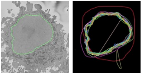
Figure 1: The Etch-a-Cell project. Left: an Electron Microscopy (EM) image of a cell. The real boundary of the tumor is marked in green. Right: multiple annotations by volunteers. Images taken from (Spiers et al. 2021).

$\begin{array}[]{c|c|cccc|c}i\leavevmode\nobreak\ \backslash\leavevmode\nobreak\ j&&1&2&3&4&d(\bm{s},\bm{z})\\ \hline\cr&t_{i}\leavevmode\nobreak\ \backslash\leavevmode\nobreak\ z_{j}&80&0&40&-10&\\ \hline\cr 1&55&81&6&41&-14&13.5\\ 2&80&89&-6&35&4&84.5\\ 3&100&105&-18&39&-5&243.7\\ 4&120&68&9&62&-10&177.2\\ 5&165&67&20&58&-20&248.2\\ \hline\cr UA(S)&&82&2.2&47&-9&14.7\\ \end{array}$

Table 1: An example of a dataset sampled from the AWG model. The bottom row is showing aggregated results using the unweighted mean. The rightmost column shows the error, i.e. the distance of every row from the ground truth.

g

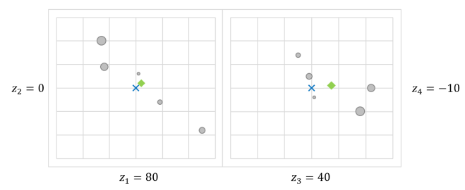
Figure 2: A graphical representation of Table 1 (for obvious reasons we use two 2-dimensional plots instead of a 4-dimensional one). The blue X marks the ground truth. Workers’ reports are marked by gray circles, whose size is proportional to $t_{i}$ (so smaller circles tend to be closer to the truth). The mean $\textsc{UA}(S)$ is marked by a green diamond.

We denote by $\mu_{\mathcal{T}}(\bm{z}):=E_{\bm{s}\sim\mathcal{Y}(\bm{z},{\mathcal{T}})}[d(\bm{s},\bm{z})]$ the mean fault, omitting ${\mathcal{T}}$ and/or $\bm{z}$ when clear from the context.

Distance measures can often be derived from an inner product. Formally, consider an arbitrary symmetric inner product space $(Z,\left\langle\cdot,\cdot\right\rangle)$. This induces a norm $\|\bm{x}\|^{2}:=\left\langle\bm{x},\bm{x}\right\rangle$ and a distance measure $d(\bm{x},\bm{y}):=\|\bm{x}-\bm{y}\|^{2}$ (not necessarily a metric). A special case of interest is the normalized Euclidean product on $Z=\mathbb{R}^{m}$, defined as $\left\langle\bm{x},\bm{y}\right\rangle_{E}:=\frac{1}{m}\sum_{j\leq m}x_{j}y_{j}$; and the corresponding normalized squared Euclidean distance (NSED), a natural way to capture the dissimilarity of two items (Carter, Morris, and Blashfield 1989). Note that the fault of a worker in the AWG model under NSED is her variance, as $f_{i}(\bm{z})=t_{i}$ for any $\bm{z}$.

Indeed:

$$f_{i} (\bm{z})=E_{\bm{s}_{i}\sim\mathcal{Y}(\bm{z},t_{i})}[d_{E}(\bm{s}_{i},\bm{z})]$$ (1)

$$=E_{\bm{s}_{i}\sim\mathcal{Y}(\bm{z},t_{i})}[\sum_{j\leq m}(s_{ij}-z_{j})^{2}]=VAR_{\bm{s}_{i}\sim\mathcal{Y}(\bm{z},t_{i})}[\bm{\epsilon}_{i}]=t_{i}.$$

Aggregation

Given an instance $\left\langle S,\bm{z}\right\rangle$, an aggregation function returns predicted labels $\hat{\bm{z}}$. We define the error as $d(\bm{z},\hat{\bm{z}})$. For example unweighted aggregation in the real-valued domain simply returns the mean of workers’ answers. The goal of truth discovery is to find algorithms that return labels with low expected error, see Table 1.

When the type of every worker is known, for many noise models there are accurate characterizations of the optimal aggregation functions. For example, the best linear unbiased estimator under the AWG model with NSED is taking the mean of workers’ answers, inversely weighted by their variance (Aitkin 1935).

3 Fault Estimation

Our key approach is relying on estimating $f_{i}$ using the average distance of worker $i$ from all other workers. Formally, we define $d_{ii^{\prime}}:=d(\bm{s}_{i},\bm{s}_{i^{\prime}})$, and the average pairwise distance is

$$\pi_{i}:=\frac{1}{n-1}\sum_{i^{\prime}\in N\setminus\{i\}}d_{ii^{\prime}}.$$ (2)

Next, we analyze the relation between $\pi_{i}=\pi_{i}(S)$ (which is a random variable) and $f_{i}$, which is an inherent property that is deterministically induced by the worker’s type. For an element $\bm{s}\in Z$ we consider the induced noise variable $\bm{\epsilon}_{\bm{s}}:=\bm{s}-\bm{z}$. We denote by $\tilde{\mathcal{Y}}(\bm{z},t)$ the distribution of $\bm{\epsilon}_{\bm{s}}$ (where $\bm{s}\sim\mathcal{Y}(\bm{z},t)$). Thus under NSED we have that $d(\bm{s},\bm{z})=\|\bm{\epsilon}_{\bm{s}}\|^{2}$.

We define $\bm{b}_{i}(\bm{z}):=E_{\bm{\epsilon}_{i}\sim\tilde{\mathcal{Y}}(\bm{z},t_{i})}[\bm{\epsilon}_{i}]$ as the bias of a type $i$ worker, and $\bm{b}_{{\mathcal{T}}}(\bm{z}):=E_{\bm{\epsilon}\sim\tilde{\mathcal{Y}}(\bm{z},{\mathcal{T}})}[\bm{\epsilon}]$ as the mean bias of the proto-population. E.g. in Euclidean space $\bm{b}_{i}(\bm{z})$ is a vector where $b_{ij}(\bm{z})>0$ if $i$ tends to overestimate the answer of question $j$, and negative values mean underestimation.

Our main conceptual result is an approximately linear connection between the expectations of $\pi_{i}$ and $d(\bm{s}_{i},\bm{z})$.

Theorem 1 (Anna Karenina Principle).

$$E_{S\sim\mathcal{Y}(\bm{z},{\mathcal{T}})^{n}}[\pi_{i}|t_{i},\bm{z}]=f_{i}(\bm{z})+\mu_{{\mathcal{T}}}(\bm{z})-2\left\langle\bm{b}_{i}(\bm{z}),\bm{b}_{{\mathcal{T}}}(\bm{z})\right\rangle.$$

We can also see this linear relation in three datasets (with different labels and distance measures) on Fig. 3.

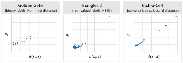
Figure 3: Realized average distance $\pi_{i}$ vs. error. Each point is a worker.

The proof is rather straight-forward, and is relegated to Appendix B, with examples in Appendix H. In particular it shows by direct computation that the expectation of $d_{ii^{\prime}}$ for every pair of workers is

$$E[d_{ii^{\prime}}|t_{i},t_{i^{\prime}},\bm{z}]=f_{i}(\bm{z})+f_{i^{\prime}}(\bm{z})-2\left\langle\bm{b}_{i}(\bm{z}),\bm{b}_{i^{\prime}}(\bm{z})\right\rangle.$$ (3)

Despite (or perhaps because of) its simplicity, the principle above is highly useful for estimating workers’ competence. If $\pi_{i}$ is roughly linearly increasing in $f_{i}$, a naïve approach to estimate $f_{i}$ from the data is by setting $\hat{f}_{i}$ to be some increasing function of $\pi_{i}$.

However there are several obstacles we need to overcome in order to get theoretical guarantees.

Concentration bounds

I.e., showing that w.h.p the average similarity is close to its expected value, and thus approximates the competence.

Dependency on the ground truth

As long as $E[\pi_{i}]$ depends on $\bm{z}$, we have a chicken and egg problem, since we do not know the truth. We will show conditions under which $E[\pi_{i}]$ does not depend on $\bm{z}$ at all.

Biases

The value depends on the bias $\bm{b}_{i}$ which is part of the unknown type. Estimating or bounding this bias is a major part of our work.

Population parameters

Another dependency is on $\mu_{{\mathcal{T}}}$ and $\bm{b}_{{\mathcal{T}}}$, which depend on the population. These parameters can often be easily guessed or estimated. We will also consider a conservative approach that assigns a default value of $0$.

For concreteness, we assume in the remainder of the paper, except where explicitly stated otherwise, that the inner product space $(Z,\left\langle\right\rangle)$ is $\mathbb{R}^{m}$, and $d$ is NSED.

Concentration bounds

How far is the empirical average $\pi_{i}$ from its expectation? We show that when the noise on all questions is independent and bounded, the probability of a large estimation error decreases linearly with the sample size $\min\{n,m\}$. For details see Appendix F.

Domain-independent bounds

What can be said without symmetry or other assumptions on the model? We argue that we can at least tell particularly poor workers from good workers.

Corollary 2.

Consider a “bad” worker $i^{*}$ with $f_{i^{*}}>9\mu_{\mathcal{T}}$, and a “good” worker $i^{**}$ with $f_{i^{**}}<\mu_{\mathcal{T}}$. Then $E[\pi_{i^{*}}]>E[\pi_{i^{**}}]$. No better separation is possible (i.e. there is an instance where all the inequalities become equalities).

The proof relies on the following lemma, which is itself a corollary of the Anna Karenina principle (Thm. 1) and the Cauchy-Schwarz inequality:

Lemma 3.

For any worker $i$ and any $\gamma\geq 0$, if $f_{i}=\gamma\mu$, then $E[\pi_{i}|t_{i}]\in(1\pm\sqrt{\gamma})^{2}\mu$.

Proof of Corollary 2.

By Lemma. 3, $E[\pi_{i^{**}}]\leq 4\mu<E[\pi_{i^{*}}]$.

Without further assumptions, this condition is tight. To see why, consider a population on $\mathbb{R}$ where $z=0$. The good worker $i^{**}$ provides the fixed report $s_{i^{**}}=-1$, the poor worker $i^{*}$ provides the fixed report $s_{i^{*}}=3-\delta$. However the measure of types $t_{i^{*}},t_{i^{**}}$ in ${\mathcal{T}}$ is 0, and w.p. 1 type $t^{\prime}$ is selected with a fixed report $s=1$. Note that $\mu=(s-z)=1$, and thus $f_{i^{**}}=1=\mu$ whereas $f_{i^{*}}=9=9\mu$.

However, the reports of $i^{*},i^{**}$ are completely symmetric around $1$, in the absence of more workers there is no way to distinguish between these two workers, by their disparity or otherwise. ∎

In the special case of interest when there are only two types of workers (a situation known as “Hammer-spammer” (Karger, Oh, and Shah 2011)), Lemma 3 enables us to separate good from bad workers even more easily. This essentially depends on the fraction of bad workers and on their bias. See Appendix B for details and proofs.

Symmetric Noise

A trivial implication of Theorem Theorem is when the average worker is unbiased:

Corollary 4 (Anna Karenina principle for zero bias).

If $\bm{b}_{\mathcal{T}}\!=\!0$ then $E[\pi_{i}|t_{i}]=f_{i}\!+\!\mu_{\mathcal{T}}$ for all $i$.

This means that given enough samples, we can retrieve workers’ exact fault level with high accuracy, by setting $\hat{f}_{i}:=\pi_{i}(S)-\hat{\mu}$. This will be important later on when we discuss aggregation.

What if we use other distance measures than NSED? Suppose that $d$ is an arbitrary distance metric over space $Z$, $\bm{z}\in Z$ is the ground truth, and $\bm{s}_{i}\in Z$ is the report of worker $i$. $f_{i}$ and $\pi_{i}$ are defined as before. Intuitively, we say that the noise model $\mathcal{Y}$ is symmetric if for every point $\bm{x}$ there is an equally-likely point that is on “the other side” of $\bm{z}$ (note that this in particular implies zero bias).

Theorem 5 (Anna Karenina principle for symmetric noise and distance metrics).

If $d$ is any distance metric and $\mathcal{Y}$ is symmetric, then $\max\{\mu,f_{i}\}\leq E[\pi_{i}|t_{i}]\leq\mu+f_{i}$.

An immediate corollary of Theorem 5 is that for poor workers with $f_{i}\geq\mu$, the average distance $\pi_{i}$ is a 2-approximation for $f_{i}$ (up to noise). See details and proof in Appendix D.

Domain-specific results

Binary labels

Kurvers et al. (2019) considered the average similarity of workers when answering a set of yes/no questions, and the type of a worker is her probability $p_{i}$ to answer correctly independently over each question, a model known as the one-coin model or the Dawid-Skene model.

They showed that the (expected) average similarity is an increasing linear function of $p_{i}$.

Interestingly, the result from (Kurvers et al. 2019) can also be obtained directly from Theorem 1, by plugging in the Hamming distance (which is just NSED on the binary cube $\{-1,1\}^{d}$ instead of $\mathbb{R}^{d}$). This result can also be easily extended to multiple-choice labels. For details see Appendix C.

Cosine similarity

When label vectors are normalized, we have that $d(\bm{x},\bm{y})=2(1-cos(\bm{x},\bm{y}))$, meaning that ranking workers by decreasing average cosine similarity (as suggested in (Kobayashi 2018)) is the same as ranking them by increasing average NSED. Our results above provide sufficient conditions for when this separates good workers from poor ones.

4 AWG Model and Maximum Likelihood

By imposing the same variance on all dimensions, the model assumes that questions are equally difficult.

Since AWG has no bias, we know from Cor. 4 that $E[\pi_{i}(S)|t_{i}]=f_{i}+\mu$. Thus if we have a good estimate $\hat{\mu}$ of $\mu$, setting $\hat{f}_{i}:=\pi_{i}-\hat{\mu}$ is a reasonable heuristic. In this section we show that under a slight relaxation of the AWG model, tweaking the heuristic above provides the MLE for $f_{i}$.

Denote $\bar{\mu}:=\frac{1}{2n}\sum_{i\in N}\pi_{i}(S)$, that is, half the average pairwise distance. Note that for unbiased workers, we have by Cor. 4 that $E[\frac{1}{n}\sum_{i\in N}\pi_{i}(S)]=2\mu$, and thus $\bar{\mu}$ is an unbiased estimator of $\mu$. We thus set $\hat{f}^{NP}_{i}:=\pi_{i}-\bar{\mu}$, where $NP$ stands for Naïve Proxy.

Computing the MLE

From Eq. (3) and zero-bias, we have that $E[d_{ii^{\prime}}|t_{i},t_{i^{\prime}}]=f_{i}+f_{i^{\prime}}$. However even under the AWG model, the pairwise distances are correlated. For the analysis, we will neglect these correlations, and assume that the pairwise distances are all independent conditional on workers’ types. More formally, under this ‘pairwise’ Additive White Gaussian (pAWG) model, $d_{ii^{\prime}}=f_{i}+f_{i^{\prime}}+\epsilon_{ii^{\prime}}$, where all of $\epsilon_{ii^{\prime}}$ are sampled i.i.d. from a normal distribution with mean 0 and unknown variance. Ideally, we would like to find ${\ddot{f}}:=(\hat{f}_{i})_{i\in N}$ that minimize the estimation errors $(\epsilon_{ii^{\prime}})$, which is an Ordinary Least Squares (regression) problem.

We next show how to derive a closed form solution for the maximum likelihood estimator of the fault $\vec{f}$, also allowing for a regularization term with coefficient $\lambda$. The theorem might have independent interest as it allows us to estimate a matrix created from adding a vector to itself (an “outer sum” matrix) from its off-diagonal entries.

Theorem 6.

Let $\lambda\geq 0$, and $D=(d_{ii^{\prime}})_{i,i^{\prime}\in N}$ be an arbitrary symmetric nonnegative matrix. Then

$$\operatorname{\text{argmin}}_{{\ddot{f}}}\!\!\!\!\!\!\!\!\sum_{i,i^{\prime}\in N:i\neq i^{\prime}}\!\!\!\!\!\!(\hat{f}_{i}+\hat{f}_{i^{\prime}}-d_{ii^{\prime}})^{2}+\lambda\|{\ddot{f}}\|^{2}_{2}=\frac{2(n-1)\vec{\pi}\!-\!\frac{8n(n-1)}{4n+\lambda-4}\bar{\mu}}{2n+\lambda-4}.$$

Our main technical result in this paper follows as a direct corollary of the above theorem, when the matrix $D$ represents pairwise distances:

Theorem 7.

For $\lambda=4$, the regularized maximum likelihood estimator of $\vec{f}$ in the pAWG model is proportional to ${\ddot{f}}^{NP}$.

That is, our heuristic estimate ${\ddot{f}}^{NP}$ is in fact the optimal solution of a regularized pAWG model.

By setting $\lambda=0$ (no regularization) we get a slight variation of this heuristic ${\ddot{f}}^{ML}:=\vec{\pi}-\frac{n}{n-1}\bar{\mu}$ (for ‘maximum likelihood’).

In Fig. 4 we compare implementations of our truth discovery algorithm (defined in Section 5, derived with different values of $\lambda$. As expected, more regularization leads to better performance on a small dataset, whereas the unregularized version is optimal in the limit.

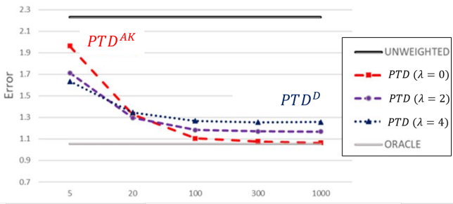
Figure 4: A comparison of the P-TD algorithm variants on a synthetic real-valued dataset. The x-axis shows the number of questions $m$, whereas the number of workers is fixed ($n=5$). ‘ORACLE’ weighs workers according to their true competence.

Proof of Theorem 6 for $\lambda=0$.

Let $P$ be a list of all $n^{2}-n$ ordered pairs of $[n]$ (without the main diagonal) in arbitrary order. Setting $\lambda=0$, we are left with the following least squares equation:

$$\min_{{\ddot{f}}}\sum_{i,i^{\prime}}(\hat{f}_{i}+\hat{f}_{i^{\prime}}-d_{ii^{\prime}})^{2}=\min_{{\ddot{f}}}\|A{\ddot{f}}-\bm{d}\|_{2}^{2},\vspace{-0mm}$$

where $A$ is a $|P|\times n$ matrix with $a_{ki}=1$ iff $i\in P_{k}$, and $\bm{d}$ is a $|P|$-length vector with $d_{k}=d_{i{i^{\prime}}}$ for $P_{k}=(i,{i^{\prime}})$.

Fortunately, $A$ has a very specific structure that allows us to obtain the above closed-form solution. Note that every row of $A$ has exactly two ‘1’ entries, in the row index $i$ and column index ${i^{\prime}}$ of $P_{k}$; the total number of ‘1’ is $2(n^{2}-n)$; there are $2n-2$ ones in every column; and every two distinct columns $i,{i^{\prime}}$ share exactly two non-zero entries (at rows $k$ s.t. $P_{k}=(i,{i^{\prime}})$ and $P_{k}=({i^{\prime}},i)$). This means that $(A^{T}A)$ has $2n-2$ on the diagonal and $2$ in any other entry.

The optimal solution for ordinary least squares is obtained at ${\ddot{f}}$ such that $(A^{T}A){\ddot{f}}=A^{T}\bm{d}$. By the structure of $A$:

$$[A^{T}\bm{d}]_{i}=2\sum_{{i^{\prime}}\neq i}d_{i{i^{\prime}}}=2\pi_{i},\vspace{-0mm}$$ (4)

and

$$[(A^{T}A){\ddot{f}}]_{i}=2(n-2)\hat{f}_{i}+2\sum_{i^{\prime}\in N}\hat{f}_{i^{\prime}}.$$ (5)

Denote

$$\alpha:=\sum_{i\in N}[A^{T}\bm{d}]_{i}=\sum_{i\in N}2\sum_{{i^{\prime}}\neq i}d_{i{i^{\prime}}}=4n(n-1)\bar{\mu},\vspace{-0mm}$$ (6)

then by Eq. (5):

$$\alpha =\sum_{i\in N}[(A^{T}A){\ddot{f}}]_{i}=\sum_{i\in N}[2(n-2)\hat{f}_{i}+2\sum_{i^{\prime}\in N}\hat{f}_{i^{\prime}}]$$ (7)

$$=2(n-2)\sum_{i\in N}f_{i}+2\sum_{i^{\prime}\in N}f_{i^{\prime}}(\sum_{i\in N}1)=4(n-1)\sum_{i\in N}\hat{f}_{i}.$$

We can now write the $n$ linear equations as

$$2(n-1)\pi_{i}\!=\![A^{T}\bm{d}]_{i}\!=\![(A^{T}A){\ddot{f}}]_{i}$$ (By Eqs. (4),(5))

$$=(2n-4)\hat{f}_{i}+2\sum_{i^{\prime}\in N}\hat{f}_{i^{\prime}} \iff$$

$$(n-1)\pi_{i}=(n-2)\hat{f}_{i}+\sum_{i^{\prime}\in N}\hat{f}_{i^{\prime}} \iff$$

$$\hat{f}_{i}=\frac{\pi_{i}}{n\!-\!2}-\frac{1}{n\!-\!2}\sum_{i^{\prime}\in N}\hat{f}_{i^{\prime}}=\frac{\pi_{i}}{n\!-\!2}-\frac{1}{n\!-\!2}\frac{\alpha}{4(n\!-\!1)}$$

$$\stackrel{{\scriptstyle Eq.\leavevmode\nobreak\ \eqref{eq:alpha1}}}{{=}}\frac{n-1}{n-2}\pi_{i}-\frac{n}{n-2}\bar{\mu}=\frac{n-1}{n-2}\hat{f}^{ML}_{i},$$

as required, since $\frac{n-1}{n-2}$ is a constant. ∎

5 Aggregation

Our Proximity-based Truth Discovery (P-TD) algorithm is a direct adaptation of the Anna Karenina principle. The idea is very simple:

1. Compute the average distance [or similarity] $\pi_{i}$ of every worker;

2. Estimate fault [or competence] ${\ddot{f}}$ from $\vec{\pi}$;

3. Aggregate answers, giving higher weight to workers with low fault [high competence].

Input: Dataset $S\in\mathbb{R}^{n\times m}$.

Output: Est. fault levels ${\ddot{f}}\in\mathbb{R}^{n}$; answers $\hat{\bm{z}}\in\mathbb{R}^{m}$.

Compute $d_{ii^{\prime}}\leftarrow d(\bm{s}_{i},\bm{s}_{i^{\prime}})$ for every pair of workers;

for each worker $i\in N$ do

      set $\pi_{i}\leftarrow\frac{1}{n-1}\sum_{i^{\prime}\neq i}d_{ii^{\prime}}$;

       // Step 1

     

      end for

     Set $\bar{\mu}\leftarrow\frac{1}{2n}\sum_{i\in N}\pi_{i}$;

      for each worker $i\in N$ do

           Set $\hat{f}_{i}\leftarrow\pi_{i}-\frac{n}{n-1}\bar{\mu}$;

            // Step 2

           Set $w_{i}\leftarrow\frac{1}{\hat{f}_{i}}$;

          

           end for

          Set $\hat{\bm{z}}\leftarrow\frac{\sum_{i}w_{i}\bm{s}_{i}}{\sum_{i}w_{i}}$;

            // Step 3

           return $({\ddot{f}},\hat{\bm{z}})$;

ALGORITHM 1 (P-TD^D) for real-valued data

Our default implementation (denoted P-TD^D) simply sets weights proportional to the estimated competence, which is in turn proportional to the average similarity, as in (Kobayashi 2018; Kurvers et al. 2019).

As we make more assumptions on the structure of labels and the statistical model, we can use an appropriate Anna-Karenina theorem to improve Step 2, resulting in a domain-specific implementation P-TD^AK. For example, Alg. 1 shows the implementation for the real-valued domain, where Step 2 is based on ${\ddot{f}}^{ML}$ defined in Sec. 4, and Step 3 is based on (Aitkin 1935). See Appendix G for details on other domain-specific implementations.

Lastly, we can iteratively repeat the process by computing the weighted average distance to other workers. This iterative P-TD algorithm is denoted by iP-TD.

6 Empirical Evaluation

Algorithms

We compare the predicted label accuracy of our algorithms (P-TD^D,P-TD^AK,iP-TD) to unweighted aggregation (UA); to three general-domain algorithms: MAS (Braylan and Lease 2020), TOP2 and EXP (Kawase, Kuroki, and Miyauchi 2019); and to domain-specific algorithms: CRH (Li et al. 2014b), IBP (Karger, Oh, and Shah 2011), DS (Dawid and Skene 1979), EVD (Parisi et al. 2014), CATD (Li et al. 2014a), GTM (Zhao and Han 2012), and KDE (Wan et al. 2016).

Datasets

We used the following datasets from five different domains. We write the used distance measure in each domain in brackets.

Categorical (Hamming distance):

GG, DOGS, FLAGS (Shah and Zhou 2015); Predict (Mandal, Radanovic, and Parkes 2020) (we used data from Oct.8, under all four treatments); and all six categorical datasets from (Kawase, Kuroki, and Miyauchi 2019). We used weighted majority for aggregation.

Real-valued (NSED):

BUILDINGS (collected for this paper); TRI (Hart et al. 2018); and EMO (Snow et al. 2008). Answers aggregated using weighted mean.

Ranking (Kendall-tau):

DOTS and PUZZ contain subjective rankings of four images of dots / 8-puzzle boards, according to the number of dots they contain / number of steps from solution  (Mao, Procaccia, and Chen 2013). We also extracted the ranking information from BUILDINGS. For aggregation, we used nine different ordinal voting rules, see Appendix for details.

Language (GLEU):

The TRANSL dataset contains English translations of Japanese sentences (Braylan and Lease 2020). The distance measure we used is GLEU, and there is no aggregation (best worker is selected).

Outlines (Jaccard):

The Etch-a-Cell dataset contains bitmaps of the outline of a tumor in 2D slices of a cell (Spiers et al. 2021) (see Fig. 1). We use Jaccard distance on the filled shapes, and aggregate labels using pixelwise-majority.

In addition we generated synthetic datasets using the AWG model (real-valued); the one-coin model (categorical); and Mallows model (ranking). In the HS datasets there are 20% ‘hammers’.

A detailed description of algorithms’ implementation and datasets is in Appendix H.

To obtain robust results we sampled $n$ workers and $m$ questions without repetition from each dataset (real or synthetic), and repeated the process at least 1000 times for every combination.

Categorical	k	CRH	IBP	DS	EVD	EXP	TOP2	MAS	P-TDD	P-TDAK	iP-TD
SYN.HS	2	-14%	+6%	-23%	-20%	-15%	-13%	-17%	-21%	-24%	-24%
SYN.N	2	-4%	+12%	-9%	-6%	-7%	-8%	-5%	-7%	-9%	-9%
GG	2	-8%	-15%	-19%	-10%	-14%	-20%	-14%	-14%	-18%	-18%
Pred.T1	2	-1%	+9%	-1%	-1%	-1%	+0%	-1%	-1%	-1%	-1%
Pred.T2	2	-0%	+10%	+0%	-1%	-1%	+1%	+0%	-0%	-1%	-1%
Pred.T3	2	-1%	+8%	-1%	-1%	-0%	+1%	-1%	-2%	-2%	-2%
Pred.T4	2	-1%	+7%	-2%	-4%	-1%	-1%	-2%	-3%	-3%	-3%
SYN	4	-18%	$-$	$-$	$-$	-22%	-29%	-28%	-33%	-33%	-41%
DOGS	10	-1%	$-$	$-$	$-$	-2%	+0%	-3%	-4%	-4%	-4%
FLAGS	4	-17%	$-$	$-$	$-$	-29%	-31%	-27%	-21%	-22%	-30%
Chinese	2	-2%	$-$	$-$	$-$	-1%	-3%	-4%	-4%	-4%	-5%
English	2	-1%	$-$	$-$	$-$	-1%	-1%	-1%	-1%	-1%	-1%
IT	4	-3%	$-$	$-$	$-$	-4%	-5%	-6%	-5%	-5%	-7%
Medicine	4	-3%	$-$	$-$	$-$	-13%	-16%	-9%	-8%	-8%	-12%
Pokemon	6	-11%	$-$	$-$	$-$	-25%	-27%	-17%	-22%	-22%	-27%
Science	5	-1%	$-$	$-$	$-$	+1%	+1%	-1%	-3%	-3%	-3%
Real-valued		CRH	CATD	GTM	KDE	EXP	TOP2	MAS	P-TDD	P-TDAK	iP-TD
SYN.N	$-$	-23%	-27%	-14%	+6%	-7%	-11%	+4%	-20%	-41%	-25%
BUILD	$-$	-9%	+5%	-9%	+1%	-8%	+12%	+4%	-7%	-7%	-11%
TRI1	$-$	-19%	-7%	-14%	-4%	-17%	-3%	-8%	-17%	-10%	-20%
TRI2	$-$	-9%	-6%	-5%	-4%	-11%	-12%	+1%	-7%	-4%	-11%
EMO	$-$	+1%	+18%	+1%	+26%	+5%	+22%	+3%	+0%	+5%	+2%

Table 2: Results (RI) on categorical and real-valued datasets, with $n=10$ workers and $m=15$ questions (more sizes in the appendix). The best result in each row is underlined, and results that are not statistically different (within 95% confidence interval in a paired t-test) are marked in bold. Results in gray are worse than unweighted aggregation.

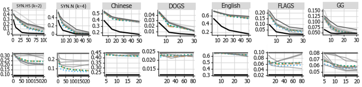
Figure 5: The error on some of the real world datasets as we increase the number of voters $n$ with fixed $m=15$ as in the table (top row), or vary the number of questions $m$ with fixed $n=10$ (bottom row). The black line is the error of an Oracle who knows the true fault values $f$ and uses optimal weights. The thin gray lines are all competing algorithms.

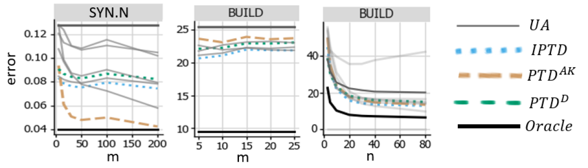
Figure 6: The error on real-valued datasets as we vary $m$ (keeping $n=10$) or $n$ (keeping $m=15$).

Ranking	v. rule	EXP	TOP2	MAS	P-TDD	iP-TD
SYN.HS	Borda	-5%	-24%	-14%	-4%	-10%
SYN.N	Borda	-3%	+6%	+1%	-4%	-6%
BUILD	Borda	+0%	+0%	+0%	-0%	+0%
DOTS3	Borda	+2%	+7%	+2%	-1%	+1%
DOTS5	Borda	+1%	+9%	+4%	-1%	-1%
DOTS7	Borda	+1%	+13%	+5%	-3%	-2%
DOTS9	Borda	-3%	+7%	-1%	-6%	-10%
PUZZ5	Borda	+1%	+1%	+8%	-2%	-2%
PUZZ7	Borda	-10%	-7%	-18%	-15%	-20%
PUZZ9	Borda	+6%	+48%	+14%	-5%	-1%
PUZZ11	Borda	-0%	+6%	+3%	-3%	-3%
SYN.N	Plurality	-4%	-2%	-5%	-4%	-5%
BUILD	Plurality	-1%	+20%	-2%	-6%	-6%
DOTS3	Plurality	+2%	+14%	+2%	-2%	-1%
PUZZ5	Plurality	+1%	+12%	+1%	-3%	-2%
SYN.N	Copeland	-12%	-37%	-25%	-27%	-29%
BUILD	Copeland	-12%	-7%	-17%	-27%	-27%
DOTS3	Copeland	+0%	+0%	-1%	-0%	-0%
PUZZ5	Copeland	-7%	-12%	-16%	-19%	-18%
Complex
TRANSL	best v.	-2%	-3%	-3%	-4%	-4%
ETCH	best v.	-28%	-39%	-39%	-43%	-42%
ETCH	bit. maj.	-1%	-2%	-4%	-2%	-2%

Table 3: Results (RI) for rankings datasets, under three different voting rules ($n=10$, four ranked alternatives), and on the other complex annotation datasets.

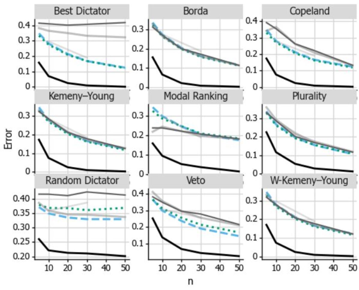
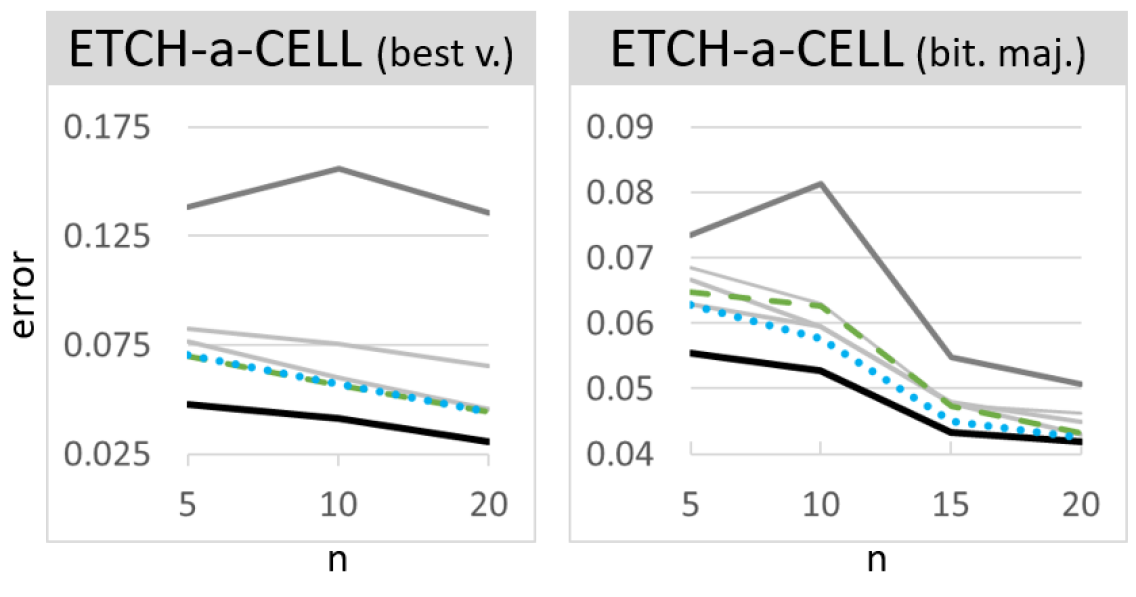
Figure 7: Top: error on DOTS3 under nine different voting rules. Bottom: error on Etch-a-Cell as number of workers grows.

Evaluation

The error of every algorithm is the distance (as specified above) to the ground truth, averaged over all samples of certain size of a particular dataset.

In the tables, we compute for each algorithm its Relative Improvement $RI(Alg):=\frac{Err(Alg)-Err(\textsc{UA})}{Err(Alg)+Err(\textsc{UA})}$, where UA serves as a baseline. Thus RI is in the range $[-1,1]$ where negative numbers mean improvement over UA.

In some cases we see that one algorithm has slightly higher average error (on the graphs) but lower RI, or that the gap in RI is more substantial. This is since the graphs average over instances of varying difficulty, so instances with high baseline error have more effect.

Results

Fig. 5 and Table 2 (and more in Appendix H) show results on categorical and real-valued data, where there are many specialized algorithms. We can see that there is no single ‘state-of-the-art’, as algorithms that do well on some datasets may have poor performance on other data, or for a different number of voters/questions.

Yet for moderate $n$ and $m$, all three versions of our P-TD consistently provide good results over almost all datasets, usually beating the three general-domain algorithms, and doing roughly at par with the best specialized ones. We can also see that on synthetic real-valued data with Gaussian noise, the provably-optimal P-TD^D is also best in practice.

On real datasets, our iP-TD is usually better, and as $n$ and $m$ increase sometimes one of the specialized algorithms takes over. Intuitively, real datasets may often have a some correlation in poor workers’ errors. Iterative algorithms, such as our iP-TD and some of the existing algorithms, are able to overcome this since they gradually rely more on the largest and most consistent set of workers.

The real strength of our approach shows when labels are more complex. Table 3 and Fig. 7 show how our simple algorithms are consistently better than the other three algorithms both on ranking data and on both complex annotation tasks. Results also show that P-TD yields substantial improvement regardless of the voting rule in use. Moreover, while the other algorithms work better on some datasets, they are highly unstable and often perform worse than the baseline.

7 Conclusion

Average proximity can be used as a general scheme to estimate workers’ competence in a broad range of truth discovery and crowdsourcing scenarios. Due to the “Anna Karenina principle,” we expect the answers of competent workers to be much closer to others, than those of incompetent workers, even under very weak assumptions on the domain and the noise model. Under more explicit assumptions, the average distance accurately estimates the true competence.

The above results suggest an extremely simple, general and practical algorithm for truth-discovery (the P-TD algorithm), that weighs workers by their average proximity to others, and can be combined with most aggregation methods. This is particularly useful in the context of existing crowdsourcing systems where the aggregation rule may be subject to constraints due to legacy, simplicity, explainability, legal, or other considerations (e.g. a voting rule with certain axiomatic properties). In addition, average proximity is simple and flexible enough so we can modify it to deal with challenges outside the scope of the current paper, such as partial data (Dalvi et al. 2013; Karger, Oh, and Shah 2011; Li et al. 2014a); semi-supervised learning (Yin and Tan 2011); or worker’s competence that varies across task types (Braylan and Lease 2020).

Despite its simplicity, the P-TD algorithm substantially improves the outcome compared to unweighted aggregation. It is also competitive with other, more sophisticated algorithms, especially in the common case of moderate input size. We thus conclude that the average similarity heuristic is indeed a frustratingly easy—and practical—tool for crowdsourcing.

An obvious shortcoming of P-TD is that a group of workers that submit similar labels (e.g. by acting strategically) can boost their own weights. Future work will consider how to identify and/or mitigate the affect of such groups.

We denote by $\left\llbracket C\right\rrbracket$ the indicator variable of a true/false condition $C$.

Throughout the appendix, the disparity of a worker refers to the her average distance to other workers, i.e. $\pi_{i}$.

We denote by $\mu_{\mathcal{T}}(\bm{z}):=E_{\bm{s}\sim\mathcal{Y}(\bm{z},{\mathcal{T}})}[d(\bm{s},\bm{z})]$ the mean fault, omitting ${\mathcal{T}}$ and/or $\bm{z}$ when clear from the context.

Appendix A A Detailed Graphical Example

Recall our running example from the main text, where we sampled the fault (i.e. the variance) of five workers from $U[50,200]$.

For each worker we independently sampled her answers as $\bm{s}_{i}=\bm{z}+\bm{\epsilon}_{i}$, where according to the AWG model, each $\epsilon_{i,j}$ is sampled from a Normal distribution with mean $0$ and variance $t_{i}$.

The reports of the answers on the for real-valued questions are shown in Table 4 and also graphically in Figure 8.

For example, to calculate the error of worker 1, we average the squared distance over all four questions/dimensions:

$$d_{E}(\bm{x}_{1},\bm{z})=\frac{1}{4}((81-80)^{2}+(6-0)^{2}+(41-40)^{2}+(-14-(-10))^{2})=\frac{1}{4}(1+36+1+16)=13.5.$$

We can see that workers with lower variance (smaller circles) tend to be closer to the truth but are not necessarily closer. The last line shows the Oracle Aggregation, which is the weighted mean with weights inversely proportional to $t_{i}$. We see that it is indeed closer to the ground truth in this example.

$\begin{array}[]{c|c|cccc|c}i\leavevmode\nobreak\ \backslash\leavevmode\nobreak\ j&&1&2&3&4&d(\bm{s},\bm{z})\\ \hline\cr&t_{i}\leavevmode\nobreak\ \backslash\leavevmode\nobreak\ z_{j}&80&0&40&-10&\\ \hline\cr 1&55&81&6&41&-14&13.5\\ 2&80&89&-6&35&4&84.5\\ 3&100&105&-18&39&-5&243.7\\ 4&120&68&9&62&-10&177.2\\ 5&165&67&20&58&-20&248.2\\ \hline\cr UA(S)&&82&2.2&47&-9&14.7\\ OA(S)&&83.6&0.9&44.3&-8.3&8.9\\ \end{array}$

Table 4: An example of a dataset sampled from the AWG model. The bottom row is showing aggregated results using the unweighted mean. The rightmost column shows the error, i.e. the distance of every row from the ground truth using NSED. This is the same table as Table 1 in the main text. We also added a row for the Oracle Aggregation.

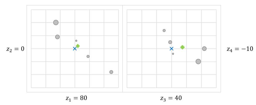
Figure 8: A graphical representation of Table 4 (for obvious reasons we use two 2-dimensional plots instead of a 4-dimensional one). The blue X marks the ground truth. Workers’ reports are marked by gray circles, whose size is proportional to $t_{i}$ (so smaller circles tend to be closer to the truth). The mean $\textsc{UA}(S)$ is marked by a green diamond.

Appendix B General Anna Karenina Theorem

Consider an inner product space with a symmetric inner product $\left\langle,\right\rangle$. As usual, the norm $\|\bm{x}\|$ is a shorthand for $\sqrt{\left\langle\bm{x},\bm{x}\right\rangle}$.

Theorem 1.

$$E_{S\sim\mathcal{Y}(\bm{z},{\mathcal{T}})^{n}}[\pi_{i}(S)|t_{i},\bm{z}]=f_{i}(\bm{z})+\mu_{{\mathcal{T}}}(\bm{z})-2\left\langle\bm{b}_{i}(\bm{z}),\bm{b}_{{\mathcal{T}}}(\bm{z})\right\rangle.$$

Proof.

$$E_{S\sim\mathcal{Y}(\bm{z},{\mathcal{T}})^{n}} [\pi_{i}(S)|t_{i},\bm{z}]=E_{S\sim\mathcal{Y}(\bm{z},{\mathcal{T}})^{n}}[\frac{1}{n-1}\sum_{i^{\prime}\neq i}\|\bm{s}_{i}-\bm{s}_{i^{\prime}}\|^{2}|t_{i},\bm{z}]$$

$$=E_{S\sim\mathcal{Y}(\bm{z},{\mathcal{T}})^{n}}[\frac{1}{n-1}\sum_{i^{\prime}\neq i}\|\bm{s}_{i}-\bm{z}-(\bm{s}_{i^{\prime}}-\bm{z})\|^{2}|t_{i},\bm{z}]$$

$$=E_{S\sim\mathcal{Y}(\bm{z},{\mathcal{T}})^{n}}[\frac{1}{n-1}\sum_{i^{\prime}\neq i}\|\bm{s}_{i}-\bm{z}\|^{2}+\|\bm{s}_{i^{\prime}}-\bm{z}\|^{2}-2\langle\,\bm{s}_{i}-\bm{z},\bm{s}_{i^{\prime}}-\bm{z}\rangle|t_{i},\bm{z}]$$

$$=E_{\bm{s}_{i}\sim\mathcal{Y}(\bm{z},t_{i})}[\frac{1}{n-1}\sum_{i^{\prime}\neq i}\|\bm{s}_{i}-\bm{z}\|^{2}|t_{i},\bm{z}]+E_{S\sim\mathcal{Y}(\bm{z},{\mathcal{T}})^{n-1}}[\frac{1}{n-1}\sum_{i^{\prime}\neq i}\|\bm{s}_{i^{\prime}}-\bm{z}\|^{2}|t_{i},\bm{z}]$$

$$\qquad\qquad-2E_{S\sim\mathcal{Y}(\bm{z},{\mathcal{T}})^{n}}[\frac{1}{n-1}\sum_{i^{\prime}\neq i}\langle\,\bm{s}_{i}-\bm{z},\bm{s}_{i^{\prime}}-\bm{z}\rangle|t_{i},\bm{z}]$$

$$=f_{i}(\bm{z})+\frac{1}{n-1}E_{t_{i^{\prime}}\sim\tau}[\sum_{i^{\prime}\neq i}E_{s_{i^{\prime}}\sim\mathcal{Y}(\bm{z},t_{i^{\prime}})}[\|\bm{s}_{i^{\prime}}-\bm{z}\|^{2}|t_{i^{\prime}},\bm{z}]|\bm{z}]$$

$$\qquad\qquad-2\frac{1}{n-1}E_{t_{i}\sim\tau}[\sum_{i^{\prime}\neq i}E_{{\bm{s}_{i}\sim\mathcal{Y}(\bm{z},t_{i})},{s_{i^{\prime}}\sim\mathcal{Y}(\bm{z},t_{i^{\prime}})}}[\langle\,\bm{s}_{i}-\bm{z},\bm{s}_{i^{\prime}}-\bm{z}\rangle|t_{i^{\prime}},t_{i},\bm{z}]|t_{i},\bm{z}]$$

$$=f_{i}(\bm{z})+\frac{1}{n-1}\sum_{i^{\prime}\neq i}E_{S\sim\mathcal{Y}(\bm{z},{\mathcal{T}})}[f_{i^{\prime}}|\bm{z}]$$

$$\qquad\qquad-2\frac{1}{n-1}\sum_{i^{\prime}\neq i}E_{t_{i}\sim\tau}[\langle\,E_{\bm{s}_{i}\sim\mathcal{Y}(\bm{z},t_{i})}[\bm{s}_{i}-\bm{z}|t_{i},\bm{z}],E_{\bm{s}_{i^{\prime}}\sim\mathcal{Y}(\bm{z},t_{i^{\prime}})}[\bm{s}_{i^{\prime}}-\bm{z}|t_{i^{\prime}},\bm{z}]\rangle|t_{i},\bm{z}]$$

$$=f_{i}(\bm{z})+\mu_{\mathcal{T}}(\bm{z})$$

$$\qquad\qquad-2\frac{1}{n-1}\sum_{i^{\prime}\neq i}\langle\,E_{t_{i}\sim\tau}[E_{\bm{s}_{i}\sim\mathcal{Y}(\bm{z},t_{i})}[\bm{s}_{i}-\bm{z}|t_{i},\bm{z}]|t_{i},\bm{z}],E_{t_{i}\sim\tau}[E_{\bm{s}_{i^{\prime}}\sim\mathcal{Y}(\bm{z},t_{i^{\prime}})}[\bm{s}_{i^{\prime}}-\bm{z}|t_{i^{\prime}},\bm{z}]|t_{i},\bm{z}]\rangle$$

$$=f_{i}(\bm{z})+\mu_{\mathcal{T}}(\bm{z})$$

$$\qquad\qquad-2\frac{1}{n-1}\sum_{i^{\prime}\neq i}\langle\,E_{\bm{s}_{i}\sim\mathcal{Y}(\bm{z},t_{i})}[\bm{s}_{i}-\bm{z}|t_{i},\bm{z}],E_{S\sim\mathcal{Y}(\bm{z},{\mathcal{T}})}[\bm{b}_{i^{\prime}}(\bm{z})|\bm{z}]\rangle$$

$$=f_{i}(\bm{z})+\mu_{\mathcal{T}}(\bm{z})-2\left\langle\bm{b}_{i}(\bm{z}),\bm{b}_{{\mathcal{T}}}(\bm{z})\right\rangle$$

∎

Model-free bounds

In the following lemmas, all parameters ($\bm{b}_{i},f_{i},\mu$) may depend on $\bm{z}$ as in Theorem 1. We omit the $\bm{z}$ argument for easier reading.

Lemma 8.

For all $i$, $|\left\langle\bm{b}_{i},\bm{b}_{{\mathcal{T}}}\right\rangle|\leq\sqrt{f_{i}}\sqrt{\mu}$.

Proof.

Due to Cauchy-Schwarz inequality,

$$|\left\langle\bm{b}_{i},\bm{b}_{{\mathcal{T}}}\right\rangle| \leq\|\bm{b}_{i}\|\cdot\|\bm{b}_{{\mathcal{T}}}\|=\sqrt{\frac{1}{m}\sum_{j=1}^{m}b_{ij}}\cdot\sqrt{\frac{1}{m}\sum_{j=1}^{m}b_{{\mathcal{T}},j}}=\sqrt{\frac{1}{m}\sum_{j=1}^{m}(b_{ij})^{2}}\cdot\sqrt{\frac{1}{m}\sum_{j=1}^{m}(b_{{\mathcal{T}},j})^{2}}$$

$$=\sqrt{\frac{1}{m}\sum_{j=1}^{m}(E_{\bm{s}_{i}\sim\mathcal{Y}_{i}}[s_{ij}-z_{j}])^{2}}\cdot\sqrt{\frac{1}{m}\sum_{j=1}^{m}(E_{t\sim{\mathcal{T}}}E_{\bm{s}\sim\mathcal{Y}(t)}[s_{j}-z_{j}])^{2}}$$

By Jensen inequality and convexity of the square function,

$$\leq\sqrt{\frac{1}{m}\sum_{j=1}^{m}E_{\bm{s}_{i}\sim\mathcal{Y}_{i}}[(s_{ij}-z_{j})^{2}]}\cdot\sqrt{\frac{1}{m}\sum_{j=1}^{m}E_{t\sim{\mathcal{T}}}E_{\bm{s}\sim\mathcal{Y}(t)}[(s_{j}-z_{j})^{2}]}$$

$$\leq\sqrt{E_{\bm{s}_{i}\sim\mathcal{Y}_{i}}[\frac{1}{m}\sum_{j=1}^{m}(s_{ij}-z_{j})^{2}]}\cdot\sqrt{E_{t\sim{\mathcal{T}}}E_{\bm{s}\sim\mathcal{Y}(t)}[\frac{1}{m}\sum_{j=1}^{m}(s_{j}-z_{j})^{2}]}$$

$$\leq\sqrt{E_{\bm{s}_{i}\sim\mathcal{Y}_{i}}[d(\bm{s}_{i},\bm{z})]}\cdot\sqrt{E_{t\sim{\mathcal{T}}}E_{\bm{s}\sim\mathcal{Y}(t)}[d(\bm{s},\bm{z})]}\leq\sqrt{f_{i}}\cdot\sqrt{\mu},$$

as required. ∎

The following lemma is another corollary of the Anna Karenina principle.

Lemma 3. For any worker $i$ and any $\alpha\geq 0$, if $f_{i}=\alpha\mu$, then $E[\pi_{i}]\in(1\pm\sqrt{\alpha})^{2}\mu$.

Proof.

For the upper bound,

$$E[\pi_{i}] =f_{i}+\mu-2\left\langle\bm{b}_{i},\bm{b}_{{\mathcal{T}}}\right\rangle$$ (By Thm. 1)

$$\leq f_{i}+\mu+2\sqrt{f_{i}}\sqrt{\mu}$$ (By Lemma 8)

$$\leq\alpha\mu+\mu+2\sqrt{\alpha\mu}\sqrt{\mu}=(1+\alpha+2\sqrt{\alpha})\mu=(1+\sqrt{\alpha})^{2}\mu. f_{i}\leq\alpha\mu$$ (since )

The proof of the lower bound is symmetric. ∎

Corollary 2. Consider a “poor” worker $i^{*}$ with $f_{i^{*}}>9\mu_{\mathcal{T}}$, and a “good” worker $i^{**}$ with $f_{i^{**}}<\mu_{\mathcal{T}}$. Then $E[\pi_{i^{**}}]<E[\pi_{i^{*}}]$. No better separation is possible.

Proof.

By Lemma. 3, $E[\pi_{i^{**}}]\leq 4\mu<E[\pi_{i^{*}}]$.

Without further assumptions, this condition is tight. To see why, consider a population on $\mathbb{R}$ where $z=0$. The good worker $i^{**}$ provides the fixed report $s_{i^{**}}=-1$, the poor worker $i^{*}$ provides the fixed report $s_{i^{*}}=3-\delta$. However the measure of types $t_{i^{*}},t_{i^{**}}$ in ${\mathcal{T}}$ is 0, and w.p. 1 type $t^{\prime}$ is selected with a fixed report $s=1$. Note that $\mu=(s-z)=1$, and thus $f_{i^{**}}=1=\mu$ whereas $f_{i^{*}}=9=9\mu$.

However, the reports of $i^{*},i^{**}$ are completely symmetric around $1$, in the absence of more workers there is no way to distinguish between these two workers, by their disparity or otherwise. ∎

Corollary 9.

Suppose there are two types of workers, with $f^{P}>f^{H}$. For any spammer $i^{P}$ and hammer $i^{H}$, if any of the following conditions apply, then $E[\pi_{i^{P}}]>E[\pi_{i^{H}}]$:

1. $(b^{H})=0$ and $\alpha<\frac{f^{P}-f^{H}}{2(b^{P})^{2}}$;

2. $f^{H}=0$ and $\alpha<0.5$;

3. $f^{P}-f^{H}>(b^{P})^{2}-(b^{H})^{2}$;

4. $b^{P}\leq b^{H}$.

Intuitively, this means that it is easy to distinguish hammers from spammers as there are fewer spammers; as the difference in competence becomes larger; and as the spammers are less biased.

Proof.

Denote by $\beta:=\left\langle\bm{s}^{P},\bm{s}^{H}\right\rangle$ the amount of agreement in the bias of hammers and spammers.

For every spammer $i^{P}$

$$E[\pi_{i}|t_{i}=P] =f_{i}+\mu-2\left\langle\bm{b}_{i},\bm{b}_{{\mathcal{T}}}\right\rangle$$

$$=f^{P}+\alpha f^{P}-2\left\langle\bm{s}^{P},\alpha\bm{s}^{P}+(1-\alpha)\bm{s}^{H}\right\rangle$$

$$=f^{P}+\alpha f^{P}-\alpha 2\left\langle\bm{s}^{P},\bm{s}^{P}\right\rangle-(1-\alpha)2\left\langle\bm{s}^{P},\bm{s}^{H}\right\rangle$$

$$=f^{P}+\alpha f^{P}-2\alpha(b^{P})^{2}-(1-\alpha)2\left\langle\bm{s}^{P},\bm{s}^{H}\right\rangle$$

$$=f^{P}+\alpha f^{P}-2\alpha(b^{P})^{2}-2(1-\alpha)\beta.$$ (8)

Similarly, it applies for every hammer $i^{H}$:

$$E[\pi_{i}|t_{i}=H] =f_{i}+\mu-2\left\langle\bm{b}_{i},\bm{b}_{{\mathcal{T}}}\right\rangle$$

$$=f^{H}+\alpha f^{P}-2\left\langle\bm{s}^{H},\alpha\bm{s}^{P}+(1-\alpha)\bm{s}^{H}\right\rangle$$

$$=f^{H}+\alpha f^{P}-2\alpha\beta-2(1-\alpha)(b^{H})^{2}.$$ (9)

(a) Follows immediately from Eqs. (8),(9), since $\beta=0$.

(b) Suppose $f^{H}=0$, then Condition (a) is implied, since $\frac{f^{P}-f^{H}}{2p^{2}}=\frac{f^{P}}{2p^{2}}\geq\frac{(b^{P})^{2}}{2(b^{P})^{2}}=\frac{1}{2}$.

(c) We note that due to Cauchy-Schwartz inequality,

$$|\beta|=|\left\langle\bm{s}^{P},\bm{s}^{H}\right\rangle|\leq\|\bm{s}^{P}\|\cdot\|\bm{s}^{H}\|=(b^{P})\cdot(b^{H})=\sqrt{(b^{P})^{2}(b^{H})^{2}}\leq\frac{(b^{P})^{2}+(b^{H})^{2}}{2}.$$ (10)

Due to Eqs. (8),(9):

$$E[\pi_{i^{P}}]-E[\pi_{i^{H}}] =f^{P}+\alpha f^{P}-2\alpha p^{2}-2(1-\alpha)\beta-(f^{H}+\alpha f^{P}-2\alpha\beta-2(1-\alpha)(b^{H})^{2})$$

$$=f^{P}-f^{H}-(2\beta(1-2\alpha)+2\alpha((b^{P})^{2}+(b^{H})^{2})-2h^{2})$$

$$\geq f^{P}-f^{H}-(((b^{P})^{2}+(b^{H})^{2})(1-2\alpha)+2\alpha((b^{P})^{2}+(b^{H})^{2})-2h^{2})$$ (By Eq. (10))

$$\geq f^{P}-f^{H}-(((b^{P})^{2}+(b^{H})^{2})-2(b^{H})^{2})=f^{P}-f^{H}-((b^{P})^{2}-(b^{H})^{2})>0,$$

as required.

(d) If $(b^{P})\leq(b^{H})$ then $f^{P}-f^{H}>0\geq(b^{P})^{2}-(b^{H})^{2}$ thus Condition (c) is implied. ∎

Appendix C Categorical and Binary labels

Binary labels are perhaps the most common domain where truth discovery is applied. In this domain both the ground truth $\bm{z}$ and workers’ answers $\bm{s}_{1},\ldots,\bm{s}_{n}$ are given as vectors in $\{0,1\}^{m}$.

In order to apply the Anna Karenina principle, we need to show all conditions apply.

The type of a worker is completely defined by the probability to make an error. Formally, $t_{i}=(f^{*}_{ij})_{j\leq m}$, where each $f^{*}_{ij}$ is a function mapping $z_{j}\in\{0,1\}$ to an error probability in $[0,1]$, and $Pr_{\bm{s}_{i}\sim\mathcal{Y}(\bm{z},t_{i})}[s_{ij}\neq z_{j}]:=f^{*}_{ij}(z_{j})$.

A special case is the Independent One-Coin model where $f^{*}_{ij}(z_{j}=1)=f^{*}_{ij}(z_{j}=0)$ and is the same for all questions $j$ (but possibly varies between workers).

More general noise models may assign asymmetric error probabilities, with distinct sensitivity and specificity. The result may not hold in this case.

Corollary 10 (Anna Karenina principle for the binary One-Coin model).

For the binary domain with the One-Coin model,

$$E[\pi_{i}(S_{i})|t_{i},\bm{z}]=\mu_{\mathcal{T}}(\bm{z})+(1-2\mu_{\mathcal{T}}(\bm{z}))f_{i}(\bm{z}).$$

Proof.

Since ${\mathcal{X}}=\{0,1\}^{m}$, the square Euclidean distance coincides with the normalized Hamming distance, as for any $\bm{x},\bm{y}\in\{0,1\}^{m}$

$$d_{E}(\bm{x},\bm{y})=\frac{1}{m}\sum_{j\leq m}(x_{j}-y_{j})^{2}=\frac{1}{m}|\{j:x_{j}\neq y_{j}\}|.$$

For any worker $i$, we have that

$$f_{i}(\bm{z})=E[d(\bm{s}_{i},\bm{z})]=\sum_{j=1}^{m}Pr[s_{ij}\neq z_{j}]=\frac{1}{m}\sum_{j=1}^{m}f^{*}_{ij}=\frac{1}{m}\sum_{j=1}^{m}f_{i}^{*}=f^{*}_{i},$$

and

$$b_{ij}(\bm{z})=E_{\bm{s}_{i}\sim\mathcal{Y}(\bm{z},t_{i})}[s_{ij}-z_{j}]=\left\{\begin{array}[]{lll}Pr_{\bm{s}_{i}\sim\mathcal{Y}(\bm{z},t_{i})}[\bm{s}_{ij}=0]\cdot 1&=f^{*}_{ij}=f^{*}_{i},&\text{ if }z_{j}=1\\ Pr_{\bm{s}_{i}\sim\mathcal{Y}(\bm{z},t_{i})}[\bm{s}_{ij}=1]\cdot(-1)&=-f^{*}_{ij}=-f^{*}_{i},&\text{ if }z_{j}=0\\ \end{array}\right..$$

In particular, both of $f_{i}$ and $\left\langle\bm{b}_{i},\bm{b}_{i^{\prime}}\right\rangle$ do not depend on $\bm{z}$ so we can omit the argument $\bm{z}$ from the equation.

Also note that $b_{{\mathcal{T}},j}=E_{t_{i}\sim{\mathcal{T}}}[f_{i}]=\mu_{\mathcal{T}}.$ Putting everything together, we get from Theorem Theorem that

$$E[\pi_{i}|t_{i}] =f_{i}+\mu_{\mathcal{T}}-\frac{2}{m}\left\langle\bm{b}_{i},\bm{b}_{{\mathcal{T}}}\right\rangle=f_{i}+\mu_{\mathcal{T}}-\frac{2}{m}\sum_{j=1}^{m}f_{ij}b_{{\mathcal{T}},j}$$

$$=f_{i}+\mu_{\mathcal{T}}-\frac{2}{m}\sum_{j=1}^{m}f_{i}\mu=f_{i}+\mu_{\mathcal{T}}-2f_{i}\mu_{\mathcal{T}}=\mu_{\mathcal{T}}+(1-2\mu_{\mathcal{T}})f_{i}$$

∎

A word is in place regarding the “bias” of a worker. Indeed, in the binary domain, all workers that err on a question necessarily err in the same direction (as there is only one wrong answer). Thus the error probability $f_{i}\leq 0.5$ reflects both the “noisyness” the bias of the worker. As $f_{i}$ grows beyond $0.5$, the noise is decreasing but the bias keeps increasing. If the average fault $\mu$ is above $0.5$ then the relation between fault level and disparity becomes negative.

Comparison with Kurvers et al. (2019)

Kurvers et al. (2019) adopt the One-Coin model, without the first sampling stage. That is, they start with a finite population of $N$ workers, each with a given probability $p_{i}$ to answer correctly (independently for each question). Clearly $p_{i}=1-f_{i}$ where $f_{i}$ is worker $i$’s fault in our model.

They then define the average decision similarity $\overline{\phi}_{i}$ as the average percentage agreement of individual $i$ with all other individuals. Again it is immediate to see that $\overline{\phi}_{i}=1-\pi_{i}$, as $\pi_{i}$ was defined in our model as the average disagreement.

The main theoretical result in (Kurvers et al. 2019) is that

$$E[\overline{\phi}_{i}|p_{i}]=\frac{1}{N-1}\sum_{j\neq i}(p_{i}p_{j}+(1-p_{i})(1-p_{j})).$$

If we relax the assumption of a finite population by taking $N$ to infinity, we get for every worker $i$:

$$E[\overline{\phi}_{i}|p_{i}]=p_{i}E[p_{j}]+(1-p_{i})(1-E[p_{j}]),$$ (11)

where the expectations on the right side are over the sampling of individuals from the population, and the expectation on the left is over both sampling of workers and answers.

Now it is straightforward to see that Eq. (11) follows immediately from (in fact equivalent to) our Cor. 10, as

$$E[\overline{\phi}_{i}|p_{i}] =p_{i}E[p_{j}]+(1-p_{i})(1-E[p_{j}]) \iff$$

$$1-E[\pi_{i}|f_{i}] =(1-f_{i})E[1-f_{j}]+f_{i}E[f_{j}]=(1-f_{i})(1-\mu)+f_{i}\mu \iff$$

$$1-E[\pi_{i}|f_{i}] =1-f_{i}-\mu+f_{i}\mu+f_{i}\mu=1-(f_{i}+\mu-2f_{i}\mu) \iff$$

$$E[\pi_{i}|f_{i}] =f_{i}+\mu-2f_{i}\mu=\mu+(1-2\mu)f_{i}.$$

While technically the proof is rather simple under either approach, the advantage of our approach is by showing that there is nothing special about binary labels. In fact, the proof readily extends to multiple labels (as long as errors remain independent!), and the general Anna Karenina theorem shows us how the expression is modified in the presence of dependencies.

Multi-label categorical answers

Our corollary for binary labels generalizes naturally for multiple labels. Note that in general, the noise model for $k$ labels is described by $k\times k$ confusion matrix. For general confusion matrices, a weighted plurality may not provide the optimal aggregation even when the matrix of each worker is known (Ben-Yashar and Paroush 2001). However a natural generalization of the one-coin model is to assume that all $k-1$ wrong answers are equally likely. Under this assumption, we get:

Corollary 11 (Anna Karenina principle for the multi-label One-Coin model).

For the categorical domain with the One-Coin model,

$$E[\pi_{i}(S_{i})|t_{i},\bm{z}]=\mu_{\mathcal{T}}(\bm{z})+(1-\frac{k}{k-1}\mu_{\mathcal{T}}(\bm{z}))f_{i}(\bm{z}).$$

The proof is similar to the binary case.

Appendix D Distance Metrics

Suppose that $d$ is an arbitrary distance metric over some space $Z$. $\bm{z}\in Z$ is the ground truth, and $\bm{s}_{i}\in Z$ is the report of worker $i$. The fault level and disparity are defined as the expected distance to the ground truth and the actual average distance to the other workers, respectively (just as in the real-valued and binary domains).

Definition 1 (Symmetric noise).

We say that the noise model $\mathcal{Y}$ is symmetric if there is an invertible mapping $\phi:Z\rightarrow Z$, such that for all $x$, $d(\bm{x},\phi(\bm{x}))=2d(\bm{x},\bm{z})$, and for all $t$ and $X\subseteq Z$, $Pr_{\bm{s}\sim\mathcal{Y}(\bm{z},t)}[\bm{s}\in X]=Pr_{\bm{s}\sim\mathcal{Y}(\bm{z},t)}[\bm{s}=\phi(X)]$.

In words, for every point $\bm{x}$ there is an equally-likely point $\phi(\bm{x})$ that is on “the other side” of $\bm{z}$. The AWG model is symmetric by this definition under any $L_{p}$ norm, by setting $\phi(\bm{x})=2\bm{z}-\bm{x}$. Note that this is a stronger symmetry requirement than zero mean bias, and in particular it entails $\bm{b}_{i}=0$ for every worker.

Theorem 5. If $d$ is any distance metric and $\mathcal{Y}$ is symmetric, then $\max\{\mu_{\mathcal{T}}(\bm{z}),f_{i}(\bm{z})\}\leq E[\pi_{i}(S)|t_{i},\bm{z}]\leq\mu_{\mathcal{T}}(\bm{z})+f_{i}(\bm{z})$.

Proof.

We start with the upper bound, which does not require the symmetry assumption.

$$E[\pi_{i}(S)|t_{i},\bm{z}] =E[\frac{1}{n-1}\sum_{i^{\prime}\neq i}d(\bm{s}_{i},\bm{s}_{i^{\prime}})|t_{i},\bm{z}]$$

$$\leq E[\frac{1}{n-1}\sum_{i^{\prime}\neq i}d(\bm{s}_{i},\bm{z})+d(\bm{z},\bm{s}_{i^{\prime}})|t_{i},\bm{z}]$$ (triangle inequality)

$$=E[\frac{1}{n-1}\sum_{i^{\prime}\neq i}d(\bm{s}_{i},\bm{z})|t_{i},\bm{z}]+E[\frac{1}{n-1}\sum_{i^{\prime}\neq i}d(\bm{z},\bm{s}_{i^{\prime}})|t_{i},\bm{z}]$$

$$=E[d(\bm{s}_{i},\bm{z})|t_{i},\bm{z}]+\frac{1}{n-1}\sum_{i^{\prime}\neq i}E[d(\bm{z},\bm{s}_{i^{\prime}})|\bm{z}]$$

$$=f_{i}(\bm{z})+\frac{1}{n-1}\sum_{i^{\prime}\neq i}E_{t_{i^{\prime}}\sim{\mathcal{T}}}E_{\bm{s}_{i^{\prime}}\sim\mathcal{Y}(t_{i^{\prime}},\bm{z})}[d(\bm{z},\bm{s}_{i^{\prime}}(|t_{i},\bm{z}]$$

$$=f_{i}(\bm{z})+\frac{1}{n-1}\sum_{i^{\prime}\neq i}E_{t_{i^{\prime}}\sim{\mathcal{T}}}[f_{i^{\prime}}(\bm{z})]$$

$$=f_{i}(\bm{z})+\frac{1}{n-1}\sum_{i^{\prime}\neq i}\mu_{\mathcal{T}}(\bm{z})=f_{i}(\bm{z})+\mu_{\mathcal{T}}(\bm{z}).$$

For the lower bound, we denote for every point $\bm{x}\in X$ its symmetric location by $\hat{x}=\phi(\bm{x})$. Fix some location $\bm{s}_{i}$ and some other agent $i^{\prime}$.

$$E[d(\bm{s}_{i},\bm{s}_{i^{\prime}})|\bm{s}_{i},t_{i^{\prime}},\bm{z}] =E_{\bm{s}_{i^{\prime}}\sim\mathcal{Y}(t_{i^{\prime}},\bm{z})}[d(\bm{s}_{i},\bm{s}_{i^{\prime}})]$$

$$=E_{\bm{s}_{i^{\prime}}\sim\mathcal{Y}(t_{i^{\prime}},\bm{z})}[\frac{1}{2}d(\bm{s}_{i},\bm{s}_{i^{\prime}})+\frac{1}{2}d(\bm{s}_{i},\bm{b}_{i^{\prime}})]$$ (symmetry)

$$=\frac{1}{2}E_{\bm{s}_{i^{\prime}}\sim\mathcal{Y}(t_{i^{\prime}},\bm{z})}[d(\bm{s}_{i},\bm{s}_{i^{\prime}})+d(\bm{s}_{i},\bm{b}_{i^{\prime}})]$$

$$\geq\frac{1}{2}E_{\bm{s}_{i^{\prime}}\sim\mathcal{Y}(t_{i^{\prime}},\bm{z})}[d(\bm{s}_{i^{\prime}},\bm{b}_{i^{\prime}})]$$ (triangle inequality)

$$=\frac{1}{2}E_{\bm{s}_{i^{\prime}}\sim\mathcal{Y}(t_{i^{\prime}},\bm{z})}[2d(\bm{s}_{i^{\prime}},\bm{z})] \bm{b}_{i^{\prime}}$$ (definition of )

$$=f_{i^{\prime}}(\bm{z}).$$

Similarly, for any point $\bm{x}$,

$$E[d(\bm{s}_{i},\bm{x})|t_{i},\bm{z}] =E_{\bm{s}_{i}\sim\mathcal{Y}(t_{i},\bm{z})}[d(\bm{s}_{i},\bm{x})]$$

$$=E_{\bm{s}_{i}\sim\mathcal{Y}(t_{i},\bm{z})}[\frac{1}{2}d(\bm{x},\bm{s}_{i})+\frac{1}{2}d(\bm{x},\bm{b}_{i})]$$ (symmetry)

$$=\frac{1}{2}E_{\bm{s}_{i}\sim\mathcal{Y}(t_{i},\bm{z})}[d(\bm{x},\bm{s}_{i})+d(\bm{x},\bm{b}_{i})]$$

$$\geq\frac{1}{2}E_{\bm{s}_{i}\sim\mathcal{Y}(t_{i},\bm{z})}[d(\bm{s}_{i},\bm{b}_{i})]$$ (triangle inequality)

$$=E_{\bm{s}_{i}\sim\mathcal{Y}(t_{i},\bm{z})}[d(\bm{s}_{i},\bm{z})]=f_{i}(\bm{z}).$$

That is, the expected distance of $i$ from any point is at least $f_{i}$. Therefore $E[d(\bm{s}_{i},\bm{s}_{i^{\prime}})|t_{i},t_{i^{\prime}}]\geq\max\{f_{i}(\bm{z}),f_{i^{\prime}}(\bm{z})\}$. Now, it follows that

$$E[\pi_{i}(S)|t_{i},\bm{z}]=E_{t_{i^{\prime}}}[d(\bm{s}_{i},\bm{s}_{i^{\prime}})|t_{i},t_{i^{\prime}},\bm{z}]\geq E_{t_{i^{\prime}}\sim{\mathcal{T}}}[\max\{f_{i}(\bm{z}),f_{i^{\prime}}(\bm{z})\}]\geq\max\{f_{i}(\bm{z}),\mu_{\mathcal{T}}(\bm{z})\},$$

as required. ∎

The proof is actually showing a more informative lower bound: $E_{t_{i^{\prime}}\sim{\mathcal{T}}}[\max\{f_{i},f_{i^{\prime}}\}]$. For the best worker this would equal $\mu$, whereas for the worst worker this would equal $f_{i}$.

Note that taking $\hat{f}_{i}=\pi_{i}-\hat{\mu}$ is a good heuristic (assuming $\hat{\mu}$ is a good estimate of $\mu$), in particular for very good or very bad workers: if $f_{i}\cong 0$ then due to our upper bound,

$$\hat{f}_{i}=\pi_{i}-\hat{\mu}\leq f_{i}+\mu-\hat{\mu}\cong f_{i}.$$

If $f_{i}\gg\mu$ then due to the lower bound,

$$\hat{f}_{i}=\pi_{i}-\hat{\mu}\geq f_{i}-\hat{\mu}\cong f_{i}-\mu=(1-o(1))f_{i}.$$

We can also use this result to show that $\pi$ provides a 2-approximation of $f_{i}$, at least for the worse-than-average workers.

Corollary 12.

If $d$ is any distance metric and $\mathcal{Y}$ is symmetric, then for any $i$ s.t. $f_{i}\geq\mu$, we have then $f_{i}\in[E[\pi_{i}]/2,E[\pi_{i}]]$.

This is since $f_{i}=\max\{\mu,f_{i}\}\leq E[\pi_{i}]$ on one hand, and $E[\pi_{i}]\leq f_{i}+\mu\leq 2f_{i}$ on the other hand.

To see that this is tight (for an Euclidean distance in one dimension), suppose that $\bm{z}=0$. consider $n-1$ workers with $\bm{s}_{i}$ sampled uniformly from $\{-1,1\}$, and another worker $n$ where $\bm{s}_{n}=-n$ w.p. $\frac{1}{2n}$, $\bm{s}_{n}=n$ w.p. $\frac{1}{2n}$, and otherwise $\bm{s}_{n}=0$. Then $f_{i}=\mu=1$ for all workers, but $E[\pi_{1}]=1+o(1)$ and $E[\pi_{n}]=2-o(1)$.

A slight modification of the above example also shows why the mean distance alone cannot fully distinct between two workers with $f=2f^{\prime}$: if we change the support of worker $n$ above to $\{-n/2,0,n/2\}$ (without changing the probabilities) then $f_{n}=\mu/2=f_{1}/2$, yet $E[\pi_{1}],E[\pi_{n}]$ both equal $1+o(1)$.

Appendix E Optimal estimation for the pAWG model

Suppose that the pairwise distances are all independent conditional on workers’ types. More formally, under the pairwise Additive White Gaussian (pAWG) noise model, $d_{ii^{\prime}}=f_{i}+f_{i^{\prime}}+\epsilon_{ii^{\prime}}$, where all of $\epsilon_{ii^{\prime}}$ are sampled i.i.d. from a normal distribution with mean 0 and unknown variance.

Estimating $\vec{f}$ from all the off-diagonal entries of the pairwise distance matrix $D$ can be done by solving the following ordinary least squares (regression) problem:

$$\min_{{\ddot{f}}}\sum_{i,i^{\prime}}(\hat{f}_{i}+\hat{f}_{i^{\prime}}-d_{ii^{\prime}})^{2}.$$

We will show a closed form solution to a somewhat more general claim, that also allows for a regularization term.

Theorem 6. Let $\lambda\geq 0$, and $D=(d_{i,i^{\prime}})_{i,i^{\prime}\in N}$ be an arbitrary symmetric nonnegative matrix (representing pairwise distances). Then

$$\operatorname{\text{argmin}}_{{\ddot{f}}}\sum_{i,i^{\prime}\in N:i\neq i^{\prime}}(\hat{f}_{i}+\hat{f}_{i^{\prime}}-d_{ii^{\prime}})^{2}+\lambda\sum_{i\in N}(\hat{f}_{i})^{2}=\frac{2(n-1)\vec{\pi}-\frac{8n(n-1)}{4n+\lambda-4}\overline{\mu}}{2n+\lambda-4}.$$

Proof.

Let $P$ be a list of all $n^{2}-n$ ordered pairs of $[n]$ (without the main diagonal) in arbitrary order. We can now rewrite the least squares problem as

$$\min_{{\ddot{f}}}\sum_{(i,i^{\prime})\in P}(\hat{f}_{i}+\hat{f}_{i^{\prime}}-d_{ii^{\prime}})^{2}+\lambda\sum_{i\in N}(\hat{f}_{i})^{2}=\min_{{\ddot{f}}}\left(\|A{\ddot{f}}-\bm{d}\|_{2}^{2}+\lambda\|{\ddot{f}}\|_{2}^{2}\right),$$

where $A$ is a $|P|\times n$ matrix with $a_{ki}=1$ iff $i\in P_{k}$, and $\bm{d}$ is a $|P|$-length vector with $d_{k}=d_{i{i^{\prime}}}$ for $P_{k}=(i,{i^{\prime}})$.

The optimal solution for regularized least squares is obtained at ${\ddot{f}}$ such that

$$(A^{T}A+\lambda I){\ddot{f}}=A^{T}\bm{d}.$$ (12)

$$P=\begin{array}[]{c}1,2\\ 1,3\\ 1,4\\ 1,5\\ 2,3\\ 2,4\\ 2,5\\ 3,4\\ 3,5\\ 4,5\\ 5,4\\ \vdots\\ 2,1\end{array};\leavevmode\nobreak\ \leavevmode\nobreak\ \leavevmode\nobreak\ A=\left(\begin{array}[]{ccccc}1&1&0&0&0\\ 1&0&1&0&0\\ 1&0&0&1&0\\ 1&0&0&0&1\\ 0&1&1&0&0\\ 0&1&0&1&0\\ 0&1&0&0&1\\ 0&0&1&1&0\\ 0&1&1&0&1\\ 0&0&0&1&1\\ \hdashline 0&0&0&1&1\\ \vdots&&&\vdots\\ 1&1&0&0&0\\ \end{array}\right);\leavevmode\nobreak\ \leavevmode\nobreak\ \leavevmode\nobreak\ A^{T}A=\left(\begin{array}[]{ccccc}8&2&2&2&2\\ 2&8&2&2&2\\ 2&2&8&2&2\\ 2&2&2&8&2\\ 2&2&2&2&8\\ \end{array}\right)$$

Figure 9: The matrices $A$ and $A^{T}A$ for $n=5$. The part below the dashed line is a reflection of the part above

Fortunately, $A$ has a very specific structure that allows us to obtain the above closed-form solution. Note that every row of $A$ has exactly two ‘1’ entries, in the row index $i$ and column index ${i^{\prime}}$ of $P_{k}$; the total number of ‘1’ is $2(n^{2}-n)$; there are $2n-2$ ones in every column; and every two distinct columns $i,{i^{\prime}}$ share exactly two non-zero entries (at rows $k$ s.t. $P_{k}=(i,{i^{\prime}})$ and $P_{k}=({i^{\prime}},i)$). This means that $(A^{T}A)$ has $2n-2$ everywhere on the main diagonal and $2$ everywhere else. See Fig. 9 for a visual example.

Thus

$$[A^{T}\bm{d}]_{i}=2\sum_{{i^{\prime}}\neq i}d_{i{i^{\prime}}}=2(n-1)\pi_{i},$$ (13)

and

$$[(A^{T}A+\lambda I){\ddot{f}}]_{i} =(2n-2)\hat{f}_{i}+2\sum_{{i^{\prime}}\neq i}\hat{f}_{i^{\prime}}+\lambda\hat{f}_{i}$$

$$=(2n-2+\lambda)\hat{f}_{i}+2\sum_{i^{\prime}\neq i}\hat{f}_{i^{\prime}}=(2n-4+\lambda)\hat{f}_{i}+2\sum_{i^{\prime}\in N}\hat{f}_{i^{\prime}}.$$ (14)

Denote

$$\alpha:=\sum_{i\in N}[A^{T}\bm{d}]_{i}=\sum_{i\in N}2(2(n-1)\pi_{i})=4n(n-1)\overline{\mu},$$ (15)

then

$$\alpha =\sum_{i\in N}[A^{T}\bm{d}]_{i}=\sum_{i\in N}[(A^{T}A+\lambda I){\ddot{f}}]_{i}$$ (By Eq. (12))

$$=\sum_{i\in N}[(2n-4+\lambda)\hat{f}_{i}+2\sum_{i^{\prime}\in N}\hat{f}_{i^{\prime}}]$$ (By Eq. (14))

$$=(2n-4+\lambda)\sum_{i\in N}\hat{f}_{i}+2\sum_{i^{\prime}\in N}\hat{f}_{i^{\prime}}(\sum_{i\in N}1)$$

$$=(2n-4+\lambda)\sum_{i\in N}\hat{f}_{i}+2\sum_{i^{\prime}\in N}\hat{f}_{i^{\prime}}n=(4n+\lambda-4)\sum_{i\in N}\hat{f}_{i}.$$ (16)

We can now write the $n$ linear equations specifying ${\ddot{f}}$:

$$2(n-1)\pi_{i}=[A^{T}\bm{d}]_{i}=[(A^{T}A+\lambda I){\ddot{f}}]_{i}$$ (By Eqs. (12),(13))

$$=(2n-4+\lambda)\hat{f}_{i}+2\sum_{i^{\prime}\in N}\hat{f}_{i^{\prime}} \Rightarrow$$ (By Eq. (14))

$$\hat{f}_{i}=\frac{2(n-1)\pi_{i}-2\sum_{i^{\prime}\in N}\hat{f}_{i^{\prime}}}{2n-4+\lambda} \hat{f}_{i}$$ (isolating )

$$=\frac{2(n-1)\pi_{i}-2\frac{4n(n-1)}{4n-4+\lambda}\overline{\mu}}{2n-4+\lambda},$$ (by Eqs.(15),(16))

as required. ∎

We can use ${\ddot{f}}$ obtained for different values of the regularizing constant $\lambda$ in the P-TD algorithm.

• By setting $\lambda=0$ (no regularization), we get

  $${\ddot{f}}^{ML}=\frac{2(n-1)\vec{\pi}-\frac{8n(n-1)}{4n-4}\overline{\mu}}{2n-4}=\frac{(n-1)\vec{\pi}-n\overline{\mu}}{n-2}\propto\vec{\pi}-\frac{n}{n-1}\overline{\mu}.$$

• By setting $\lambda=2$ we get

  $${\ddot{f}}^{ML(\lambda=2)}=\frac{2(n-1)\vec{\pi}-\frac{8n(n-1)}{4n-2}\overline{\mu}}{2n-2}=\vec{\pi}-\frac{2n}{2n-1}\overline{\mu}.$$

• By setting $\lambda=4$ we get

  $${\ddot{f}}^{ML(\lambda=4)}=\frac{2(n-1)\vec{\pi}-\frac{8n(n-1)}{4n}\overline{\mu}}{2n}=\frac{n-1}{n}(\vec{\pi}-\overline{\mu})\propto{\ddot{f}}^{NP}.$$

Recall that $\lambda=4$ gives us the naïve P-TD algorithm. We compare the results empirically in Fig. 10. “Oracle” is a weighted mean that uses the true types of workers to set the weights (see OA in Appendix H).

We can see that while the naïve variant performs better when the pairwise distances are noisy (low $m$), as $m$ grows the $ML$ variant converges to the performance of the oracle.

Figure 10: A comparison of the aggregation error of P-TD with different regularization factors. Results are shown for synthetic data in the AWG model under two different distributions ${\mathcal{T}}$.

Appendix F Sample Complexity and Consistency

In the main text we wrote that the error in estimating the expected disparity $E[\pi_{i}|t_{i}]$ is decreasing linearly with the sample size. Here we specify a formal upper bound.

Theorem 13.

Suppose the fourth moment of each distribution $\tilde{\mathcal{Y}}(\bm{z},t),t\in{\mathcal{T}}$ is bounded, and that questions are i.i.d. conditional on worker’s type. That is, $\tilde{\mathcal{Y}}(\bm{z},t)=\mathcal{Z}(\bm{z},t)^{m}$ for some some distribution $\mathcal{Z}$. Denote $\mu_{\bm{s}_{i},\bm{z}}:=E_{S\sim\mathcal{Y}(\bm{z},{\mathcal{T}})^{n}}[\pi_{i}(S)\mid\bm{z},t_{i}]$ for some $\bm{z}\in\mathbb{R}^{m},t_{i}\in{\mathcal{T}}$. If $n,m>\Omega(\frac{1}{\delta\epsilon^{2}})$, we have:

$$\Pr_{S\sim\mathcal{Y}(\bm{z},{\mathcal{T}})^{n}}[|\pi_{i}(S)-\mu_{\bm{s}_{i},\bm{z}}|>\epsilon\mid\bm{z},t_{i}]<\delta.$$ (17)

More specifically, let $M_{t}$ ($t=1,2,3,4$) denote the supremum of the $t$-th moment of any distribution $\tilde{\mathcal{Y}}(\bm{z},t),t\in{\mathcal{T}}$. Then the bound in Eq. (17) holds whenever $n>\dfrac{24(4(M_{2})^{2}+4M_{2}+2M_{4})}{\delta\epsilon^{2}}+1$ and $m>\max\{\dfrac{12(M_{4}+4M_{1}M_{3}+4(M_{1})^{2}M_{2})}{\delta\epsilon^{2}},\dfrac{3M_{4}}{\delta}\}$.

Proof.

W.l.o.g. let $\bm{z}=\bm{0}$. The proofs for other cases are similar. For any $\bm{s}_{i}$, let
$\mu_{\bm{s}_{i},\bm{z}}=E_{S\sim\mathcal{Y}(\bm{z},{\mathcal{T}})^{n}}[\pi_{i}(S)|\bm{s}_{i},\bm{z}]=E_{S_{-i}\sim\mathcal{Y}(\bm{z},{\mathcal{T}})^{n-1}}[\pi_{i}(S_{-i},\bm{s}_{i})|\bm{z}]$. It follows from definition that $E(\pi_{i}(S))=E_{\bm{s}_{i}\sim\mathcal{Y}(\bm{z},t_{i})}(\mu_{\bm{s}_{i},\bm{z}})$. We define the following three events.

• Event A. $|\pi_{i}(S)-\mu_{\bm{s}_{i},\bm{z}}|>\epsilon_{A}$. The event will be used conditioned on $\bm{s}_{i}$ satisfying some properties.

• Event B. $\left|\dfrac{\|\bm{s}_{i}\|_{2}^{2}}{m}-E_{\bm{s}_{i}\sim\mathcal{Y}(\bm{z},t_{i})}(\dfrac{\|\bm{s}_{i}\|_{2}^{2}}{m})\right|>\epsilon_{B}$. The event requires $\dfrac{\|\bm{s}_{i}\|_{2}^{2}}{m}$ to be not too close to its mean, where $\bm{s}_{i}$ is drawn from $\mathcal{Y}(\bm{z},t_{i})$. If this event does not hold, then $\dfrac{\|\bm{s}_{i}\|_{2}^{2}}{m}\leq M_{2}+\epsilon_{B}$. Later in the proof we will set $\epsilon_{B}=1$.

• Event C. $|\mu_{\bm{s}_{i},\bm{z}}-E_{\bm{s}_{i}}(\mu_{\bm{s}_{i},\bm{z}})|\leq\epsilon_{C}$. The event requires $\mu_{\bm{s}_{i},\bm{z}}$ to be not too close to its mean $E_{\bm{s}_{i}}(\mu_{\bm{s}_{i},\bm{z}})=E(\pi_{i}(S))$, where the randomness comes from $\bm{s}_{i}$. $\mu_{\bm{s}_{i},\bm{z}}$ is a function that only depends on $\bm{s}_{i}$.

In the following three claims, we give lower bounds on Events A (Claim 14), B (Claim 15), and C (Claim 16), respectively. The first claim states that the probability for Event A to hold is upper-bounded by a function that depends on $\frac{\|\bm{s}_{i}\|_{2}^{2}}{m}$, $n$, and $\epsilon_{A}$.

Claim 14.

For any $\bm{s}_{i}$, we have

$$\Pr(\text{Event A}|\bm{s}_{i})=\Pr(|\pi_{i}(S)-\mu_{\bm{s}_{i},\bm{z}}|>\epsilon_{A}|\bm{s}_{i})<\frac{8M_{2}\frac{\|\bm{s}_{i}\|_{2}^{2}}{m}+2M_{4}}{(n-1)\epsilon_{A}^{2}}$$

Proof.

For any $\bm{s}_{i}$, $\pi_{i}(S|\bm{s}_{i})$ can be seen as average of $n-1$ i.i.d. samples for $d(\bm{s}_{i},\bm{x})$, where $\bm{x}=(x_{1},\ldots,x_{m})$ is distributed as $\mathcal{Y}(\bm{z},{\mathcal{T}})$. For any fixed $\bm{s}_{i}$, $d(\bm{s}_{i},\bm{x})=\frac{1}{m}\|\bm{s}_{i}\|_{2}^{2}-\frac{2}{m}\bm{s}_{i}\cdot\bm{x}+\frac{1}{m}\|\bm{x}\|_{2}^{2}$, where $\|\cdot\|_{2}$ is the $L_{2}$ norm. Therefore, the variance of $d(\bm{s}_{i},\bm{x})$ given $\bm{s}_{i}$ is the same as the variance of $-\frac{2}{m}\bm{s}_{i}\cdot\bm{x}+\frac{1}{m}\|\bm{x}\|_{2}^{2}$, calculated as follows.

$$VAR[d(\bm{s}_{i},\bm{x})|\bm{s}_{i}] =\frac{1}{m^{2}}VAR[-2\bm{s}_{i}\cdot\bm{x}+\|\bm{x}\|_{2}^{2}|\bm{s}_{i}]$$

$$\leq\frac{1}{m^{2}}E\{(-2\bm{s}_{i}\cdot\bm{x}+\|\bm{x}\|_{2}^{2})^{2}|\bm{s}_{i}\}$$

$$\leq\frac{1}{m^{2}}E\{2m(\sum_{j=1}^{m}(4s_{ij}^{2}x_{j}^{2}+x_{j}^{4}))|\bm{s}_{i}\}\text{(Cauchy-Schuwarz)}$$

$$\leq\frac{2}{m}(4M_{2}\sum_{j=1}^{m}\|\bm{s}_{i}\|_{2}^{2}+mM_{4})=8M_{2}\frac{\|\bm{s}_{i}\|_{2}^{2}}{m}+2M_{4}$$

Recall that $M_{2}$ (respectively, $M_{4}$) is the maximum second (respectively, fourth) moment of random variables in $\mathcal{Y}(\bm{z},{\mathcal{T}})$. The claim follows after Chebyshev’s inequality.

∎

Claim 15.

For any $t_{i}$, we have

$$\Pr_{\bm{s}_{i}\sim\mathcal{Y}(\bm{z},t_{i})}(\text{Event B})=\Pr_{\bm{s}_{i}\sim\mathcal{Y}(\bm{z},t_{i})}(\left|\dfrac{\|\bm{s}_{i}\|_{2}^{2}}{m}-E_{\bm{s}_{i}\sim\mathcal{Y}(\bm{z},t_{i})}(\dfrac{\|\bm{s}_{i}\|_{2}^{2}}{m})\right|>\epsilon_{B})<\frac{M_{4}}{m\epsilon_{B}^{2}}$$

Proof.

Note that the components of $\bm{s}_{i}$ are i.i.d., whose variances are no more than $M_{4}$. Therefore, the variance of $\frac{\|\bm{s}_{i}\|_{2}^{2}}{m}$ is no more than $\frac{M_{4}}{m})$. The claim follows after Chebyshev’s inequality. ∎

Claim 16.

Let $C_{3}=M_{4}+4M_{1}M_{3}+4(M_{1})^{2}M_{2}$. For any $t_{i}$, we have

$$\Pr_{\bm{s}_{i}\sim\mathcal{Y}(\bm{z},t_{i})}(\text{Event C})=\Pr_{\bm{s}_{i}\sim\mathcal{Y}(\bm{z},t_{i})}(|\mu_{\bm{s}_{i},\bm{z}}-E_{\bm{s}_{i}}(\mu_{\bm{s}_{i},\bm{z}})|>\epsilon_{C})<\frac{C_{3}}{m\epsilon_{C}^{2}}$$

Proof.

For any given $\bm{s}_{i}$, we have

$$\mu_{\bm{s}_{i},\bm{z}}= \frac{1}{m}E_{\bm{x}\sim\mathcal{Y}(\bm{z},{\mathcal{T}})}\{\sum_{j=1}^{m}(s_{ij}-x_{j})^{2}\}$$

$$= \frac{1}{m}E_{\bm{x}\sim\mathcal{Y}(\bm{z},{\mathcal{T}})}\{\sum_{j=1}^{m}s_{ij}^{2}+\sum_{j=1}^{m}x_{j}^{2}+2\sum_{j=1}^{m}s_{j}x_{j}\}$$

$$= \frac{\|\bm{s}_{i}\|_{2}^{2}}{m}+\frac{1}{m}\sum_{j=1}^{m}E(x_{j}^{2})+\frac{2}{m}\sum_{j=1}^{m}s_{j}E(x_{j})$$

$$\leq \frac{\|\bm{s}_{i}\|_{2}^{2}}{m}+M_{2}+\frac{2M_{1}}{m}\sum_{j=1}^{m}s_{j}$$

Recall that $M_{1}$ (respectively, $M_{2}$) is the superium first (respectively, second) moment of random variables in ${\mathcal{T}}$. Now let us consider the case where $\bm{s}_{i}$ is generated from $\mathcal{Y}(\bm{z},t_{i})$. We have

$$VAR(\mu_{\bm{s}_{i},\bm{z}})= VAR(\frac{\|\bm{s}_{i}\|_{2}^{2}}{m}+M_{2}+\frac{2M_{1}}{m}\sum_{j=1}^{m}s_{j})$$

$$= \frac{1}{m^{2}}VAR(\sum_{j=1}^{m}(\bm{s}_{ij}^{2}+{2M_{1}}s_{ij}))$$

$$= \frac{1}{m^{2}}\sum_{j=1}^{m}VAR(s_{ij}^{2}+{2M_{1}}s_{ij})\ \ \ \ \text{(independence of $s_{ij}$'s)}$$

$$\leq \frac{1}{m}E_{s_{i1}}(s_{i1}^{2}+{2M_{1}}s_{i1})^{2}\leq\frac{1}{m}(M_{4}+4M_{1}M_{3}+4(M_{1})^{2}M_{2})$$

The claim follows after Chebyshev’s inequality. ∎

Let $\epsilon_{A}=\epsilon_{C}=\frac{\epsilon}{2}$ and $\epsilon_{B}=1$. We have:

$$\Pr(|\pi_{i}-E(\pi_{i})|>\epsilon)< \Pr(|\pi_{i}-\mu_{\bm{s}_{i},\bm{z}}|>\frac{\epsilon}{2})+\Pr(|\mu_{\bm{s}_{i},\bm{z}}-E(\pi_{i})|>\frac{\epsilon}{2})$$

$$= \Pr(\text{Event A})+\Pr(\text{Event C})$$

$$\leq \Pr(\text{Event A})+\frac{4C_{3}}{m\epsilon^{2}}\ \ \ \ \text{(Claim\leavevmode\nobreak\ \ref{claim:eventc})}$$

$$\leq \Pr(\text{Event A}\&\neg\text{Event B})+\Pr(\text{Event A}\&\text{Event B})+\frac{4C_{3}}{m\epsilon^{2}}$$

$$\leq \Pr(\text{Event A}|\neg\text{Event B})\Pr(\neg\text{Event B})+\Pr(\text{Event B})+\frac{4C_{3}}{m\epsilon^{2}}$$

$$\leq \Pr(\text{Event A}|\neg\text{Event B})+\frac{M_{4}}{m\epsilon_{B}^{2}}+\frac{4C_{3}}{m\epsilon^{2}}\ \ \ \ \text{(Claim\leavevmode\nobreak\ \ref{claim:eventb})}$$

$$\leq \frac{4(8M_{2}(M_{2}+1)+2M_{4})}{(n-1)\epsilon^{2}}+\frac{M_{4}}{m}+\frac{4C_{3}}{m\epsilon^{2}}\ \ \ \ \text{(Claim\leavevmode\nobreak\ \ref{claim:eventa} and $\epsilon_{B}=1$)}$$

When $m$ and $n$ satisfy the conditions described in the theorem, each of the three parts is no more than $\frac{\delta}{3}$, which proves the theorem. ∎

Consistency for P-TD with real-valued data

The theorem above, together with Cor. 4 says that with enough samples, the fault under symmetric noise will be estimated correctly.

The next theorem says that a good approximation of $\vec{f}$ entails a good approximation of $\bm{z}$, and thus guarantees that P-TD eventually gets closer to the truth with enough samples, even outside the AWG model.

Given a fault estimation ${\ddot{f}}=(\hat{f}_{1},\ldots,\hat{f}_{n})$, we denote the Aitkin weights $w^{A}=w^{A}({\ddot{f}}):=\frac{1}{{\ddot{f}}}$, following (Aitkin 1935).

Recall that $\hat{\bm{z}}=\frac{1}{n}\sum_{i\in N}\frac{1}{\hat{f}_{i}}\bm{s}_{i}$ is the output of P-TD; and that $\bm{x}^{*}=\frac{1}{n}\sum_{i\in N}\frac{1}{f_{i}}\bm{s}_{i}$ is the best linear unbiased estimator of $\bm{z}$ by (Aitkin 1935).

Lemma 17.

Suppose that $\hat{f}_{i}\in(1\pm\delta)f_{i}$ for some $\delta\in[0,1]$. Then $w_{i}$ is in the range $[(1-\delta)w^{A}_{i},i(1+2\delta)w^{A}_{]}$.

Proof.

$$w_{i} =\frac{1}{\hat{f}_{i}}\geq\frac{1}{f_{i}(1+\delta)}=\frac{1-\delta}{f_{i}(1+\delta)(1-\delta)}$$

$$=\frac{1-\delta}{f_{i}(1-\delta^{2})}\geq\frac{1-\delta}{f_{i}}=(1-\delta)w^{A}_{i}.$$

and

$$w_{i} =\frac{1}{\hat{f}_{i}}\leq\frac{1}{f_{i}(1-\delta)}=\frac{1+2\delta}{f_{i}(1-\delta)(1+2\delta)}$$

$$=\frac{1+2\delta}{f_{i}(1+\delta-2\delta^{2})}\leq\frac{1+2\delta}{f_{i}}=(1+2\delta)w^{A}_{i}.$$

∎

Theorem 18.

Suppose that $\forall i\in N,\hat{f}_{i}\in(1\pm\delta)f_{i}$ for some $\delta\in[0,1]$; it holds that
$d(\hat{\bm{z}},\bm{z})\leq d(\bm{x}^{*},\bm{z})+O(\delta\cdot\max_{i,j}(s_{ij})^{2})$.

Proof.

Note first that by Lemma 17, each $w_{i}$ is in the range $[w^{A}_{i}(1-\delta),w^{A}_{i}(1+2\delta)]$. W.l.o.g., $\sum_{i\in N}w^{A}_{i}=1$. Thus

$$(1-\delta)\leq\sum_{i^{\prime}}\hat{w}_{i^{\prime}}\leq(1+2\delta),$$

and

$$\frac{1}{\sum_{i^{\prime}}\hat{w}_{i^{\prime}}}\in(1-4\delta,1+4\delta)$$

as well.

Denote $\overline{s}=\max_{ij}s_{ij}$. For each $j\leq m$,

$$(\hat{z}_{j}-z_{j})^{2} =(\frac{1}{\sum_{i^{\prime}}\hat{w}_{i^{\prime}}}\sum_{i\in N}\hat{w}_{i}s_{ij}-z_{j})^{2}$$

$$=(\frac{1}{\sum_{i^{\prime}}\hat{w}_{i^{\prime}}}\sum_{i\in N}\hat{w}^{A}_{i}(1+\tau_{i})s_{ij}-z_{j})^{2} \tau_{i}\in[-2\delta,2\delta]$$ (for some )

$$=(\sum_{i\in N}w^{A}_{i}(1+\tau^{\prime}_{i})s_{ij}-z_{j})^{2} \tau^{\prime}_{i}\in[-8\delta,8\delta]$$ (for some )

$$=\sum_{i\in N}\sum_{i^{\prime}\in N}w^{A}_{i}(1+\tau^{\prime}_{i})s_{ij}w^{A}_{i^{\prime}}(1+\tau^{\prime}_{i^{\prime}})s_{i^{\prime}j}+z_{j}^{2}-2z_{j}\sum_{i\in N}\hat{w}^{A}_{i}(1+\tau^{\prime}_{i})s_{ij}$$

$$=\sum_{i\in N}\sum_{i^{\prime}\in N}w^{A}_{i}s_{ij}w^{A}_{i^{\prime}}s_{i^{\prime}j}(1+\tau^{\prime}_{i}+\tau^{\prime}_{i^{\prime}}+\tau^{\prime}_{i}\tau^{\prime}_{i^{\prime}})+z_{j}^{2}-2z_{j}\sum_{i\in N}\hat{w}^{A}_{i}(1+\tau^{\prime}_{i})s_{ij}$$

$$=\sum_{i\in N}\sum_{i^{\prime}\in N}w^{A}_{i}s_{ij}w^{A}_{i^{\prime}}s_{i^{\prime}j}(1+\tau^{\prime\prime}_{ii^{\prime}})+z_{j}^{2}-2z_{j}\sum_{i\in N}w^{A}_{i}(1+\tau^{\prime}_{i})s_{ij}$$

For $|\tau^{\prime\prime}_{ii^{\prime}}|<25\delta$. Similarly,

$$(x^{*}-z_{j})^{2}=\sum_{i\in N}\sum_{i^{\prime}\in N}w^{A}_{i}s_{ij}w^{A}_{i^{\prime}}s_{i^{\prime}j}+z_{j}^{2}-2z_{j}\sum_{i\in N}w^{A}_{i}s_{ij}.$$

Next,

$$d (\hat{\bm{z}},\bm{z})-d(\bm{x}^{*},\bm{z})=\frac{1}{m}\sum_{j\leq m}\left((\hat{z}_{j}-z_{j})^{2}-(x^{*}_{j}-z_{j})^{2}\right)$$

$$=\frac{1}{m}\sum_{j\leq m}\left(\sum_{i\in N}\sum_{i^{\prime}\in N}w^{A}_{i}s_{ij}w^{A}_{i^{\prime}}s_{i^{\prime}j}\right)\tau^{\prime\prime}_{ii^{\prime}}+2z_{j}\sum_{i\in N}w^{A}_{i}s_{ij}\tau^{\prime}_{i}$$

$$\leq 25\delta\frac{1}{m}\sum_{j\leq m}\left(\sum_{i\in N}\sum_{i^{\prime}\in N}w^{A}_{i}s_{ij}w^{A}_{i^{\prime}}s_{i^{\prime}j}\right)+16\delta\sum_{i\in N}w^{A}_{i}(\overline{\bm{s}})^{2}$$

$$\leq 25\delta\frac{1}{m}\sum_{j\leq m}\sum_{i\in N}\sum_{i^{\prime}\in N}w^{A}_{i}w^{A}_{i^{\prime}}(\overline{s})^{2}+16\delta\sum_{i\in N}w^{A}_{i}(\overline{s})^{2}$$

$$\leq 50\delta(\overline{s})^{2},$$

as required. ∎

Appendix G Algorithms

P-TD algorithms

The following table specifies the three steps of our P-TD algorithm. Recall that the ‘default’ P-TD^D algorithm is independent of the domain.

Step 1 $a^{a^{a^{a^{a^{a}}}}}$$a_{a_{a_{a_{a_{a_{a_{a}}}}}}}$	For all $i\in N$, $\pi_{i}\leftarrow\frac{1}{n-1}\sum_{i^{\prime}\neq i}d(\bm{s}_{i},\bm{s}_{i^{\prime}})$
Implementation: $a^{a^{a^{a^{a^{a}}}}}$	P-TDD (all domains)	P-TDAK (real-valued)	P-TDAK (categorical)
Step 2$a_{a_{a_{a_{a_{a_{a_{a}}}}}}}$$a^{a^{a^{a^{a^{a}}}}}$		$\bar{\mu}\leftarrow\frac{1}{2n}\sum_{i\in N}\pi_{i}$
	$\forall i\in N,\hat{f}_{i}\leftarrow\pi_{i}$	$\forall i\in N,\hat{f}_{i}\leftarrow\pi_{i}-\frac{n}{n-1}\bar{\mu}$	$\forall i\in N,\hat{f}_{i}\leftarrow\frac{\pi_{i}-\bar{\mu}}{1-\frac{k}{k-1}\bar{\mu}}$
Step 3 $a^{a^{a^{a^{a^{a}}}}}$$a_{a_{a_{a_{a_{a_{a_{a}}}}}}}$	$\forall i\in N,w_{i}\leftarrow\max_{i^{\prime}}(\hat{f}_{i^{\prime}})-\hat{f}_{i}$	$\forall i\in N,w_{i}\leftarrow\frac{1}{\hat{f}_{i}}$	$\forall i\in N,w_{i}\leftarrow\log(\frac{(1-\hat{f}_{i})(k-1)}{\hat{f}_{i}})$
	Aggregate answers using weights $\vec{w}$

In Step 2, we rely on the appropriate Anna-Karenina theorem to set the value of $\hat{f}_{i}$ in P-TD^AK. The real-valued implementation relies on Theorem 7 with no regularization ($\lambda=0$), and the categorical implementation on Cor 11.

In Step 3 we rely on known results from statistics regarding the best estimator of the ground truth when $\vec{f}$ is known: On (Aitkin 1935) for the AWG model (real-valued domain); and on (Grofman, Owen, and Feld 1983; Ben-Yashar and Paroush 2001) for the one-coin model (categorical domain).

The aggregation function itself depends on the domain: we used mean (for real-valued); plurality (for categorical); and nine different voting rules (for ranking). On the Translations dataset where there is no aggregation, we simply used $\hat{\bm{z}}=\bm{s}_{i^{*}}$ where $i^{*}$ is the worker with lowest $\pi_{i}$. On the Etch-a-Cell dataset we used pixel-wise majority of the bitmaps.

Input: number of iterations $T$; dataset $S$

Output: Fault levels ${\ddot{f}}=(\hat{f}_{i})_{i\in N}$; answers $\hat{\bm{z}}$

Compute $d_{ii^{\prime}}\leftarrow d(\bm{s}_{i},\bm{s}_{i^{\prime}})$ for every pair of workers;

Initialize $\vec{\omega}^{0}\leftarrow\vec{1}$;

for $t=1,2,\ldots,T$ do

       For every worker $i\in N$, set $\pi^{t}_{i}\leftarrow{\sum_{i^{\prime}\neq i}\omega^{t-1}_{i^{\prime}}d_{ii^{\prime}}}$;

       For every worker $i\in N$, set $\omega^{t}_{i}\leftarrow\max_{i^{\prime}}(\pi^{t}_{i^{\prime}})-\pi^{t}_{i}$;

      

end for

for every worker $i\in N$ do

       Set $\hat{f}_{i}\leftarrow\pi^{T}_{i}$;

       Set $w_{i}\leftarrow\max_{i^{\prime}}(\hat{f}_{i^{\prime}})-\hat{f}_{i}$;

      

end for

Aggregate answers using weights $\vec{w}$;

ALGORITHM 2 Iterative-Proxy-based-Truth-Discovery (iP-TD)

Benchmark algorithms

Distance-based-truth-discovery (D-TD)

This is a simple baseline that first uses the unweighted aggregation rule to compute an interim estimation $\bm{z}^{0}$ of the ground truth, then estimates the fault as $\hat{f}_{i}:=d(\bm{s}_{i},\bm{z}^{0})$, and sets the weights as in Step 3 of P-TD. Various versions of D-TD appear in the literature, going back at least to (Grofman, Owen, and Feld 1983).

For two algorithms, we used the original code by the authors:

Multidimensional Annotation Scaling (MAS)

We obtained the code of the MAS algorithm with the courtesy of the authors of (Braylan and Lease 2020). We ran it without changing the meta-parameters. We did not partition datasets into subtasks. All meta parameters were set as recommended in the paper.

Kernel Density Estimation from multiple sources (KDE)

For KDE we used the code provided with paper (Wan et al. 2016) (KDE-d variation) for real-valued data.

We implemented the other algorithms based on the pseudocode given in the respective papers:

Conflict Resolution on Heterogeneous Data (CRH)

The implementation is following (Li et al. 2014b), using the solutions given in the paper for real-valued and categorical data;

Belief Propagation Truth discovery (IBP)

This is an EM-style algorithm that iteratively estimates the probability of each binary label to be 1 or 0, and the competence of each worker (Karger, Oh, and Shah 2011). The algorithm in the paper also had a random initialization step, that made all the results strictly worse. We thus used uniform initialization of weights as in iP-TD;

GTM

Based on (Zhao and Han 2012). the paper takes a Bayesian approach and assumes an inverse Gamma prior distribution with parameters $(\alpha,\beta)$ for the sources’ accuracy and a normal prior with parameters $(\mu_{0},\sigma_{0}$) for the ground truth. In this paper, we used the parameters which have shown the best results among the different prior parameters the authors used for their empirical evaluation;

Dawid-Skene Truth Discovery (DS)

Our implementation is based on the pseudocode in (Gao and Zhou 2013). It does not include the initialization phase (we initialize uniform weights as in iP-TD);

Eigenvector Truth Discovery (EVD)

(Parisi et al. 2014) (the symmetric version) This algorithm uses the off-diagonal covariance matrix of workers by first filling in values for the diagonal (there are several suggestions for this in the paper, we used the one recommended by the authors), then calculates the leading eigenvector of the matrix and uses it as weights;

Expert-Core (EXP)

The paper (Kawase, Kuroki, and Miyauchi 2019) divides the estimation problem into two parts: constructing a similarity graph (relevant only for Categorical labels); and finding a dense subgraph (relevant to any domain). In all non-categorical domains we used $\max d-d_{ii^{\prime}}$ as the similarity.

Top-2

this is another variation of EXP (Kawase, Kuroki, and Miyauchi 2019) (a fixed size of 2 expert core);

CATD

Based on (Li et al. 2014a). The authors calculate a $1-\alpha$ confidence interval to their estimation of each of the sources’ accuracy, and use the upper limit of each confidence interval to weigh a source’s answer, in this paper we used $\alpha=.05$.

In all iterative algorithms (including iP-TD), we placed an upper bound of 15 on the number of iterations (typically algorithms converged much before the limit). In addition, we did not allow negative weights and replaced them with 0 .

Appendix H Empirical Appendix

Datasets

Buildings

Subjects were asked to mark the height of the building in the picture on a slide bar (the ranking dataset was obtained from the same data). Participants were given short instructions, then they had to answer $m=25$ questions. We recruited participants through Amazon Mechanical Turk. Participants who answered correctly the gold standard question received a payment of $\$0.3$. Participants did not receive bonuses for accuracy. The study protocol was approved by the Institutional Review Board at our institution.

Triangles

These two datasets are from a study of people’s geometric reasoning (Hart et al. 2018). Participants in the study were shown the base of a triangle (two vertices and their angles) and were asked to position the third vertex. That is, their answer to each question is an x-coordinate and y-coordinate of a vertex. In our analysis we treat each of the coordinates as a separate question.

GG, DOGS, FLAGS

Three datasets from (Shah and Zhou 2015), in those experiments workers had to identify an object in pictures. Workers got paid by the Double or Nothing payment scheme described in their paper (they had a fourth dataset, HeadsOfCountries, where almost all subjects got perfect answers, and hence we did not use this dataset).

DOTS, PUZZ

Datasets from (Mao, Procaccia, and Chen 2013), in those experiments workers had to rank four alternatives. The two datasets consists 6400 rankings from 1300 unique workers. Workers got paid 0.1$ per ranking.

Predict

Curated by (Mandal, Radanovic, and Parkes 2020). Subjects were asked to assess the likelihood that 18 events will occur (in particular to predict whether or not they will occur), e.g., “Will D.C. United win the D.C. United vs. FC Dallas soccer game on Sat Oct. 13th?” Subject were assigned to four treatments of the payment method: (1) according to Brier scoring rule (207 workers); (2) According to peer-prediction (220 workers); (3)+(4) according to combinations of the two (238 and 226 workers, respectively). The datasets were collected at different dates (8-13 Oct.). We display results for the first date in the dataset. The results for other dates are similar.

English, Chinese, Science, IT, Medicine, Pokemon

Datasets from (Kawase, Kuroki, and Miyauchi 2019).

EMO

The Emotions dataset from (Snow et al. 2008).

Translations

The dataset, that was made available to us by the authors of (Braylan and Lease 2020), contains translations of 100 sentences from Japanese to English (in (Braylan and Lease 2020) they used a similar dataset of Urdu-English). Each sentence has 10 translations by different workers, and was used (in our study) as a separate dataset. The distance to the ground truth (and among pairs of workers) was determined by GLEU score (Wu et al. 2016).

ETCH-a-CELL

The ETCH-a-CELL dataset contains bitmaps of the outline of a tumor in 2D slices of a cell (Spiers et al. 2021). There are 235 slices, with between 10 and 30 labels of each slice. To measure the distance between pairs of labels, we first filled the hollow outline using standard algorithms, and then used Jaccard distance on the filled shapes. We aggregated labels either by taking the best worker (according to the algorithm), or using weighted pixelwise-majority, where weights are determined by the used truth-discovery algorithm.

All datasets curated by us are attached to the submission.

Synthetic data

For synthetic data we generated instances from the AWG model (real-valued); the one-coin model (categorical); or Mallows model with 6 candidates (ranking).

Real-valued

The ground truth in the AWG model was sampled from $N(0,2)$. For the proto-population ${\mathcal{T}}$ we used either a truncated Normal distribution with $f_{i}\sim N(1,0.5)$, clipped to nonnegative values (SYN.N); or noisy variant of the “Hammer-Spammer” distribution (SYN.HS). The fault values for hammers and spammers were 0.2 and 1, respectively.

Categorical, k=2

Proto-population was a truncated Normal distribution $N(0.35,0.15)$; or a Hammer-spammer distribution (20% hammers, fault levels 0.2 and 0.5).

Categorical, k=4

Proto-population was a truncated Normal distribution $N(0.6,0.3)$;

Ranking

We used Mallows distribution with parameter $\phi$. The proto population (distribution of $\phi_{i}$) was either a clipped Normal distribution (we used $N(0.65,0.15)$ or a Hammer-spammer distribution (20% hammers with $\phi_{i}=0.3$, and 80% spammers with $\phi_{i}=0.99$ which is just slightly better than random).

Correlation of disparity and error

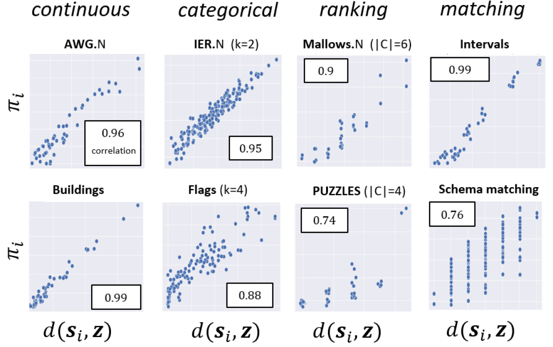
Figure 11: Each scatterplot presents all workers in a single instance, with their disparity $\pi_{i}$ vs. their real error $d(\bm{s}_{i},\bm{z})$.

Fig. 3 in the main text shows the correlation of workers’ empirical disparity $\pi_{i}$ with their distance from the ground truth.

Fig. 11 is the same figure, but now specifying the dataset we used, and also synthetic distributions.

The two datasets not already described above are schemaMatching, where users were asked to align the attributes of two database schemata (Shraga, Gal, and Roitman 2018); and Intervals which is a synthetic dataset we constructed where $\bm{z}$ is a set of intervals, and each report $\bm{s}_{i}$ is a noisy version of it. Both use the Jaccard distance metric.

Additional Results

Here we add tables and figures showing performance of all algorithms on the same datasets under different numbers of workers and questions.

Real-valued data, $m=15,n=30$
Real-valued		CRH	CATD	GTM	KDE	EXP	TOP2	MAS	P-TDD	P-TDAK	iP-TD
SYN.N	$-$	-33%	-61%	-27%	+7%	-12%	-22%	+52%	-38%	-70%	-43%
BUILD	$-$	-19%	-20%	-22%	-34%	-29%	+68%	-25%	-21%	-25%	-33%
TRI1	$-$	-18%	-7%	-18%	+8%	-27%	+68%	+27%	-18%	-8%	-21%
TRI2	$-$	-11%	-22%	-8%	-19%	-17%	-26%	+2%	-11%	-8%	-17%
Real-valued data, $m=50,n=10$
Real-valued		CRH	CATD	GTM	KDE	EXP	TOP2	MAS	P-TDD	P-TDAK	iP-TD
SYN.N	$-$	-37%	-32%	-38%	+32%	-15%	-14%	+77%	-34%	-62%	-40%
TRI1	$-$	-31%	-5%	-32%	+1%	-28%	+26%	+78%	-29%	-10%	-30%
TRI2	$-$	-14%	-10%	-12%	-0%	-19%	-11%	+21%	-11%	-10%	-17%
EMO	$-$	+4%	+47%	+6%	+76%	+20%	+66%	+15%	+4%	+12%	+7%

Table 5: $m=50,n=10$

Ranking	v. rule	D-TD	EXP	TOP2	MAS	P-TDD	iP-TD
SYN.HS	Veto	+2%	-5%	-0%	-9%	-6%	-7%
SYN.N	Veto	+5%	-0%	+51%	-3%	-9%	-10%
BUILD	Veto	+1%	+6%	+51%	-5%	-7%	-6%
DOTS3	Veto	+3%	-5%	+10%	-8%	-10%	-14%
DOTS5	Veto	+5%	-8%	+16%	-7%	-14%	-17%
DOTS7	Veto	+4%	-9%	+52%	-5%	-16%	-21%
DOTS9	Veto	+10%	-7%	+48%	-7%	-18%	-23%
PUZZ5	Veto	+4%	-14%	+40%	-16%	-22%	-29%
PUZZ7	Veto	+7%	-4%	+59%	-11%	-21%	-22%
PUZZ9	Veto	+3%	-7%	+28%	-15%	-15%	-19%
PUZZ11	Veto	+6%	-3%	+16%	-6%	-10%	-13%
SYN.N	Best worker	-12%	-21%	-72%	-87%	-89%	-89%
BUILD	Best worker	-9%	-20%	-52%	-51%	-57%	-57%
DOTS3	Best worker	-19%	-9%	-43%	-53%	-59%	-59%
PUZZ5	Best worker	-25%	-37%	-92%	-94%	-93%	-94%
SYN.N	Kemeny-Young	-2%	+4%	+176%	+1%	-8%	-8%
BUILD	Kemeny-Young	-1%	-1%	+12%	-4%	-1%	-1%
DOTS3	Kemeny-Young	+1%	+2%	+37%	-2%	-4%	-2%
PUZZ5	Kemeny-Young	-2%	+1%	+6%	+23%	-23%	-27%

Table 6: Results (RI) on ranking data, $n=10$, additional voting rules.

Ranking	v. rule	D-TD	EXP	TOP2	MAS	P-TDD	iP-TD
SYN.HS	Borda	-20%	-1%	-58%	-43%	-7%	-20%
SYN.N	Borda	-10%	-2%	+91%	-27%	-12%	-17%
BUILD	Borda	+2%	+0%	+0%	+0%	+0%	+0%
DOTS3	Borda	-0%	+2%	+44%	+2%	-2%	+1%
DOTS5	Borda	-2%	-2%	+60%	+25%	-8%	-10%
DOTS7	Borda	+0%	+6%	+127%	+18%	-12%	-11%
DOTS9	Borda	-5%	+3%	+86%	-22%	-23%	-30%
PUZZ5	Borda	+1%	-7%	-36%	-40%	-29%	-44%
PUZZ7	Borda	+5%	+18%	+139%	+18%	-13%	-2%
PUZZ9	Borda	+1%	-6%	+28%	-9%	-13%	-20%
PUZZ11	Borda	-0%	+3%	+23%	-20%	-4%	-5%
SYN.N	Plurality	+3%	-8%	+171%	-11%	-12%	-14%
BUILD	Plurality	-2%	-0%	+61%	-13%	-6%	-6%
DOTS3	Plurality	+6%	+1%	+91%	-5%	-5%	-6%
PUZZ5	Plurality	+6%	-16%	+126%	-23%	-27%	-37%
SYN.N	Copeland	-6%	-9%	+107%	-18%	-31%	-31%
BUILD	Copeland	+2%	-0%	-0%	+1%	-1%	-0%
DOTS3	Copeland	-1%	-6%	+10%	-18%	-23%	-21%
PUZZ5	Copeland	-1%	-20%	-22%	-41%	-44%	-46%

Table 7: Results (RI) on ranking data, $n=30$.

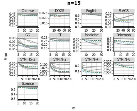
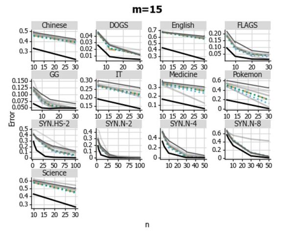
Figure 12: Error on all categorical datasets.

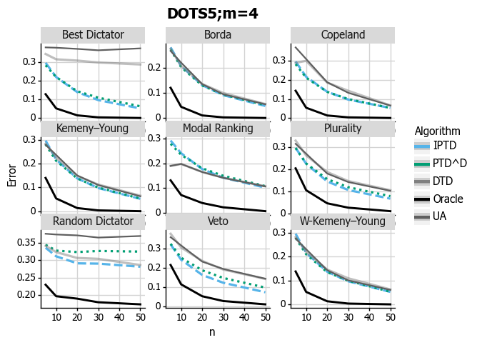
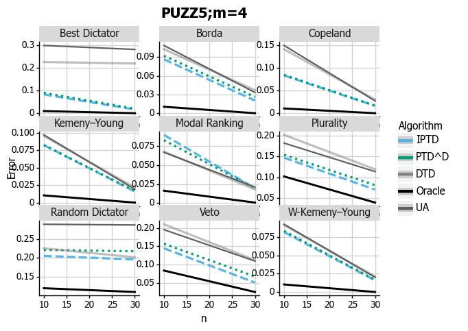
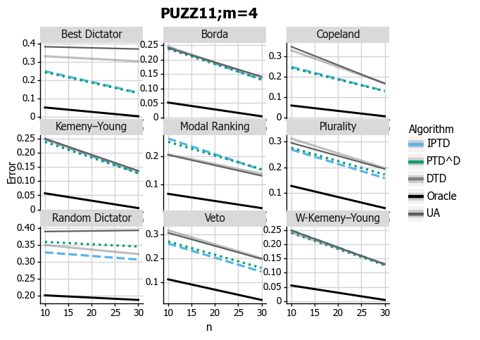
Figure 13: Error on more ranking datasets, under all nine voting rules, 4 candidates.

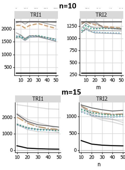
Figure 14: Error on the real-valued TRI datasets.

References

- Aitkin (1935) Aitkin, A. 1935. On least squares and linear combination of observations. Proceedings of the RSE, 55: 42–48.
- Aydin et al. (2014) Aydin, B. I.; Yilmaz, Y. S.; Li, Y.; Li, Q.; Gao, J.; and Demirbas, M. 2014. Crowdsourcing for multiple-choice question answering. In Twenty-Sixth IAAI Conference.
- Ben-Yashar and Paroush (2001) Ben-Yashar, R.; and Paroush, J. 2001. Optimal decision rules for fixed-size committees in polychotomous choice situations. Social Choice and Welfare, 18(4): 737–746.
- Braylan and Lease (2020) Braylan, A.; and Lease, M. 2020. Modeling and Aggregation of Complex Annotations via Annotation Distances. In Proceedings of The Web Conference 2020, 1807–1818.
- Caragiannis, Procaccia, and Shah (2013) Caragiannis, I.; Procaccia, A. D.; and Shah, N. 2013. When do noisy votes reveal the truth? In EC’13, 143–160. ACM.
- Carter, Morris, and Blashfield (1989) Carter, R. L.; Morris, R.; and Blashfield, R. K. 1989. On the partitioning of squared Euclidean distance and its applications in cluster analysis. Psychometrika, 54(1): 9–23.
- Condorcet (1785) Condorcet, M. J. 1785. Essai sur l’application de l’analyse à la probabilité des décisions rendues à la pluralité des voix. Trans. lain McLean and Fiona Hewitt. Paris.
- Dalvi et al. (2013) Dalvi, N.; Dasgupta, A.; Kumar, R.; and Rastogi, V. 2013. Aggregating crowdsourced binary ratings. In WWW’13, 285–294.
- Dawid and Skene (1979) Dawid, A. P.; and Skene, A. M. 1979. Maximum likelihood estimation of observer error-rates using the EM algorithm. Journal of the Royal Statistical Society: Series C (Applied Statistics), 28(1): 20–28.
- Deng et al. (2014) Deng, J.; Russakovsky, O.; Krause, J.; Bernstein, M. S.; Berg, A.; and Fei-Fei, L. 2014. Scalable multi-label annotation. In SIGCHI’14, 3099–3102. ACM.
- Diebold (1998) Diebold, F. X. 1998. Elements of forecasting. South-Western College Pub.
- Gadiraju et al. (2017) Gadiraju, U.; Fetahu, B.; Kawase, R.; Siehndel, P.; and Dietze, S. 2017. Using worker self-assessments for competence-based pre-selection in crowdsourcing microtasks. TOCHI, 24(4): 1–26.
- Gao and Zhou (2013) Gao, C.; and Zhou, D. 2013. Minimax optimal convergence rates for estimating ground truth from crowdsourced labels. arXiv preprint arXiv:1310.5764.
- Grofman, Owen, and Feld (1983) Grofman, B.; Owen, G.; and Feld, S. L. 1983. Thirteen theorems in search of the truth. Theory and Decision, 15(3): 261–278.
- Hart et al. (2018) Hart, Y.; Dillon, M. R.; Marantan, A.; Cardenas, A. L.; Spelke, E.; and Mahadevan, L. 2018. The statistical shape of geometric reasoning. Scientific reports, 8(1): 12906.
- Huang and Fu (2013) Huang, S.-W.; and Fu, W.-T. 2013. Enhancing reliability using peer consistency evaluation in human computation. In CSCW, 639–648. ACM.
- Karger, Oh, and Shah (2011) Karger, D. R.; Oh, S.; and Shah, D. 2011. Iterative learning for reliable crowdsourcing systems. In NeurIPS’11, 1953–1961.
- Kawase, Kuroki, and Miyauchi (2019) Kawase, Y.; Kuroki, Y.; and Miyauchi, A. 2019. Graph mining meets crowdsourcing: Extracting experts for answer aggregation. In IJCAI’19.
- Kobayashi (2018) Kobayashi, H. 2018. Frustratingly easy model ensemble for abstractive summarization. In EMNLP’18, 4165–4176.
- Kurvers et al. (2019) Kurvers, R. H.; Herzog, S. M.; Hertwig, R.; Krause, J.; Moussaid, M.; Argenziano, G.; Zalaudek, I.; Carney, P. A.; and Wolf, M. 2019. How to detect high-performing individuals and groups: Decision similarity predicts accuracy. Science advances, 5(11): eaaw9011.
- Li, Baba, and Kashima (2018) Li, J.; Baba, Y.; and Kashima, H. 2018. Incorporating worker similarity for label aggregation in crowdsourcing. In International Conference on Artificial Neural Networks, 596–606. Springer.
- Li et al. (2014a) Li, Q.; Li, Y.; Gao, J.; Su, L.; Zhao, B.; Demirbas, M.; Fan, W.; and Han, J. 2014a. A confidence-aware approach for truth discovery on long-tail data. Proceedings of the VLDB Endowment, 8(4): 425–436.
- Li et al. (2014b) Li, Q.; Li, Y.; Gao, J.; Zhao, B.; Fan, W.; and Han, J. 2014b. Resolving conflicts in heterogeneous data by truth discovery and source reliability estimation. In SIGMOD’14.
- Li et al. (2012) Li, X.; Dong, X. L.; Lyons, K.; Meng, W.; and Srivastava, D. 2012. Truth finding on the deep web: is the problem solved? Proceedings of the VLDB Endowment, 6(2): 97–108.
- Li et al. (2016) Li, Y.; Gao, J.; Meng, C.; Li, Q.; Su, L.; Zhao, B.; Fan, W.; and Han, J. 2016. A survey on truth discovery. ACM SIGKDD Explorations Newsletter, 17(2): 1–16.
- Mandal, Radanovic, and Parkes (2020) Mandal, D.; Radanovic, G.; and Parkes, D. C. 2020. The Effectiveness of Peer Prediction in Long-Term Forecasting. In AAAI’20.
- Mao, Procaccia, and Chen (2013) Mao, A.; Procaccia, A. D.; and Chen, Y. 2013. Better human computation through principled voting. In AAAI’13.
- McLaughlin (2014) McLaughlin, E. 2014. Image Overload: Help us sort it all out, NASA requests. CNN.com. Retrieved at 18/9/2014.
- Parisi et al. (2014) Parisi, F.; Strino, F.; Nadler, B.; and Kluger, Y. 2014. Ranking and combining multiple predictors without labeled data. PNAS, 111(4): 1253–1258.
- Prelec, Seung, and McCoy (2017) Prelec, D.; Seung, H. S.; and McCoy, J. 2017. A solution to the single-question crowd wisdom problem. Nature, 541(7638): 532.
- Shah and Zhou (2015) Shah, N. B.; and Zhou, D. 2015. Double or nothing: Multiplicative incentive mechanisms for crowdsourcing. In NeurIPS’15, 1–9.
- Shraga, Gal, and Roitman (2018) Shraga, R.; Gal, A.; and Roitman, H. 2018. What Type of a Matcher Are You? Coordination of Human and Algorithmic Matchers. In Proceedings of the HILL’19 Workshop, 1–7.
- Snow et al. (2008) Snow, R.; O’connor, B.; Jurafsky, D.; and Ng, A. Y. 2008. Cheap and fast–but is it good? evaluating non-expert annotations for natural language tasks. In Proceedings of the 2008 conference on empirical methods in natural language processing, 254–263.
- Spiers et al. (2021) Spiers, H.; Songhurst, H.; Nightingale, L.; De Folter, J.; Community, Z. V.; Hutchings, R.; Peddie, C. J.; Weston, A.; Strange, A.; Hindmarsh, S.; et al. 2021. Deep learning for automatic segmentation of the nuclear envelope in electron microscopy data, trained with volunteer segmentations. Traffic, 22(7): 240–253.
- Von Ahn and Dabbish (2008) Von Ahn, L.; and Dabbish, L. 2008. Designing games with a purpose. Communications of the ACM, 51(8): 58–67.
- Vuurens, de Vries, and Eickhoff (2011) Vuurens, J.; de Vries, A. P.; and Eickhoff, C. 2011. How much spam can you take? an analysis of crowdsourcing results to increase accuracy. In ACM SIGIR Workshop on CIR’ 11, 21–26.
- Wais et al. (2010) Wais, P.; Lingamneni, S.; Cook, D.; Fennell, J.; Goldenberg, B.; Lubarov, D.; Marin, D.; and Simons, H. 2010. Towards building a high-quality workforce with mechanical turk. NeurIPS workshop, 1–5.
- Wan et al. (2016) Wan, M.; Chen, X.; Kaplan, L.; Han, J.; Gao, J.; and Zhao, B. 2016. From truth discovery to trustworthy opinion discovery: An uncertainty-aware quantitative modeling approach. In SIGKDD’16, 1885–1894.
- Witkowski et al. (2013) Witkowski, J.; Bachrach, Y.; Key, P.; and Parkes, D. 2013. Dwelling on the negative: Incentivizing effort in peer prediction. In Proceedings of the AAAI Conference on Human Computation and Crowdsourcing, volume 1.
- Wu et al. (2016) Wu, Y.; Schuster, M.; Chen, Z.; Le, Q. V.; Norouzi, M.; Macherey, W.; Krikun, M.; Cao, Y.; Gao, Q.; Macherey, K.; et al. 2016. Google’s neural machine translation system: Bridging the gap between human and machine translation. arXiv preprint arXiv:1609.08144.
- Xiao et al. (2016) Xiao, H.; Gao, J.; Wang, Z.; Wang, S.; Su, L.; and Liu, H. 2016. A truth discovery approach with theoretical guarantee. In SIGKDD’16, 1925–1934.
- Yin and Tan (2011) Yin, X.; and Tan, W. 2011. Semi-supervised truth discovery. In WWW’11, 217–226.
- Zhang et al. (2016) Zhang, Y.; Chen, X.; Zhou, D.; and Jordan, M. I. 2016. Spectral methods meet EM: A provably optimal algorithm for crowdsourcing. JMLR, 17(1): 3537–3580.
- Zhao and Han (2012) Zhao, B.; and Han, J. 2012. A probabilistic model for estimating real-valued truth from conflicting sources. Proc. of QDB, 1817.