Variational Autoencoders for Sparse and Overdispersed Discrete Data

Abstract

Many applications, such as text modelling, high-throughput sequencing, and recommender systems, require analysing sparse, high-dimensional, and overdispersed discrete (count-valued or binary) data. Although probabilistic matrix factorisation and linear/nonlinear latent factor models have enjoyed great success in modelling such data, many existing models may have inferior modelling performance due to the insufficient capability of modelling overdispersion in count-valued data and model misspecification in general. In this paper, we comprehensively study these issues and propose a variational autoencoder based framework that generates discrete data via negative-binomial distribution. We also examine the model’s ability to capture properties, such as self- and cross-excitations in discrete data, which is critical for modelling overdispersion. We conduct extensive experiments on three important problems from discrete data analysis: text analysis, collaborative filtering, and multi-label learning. Compared with several state-of-the-art baselines, the proposed models achieve significantly better performance on the above problems.

1 Introduction

Discrete data are ubiquitous in many applications. For example, in text analysis, a collection of documents can be represented as a word-document count matrix with the bag-of-words assumption; in recommender systems, users’ shopping history can be represented as a binary (or count) item-user matrix, with each entry indicating whether or not a user has bought an item (or its purchase count); in extreme multi-label learning problems, data samples can be tagged with a large set of labels, presented by a binary label matrix. Such kinds of data are often characterised by high-dimensionality and extreme sparsity.

With the ability to handle high-dimensional and sparse matrices, Probabilistic Matrix Factorisation (PMF) [27] has been a key method of choice for such problems. PMF assumes data is generated from a suitable probability distribution, parameterised by low-dimensional latent factors. When it comes to discrete data, Latent Dirichlet Allocation (LDA) [2] and Poisson Factor Analysis (PFA) [6, 44] are the two representative models that generate data samples using the multinomial and Poisson distributions, respectively. Originally, LDA and PFA can be seen as single-layer models, whose modelling expressiveness may be limited. Therefore, extensive research has been devoted to extending them with hierarchical Bayesian priors [3, 28, 13, 45]. However, increasing model complexity with hierarchical priors can also complicate inference, and lack of scalability hinders their usefulness in analysing large-scale data. The recent success of deep generative models such as Variational Autoencoders (VAEs) [20, 30] on modelling real-valued data such as images has motivated machine learning practitioners to adapt VAEs to dealing with discrete data as done in recent works [25, 26, 21, 22]. Instead of using the Gaussian distribution as the data distribution for real-valued data, the multinomial distribution has been used for discrete data [25, 21, 22]. Following Liang et al. [22], we refer to these VAE-based models as “MultiVAE” (Multi for multinomial). MultiVAE can be viewed as a deep nonlinear PMF model, where the nonlinearity is introduced by the deep neural networks in the decoder. Compared with conventional hierarchical Bayesian models, MultiVAE increases its modelling capacity without sacrificing the scalability, because of the use of amortized variational inference (AVI) [30].

Nevertheless, the use of the multinomial data distribution in existing VAE models such as MultiVAE can lead to inferior modelling performance on discrete data due to: 1) insufficient capability of modelling overdispersion in count-valued data, and 2) model misspecification in binary data. Specifically, overdispersion (i.e., variance larger than the mean) describes the phenomenon that the data variability is large, which is a key property for large-scale count-valued data. For example, overdispersion in text data can behave as word burstiness [9, 23, 11, 5], which happens as if a word is seen in a document, it may excite both itself and related ones. Burstiness can cause overdispersion in text data because a document usually has a few bursty words occurring multiple times while other words only show up once or never, resulting in high variance in bag-of-word matrices. Shown in Zhou [43], the deep-seated causes of insufficient capability of modelling overdispersion in existing PMF models with Poisson or multinomial are due to their limited ability of handling self- and cross-excitation [43]. Specifically, in the text data example, self-excitation captures the effect that if a word occurs in a document, it is likely to occur more times in the same document. On the other hand, cross-excitation models the effect that if a word such as “puppy” occurs, it will likely to excite the occurrences of related words such as “dog.” It can be shown that existing PMF models with Poisson/multinomial do not distinguish between self- and cross-excitation and usually assume that data are independently generated. Moreover, besides count-valued data, binary-valued observations are also prevalent in many applications, such as in collaborative filtering and graph analysis. It may not be proper to directly apply multinomial or Poisson to binary data, which is a common misspecification in many existing models. This is because multinomial and Poisson may assign more than one count to one position, ignoring the fact that the data are binary. The misspecification could result in inferior modelling performance [42].

In this paper, we show the above two issues on modelling discrete data can be addressed in a principled manner using the negative-binomial (NB) distribution as the data distribution in a deep-structured PMF model. Specifically, in Section 2, we analytically demonstrate that using NB as the data likelihood in PMFs can explicitly capture self-excitation and using deep structures can provide more model capacity for capturing cross-excitation. Therefore, a deep PMF with NB is able to better handle overdispersion by sufficiently capturing both kinds of excitations. On the other hand, the usage of NB instead of multinomial enables us to develop a link function between the Bernoulli and negative-binomial distributions, which gives us the ability to handle binary data with superior modelling performance. Beside the in-depth analytical study, we propose a deep PMF model called Negative-Binomial Variational AutoEncoder (NBVAE for short), a VAE-based framework generating data with a negative-binomial distribution. Extensive experiments have been conducted on three important problems of discrete data analysis: text analysis on bag-of-words data, collaborative filtering on binary data, and multi-label learning. Compared with several state-of-the-art baselines, NBVAE achieves significantly better performance on the above problems.

2 Analytical study and model details

In this section, we start with the introduction of our proposed NBVAE model for count-valued data, and then give a detailed analysis on how self- and cross-excitations are captured in different models and why NBVAE is capable of better handling them. Finally, we describe the variants of NBVAE for modelling binary data and for multi-label learning, respectively.

2.1 Negative-binomial variational autoencoder (NBVAE)

Like the standard VAE model, NBVAE consists of two major components: the decoder for the generative process and the encoder for the inference process. Here we focus on the generative process and discuss the inference procedure in Section 3. Without loss of generality, we present our model in the case of bag-of-word data for a text corpus, but the model can generally work with any kind of count-valued matrices. Suppose the bag-of-word data are stored in a $V$ by $N$ count matrix $\mathbf{Y}\in\mathbb{N}^{V\times N}=[\boldsymbol{y}_{1},\cdots,\boldsymbol{y}_{N}]$, where $\mathbb{N}=\{0,1,2,\cdots\}$ and $V$ and $N$ are the number of documents and the size of the vocabulary, respectively. To generate the occurrences of the words for the $j^{\text{th}}$ ($j\in\{1,\cdots N\}$) document, $\boldsymbol{y}_{j}\in\mathbb{N}^{V}$, we draw a $K$ dimensional latent representation $\boldsymbol{z}_{j}\in\mathbb{R}^{K}$ from a standard multivariate normal prior. After that, $\boldsymbol{y}_{j}$ is drawn from a (multivariate) negative-binomial distribution with $\boldsymbol{r}_{j}\in\mathbb{R}_{+}^{V}$ ($\mathbb{R}_{+}=\{x:x\geq 0\}$) and $\boldsymbol{p}_{j}\in(0,1)^{V}$ as the parameters. Moreover, $\boldsymbol{r}_{j}$ and $\boldsymbol{p}_{j}$ are obtained by transforming $\boldsymbol{z}_{j}$ from two nonlinear functions, $f_{\theta^{r}}(\boldsymbol{\cdot})$ and $f_{\theta^{p}}(\boldsymbol{\cdot})$, parameterised by $\theta^{r}$ and $\theta^{p}$, respectively. The above generative process of $\operatorname{p}(\boldsymbol{y}_{j}\nonscript\;|\nonscript\;\boldsymbol{z}_{j})$ can be formulated as follows: +rCl+x* z_j ∼N(0,I_K), r_j = exp(f_θ^r(z_j)), p_j = 1/(1 + exp(-f_θ^p(z_j)), y_j ∼NB(r_j, p_j).

In the above model, the output of $f_{\theta^{p}}(\boldsymbol{\cdot})$, $\boldsymbol{p}_{j}$, is a $V$ dimensional vector. Alternatively, if we set the output of $f_{\theta^{p}}(\boldsymbol{\cdot})$ a single number $p_{j}\in(0,1)$ specific to document $j$, according to Zhou [43, Theorem 1], we can derive an alternative representation of NBVAE: +rCl+x* &z_j ∼N(0,I_K), r_j = exp(f_θ^r(z_j)), p_j = 1/(1 + exp(-f_θ^p(z_j)),
y_⋅j ∼NB(r_⋅j, p_j), y_j ∼DirMulti(y_⋅j, r_j), where “DirMulti” stands for the Dirichlet-multinomial distribution, $y_{\boldsymbol{\cdot}j}=\sum_{v}^{V}y_{vj}$ is the total number of words of document $j$, and $r_{\boldsymbol{\cdot}j}=\sum_{v}^{V}r_{vj}$. Accordingly, we refer this representation of NBVAE to as NBVAE${}_{\text{dm}}$ (dm for Dirichlet-multinomial). Note that NBVAE${}_{\text{dm}}$ can also be viewed as a deep nonlinear generalization of models based on Dirichlet-multinomial to capture word burstiness [11, 5]. Compared with NBVAE, when doing inference for NBVAE${}_{\text{dm}}$, we can treat $y_{\boldsymbol{\cdot}j}$, i.e., the total number of words as an observed variable.

2.2 How NBVAE captures self- and cross-excitations

We now compare NBVAE and other PMF models in terms of their ability in capturing self- and cross-excitations in count-valued data. For easy comparison, we present the related PMF models with a unified framework. Without loss of generality, we demonstrate the framework in the case of bag-of-word text data, where the $i^{\text{th}}$ word’s type in document $j$ is $w^{i}_{j}\in\{1,\cdots,V\}$ and the occurrence of $v$ in document $j$ is $y_{vj}$. The first thing we are interested in is the data distribution that generates the word occurrences of document $j$. Specifically, we can generate $\{w^{i}_{j}\}_{i=1}^{y_{\boldsymbol{\cdot}j}}$ from $\operatorname{p}(w^{i}_{j}=v\nonscript\;|\nonscript\;\boldsymbol{l}_{j})\propto l_{vj}/l_{\boldsymbol{\cdot}j}$ where $\boldsymbol{l}_{j}\in\mathbb{R}_{+}^{V}$ is the model parameter. After all the word types are generated, we can count the occurrences of different types of words by $y_{vj}=\sum_{i}^{y_{\boldsymbol{\cdot}j}}\textbf{1}(w^{i}_{j}=v)$, where $\textbf{1}(\boldsymbol{\cdot})$ is the indicator function. Alternatively, we can directly generate $\boldsymbol{y}_{j}$ from $\operatorname{p}(\boldsymbol{y}_{j}\nonscript\;|\nonscript\;\boldsymbol{l}_{j})$. As shown later, for PMF models, $\boldsymbol{l}_{j}$ explicitly or implicitly takes a factorised form. Moreover, we are more interested in the predictive distribution of a word, $w^{i}_{j}$, conditioned on the other words’ occurrences in the corpus, $\mathbf{Y}^{-ij}$, which can be presented as follows: +rCl+x* p(w^i_j = v | Y^-ij ) &∝ ∫p(w^i_j = v | l’_j ) p(l’_j | Y^-ij ) d l’_j = E_p(l’_j | Y^-ij )[p(w^i_j = v | l’_j )], where $\boldsymbol{l}^{\prime}_{j}$ is the predictive rate computed with the parameters obtained from the posterior.

Now we reformulate the models related to NBVAE into the above framework, including Poisson Factor Analysis (PFA) [6, 44], Latent Dirichlet Allocation (LDA) [2], MultiVAE [25, 21, 22], and Negative-Binomial Factor Analysis (NBFA) [43], as follows:

PFA: It is obvious that PFA directly fits into this framework, where $\operatorname{p}(\boldsymbol{y}_{j}\nonscript\;|\nonscript\;\boldsymbol{l}_{j})$ is the Poisson distribution and $\boldsymbol{l}_{j}=\mathbf{\Phi}\boldsymbol{\theta}_{j}$. Here $\mathbf{\Phi}\in\mathbb{R}_{+}^{V\times K}=[\boldsymbol{\phi}_{1},\cdots,\boldsymbol{\phi}_{K}]$ is the factor loading matrix and $\mathbf{\Theta}\in\mathbb{R}_{+}^{K\times N}=[\boldsymbol{\theta}_{1},\cdots,\boldsymbol{\theta}_{N}]$ is the factor score matrix. Their linear combinations determine the probability of the occurrence of $v$ in document $j$.

LDA: Originally, LDA explicitly assigns a topic $z^{i}_{j}\in\{1,\cdots,K\}$ to $w^{i}_{j}$, with the following process: $z^{i}_{j}\sim\text{Cat}(\boldsymbol{\theta}_{j}/\theta_{\boldsymbol{\cdot}j})$ and $w^{i}_{j}\sim\text{Cat}(\boldsymbol{\phi}_{z_{ij}})$, where $\theta_{\boldsymbol{\cdot}j}=\sum_{k}^{K}\theta_{kj}$ and “Cat” is the categorical distribution. By collapsing all the topics, we can derive an equivalent representation of LDA, in line with the general framework: $\boldsymbol{y}_{j}\sim\text{Multi}(y_{\boldsymbol{\cdot}j},\boldsymbol{l}_{j})$, where $\boldsymbol{l}_{j}=\mathbf{\Phi}\boldsymbol{\theta}_{j}/\theta_{\boldsymbol{\cdot}j}$.

MultiVAE: MultiVAE generates data from a multinomial distribution, whose parameters are constructed by the decoder: $\boldsymbol{y}_{j}\sim\text{Multi}(y_{\boldsymbol{\cdot}j},\boldsymbol{l}_{j})$, where $\boldsymbol{l}_{j}=\text{softmax}(f_{\theta}(\boldsymbol{z}_{j}))$. As shown in Krishnan et al. [21], MultiVAE can be viewed as a nonlinear PMF model.

NBFA: NBFA uses a negative-binomial distribution as the data distribution, the generative process of which can be represented as: $\boldsymbol{y}_{j}\sim\text{NB}(\boldsymbol{l}_{j},p_{j})$, where $\boldsymbol{l}_{j}=\mathbf{\Phi}\boldsymbol{\theta}_{j}$.

Table 1: Comparison of the data distributions, model parameters, predictive rates, and posteriors. $\operatorname{q}(\boldsymbol{\cdot})$ denotes the encoder in VAE models, which will be introduced in Section 3.

Model	Data distribution	Model parameter	Predictive rate	Posterior
PFA	$\boldsymbol{y}_{j}\sim\text{Poisson}(\boldsymbol{l}_{j})$	$\boldsymbol{l}_{j}=\mathbf{\Phi}\boldsymbol{\theta}_{j}$	$l^{\prime}_{vj}\propto\sum_{k}^{K}\phi_{vk}\theta_{kj}$	$\mathbf{\Phi},\boldsymbol{\theta}_{j}\sim\operatorname{p}(\mathbf{\Phi},\boldsymbol{\theta}_{j}\nonscript\;|\nonscript\;\mathbf{Y}^{-ij})$
LDA	$\boldsymbol{y}_{j}\sim\text{Multi}(y_{\boldsymbol{\cdot}j},\boldsymbol{l}_{j})$	$\boldsymbol{l}_{j}=\mathbf{\Phi}\boldsymbol{\theta}_{j}/\theta_{\boldsymbol{\cdot}j}$	$l^{\prime}_{vj}\propto\sum_{k}^{K}\phi_{vk}\theta_{kj}/\theta_{\boldsymbol{\cdot}j}$	$\mathbf{\Phi},\boldsymbol{\theta}_{j}\sim\operatorname{p}(\mathbf{\Phi},\boldsymbol{\theta}_{j}\nonscript\;|\nonscript\;\mathbf{Y}^{-ij})$
MultiVAE	$\boldsymbol{y}_{j}\sim\text{Multi}(y_{\boldsymbol{\cdot}j},\boldsymbol{l}_{j})$	$\boldsymbol{l}_{j}=\text{softmax}(f_{\theta}(\boldsymbol{z}_{j}))$	$l^{\prime}_{vj}\propto\text{softmax}(f_{\theta}(\boldsymbol{z}_{j}))_{v}$	$\boldsymbol{z}_{j}\sim\operatorname{q}(\boldsymbol{z}_{j}\nonscript\;|\nonscript\;\mathbf{Y}^{-ij})$
NBFA	$\boldsymbol{y}_{j}\sim\text{NB}(\boldsymbol{l}_{j},p_{j})$	$\boldsymbol{l}_{j}=\mathbf{\Phi}\boldsymbol{\theta}_{j}$	$l^{\prime}_{vj}\propto(y_{vj}^{-i}+\sum_{k}^{K}\phi_{vk}\theta_{kj})p_{j}$	$\mathbf{\Phi},\boldsymbol{\theta}_{j},p_{j}\sim\operatorname{p}(\mathbf{\Phi},\boldsymbol{\theta}_{j},p_{j}\nonscript\;|\nonscript\;\mathbf{Y}^{-ij})$
NBVAE	$\boldsymbol{y}_{j}\sim\text{NB}(\boldsymbol{r}_{j},\boldsymbol{p}_{j})$	$\boldsymbol{r}_{j}=\text{exp}\left(f_{\theta^{r}}(\boldsymbol{z}_{j})\right)$ $\boldsymbol{p}_{j}=1/(1+\text{exp}\left(-f_{\theta^{p}}(\boldsymbol{z}_{j}\right))$	$l^{\prime}_{vj}\propto\frac{y_{vj}^{-i}+\text{exp}\left(f_{\theta^{r}}(\boldsymbol{z}_{j})\right)_{v}}{\left(1+\text{exp}\left(-f_{\theta^{p}}(\boldsymbol{z}_{j}\right)\right)_{v}}$	$\boldsymbol{z}_{j}\sim\operatorname{q}(\boldsymbol{z}_{j}\nonscript\;|\nonscript\;\mathbf{Y}^{-ij})$
NBVAE${}_{\text{dm}}$	$\boldsymbol{y}_{j}\sim\text{DirMulti}\left(y_{\boldsymbol{\cdot}j},\boldsymbol{r}_{j}\right)$	$\boldsymbol{r}_{j}=\text{exp}\left(f_{\theta^{r}}(\boldsymbol{z}_{j})\right)$ $p_{j}=1/(1+\text{exp}\left(-f_{\theta^{p}}(\boldsymbol{z}_{j}\right))$	$l^{\prime}_{vj}\propto y_{vj}^{-i}+\text{exp}\left(f_{\theta^{r}}(\boldsymbol{z}_{j})\right)_{v}$	$\boldsymbol{z}_{j}\sim\operatorname{q}(\boldsymbol{z}_{j}\nonscript\;|\nonscript\;\mathbf{Y}^{-ij})$

Table 2: How different models capture self- and cross-excitation

Model	Self-excitation	Cross-excitation
PFA	Single-layer structure
LDA	Single-layer structure
MultiVAE	Multi-layer neural networks
NBFA	$y_{vj}^{-i}$	Single-layer structure
NBVAE NBVAE${}_{\text{dm}}$	$y_{vj}^{-i}$	Multi-layer neural networks

The above comparisons on the data distributions and predictive distributions of those models are shown in Table 1. In particular, we can show a model’s capacity of capturing self- and cross-excitations by analysing its predictive distribution. Note that $y_{vj}^{-i}$ denotes the number of $v$’s occurrences in document $j$ excluding the $i^{\text{th}}$ word. If we compare PFA, LDA, MultiVAE V.S. NBFA, NBVAE, NBVAE${}_{\text{dm}}$, it can be seen that the latter three models with NB as their data distributions explicitly capture self-excitation via the term $y_{vj}^{-i}$ in the predictive distributions. Specifically, if $v$ appears more in document $j$, $y_{vj}^{-i}$ will be larger, leading to larger probability that $v$ shows up again. That is to say, the latter three models capture word burstiness directly with $y_{vj}^{-i}$. However, PFA, LDA, and MultiVAE cannot capture self-excitation directly because they predict a word purely based on the interactions of the latent representations and pay less attention to the existing word frequencies. Therefore, even with deep structures, their potential of modelling self-excitation is still limited. Moreover, for the models with NB, i.e., NBVAE and NBFA, as self-excitation is explicitly captured by $y_{vj}^{-i}$, the interactions of the latent factors are only responsible for cross-excitation. Specifically, NBFA applies a single-layer linear combination of the latent representations, i.e., $\sum_{k}^{K}\phi_{vk}\theta_{kj}$, while NBVAE can be viewed as a deep extension of NBFA, using a deep neural network to conduct multi-layer nonlinear combinations of the latent representations, i.e, $r_{vj}=\text{exp}\left(f_{\theta^{r}}(\boldsymbol{z}_{j})\right)_{v}$ and $p_{vj}=1/(1+\text{exp}\left(-f_{\theta^{p}}(\boldsymbol{z}_{j}\right))_{v}$. Therefore, NBVAE enjoys richer modelling capacity than NBFA on capturing cross-excitation. Finally, we summarise our analysis on how self- and cross-excitations are captured in related models in Table 2.

2.3 NBVAE for binary data

In many problems, discrete data are binary-valued. For example, suppose the binary matrix $\mathbf{Y}\in\{0,1\}^{V\times N}$ stores the buying history of $N$ users on $V$ items, where $y_{vj}=1$ indicates that user $j$ has brought item $v$. Precious models like MultiVAE [21, 22] treat such binary data as counts, which is a model misspecification that is likely to result in inferior performance. To better model binary data, we develop a simple yet effective method that links NBVAE and the Bernoulli distribution. Specifically, inspired by the link function used in Zhou [42], we first generate a latent discrete intensity vector, $\boldsymbol{m}_{j}\in\mathbb{N}^{V}$, from the generative process of NBVAE, where $m_{vj}$ can be viewed as the interest of user $j$ on item $v$. Next, we generate the binary buying history of user $j$ by thresholding the discrete intensity vector at one, as follows: +rCl+x* m_j ∼NBVAE(z_j),   y_j = 1(m_j ≥1). As $\boldsymbol{m}_{j}$ is drawn from NB, we do not have to explicitly generate it. Instead, if we marginalise it out, we can get the following data likelihood: $\boldsymbol{y}_{j}\sim\text{Bernoulli}\left(1-(1-\boldsymbol{p}_{j})^{\boldsymbol{r}_{j}}\right),$ where $\boldsymbol{r}_{j}$ and $\boldsymbol{p}_{j}$ have the same construction of the original NBVAE. Here we refer to this extension of NBVAE as NBVAE${}_{\text{b}}$ (b for binary). Given the fact that the NB distribution is a gamma mixed Poisson distribution, the elements of $\boldsymbol{m}_{j}$ can be viewed to be individually generated from a Poisson distribution. In contrast, a vector’s elements are jointly generated from multinomial in MutiVAE and Dirichlet-multinomial in NBVAE${}_{\text{dm}}$. Therefore, the link function is inapplicable to them.

2.4 NBVAE for multi-label learning

Inspired by the appealing capacity of NBVAE${}_{\text{b}}$ for modelling binary data and the idea of Conditional VAE [32], we develop a conditional version of NBVAE, named NBVAE${}_{\text{c}}$ (c for conditional), for extreme multi-label learning. Being increasingly important recently, multi-label learning is a supervised task where there is an extremely large set of labels while an individual sample is associated with a small subset of the labels. Specifically, suppose there are $N$ samples, each of which is associated with a $D$ dimensional feature vector $\boldsymbol{x}_{j}\in\mathbb{R}^{D}$ and a binary label vector $\boldsymbol{y}_{j}\in\{0,1\}^{V}$. $V$ is the number of labels that can be very large, and $y_{vj}=1$ indicates sample $j$ is labelled with $v$. The goal is to predict the labels of a sample given its features. Here the label matrix $\mathbf{Y}\in\{0,1\}^{V\times N}$ is a large-scale, sparse, binary matrix. The general idea is that instead of drawing the latent representation of a sample from an uninformative prior (i.e., standard normal) in NBVAE${}_{\text{b}}$, we use an informative prior constructed with the sample’s feature in NBVAE${}_{\text{c}}$. Specifically, we introduce a parametric function $f_{\psi}(\cdot)$ that transforms the features of sample $j$ to the mean and variance of the normal prior, formulated as follows: +rCl+x* μ_j, σ^2_j :=f_ψ(x_j),   z_j ∼N(μ_j,diag{σ^2_j}),   y_j ∼NBVAE${}_{\text{b}}$(z_j). Note that $f_{\psi}(\cdot)$ defines $\operatorname{p}(\boldsymbol{z}_{j}\nonscript\;|\nonscript\;\boldsymbol{x}_{j})$, which encodes the features of a sample into the prior of its latent representation. Therefore, it is intuitive to name it the feature encoder. With the above construction, given the feature vector of a testing sample $j^{*}$, we can feed $\boldsymbol{x}_{j^{*}}$ into the feature encoder to sample the latent representation, $\boldsymbol{z}_{j^{*}}$, then feed it into the decoder to predict its labels.

3 Variational inference

The inference of NBVAE, NBVAE${}_{\text{dm}}$, and NBVAE${}_{\text{b}}$ follows the standard amortized variational inference procedure of VAEs, where instead of directly deriving the posterior of a model $\operatorname{p}(\boldsymbol{z}_{j}\nonscript\;|\nonscript\;\boldsymbol{y}_{j})$, we propose a data-dependent variational distribution $\operatorname{q}(\boldsymbol{z}_{j}\nonscript\;|\nonscript\;\boldsymbol{y}_{j})$ (i.e., encoder) to approximate the true posterior, constructed as follows: +rCl+x* ~μ_j, ~σ^2_j = f_ϕ(y_j), z_j ∼N(~μ_j,diag{~σ^2_j}). Given $\operatorname{q}(\boldsymbol{z}_{j}\nonscript\;|\nonscript\;\boldsymbol{y}_{j})$, the learning objective is to maximise the Evidence Lower BOund (ELBO) of the marginal likelihood of the data, i.e., $\mathbb{E}_{\operatorname{q}(\boldsymbol{z}_{j}\nonscript\;|\nonscript\;\boldsymbol{y}_{j})}\left[\log{\operatorname{p}(\boldsymbol{y}_{j}\nonscript\;|\nonscript\;\boldsymbol{z}_{j})}\right]-\text{KL}\left[\operatorname{q}(\boldsymbol{z}_{j}\nonscript\;|\nonscript\;\boldsymbol{y}_{j})\parallel\operatorname{p}(\boldsymbol{z}_{j})\right]$, in terms of the decoder parameters $\theta^{r}$, $\theta^{p}$ and the encoder parameter $\phi$. Here the reparametrization trick [20, 30] is used to sample from $\operatorname{q}(\boldsymbol{z}_{j}\nonscript\;|\nonscript\;\boldsymbol{y}_{j})$.

The difference in the inference NBVAE${}_{\text{c}}$ and the above models is: because of the use of the informative prior constructed with sample features, the Kullback-Leiber (KL) divergence on the RHS of the ELBO is calculated between two non-standard multivariate normal distributions, i.e. $\text{KL}\left[\operatorname{q}(\boldsymbol{z}_{j}\nonscript\;|\nonscript\;\boldsymbol{y}_{j})\parallel\operatorname{p}(\boldsymbol{z}_{j}\nonscript\;|\nonscript\;\boldsymbol{x}_{j})\right]$. Moreover, the feature encoder, $f_{\psi}(\cdot)$, is also learned as it is involved in $\operatorname{p}(\boldsymbol{z}_{j}\nonscript\;|\nonscript\;\boldsymbol{x}_{j})$. Another heuristic modification to the inference of NBVAE${}_{\text{c}}$ is that instead of always drawing $\boldsymbol{z}_{j}$ from the encoder, i.e., $\boldsymbol{z}_{j}\sim\operatorname{q}(\boldsymbol{z}_{j}\nonscript\;|\nonscript\;\boldsymbol{y}_{j})$, we draw $\boldsymbol{z}_{j}$ from the feature encoder, i.e., $\boldsymbol{z}_{j}\sim\operatorname{p}(\boldsymbol{z}_{j}\nonscript\;|\nonscript\;\boldsymbol{x}_{j})$ in every other iteration. The modification is interesting and intuitive. Given the ELBO of NBVAE${}_{\text{c}}$, the feature encoder only contributes to the KL divergence serving as the regularisation term and is not directly involved in the generation of data (labels). Recall that without knowing any labels of a test sample, we cannot use the encoder and the feature encoder is the key part to get the latent representation of the sample. Therefore, the above modification enables the feature encoder to directly contribute to the generation of labels, which improves its performance in the testing phase. We give more analysis and empirically demonstrations in the appendix.

4 Related work

Probabilistic matrix factorisation models for discrete data. Lots of well-known models fall into this category, including LDA [2] and PFA [44], as well as their hierarchical extensions such as Hierarchical Dirichlet Process [36], nested Chinese Restaurant Process (nCRP) [3], nested Hierarchical Dirichlet Process (nHDP) [28], Deep Poisson Factor Analysis (DPFA) [12], Deep Exponential Families (DEF) [29], Deep Poisson Factor Modelling (DPFM) [16], and Gamma Belief Networks (GBNs) [45]. Among various models, the closest ones to ours are NBFA [43] and non-parametric LDA (NP-LDA) [5], which generate data with the negative-binomial distribution and Dirichlet-multinomial distribution, respectively. Our models can be viewed as a deep generative extensions to them, providing better model expressiveness, flexibility, as well as inference scalability.

VAEs for discrete data. Miao et al. [25] proposed the Neural Variational Document Model (NVDM), which extended the standard VAE with multinomial likelihood for document modelling and Miao et al. [26] further built a VAE to generate the document-topic distributions in the LDA framework. Srivastava and Sutton [33] developed an AVI algorithm for the inference of LDA, which can be viewed as a VAE model. Card et al. [7] introduced a general VAE framework for topic modelling with meta-data. Grønbech et al. [14] recently proposed a Gaussian mixture VAE with negative-binomial for gene data, which has a different construction to ours and the paper does not consider binary data, multi-label learning, or in-depth analysis. Krishnan et al. [21] recently found that using the standard training algorithm of VAEs in large sparse discrete data may suffer from model underfitting and proposed a stochastic variational inference (SVI) [17] algorithm initialised by AVI to mitigate this issue. In the collaborative filtering domain, Liang et al. [22] noticed a similar issue and alleviated it by proposing MultiVAE with a training scheme based on KL annealing [4]. Note that NVDM, NFA, and MultiVAE are the closest ones to ours, their generative processes are very similar but their inference procedures are different. NFA is reported to outperform NVDM on text analysis [21] while MultiVAE is reported to have better performance than NFA on collaborative filtering tasks [22]. Compared with them, we improve the modelling performance in a different way, i.e., by better capturing self- and cross-excitations so as to better handle overdispersion. Moreover, NFA and MultiVAE use the multinomial distribution, which may not work properly for binary data. To our knowledge, the adaptation of VAEs to the multi-label learning area is rare, because modelling large-scale sparse binary label matrices may hinder the use of most existing models. In terms of the way of incorporating features, our NBVAE${}_{\text{c}}$ is related to Conditional VAE [32]. However, several adaptations have been made in our model to get the state-of-the-art performance in multi-label learning.

5 Experiments

In this section, we evaluate the proposed models on three important applications of discrete data: text analysis, collaborative filtering, and multi-label learning with large-scale real-world datasets. In the experiments, we ran our models multiple times and report the average results. The details of the datasets, experimental settings, evaluation metrics, and more in-depth experiments are shown in the appendix.

5.1 Experiments on text analysis

Our first set of experiments is on text analysis. We used three widely-used corpora [34, 12, 16, 10]: 20 News Group (20NG), Reuters Corpus Volume (RCV), and Wikipedia (Wiki). The details of these datasets are shown in the appendix. For the evaluation metric, following Wallach et al. [38] we report per-heldout-word perplexity of all the models, which is a widely-used metric for text analysis. Note that we used the same perplexity calculation for all the compared models, detailed in the appendix. We compared our proposed NBVAE and NBVAE${}_{\text{dm}}$ with the following three categories of state-of-the-art models for text analysis: 1) Bayesian deep extensions of PFA and LDA: DLDA [10], DPFM [16], DPFA [13] with different kinds of inference algorithms such as Gibbs sampling, stochastic variational inference, and stochastic gradient MCMC (SGMCMC) [8]; 2) NBFA [43], is a recently-proposed single-layer factor analysis model with negative-binomial likelihood, whose inference is done by Gibbs sampling. As NBFA is a nonparameric model, we used its truncated version to compare with other models. 3) MultiVAE [22, 21], a recent VAE model for discrete data with the multinomial distribution as the data distribution. We used the original implementation of MultiVAE [22]. The details of the experimental settings are shown in Section LABEL:apx-sec-setup-text.

Table 3: Perplexity comparisons. “Layers” indicate the architecture of the hidden layers (for VAE models, it is the hidden layer architecture of the encoder.). Best results for each dataset are in boldface. TLASGR and SGNHT are the algorithms of SGMCMC, detailed in the papers of DLDA [10] and DPFA [12]. Some results of the models with Gibbs sampling on RCV and Wiki are not reported because of the scalability issue.

Model	Inference	Layers	20NG	RCV	Wiki
DLDA	TLASGR	128-64-32	757	815	786
DLDA	Gibbs	128-64-32	752	802	-
DPFM	SVI	128-64	818	961	791
DPFM	MCMC	128-64	780	908	783
DPFA-SBN	Gibbs	128-64-32	827	-	-
DPFA-SBN	SGNHT	128-64-32	846	1143	876
DPFA-RBM	SGNHT	128-64-32	896	920	942
NBFA	Gibbs	128	690	702	-
MultiVAE	VAE	128-64	746	632	629
MultiVAE	VAE	128	772	786	756
NBVAE${}_{\text{dm}}$	VAE	128-64	678	590	475
NBVAE${}_{\text{dm}}$	VAE	128	749	709	526
NBVAE	VAE	128-64	688	579	464
NBVAE	VAE	128	714	694	529

The perplexity results are shown in Table 3. Following Gan et al. [12], Henao et al. [16], Cong et al. [10], we report the performance of DLDA, DPFM, and DPFA with two and/or three hidden layers, which are the best results reported in their papers. For the VAE-based models, we varied the network architecture with one and two hidden layers and varied the depths and widths of the layers, as shown in Table 3. We have the following remarks on the results: 1) If we compare NBFA with the deep Bayesian models with Poisson distributions listed above it in the table, the results show that modelling self-excitation with the negative-binomial distribution in NBFA has a large contribution to the modelling performance. 2) It can be observed that the single-layer VAE models (i.e., MultiVAEs with one layer) achieve no better results than NBFA. However, when multi-layer structures were used, VAE models largely improve their performance. This shows the increased model capacity with deeper neural networks is critical to getting better modelling performance via cross-excitation. 3) Most importantly, our proposed NBVAE and NBVAE${}_{\text{dm}}$ significantly outperform all the other models, which proves the necessity of modelling self-excitation explicitly and modelling cross-excitation with the deep structures of VAE. 4) Furthermore, the differences of perplexity between NBVAE and NBVAE${}_{\text{dm}}$ are quite marginal, which is in line with the fact that they are virtually equivalent representations of the same model. To further study why our models achieve better perplexity results than the others, we conducted an additional set of comprehensive experiments with in-depth analysis in Section LABEL:apx-sec-text-more-exp of the appendix.

(a) ML-10M

(b) ML-20M

(c) Netflix

(d) MSD

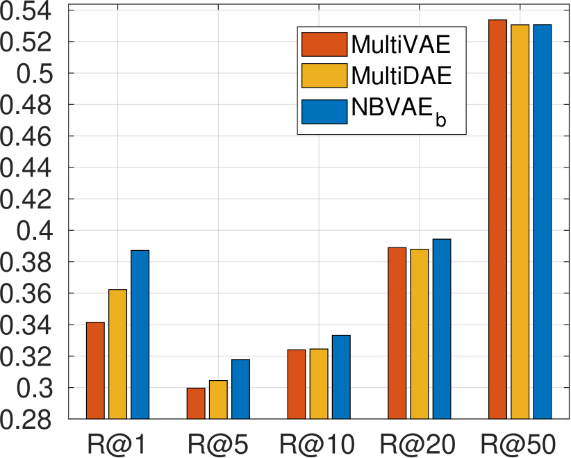
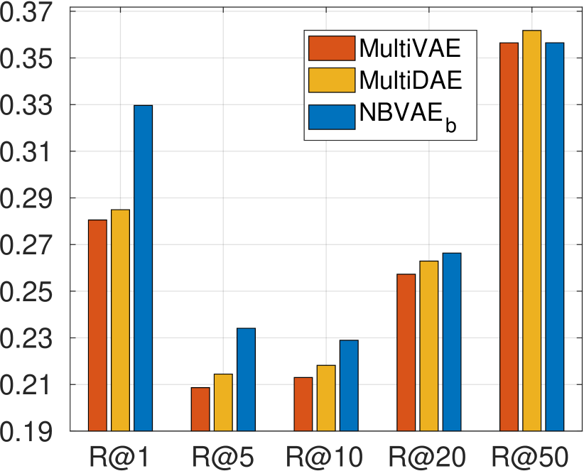
Figure 1: Comparisons of NDCG@$R$ (N@$R$) and Recall$R$ (R@$R$). Standard errors in multiple runs are generally less than 0.003 for all the models on all the datasets, which are too tiny to show in the figures.

5.2 Experiments on collaborative filtering

Our second set of experiments is targeted at collaborative filtering, where the task is to recommend items to users using their clicking history. We evaluate our models’ performance on four user-item consumption datasets: MovieLens-10M (ML-10M), MovieLens-20M (ML-20M), Netflix Prize (Netflix), and Million Song Dataset (MSD) [1]. The details of the datasets are shown in the appendix. Following Liang et al. [22], we report two evaluation metrics: Recall@$R$ and the truncated normalized discounted cumulative gain (NDCG@$R$). The calculation of the two metrics is shown in the appendix. As datasets used here are binary, we compared NBVAE${}_{\text{b}}$, with the recent VAE models: 1) MultiVAE. 2) MultiDAE [22], a denoising autoencoder (DAE) with multinomial likelihood, which introduces dropout [35] at the input layer. MultiVAE and MultiDAE are the state-of-the-art VAE models for collaborative filtering and they have been reported to outperform several recent advances such as Wu et al. [39] and He et al. [15]. The experimental settings are consistent with those in Liang et al. [22], detailed in the appendix.

Figure 1 shows the NDCG@$R$ and Recall@$R$ of the models on the four datasets, where we used $R\in\{1,5,10,20,50\}$. In general, our proposed NBVAE${}_{\text{b}}$ outperforms the baselines (i.e., MulitVAE and MultiDAE) on almost all the datasets, In particular, the margin is notably large while the $R$ value is small, such as 1 or 5. It indicates that the top-ranked items in NBVAE${}_{\text{b}}$ are always more accurate than those ranked by MultiVAE and MuliDAE. This fact is also supported by the large gap of NDCG@$R$ between NBVAE${}_{\text{b}}$ and the two baselines, as NDCG@$R$ penalises the true items that are ranked low by the model. The experimental results show that it is beneficial to treat binary data as binary rather than count-valued. We show more analysis on this point in the appendix.

5.3 Experiments on multi-label learning

Finally, we evaluate the performance of NBVAE${}_{\text{c}}$ on three multi-label learning benchmark datasets: Delicious [37], Mediamill [31], and EURLex [24]. The details of the datasets and the settings of our model are shown in the appendix. We report Precision@$R$ ($R\in\{1,3,5\}$), which is a widely-used evaluation metric for multi-label learning, following Jain et al. [19]. Several recent advances for multi-label learning are treated as the baselines, including LEML [41], PfastreXML [18], PD-Sparse [40], and GenEML [19]. For the baselines, the reported results are either obtained using publicly available implementations (with the recommended hyperparameter settings), or the publicly known best results.

Table 4: Precision (P@$R$). Best results for each dataset are in boldface. The standard errors of our model are computed in multiple runs. The results of GenEML on Delicious are not reported due to the unavailability.

Datasets	Metric	LEML	PfastreXML	PD-Sparse	GenEML	NBVAE${}_{\text{c}}$
Delicious	P@1 P@3 P@5	65.67 60.55 56.08	67.13 63.48 60.74	51.82 46.00 42.02	- - -	68.49$\pm$0.39 62.83$\pm$0.47 58.04$\pm$0.31
Mediamill	P@1 P@3 P@5	84.01 67.20 52.80	83.98 67.37 53.02	81.86 62.52 45.11	87.15 69.9 55.21	88.27$\pm$0.24 71.47$\pm$0.18 56.76$\pm$0.26
EURLex	P@1 P@3 P@5	63.40 50.35 41.28	75.45 62.70 52.51	76.43 60.37 49.72	77.75 63.98 53.24	78.28$\pm$0.49 66.09$\pm$0.17 55.47$\pm$0.15

Table 4 shows the performance comparisons on the multi-label learning datasets. It can be observed that the proposed NBVAE${}_{\text{c}}$ generally performs the best than the others on the prediction precision, showing its promising potential on multi-label learning problems. Note that the baselines are specialised to the multi-label learning problem, many of which take multiple steps of processing of the labels and features or use complex optimisation algorithms. Compared with those models, the model simplicity of NBVAE${}_{\text{c}}$ is another appealing advantage.

6 Conclusion

In this paper, we have focused on analysing and addressing two issues of PMF models on large-scale, sparse, discrete data: insufficient capability of modelling overdispersion in count-valued data and model misspecification in binary data. We have tackled those two issues by developing a VAE-based framework named NBVAE, which generates discrete data from the negative-binomial distribution. Specifically, the predictive distribution of NBVAE shows that the model can explicitly capture self-excitation because of the use of NB, and its deep structure offers better model capacity on capturing cross-excitation. By better modelling the two kinds of excitations, NBVAE is able to better handle overdispersion in count-valued data. In addition, we have developed two variants of NBVAE, NBVAE${}_{\text{b}}$ and NBVAE${}_{\text{c}}$, which are able to achieve better modelling performance on binary data and on multi-label learning. Extensive experiments have shown that NBVAE, NBVAE${}_{\text{b}}$, and NBVAE${}_{\text{c}}$ are able to achieve the state-of-the-art performance on text analysis, collaborative filtering, and multi-label learning.

See pages 1-last of appendix_pdf

References

- Bertin-Mahieux et al. [2011] Thierry Bertin-Mahieux, Daniel P.W. Ellis, Brian Whitman, and Paul Lamere. The million song dataset. In International Conference on Music Information Retrieval, 2011.
- Blei et al. [2003] David M Blei, Andrew Y Ng, and Michael I Jordan. Latent Dirichlet allocation. JMLR, 3:993–1022, 2003.
- Blei et al. [2010] David M Blei, Thomas L Griffiths, and Michael I Jordan. The nested Chinese restaurant process and Bayesian nonparametric inference of topic hierarchies. Journal of the ACM, 57(2):7, 2010.
- Bowman et al. [2016] Samuel R Bowman, Luke Vilnis, Oriol Vinyals, Andrew Dai, Rafal Jozefowicz, and Samy Bengio. Generating sentences from a continuous space. In CoNLL, pages 10–21, 2016.
- Buntine and Mishra [2014] Wray L Buntine and Swapnil Mishra. Experiments with non-parametric topic models. In SIGKDD, pages 881–890, 2014.
- Canny [2004] John Canny. Gap: a factor model for discrete data. In SIGIR, pages 122–129, 2004.
- Card et al. [2018] Dallas Card, Chenhao Tan, and Noah A Smith. Neural models for documents with metadata. In ACL, pages 2031–2040, 2018.
- Chen et al. [2014] Tianqi Chen, Emily Fox, and Carlos Guestrin. Stochastic gradient Hamiltonian Monte Carlo. In ICML, pages 1683–1691, 2014.
- Church and Gale [1995] Kenneth W Church and William A Gale. Poisson mixtures. Natural Language Engineering, 1(2):163–190, 1995.
- Cong et al. [2017] Yulai Cong, Bo Chen, Hongwei Liu, and Mingyuan Zhou. Deep latent Dirichlet allocation with topic-layer-adaptive stochastic gradient Riemannian MCMC. In ICML, pages 864–873, 2017.
- Doyle and Elkan [2009] Gabriel Doyle and Charles Elkan. Accounting for burstiness in topic models. In ICML, pages 281–288, 2009.
- Gan et al. [2015a] Zhe Gan, Changyou Chen, Ricardo Henao, David Carlson, and Lawrence Carin. Scalable deep Poisson factor analysis for topic modeling. In ICML, pages 1823–1832, 2015a.
- Gan et al. [2015b] Zhe Gan, R. Henao, D. Carlson, and Lawrence Carin. Learning deep sigmoid belief networks with data augmentation. In AISTATS, pages 268–276, 2015b.
- Grønbech et al. [2019] Christopher Heje Grønbech, Maximillian Fornitz Vording, Pascal Nordgren Timshel, Casper Kaae Sønderby, Tune Hannes Pers, and Ole Winther. scVAE: Variational auto-encoders for single-cell gene expression data. bioRxiv, page 318295, 2019.
- He et al. [2017] Xiangnan He, Lizi Liao, Hanwang Zhang, Liqiang Nie, Xia Hu, and Tat-Seng Chua. Neural collaborative filtering. In WWW, pages 173–182, 2017.
- Henao et al. [2015] Ricardo Henao, Zhe Gan, James Lu, and Lawrence Carin. Deep Poisson factor modeling. In NIPS, pages 2800–2808, 2015.
- Hoffman et al. [2013] Matthew D Hoffman, David M Blei, Chong Wang, and John Paisley. Stochastic variational inference. JMLR, 14(1):1303–1347, 2013.
- Jain et al. [2016] Himanshu Jain, Yashoteja Prabhu, and Manik Varma. Extreme multi-label loss functions for recommendation, tagging, ranking & other missing label applications. In SIGKDD, pages 935–944, 2016.
- Jain et al. [2017] Vikas Jain, Nirbhay Modhe, and Piyush Rai. Scalable generative models for multi-label learning with missing labels. In ICML, pages 1636–1644, 2017.
- Kingma and Welling [2013] Diederik P Kingma and Max Welling. Auto-encoding variational Bayes. arXiv preprint arXiv:1312.6114, 2013.
- Krishnan et al. [2018] Rahul Krishnan, Dawen Liang, and Matthew Hoffman. On the challenges of learning with inference networks on sparse, high-dimensional data. In AISTATS, pages 143–151, 2018.
- Liang et al. [2018] Dawen Liang, Rahul G Krishncan, Matthew D Hoffman, and Tony Jebara. Variational autoencoders for collaborative filtering. In WWW, pages 689–698, 2018.
- Madsen et al. [2005] Rasmus E Madsen, David Kauchak, and Charles Elkan. Modeling word burstiness using the Dirichlet distribution. In ICML, pages 545–552, 2005.
- Mencia and Fürnkranz [2008] Eneldo Loza Mencia and Johannes Fürnkranz. Efficient pairwise multilabel classification for large-scale problems in the legal domain. In ECML/PKDD, pages 50–65, 2008.
- Miao et al. [2016] Yishu Miao, Lei Yu, and Phil Blunsom. Neural variational inference for text processing. In ICML, pages 1727–1736, 2016.
- Miao et al. [2017] Yishu Miao, Edward Grefenstette, and Phil Blunsom. Discovering discrete latent topics with neural variational inference. In ICML, pages 2410–2419, 2017.
- Mnih and Salakhutdinov [2008] Andriy Mnih and Ruslan R Salakhutdinov. Probabilistic matrix factorization. In NIPS, pages 1257–1264, 2008.
- Paisley et al. [2015] John Paisley, Chong Wang, David M Blei, and Michael I Jordan. Nested hierarchical Dirichlet processes. TPAMI, 37(2):256–270, 2015.
- Ranganath et al. [2015] Rajesh Ranganath, Linpeng Tang, Laurent Charlin, and David Blei. Deep exponential families. In AISTATS, pages 762–771, 2015.
- Rezende et al. [2014] Danilo Jimenez Rezende, Shakir Mohamed, and Daan Wierstra. Stochastic backpropagation and approximate inference in deep generative models. In ICML, pages 1278–1286, 2014.
- Snoek et al. [2006] Cees GM Snoek, Marcel Worring, Jan C Van Gemert, Jan-Mark Geusebroek, and Arnold WM Smeulders. The challenge problem for automated detection of 101 semantic concepts in multimedia. In ACM MM, pages 421–430, 2006.
- Sohn et al. [2015] Kihyuk Sohn, Honglak Lee, and Xinchen Yan. Learning structured output representation using deep conditional generative models. In NIPS, pages 3483–3491. 2015.
- Srivastava and Sutton [2017] Akash Srivastava and Charles Sutton. Autoencoding variational inference for topic models. 2017.
- Srivastava et al. [2013] Nitish Srivastava, Ruslan Salakhutdinov, and Geoffrey Hinton. Modeling documents with a deep Boltzmann machine. In UAI, pages 616–624, 2013.
- Srivastava et al. [2014] Nitish Srivastava, Geoffrey Hinton, Alex Krizhevsky, Ilya Sutskever, and Ruslan Salakhutdinov. Dropout: a simple way to prevent neural networks from overfitting. JMLR, 15(1):1929–1958, 2014.
- Teh et al. [2012] Y.W. Teh, M.I. Jordan, M.J. Beal, and D.M. Blei. Hierarchical Dirichlet processes. Journal of the American Statistical Association, 101(476):1566–1581, 2012.
- Tsoumakas et al. [2008] Grigorios Tsoumakas, Ioannis Katakis, and Ioannis Vlahavas. Effective and efficient multilabel classification in domains with large number of labels. In ECML/PKDD Workshop on Mining Multidimensional Data, volume 21, pages 53–59, 2008.
- Wallach et al. [2009] Hanna M Wallach, Iain Murray, Ruslan Salakhutdinov, and David Mimno. Evaluation methods for topic models. In ICML, pages 1105–1112, 2009.
- Wu et al. [2016] Yao Wu, Christopher DuBois, Alice X Zheng, and Martin Ester. Collaborative denoising auto-encoders for top-n recommender systems. In WSDM, pages 153–162, 2016.
- Yen et al. [2016] Ian En-Hsu Yen, Xiangru Huang, Pradeep Ravikumar, Kai Zhong, and Inderjit Dhillon. PD-sparse: A primal and dual sparse approach to extreme multiclass and multilabel classification. In ICML, pages 3069–3077, 2016.
- Yu et al. [2014] Hsiang-Fu Yu, Prateek Jain, Purushottam Kar, and Inderjit Dhillon. Large-scale multi-label learning with missing labels. In ICML, pages 593–601, 2014.
- Zhou [2015] MingYuan Zhou. Infinite edge partition models for overlapping community detection and link prediction. In AISTATS, pages 1135–1143, 2015.
- Zhou [2018] Mingyuan Zhou. Nonparametric Bayesian negative binomial factor analysis. Bayesian Analysis, 2018.
- Zhou et al. [2012] Mingyuan Zhou, Lauren Hannah, David B Dunson, and Lawrence Carin. Beta-negative binomial process and Poisson factor analysis. In AISTATS, pages 1462–1471, 2012.
- Zhou et al. [2016] Mingyuan Zhou, Yulai Cong, and Bo Chen. Augmentable gamma belief networks. JMLR, 17(163):1–44, 2016.