BABAR-PUB-19/002
SLAC-PUB-17424

The BABAR Collaboration

Search for Rare or Forbidden Decays of the $D^{0}$ Meson

Abstract

We present a search for nine lepton-number-violating and three lepton-flavor-violating neutral charm decays of the type ${{D}^{0}}\rightarrow h^{\prime-}h^{-}\ell^{\prime+}{\ell^{+}}$ and ${{D}^{0}}\rightarrow h^{\prime-}h^{+}\ell^{\prime\pm}\ell^{\mp}$, where $h$ and $h^{\prime}$ represent a $K$ or $\pi$ meson and $\ell$ and $\ell^{\prime}$ an electron or muon. The analysis is based on $468$$\mbox{\,fb}^{-1}$ of ${e^{+}e^{-}}$ annihilation data collected at or close to the $\mathchar 28935\relax{(4S)}$ resonance with the BABAR detector at the SLAC National Accelerator Laboratory. No significant signal is observed for any of the twelve modes, and we establish 90% confidence level upper limits on the branching fractions in the range $(1.0-30.6)\times 10^{-7}$. The limits are between 1 and 3 orders of magnitude more stringent than previous measurements.

Lepton-flavor-violating and lepton-number-violating neutral charm decays can be used to investigate physics beyond the standard model (SM) of particle physics. A potential set of decays for study are of the form ${{D}^{0}}\rightarrow h^{\prime-}h^{-}\ell^{\prime+}{\ell^{+}}$ and ${{D}^{0}}\rightarrow h^{\prime-}h^{+}\ell^{\prime\pm}\ell^{\mp}$, where $h$ and $h^{\prime}$ represent a $K$ or $\pi$ meson and $\ell$ and $\ell^{\prime}$ an electron or muon con .

The ${{D}^{0}}\rightarrow h^{\prime-}h^{+}\ell^{\prime\pm}\ell^{\mp}$ decay modes with two opposite-charge, different-flavor leptons in the final state are lepton-flavor-violating (LFV). They are essentially prohibited in the SM because they can occur only through lepton mixing Guadagnoli and Lane (2015). The ${{D}^{0}}\rightarrow h^{\prime-}h^{-}\ell^{\prime+}{\ell^{+}}$ decay modes with two same-charge leptons are both lepton-flavor violating and lepton-number violating (LNV) and are forbidden in the SM in low-energy collisions or decays. However, LNV processes can occur in extremely high-energy or high-density interactions Klinkhamer and Manton (1984).

Lepton-number violation is a necessary condition for leptogenesis as an explanation of the baryon asymmetry of the Universe Davidson et al. (2008). If neutrinos are Majorana fermions, the neutrino and antineutrino are the same particle, and some LNV processes become possible Majorana (1937). Many models beyond the SM allow lepton-number violation. Most models have made predictions for, or used constraints from, three-body decays of the form ${D}\rightarrow Ml^{\prime}l$ or ${B}\rightarrow Ml^{\prime}l$, where $M$ is a meson Paul et al. (2011, 2014); Burdman et al. (2002); Fajfer and Prelovšek (2006); Fajfer et al. (2007); Atre et al. (2009); Yuan et al. (2013). However, some models that consider LFV and LNV four-body charm decays predict branching fractions up to ${\mathcal{O}}(10^{-6})$ to ${\mathcal{O}}(10^{-5})$, approaching those accessible with current data Atre et al. (2009); Yuan et al. (2013); Hai-Rong et al. (2015).

The branching fractions ${\mathcal{B}}({{D}^{0}}\rightarrow h^{\prime-}h^{+}{\mu^{+}\mu^{-}})$ and ${\mathcal{B}}({{D}^{0}}\rightarrow{{K}^{-}}{{\pi}^{+}}{e^{+}e^{-}})$ have recently been determined to be ${\mathcal{O}}(10^{-7})$ to ${\mathcal{O}}(10^{-6})$ Aaij et al. (2016, 2017); Lees et al. (2019), compatible with SM predictions Cappiello et al. (2013); de Boer and Hiller (2018). The most stringent existing upper limits on the branching fractions for the LFV and LNV four-body decays of the type ${{D}^{0}}\rightarrow h^{\prime-}h^{+}\ell^{\prime\pm}\ell^{\mp}$ and ${{D}^{0}}\rightarrow h^{\prime-}h^{-}\ell^{\prime+}{\ell^{+}}$ are in the range $(0.3-55.3)\times 10^{-5}$ at the 90% confidence level (C.L.) Aitala et al. (2001); Tanabashi et al. (2018); Ablikim et al. (2019). For the LFV decays ${{D}^{0}}\rightarrow V\ell^{\prime+}{\ell^{-}}$, where $V$ is an intermediate resonance such as a $\rho$ or $\phi$ meson decaying to $h^{\prime-}h^{+}$, the 90% C.L. limits are in the range $(3.4-118)\times 10^{-5}$ Freyberger et al. (1996); Aitala et al. (2001); Tanabashi et al. (2018). Searches for Majorana neutrinos in $D^{+}_{(s)}\rightarrow{{\pi}^{-}}{\mu^{+}}{\mu^{+}}$ decays have placed upper limits on the branching fractions as low as $2.2\times 10^{-8}$ at the 90% C.L. Aaij et al. (2013a).

In this report we present a search for nine ${{D}^{0}}\rightarrow h^{\prime-}h^{-}\ell^{\prime+}{\ell^{+}}$ LNV decays and three ${{D}^{0}}\rightarrow h^{\prime-}h^{+}\ell^{\prime\pm}\ell^{\mp}$ LFV decays, with data recorded with the BABAR detector at the PEP-II asymmetric-energy ${e^{+}e^{-}}$ collider operated at the SLAC National Accelerator Laboratory. The data sample corresponds to 424$\mbox{\,fb}^{-1}$ of $e^{+}e^{-}$ collisions collected at the center-of-mass (c.m.) energy of the $\mathchar 28935\relax{(4S)}$ resonance (on peak) and an additional 44$\mbox{\,fb}^{-1}$ of data collected 40 $\mathrm{\,Me\kern-1.00006ptV}$ below the $\mathchar 28935\relax{(4S)}$ resonance (off peak) Lees et al. (2013). The branching fractions for signal modes with zero, one, or two kaons in the final state are measured relative to the normalization decays ${{D}^{0}}\rightarrow{{\pi}^{-}}{{\pi}^{+}}{{\pi}^{+}}{{\pi}^{-}}$, ${{D}^{0}}\rightarrow{{K}^{-}}{{\pi}^{+}}{{\pi}^{+}}{{\pi}^{-}}$, and ${{D}^{0}}\rightarrow{{K}^{-}}{{K}^{+}}{{\pi}^{+}}{{\pi}^{-}}$, respectively. The ${D}^{0}$ mesons are identified from the decay ${{D}^{*+}}\rightarrow{{D}^{0}}{{\pi}^{+}}$ produced in ${e^{+}e^{-}}\rightarrow{{c}{\overline{c}}}$ events.

The BABAR detector is described in detail in Refs. Aubert et al. (2002, 2013). Charged particles are reconstructed as tracks with a five-layer silicon vertex detector and a 40-layer drift chamber inside a $1.5\,$T solenoidal magnet. An electromagnetic calorimeter comprised of 6580 CsI(Tl) crystals is used to identify electrons and photons. A ring-imaging Cherenkov detector is used to identify charged hadrons and to provide additional lepton identification information. Muons are identified with an instrumented magnetic-flux return.

Monte Carlo (MC) simulation is used to investigate sources of background contamination, evaluate selection efficiencies, cross-check the selection procedure, and for studies of systematic effects. The signal and normalization channels are simulated with the EvtGen package Lange (2001). We generate the signal channel decays uniformly throughout the four-body phase space, while the normalization modes include two-body and three-body intermediate resonances, as well as nonresonant decays. We also generate ${e^{+}e^{-}}\rightarrow{{q}{\overline{q}}}$ ($q=u,d,s,c$), dimuon, Bhabha elastic $e^{+}e^{-}$ scattering, ${B}{\kern 1.79993pt\overline{\kern-1.79993ptB}{}}$ background, and two-photon events Ward et al. (2003); T. Sjöstrand (1994). Final-state radiation is generated using Photos Golonka and Was (2006). The detector response is simulated with GEANT 4 Agostinelli et al. (2003); Allison et al. (2006).

In order to optimize the event reconstruction, candidate selection criteria, multivariate analysis training, and fit procedure, a rectangular area in the $m({{D}^{0}})$ versus ${\Delta m}=m({{D}^{*+}})-m({{D}^{0}})$ plane is defined, where $m({{D}^{*+}})$ and $m({{D}^{0}})$ are the reconstructed masses of the ${D}^{*+}$ and ${D}^{0}$ candidates, respectively. This optimization region is kept hidden (blinded) in data until the analysis steps are finalized. The blinded region is approximately 3 times the width of the $\Delta m$ and $m({{D}^{0}})$ resolutions. The $\Delta m$ region is $0.1447<{\Delta m}<0.1462{\mathrm{\,Ge\kern-1.00006ptV\!/}c^{2}}$ for all modes. The $m({{D}^{0}})$ signal peak distribution is asymmetric due to bremsstrahlung emission. The upper $m({{D}^{0}})$ bound on the blinded region is 1.874${\mathrm{\,Ge\kern-1.00006ptV\!/}c^{2}}$ for all modes, and the lower bound is 1.848${\mathrm{\,Ge\kern-1.00006ptV\!/}c^{2}}$, 1.852${\mathrm{\,Ge\kern-1.00006ptV\!/}c^{2}}$, and 1.856${\mathrm{\,Ge\kern-1.00006ptV\!/}c^{2}}$ for modes with two, one or no electrons, respectively.

Events are required to contain at least five charged tracks. Particle identification (PID) criteria are applied to all the charged tracks to identify kaons, pions, electrons, and muons Adam et al. (2005); Aubert et al. (2013). For modes with two kaons in the final state, the PID requirement on the kaons is relaxed compared to the single-kaon modes. This increases the reconstruction efficiency for the modes with two kaons, with little increase in backgrounds or misidentified candidates. The PID efficiency depends on the track momentum, and is in the range $0.96-0.99$ for electrons, $0.60-0.95$ for muons, and $0.90-0.98$ for kaons and pions. The misidentification probability is typically less than $0.03$ for all selection criteria, except for the pion selection criteria, where the muon misidentification rate can be as high as $0.35$ at low momentum.

Candidate ${D}^{0}$ mesons are formed from four charged tracks reconstructed with the appropriate mass hypotheses for the signal and normalization decays. The four tracks must form a good-quality vertex with a $\chi^{2}$ probability for the vertex fit greater than 0.005. A bremsstrahlung energy recovery algorithm is applied to electrons Lees et al. (2019). The invariant mass of any $e^{+}e^{-}$ pair is required to be greater than $0.1{\mathrm{\,Ge\kern-1.00006ptV\!/}c^{2}}$. For the normalization modes, the reconstructed ${D}^{0}$ meson mass is required to be in the range $1.81<m({{D}^{0}})<1.91{\mathrm{\,Ge\kern-1.00006ptV\!/}c^{2}}$, while for the signal modes, $m({{D}^{0}})$ must be in the blinded $m({{D}^{0}})$ range defined above.

The candidate ${D}^{*+}$ is formed by combining the ${D}^{0}$ candidate with a charged pion with a momentum in the laboratory frame greater than $0.1{\mathrm{\,Ge\kern-1.00006ptV\!/}c}$. For the normalization mode ${{D}^{0}}\rightarrow{{K}^{-}}{{\pi}^{+}}{{\pi}^{+}}{{\pi}^{-}}$, this pion is required to have a charge opposite to that of the final-state kaon. A vertex fit is performed with the ${D}^{0}$ mass constrained to its known value Tanabashi et al. (2018) and the requirement that the ${D}^{0}$ meson and the pion originate from the PEP-II interaction region. The $\chi^{2}$ probability of the fit is required to be greater than 0.005. For signal modes with two kaons, the mass difference $\Delta m$ is required to be $0.141<{\Delta m}<0.201{\mathrm{\,Ge\kern-1.00006ptV\!/}c^{2}}$. Signal modes with fewer than two kaons have almost no candidates beyond ${\Delta m}=0.149{\mathrm{\,Ge\kern-1.00006ptV\!/}c^{2}}$, and the range for these modes is restricted to $0.141<{\Delta m}<0.149{\mathrm{\,Ge\kern-1.00006ptV\!/}c^{2}}$.

After the application of the ${D}^{*+}$ vertex fit, the ${D}^{0}$ candidate momentum in the c.m. system, $p^{\ast}$, is required to be greater than 2.4${\mathrm{\,Ge\kern-1.00006ptV\!/}c}$. This removes most sources of combinatorial background and also charm hadrons produced in $B$ decays, which are limited to $p^{\ast}\lesssim 2.2{\mathrm{\,Ge\kern-1.00006ptV\!/}c}$ Aubert et al. (2004).

Remaining backgrounds are mainly radiative Bhabha scattering, initial-state radiation, and two-photon events, which are all rich in electrons and positrons. We suppress these backgrounds by requiring that the PID signatures of the hadron candidates be inconsistent with the electron hypothesis.

Hadronic ${D}^{0}$ decays with large branching fractions, where one or more charged tracks are misidentified as leptons, will usually have reconstructed ${D}^{0}$ masses well away from the known ${D}^{0}$ mass Tanabashi et al. (2018). To ensure rejection of this type of background. the ${D}^{0}$ candidate is also reconstructed assuming the kaon or pion mass hypothesis for the lepton candidates. If the resulting ${D}^{0}$ candidate mass is within 20${\mathrm{\,Me\kern-1.00006ptV\!/}c^{2}}$ of the known ${D}^{0}$ mass, and if $|{\Delta m}|<2{\mathrm{\,Me\kern-1.00006ptV\!/}c^{2}}$, the event is discarded. After these criteria are applied, the background from these hadronic decays is negligible.

Two particular sources of background are semileptonic charm decays in which a charged hadron is misidentified as a lepton; and charm decays in which the final state contains a neutral particle or more than four charged tracks. In both cases, tracks can be selected from elsewhere in the event to form a ${D}^{0}$ candidate. To reject these backgrounds, a multivariate selection based on a Fisher discriminant is applied Fisher (1936). The discriminant uses nine input observables: the momenta of the four tracks used to form the ${D}^{0}$ candidate; the thrust and sphericity of the ${D}^{*+}$ candidate De Rujula et al. (1978); the angle between the ${D}^{*+}$ meson candidate sphericity axis and the sphericity axis defined by the charged particles in the rest of the event (ROE); the angle between the ${D}^{*+}$ meson candidate thrust axis and the thrust axis defined by the charged particles in the ROE; and the second Fox-Wolfram moment Fox and Wolfram (1979) calculated from the entire event using both charged and neutral particles. The input observables are determined in the laboratory frame after the application of the ${D}^{*+}$ vertex fit. The discriminant is trained and tested using MC for the signal modes; for the background, data outside the optimization region, together with ${e^{+}e^{-}}\rightarrow{{c}{\overline{c}}}$ MC samples, are used. The training is performed independently for each signal mode. A requirement on the Fisher discriminant output is chosen such that approximately 90% of the simulation signal candidates are accepted. Depending on the signal mode, this rejects 30% to 50% of the background in data.

The cross feed to one signal mode from the other eleven is estimated from MC samples to be $\lesssim 0.5\%$ in all cases, assuming equal branching fractions for all signal modes. The cross feed to a specific normalization mode from the other two normalization modes is predicted from simulation to be $\lesssim 0.7\%$, where the branching fractions are taken from Ref. Tanabashi et al. (2018). Multiple candidates occur in $4.5$% to $7.1$% of simulated signal events and in $2.4$% to $4.4$% of the normalization events in data. If two or more candidates are found in an event, the one with the highest ${D}^{*+}$ vertex $\chi^{2}$ probability is selected. After the application of all selection criteria and corrections for small differences between data and MC simulation in tracking and PID performance derived from high purity control samples Aubert et al. (2013), the reconstruction efficiency $\epsilon_{\rm sig}$ for the simulated signal decays is between 3.2% and 6.2%, depending on the mode. For the normalization decays, the reconstruction efficiency $\epsilon_{\rm norm}$ is between $19.2$% and $24.7$%. The difference between $\epsilon_{\rm sig}$ and $\epsilon_{\rm norm}$ is mainly due to the momentum dependence of the lepton PID Aubert et al. (2013).

The signal mode branching fraction ${\mathcal{B}}_{\rm sig}$ is determined relative to that of the normalization decay using

$${\mathcal{B}}_{\rm sig}=\frac{N_{\rm sig}}{N_{\rm norm}}\frac{\epsilon_{\rm norm}}{\epsilon_{\rm sig}}\frac{\mathcal{L}_{\rm norm}}{\mathcal{L}_{\rm sig}}{\mathcal{B}}_{\rm norm},$$ (1)

where ${\mathcal{B}}_{\rm norm}$ is the normalization mode branching fraction Tanabashi et al. (2018), and $N_{\rm sig}$ and $N_{\rm norm}$ are the fitted yields of the signal and normalization mode decays, respectively. The symbols $\mathcal{L}_{\rm sig}$ and $\mathcal{L}_{\rm norm}$ represent the integrated luminosities of the data samples used for the signal ($468.2\pm 2.0$$\mbox{\,fb}^{-1}$) and the normalization decays ($39.3\pm 0.2$$\mbox{\,fb}^{-1}$), respectively Lees et al. (2013). For the signal modes, we use the on-peak and off-peak data samples, while the normalization modes use only a subset of the off-peak data.

Each normalization mode yield $N_{\rm norm}$ is extracted by performing an extended two-dimensional unbinned maximum likelihood (ML) fit Lees et al. (2014) to the observables $\Delta m$ and $m({{D}^{0}})$ in the range $0.141<{\Delta m}<0.149{\mathrm{\,Ge\kern-1.00006ptV\!/}c^{2}}$ and $1.81<m({{D}^{0}})<1.91{\mathrm{\,Ge\kern-1.00006ptV\!/}c^{2}}$. The measured $\Delta m$ and $m({{D}^{0}})$ values are not correlated and are treated as independent observables in the fits. The probability density functions (PDFs) in the fits depend on the normalization mode and use sums of multiple Cruijff Lees et al. (2019) and Crystal Ball Skwarnicki functions in both $\Delta m$ and $m({{D}^{0}})$. The functions for each observable use a common mean. The background is modeled with an ARGUS threshold function Albrecht et al. (1990) for $\Delta m$ and a Chebyshev polynomial for $m({{D}^{0}})$. The ARGUS end point parameter is fixed to the kinematic threshold for a ${{D}^{*+}}\rightarrow{{D}^{0}}{{\pi}^{+}}$ decay. All other PDF parameters, together with the normalization mode and background yields, are allowed to vary in the fit. The fitted yields and reconstruction efficiencies for the normalization modes are given in Table 1.

Table 1: Summary of fitted candidate yields with statistical uncertainties, systematic uncertainties, and reconstruction efficiencies for the three normalization modes.

Decay mode	$N_{\rm norm}$	Systematic	$\epsilon_{\rm norm}$
	(candidates)	(%)	(%)
${D}^{0}$ $\rightarrow$ ${{K}^{-}}{{\pi}^{+}}{{\pi}^{+}}{{\pi}^{-}}$	$260\,870\pm 520$	$4.7$	$20.1\pm 0.2$
${D}^{0}$ $\rightarrow$ ${{K}^{-}}{{K}^{+}}{{\pi}^{+}}{{\pi}^{-}}$	$8480\pm 110$	$6.6$	$19.2\pm 0.2$
${D}^{0}$ $\rightarrow$ ${{\pi}^{-}}{{\pi}^{+}}{{\pi}^{+}}{{\pi}^{-}}$	$28\,470\pm 220$	$6.8$	$24.7\pm 0.2$

Each signal mode yield $N_{\rm sig}$ is extracted by performing the ML fit with the single observable $\Delta m$ in the range $0.141<{\Delta m}<0.201{\mathrm{\,Ge\kern-1.00006ptV\!/}c^{2}}$ for signal modes with two kaons and $0.141<{\Delta m}<0.149{\mathrm{\,Ge\kern-1.00006ptV\!/}c^{2}}$ for all other signal modes. The signal PDF is a Cruijff function with parameters obtained by fitting the signal MC. The background is modeled with an ARGUS function with an end point that is set to the same value that is used for the normalization modes. The signal PDF parameters and the end point parameter are fixed in the fit. All other background parameters and the signal and background yields are allowed to vary. Figures 1 and 2 show the results of the fits to the $\Delta m$ distributions for the twelve signal modes.

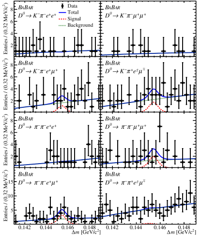
Figure 1: Projections of the unbinned maximum-likelihood fits to the final candidate distributions as a function of $\Delta m$ for the signal modes with fewer than two kaons. The solid blue line is the total fit, the dashed red line is the signal and the dotted green line is the background.

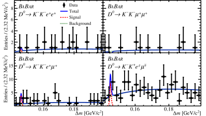
Figure 2: Projections of the unbinned maximum-likelihood fits to the final candidate distributions as a function of $\Delta m$ for the signal modes with two kaons. The solid blue line is the total fit, the dashed red line is the signal and the dotted green line is the background.

We test the performance of the ML fit for the normalization modes by generating ensembles of MC samples from the normalization and background PDF distributions. The mean numbers of normalization and background candidates used in the ensembles are taken from the fits to the data. The numbers of background and normalization mode candidates are allowed to fluctuate according to a Poisson distribution and all background and normalization mode PDF parameters are allowed to vary. No significant biases are observed in fitted yields of the normalization modes. The same procedure is repeated for the ML fit to signal modes, with ensembles of MC samples generated from the background PDF distributions only, assuming a signal yield of zero. The signal PDF parameters are fixed to the values used for the fits to the data but the signal yield is allowed to vary. The biases in the fitted signal yields are less than $\pm 0.2$ for all modes, and these are subtracted from the fitted yields before calculating the signal branching fractions.

To cross-check the normalization procedure, the signal modes in Eq. (1) are replaced with the decay ${{D}^{0}}\rightarrow{{K}^{-}}{{\pi}^{+}}$, which has a well-known branching fraction Tanabashi et al. (2018). The ${{D}^{0}}\rightarrow{{K}^{-}}{{\pi}^{+}}$ decay is selected using the same criteria as used for the ${{D}^{0}}\rightarrow{{K}^{-}}{{\pi}^{+}}{{\pi}^{+}}{{\pi}^{-}}$ mode, which is used as the normalization mode for this cross-check. The ${{D}^{0}}\rightarrow{{K}^{-}}{{\pi}^{+}}$ signal yield is $1\,881\,950\pm 1380$ with $\epsilon_{\rm sig}=(27.4\pm 0.2)\%$. We determine ${\mathcal{B}}({{D}^{0}}\rightarrow{{K}^{-}}{{\pi}^{+}})=(3.98\pm 0.08\pm 0.10)$%, where the uncertainties are statistical and systematic, respectively. This is consistent with the current world average of $(3.89\pm 0.04)$% Tanabashi et al. (2018). Similar compatibility with the ${\mathcal{B}}({{D}^{0}}\rightarrow{{K}^{-}}{{\pi}^{+}})$ world average, but with larger uncertainties, is observed when the normalization mode ${{D}^{0}}\rightarrow{{K}^{-}}{{\pi}^{+}}{{\pi}^{+}}{{\pi}^{-}}$ in Eq. (1) is replaced with the decay modes ${{D}^{0}}\rightarrow{{K}^{-}}{{K}^{+}}{{\pi}^{+}}{{\pi}^{-}}$ or ${{D}^{0}}\rightarrow{{\pi}^{-}}{{\pi}^{+}}{{\pi}^{+}}{{\pi}^{-}}$.

The main sources of systematic uncertainties in the signal yields are associated with the model parametrizations used in the fits to the signal modes and backgrounds, the fit biases, and the limited MC and data sample sizes available for the optimization of the Fisher discriminants.

The uncertainties associated with the fit model parametrizations of the signal modes are estimated by repeating the fits with alternative PDFs. This involves swapping the Cruijff and Crystal Ball functions, using Gaussian functions with different asymmetric widths, and changing the number of functions used. For the background, the order of the polynomials is changed and the ARGUS function is replaced by a second-order polynomial. The fits are also performed with the fixed signal parameters allowed to vary within the statistical uncertainties obtained from fits to the signal MC samples. The systematic uncertainty is taken as half the maximum deviation from the default fit.

The systematic uncertainties in the corrections on the fit biases for the signal yields are taken to be the statistical uncertainties on the ensembles of fits to the MC samples described above. The systematic uncertainty due to knowledge of the Fisher discriminant shape is obtained by varying the value of the selection criterion for the Fisher discriminant, changing the size of the blinded optimization region, and retraining the Fisher discriminant using a training sample with a different set of MC samples. The uncertainty is taken as half the maximum difference from the yield obtained with the default Fisher discriminant criterion. Summed together, the total systematic uncertainties in the signal yield are between 0.4 and 1.9 events, depending on the mode.

Systematic uncertainties that impact the calculation of the branching fractions of the signal modes are due to assumptions made about the distributions of the final-state particles in the signal simulation modeling, the model parametrizations used in the fits to the normalization modes, the normalization mode branching fractions, tracking and PID efficiencies, and luminosity.

Since the decay mechanism of the signal modes is unknown, we vary the angular distributions of the simulated final-state particles from the ${D}^{0}$ signal decay, where the three angular variables are defined following the prescription of Ref. Aaij et al. (2013b). We weight the reconstruction efficiencies of the phase-space simulation samples as a function of the angular-variable distributions, trying combinations of $\sin$, $\cos$, $\sin^{2}$, and $\cos^{2}$ functions. Half the maximum change in the average reconstruction efficiency is assigned as a systematic uncertainty.

Uncertainties associated with the fit model parametrizations of the normalization modes are estimated by repeating the fits with alternative PDFs for the normalization modes and backgrounds. Uncertainties in the normalization mode branching fractions are taken from Ref. Tanabashi et al. (2018). We include reconstruction efficiency uncertainties of 0.8% per track for the leptons and 0.7% for the kaon and pion Allmendinger et al. (2013). For the PID efficiencies, we assign an uncertainty of 0.7% per track for electrons, 1.0% for muons, 0.2% for pions, and 1.1% for kaons Aubert et al. (2013). A systematic uncertainty of 0.43% is associated with our knowledge of the luminosities $\mathcal{L}_{\rm norm}$ and $\mathcal{L}_{\rm sig}$ Lees et al. (2013). The total systematic uncertainties in the signal efficiencies are between 5% and 19%, depending on the mode.

We use the frequentist approach of Feldman and Cousins Feldman and Cousins (1998) to determine 90% C.L. bands that relate the true values of the branching fractions to the measured signal yields. When computing the limits, the systematic uncertainties are combined in quadrature with the statistical uncertainties in the fitted signal yields.

The signal yields for all the signal modes are compatible with zero. Table 2 gives the fitted signal yields, reconstruction efficiencies, branching fractions with statistical and systematic uncertainties, and 90% C.L. branching fraction upper limits for the signal modes.

Table 2: Summary of fitted signal yields with statistical and systematic uncertainties, reconstruction efficiencies, branching fractions with statistical and systematic uncertainties, 90% C.L. branching fraction upper limits (U.L.), and the previous limits Tanabashi et al. (2018); Ablikim et al. (2019). The branching fraction systematic uncertainties take into account correlations and cancellations between the signal and normalization modes and include the uncertainties in the normalization mode branching fractions.

					$\mathcal{B}$ 90% U.L. $(\times 10^{-7})$
Decay mode ${{D}^{0}}\rightarrow$	$N_{\rm sig}$ (candidates)		$\epsilon_{\rm sig}$ (%)	$\mathcal{B}$ $(\times 10^{-7})$	BABAR	Previous
${{\pi}^{-}}{{\pi}^{-}}{e^{+}}{e^{+}}$	$0.22\pm 3.15\pm 0.54$		$4.38\pm 0.05$	$0.27\pm 3.90\pm 0.67$	$9.1$	1120
${{\pi}^{-}}{{\pi}^{-}}{\mu^{+}}{\mu^{+}}$	$6.69\pm 4.88\pm 0.80$		$4.91\pm 0.05$	$7.40\pm 5.40\pm 0.91$	$15.2$	290
${{\pi}^{-}}{{\pi}^{-}}{e^{+}}{\mu^{+}}$	$12.42\pm 5.30\pm 1.45$		$4.38\pm 0.05$	$15.41\pm 6.59\pm 1.85$	$30.6$	790
${{\pi}^{-}}{{\pi}^{+}}{e^{\pm}}\mu^{\mp}$	$1.37\pm 6.15\pm 1.28$		$4.79\pm 0.06$	$1.55\pm 6.97\pm 1.45$	$17.1$	150
${{K}^{-}}{{\pi}^{-}}{e^{+}}{e^{+}}$	$-0.23\pm 0.97\pm 1.28$		$3.19\pm 0.05$	$-0.38\pm 1.60\pm 2.11$	$5.0$	28 Ablikim et al. (2019)
${{K}^{-}}{{\pi}^{-}}{\mu^{+}}{\mu^{+}}$	$-0.03\pm 2.10\pm 0.40$		$3.30\pm 0.05$	$-0.05\pm 3.34\pm 0.64$	$5.3$	3900
${{K}^{-}}{{\pi}^{-}}{e^{+}}{\mu^{+}}$	$3.87\pm 3.96\pm 2.36$		$3.48\pm 0.04$	$5.84\pm 5.97\pm 3.56$	$21.0$	2180
${{K}^{-}}{{\pi}^{+}}{e^{\pm}}\mu^{\mp}$	$2.52\pm 4.60\pm 1.35$		$3.65\pm 0.05$	$3.62\pm 6.61\pm 1.95$	$19.0$	5530
${{K}^{-}}{{K}^{-}}{e^{+}}{e^{+}}$	$0.30\pm 1.08\pm 0.41$		$3.25\pm 0.04$	$0.43\pm 1.54\pm 0.58$	$3.4$	1520
${{K}^{-}}{{K}^{-}}{\mu^{+}}{\mu^{+}}$	$-1.09\pm 1.29\pm 0.42$		$6.21\pm 0.06$	$-0.81\pm 0.96\pm 0.32$	$1.0$	940
${{K}^{-}}{{K}^{-}}{e^{+}}{\mu^{+}}$	$1.93\pm 1.92\pm 0.83$		$4.63\pm 0.05$	$1.93\pm 1.93\pm 0.84$	$5.8$	570
${{K}^{-}}{{K}^{+}}{e^{\pm}}\mu^{\mp}$	$4.09\pm 3.00\pm 1.59$		$4.83\pm 0.05$	$3.93\pm 2.89\pm 1.45$	$10.0$	1800

In summary, we report 90% C.L. upper limits on the branching fractions for nine lepton-number-violating ${{D}^{0}}\rightarrow h^{\prime-}h^{-}\ell^{\prime+}{\ell^{+}}$ decays and three lepton-flavor-violating ${{D}^{0}}\rightarrow h^{\prime-}h^{+}\ell^{\prime\pm}\ell^{\mp}$ decays. The analysis is based on a sample of ${e^{+}e^{-}}$ annihilation data collected with the BABAR detector, corresponding to an integrated luminosity of $468.2\pm 2.0$$\mbox{\,fb}^{-1}$. The limits are in the range $(1.0-30.6)\times 10^{-7}$ and are between 1 and 3 orders of magnitude more stringent than previous results.

We are grateful for the excellent luminosity and machine conditions provided by our PEP-II colleagues, and for the substantial dedicated effort from the computing organizations that support BABAR. The collaborating institutions wish to thank SLAC for its support and kind hospitality. This work is supported by DOE and NSF (USA), NSERC (Canada), CEA and CNRS-IN2P3 (France), BMBF and DFG (Germany), INFN (Italy), FOM (The Netherlands), NFR (Norway), MES (Russia), MINECO (Spain), STFC (United Kingdom), BSF (USA-Israel). Individuals have received support from the Marie Curie EIF (European Union) and the A. P. Sloan Foundation (USA).

References

- (1) Charge conjugation is implied throughout.
- Guadagnoli and Lane (2015) D. Guadagnoli and K. Lane, Phys. Lett. B 751, 54 (2015).
- Klinkhamer and Manton (1984) F. R. Klinkhamer and N. S. Manton, Phys. Rev. D 30, 2212 (1984).
- Davidson et al. (2008) S. Davidson, E. Nardi, and Y. Nir, Phys. Rep. 466, 105 (2008).
- Majorana (1937) E. Majorana, Nuovo Cim. 14, 171 (1937).
- Paul et al. (2011) A. Paul, I. I. Bigi, and S. Recksiegel, Phys. Rev. D 83, 114006 (2011).
- Paul et al. (2014) A. Paul, A. de la Puente, and I. I. Bigi, Phys.Rev. D 90, 014035 (2014).
- Burdman et al. (2002) G. Burdman, E. Golowich, J. A. Hewett, and S. Pakvasa, Phys. Rev. D 66, 014009 (2002).
- Fajfer and Prelovšek (2006) S. Fajfer and S. Prelovšek, Phys. Rev. D 73, 054026 (2006).
- Fajfer et al. (2007) S. Fajfer, N. Košnik, and S. Prelovšek, Phys. Rev. D 76, 074010 (2007).
- Atre et al. (2009) A. Atre, T. Han, S. Pascoli, and B. Zhang, J. High Energy Phys. 05, 030 (2009).
- Yuan et al. (2013) H. Yuan, T. Wang, G.-L. Wang, W.-L. Ju, and J.-M. Zhang, J. High Energy Phys. 08, 066 (2013).
- Hai-Rong et al. (2015) D. Hai-Rong, F. Feng, and L. Hai-Bo, Chin. Phys. C 39, 013101 (2015).
- Aaij et al. (2016) R. Aaij et al. (LHCb Collaboration), Phys. Lett. B 757, 558 (2016).
- Aaij et al. (2017) R. Aaij et al. (LHCb Collaboration), Phys. Rev. Lett. 119, 181805 (2017).
- Lees et al. (2019) J. P. Lees et al. (BABAR Collaboration), Phys. Rev. Lett. 122, 081802 (2019).
- Cappiello et al. (2013) L. Cappiello, O. Cata, and G. D’Ambrosio, J. High Energy Phys. 04, 135 (2013).
- de Boer and Hiller (2018) S. de Boer and G. Hiller, Phys. Rev. D 98, 035041 (2018).
- Aitala et al. (2001) E. M. Aitala et al. (E791 Collaboration), Phys. Rev. Lett. 86, 3969 (2001).
- Tanabashi et al. (2018) M. Tanabashi et al. (Particle Data Group), Phys. Rev. D 98, 030001 (2018).
- Ablikim et al. (2019) M. Ablikim et al. (BESIII Collaboration), Phys. Rev. D 99, 112002 (2019).
- Freyberger et al. (1996) A. Freyberger et al. (CLEO Collaboration), Phys. Rev. Lett. 76, 3065 (1996).
- Aaij et al. (2013a) R. Aaij et al. (LHCb Collaboration), Phys. Lett. B 724, 203 (2013a).
- Lees et al. (2013) J. P. Lees et al. (BABAR Collaboration), Nucl. Instrum. Methods Phys. Res., Sect. A 726, 203 (2013).
- Aubert et al. (2002) B. Aubert et al. (BABAR Collaboration), Nucl. Instrum. Methods Phys. Res., Sect. A 479, 1 (2002).
- Aubert et al. (2013) B. Aubert et al. (BABAR Collaboration), Nucl. Instrum. Methods Phys. Res., Sect. A 729, 615 (2013).
- Lange (2001) D. J. Lange, Nucl. Instrum. Methods Phys. Res., Sect. A 462, 152 (2001).
- Ward et al. (2003) B. F. L. Ward, S. Jadach, and Z. Was, Nucl. Phys. Proc. Suppl. 116, 73 (2003).
- T. Sjöstrand (1994) T. Sjöstrand, Comput. Phys. Commun. 82, 74 (1994).
- Golonka and Was (2006) P. Golonka and Z. Was, Eur. Phys. J. C 45, 97 (2006).
- Agostinelli et al. (2003) S. Agostinelli et al. (GEANT 4 Collaboration), Nucl. Instrum. Methods Phys. Res., Sect. A 506, 250 (2003).
- Allison et al. (2006) J. Allison, K. Amako, J. Apostolakis, H. Araujo, P. Dubois, et al. (GEANT 4 Collaboration), IEEE Trans. Nucl. Sci. 53, 270 (2006).
- Adam et al. (2005) I. Adam et al., Nucl. Instrum. Methods Phys. Res., Sect. A 538, 281 (2005).
- Aubert et al. (2004) B. Aubert et al. (BABAR Collaboration), Phys. Rev. D 69, 111104 (2004).
- Fisher (1936) R. A. Fisher, Ann. Eugen. 7, 179 (1936).
- De Rujula et al. (1978) A. De Rujula, J. R. Ellis, E. G. Floratos, and M. K. Gaillard, Nucl. Phys. B138, 387 (1978).
- Fox and Wolfram (1979) G. C. Fox and S. Wolfram, Nucl. Phys. B149, 413 (1979).
- Lees et al. (2014) J. P. Lees et al. (BABAR Collaboration), Phys. Rev. D 89, 011102 (2014).
- (39) T. Skwarnicki, A study of the radiative cascade transitions between the and resonances, Ph.D. thesis, Institute of Nuclear Physics, Krakow, DESY-F31-86-02, 1986.
- Albrecht et al. (1990) H. Albrecht et al. (ARGUS Collaboration), Phys. Lett. B 241, 278 (1990).
- Aaij et al. (2013b) R. Aaij et al. (LHCb Collaboration), Phys. Rev. D 88, 052002 (2013b).
- Allmendinger et al. (2013) T. Allmendinger et al., Nucl. Instrum. Methods Phys. Res., Sect. A 704, 44 (2013).
- Feldman and Cousins (1998) G. J. Feldman and R. D. Cousins, Phys. Rev. D 57, 3873 (1998).