Social Network of Extreme Tweeters: A Case Study

Abstract

The number of posts made by a single user account on a social media platform Twitter in any given time interval is usually quite low. However, there is a subset of users whose volume of posts is much higher than the median. In this paper, we investigate the content diversity and the social neighborhood of these extreme users and others. We define a metric called “interest narrowness”, and identify that a subset of extreme users, termed anomalous users, write posts with very low topic diversity, including posts with no text content. Using a few interaction patterns we show that anomalous groups have the strongest within-group interactions, compared to their interaction with others. Further, they exhibit different information sharing behaviors with other anomalous users compared to non-anomalous extreme tweeters.

I Introduction

Social Media is part of our daily lives, and increasingly more people are actively participating in various social media platforms. It was recently reported [10] that Twitter has 126 million daily users, with an estimated annual growth rate of about 9%. It is estimated that roughly 46% of Twitter users are on the platform daily. In this paper, we investigate the following questions: What types of users tweet an enormous amount and what do they talk about?

The intuition behind this paper comes from the observation that we can characterize users’ tweeting behavior based on the volume and the content diversity of their tweets.

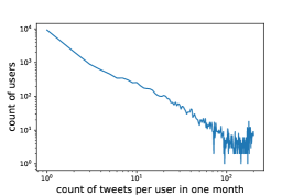
We first consider tweet volumes for individual users. How often do people tweet? Based on our data set of over 1.5 billion tweets, we observe that over any arbitrary time interval, the number of tweets by a user follows a power law type of distribution (see Fig. 1 for a typical distribution for one month) – most users post very few tweets while only a few users write considerably more tweets. In the empirical result shown in Fig. 1, only 20% of the users posted more than 24 tweets in July 2017. We use the term extreme tweeters (ETT) for users who tweet more frequently than an average user in any given time interval (we give a more precise definition later).

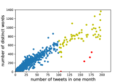
A different stratification of users can be created based on the content diversity (c-diversity) of their posts. Intuitively, a user who is interested in many topics will have a higher content diversity than a user with a narrow range of interests (e.g., only football). One simple, but rough measure of c-diversity is the number of distinct words (not counting mentions) used by a user over all their posts in a given period of time. Fig. 1 shows a typical plot of the c-diversity of users as a function of the number of tweets they sent. In general, users who tweet more tend to have higher c-diversity. Clustering the frequency distribution reveals three different clusters corresponding to (a) users who tweet less and and use fewer distinct words (blue cluster), (b) users who tweet more and have higher content diversity (greenish yellow cluster), and (c) the small number of users who tweet more and yet have low content diversity (red cluster).

In this case study, we explore the tweeting behavior as well as the social network of ETT, who constitute groups (b) and (c) above. We are particularly interested in group (c) because at first glance, their high-tweet-rate, low-diversity behavior is anomalous and appears somewhat counterintuitive. In the light of this exploration, the paper makes the following contributions:

1. We propose a novel way to classify users based on their tweet rate and a new measure of verbosity called interest narrowness.

2. We present an algorithm to detect the anomalous users.

3. We investigate the nature of the network relations of the anomalous group and the other groups.

4. We show that the social interaction of anomalous and non-anomalous groups vary with time, and the vigorousness of the interaction intensifies around events like elections.

Figure 1: (a) Frequency distribution of tweet count for users in a month. (b) Frequency distribution of distinct words vs. number of tweets in a month.

I-A Related Work

The problem of user characterization in a social network has been investigated by many research groups. We present a few samples of these research efforts.

A 2016 survey [11] covers a wide bandwidth of different approaches for user characterization. The behavioral properties they report range from conscientiousness and extroversion to privacy behavior, deceptive traits and response to social attacks. In contrast to our approach, many of the reported analyses studied in this paper are based on focused user surveys.

Gabrowicz et al [5] take a bond-theory based approach and distinguish between social user groups and topical user groups in a network based on features like reciprocity, topicality and activity. Of these, topicality, defined based on a metric called “normalized entropy” measures how much the topics of discussion vary within a group. The higher the entropy, the greater is the variety of terms and, according to the theory, the more social the group is. However, this measure considers the words to be independent, which usually does not hold.

Similar to our notion of anomalous users, [8] investigates the concept of “dedicators”, users who transmit information in selected topic areas to the people in their egocentric networks. The concept of dedication is determined by volume, engagement, personal tendencies and topic weight, where personal tendency includes the user’s topic diversity as measured by Latent Dirichlet Allocation (LDA), and engagement measures the activity level of conversations.

Diversity of topics within text posts is also analyzed in papers like [9] that perform LDA to compute topics and then determine topic diversity across a user’s posts as the number of distinct probable topics found across all of the user’s posts.

Closer to our application, Bail et al [2] used a POS-tagged BOW model to analyze Facebook posts for political content and derived a network of correlated concepts. They demonstrated how some advocacy organizations produce social media messages that inspire far-ranging conversation among social media users. Interestingly, their network analysis is based on the co-occurrence of concept terms from which they extract interesting connection patterns that characterize influence modalities for advocacy groups.

In contrast to all related work, ours is the first attempt, to our knowledge, that specifically analyzes the posting behavior and interaction patterns of extreme tweeters. Although we use Twitter as our example social media platform, our method is equally valid for any other platform that exhibits high-volume postings and vigorous interactions.

II The Setting

II-A User Behavior Classification

We now formalize the intuitive user behavior classification scheme presented in Section I.

II-A1 Classification based on Tweet Volume

Assume that $W$ is the time window of observation (e.g., 24 months), and $\Delta\ll W$ is the minimal analytic interval (MAI), i.e., a minimum time-interval (e.g., 1 week) over which data is collected in order to perform any user behavior analysis. We denote consecutive MAIs as $\Delta_{1},\Delta_{2}\ldots\Delta_{n}$ within $W$.

Definition 1 (ETT Behavior)

Let $U$ be the set of users, and $T^{u}(\Delta_{i})$ be the number of posts by a user $u\in U$ in $i$-th MAI $\Delta_{i}$, then we say an user $u^{\prime}$ exhibits ETT behavior in $\Delta_{i}$ if $T^{u^{\prime}}(\Delta_{i})\geq\mathbf{E}\left[T^{u}_{\Delta_{i}}\right]+\delta\cdot\sqrt{\mathbf{Var}\left[T^{u}_{\Delta_{i}}\right]}$, where $\delta\geq 0$ is an arbitrary constant to control the selectivity.

Definition 2 (ETT Interval)

If a user $u$ exhibits ETT behavior in MAI {$\Delta^{u}_{i},\Delta^{u}_{j}\ldots\Delta^{u}_{l}$}, then the ETT interval of user $u$ is defined as the concatenation of consecutive subintervals from {$\Delta^{u}_{k}$}.

Often a single user would not have a single continuous period of hyperactivity, but several ETT intervals within an observation window. We can use both the longest ETT interval (LETTI), and the total ETT interval (TETTI) as measures of a user’s sustained ETT behavior. In this paper, we simply classify users with no associated ETT intervals as regular users, and users with at least one ETT interval as ETT users.

II-A2 Classification based on Content Diversity

In Section I, we used the number of distinct words as a rough measure of c-diversity for a user. However, it is not a suitable measure of c-diversity because it actually measures the vocabulary diversity of a user. While a low-vocabulary user will have lower c-diversity than a high-vocabulary user, the measure cannot well distinguish between the c-diversities of two users with comparable vocabulary sizes. Secondly, just the raw count of words does not capture the thematic diversity of a user. Although two users have comparable vocabulary sizes, one may cover more themes than the other. In Section III, we develop a new measure called Interest Narrowness by taking a topic model type approach.

III Measuring Interest Narrowness

We use the bag-of-words and singular value decomposition (SVD) techniques to develop the Interest Narrowness measure. For a user $u$, we construct its text matrix $\mathbf{M}^{u}$ by adopting the bag-of-words model on all tweets of $u$ during a certain period of time. Let $p$ be the tweet count of $u$ and $q$ be the number of distinct words (except stop words and URLs) over all tweets of $u$. Apparently, $\mathbf{M}^{u}$ is of dimension $p\times q$, and without loss of generality, we assume that $p\leq q$. Apply SVD to $\mathbf{M}^{u}$:

$$\mathbf{M}^{u}=\mathbf{U}\mathbf{\Sigma}^{u}\mathbf{V},$$ (1)

where $\mathbf{U}$ and $\mathbf{V}$ are $p\times p$ and $q\times q$ unitary matrices respectively and $\mathbf{\Sigma}^{u}$ is a matrix where the diagonal entries $\sigma_{i}^{u}=\mathbf{\Sigma}^{u}_{i,i}$ are singular values. Equivalently, $\mathbf{M}^{u}$ can be rewritten by a weighted sum of $p$ separable matrices:

$$\mathbf{M}^{u}=\sum_{i}\mathbf{A}_{i}^{u}=\sum_{i}\sigma_{i}^{u}\cdot\mathbf{U}_{i}\otimes\mathbf{V}_{i},$$ (2)

where $\mathbf{U}_{i}$ and $\mathbf{V}_{i}$ are the $i^{th}$ columns of $\mathbf{U}$ and $\mathbf{V}$ respectively, and $\otimes$ refers to the outer product. Based on Eq. (2), we define the contribution of $j^{th}$ separable matrix $\mathbf{A}^{u}_{j}$ as follows,

$$c^{u}_{j}=\frac{{\sigma_{j}^{u}}^{2}}{\sum_{i}\sigma_{i}^{u2}}.$$ (3)

III-1 Exact SVD Based Measure (EM)

Assume that separable matrices $\mathbf{A}^{u}_{1},\cdots,\mathbf{A}^{u}_{p}$ are sorted in descending order by their corresponding singular values. Given a threshold $d\in[0,1]$, let $K$ denote the minimum value of $k$ such that

$$\sum_{j=1}^{k}c_{j}^{u}=\frac{\sum_{j=1}^{k}\sigma_{j}^{u2}}{\sum_{i}\sigma_{i}^{u2}}\geq d.$$

Thus $K$ is the minimum number of $k$ such that the top-$k$ separable matrices can explain $d\times 100\%$ of matrix $\mathbf{M}^{u}$. In other words, the first $K$ columns of $\mathbf{V}$ can represent most of the topics of $u$’s tweets. Naturally, the interest narrowness of user $u$ can be defined as,

$$\gamma^{u}=1-\frac{K}{p}.$$ (4)

Notably, the bottleneck of the exact measurement is the computation of SVD on text matrix $\mathbf{M}^{u}$, which takes time $O(\min(p^{2}q,pq^{2}))$.

III-2 Randomized SVD based Measure (RM)

Evaluation for the first measure for all ETT users is expensive since both the size of the text matrix and the number of ETT users can be large. To speed up the computation, we can approximate matrix decomposition by using the randomized SVD [6] where only partial singular values are computed. For a user $u$ with text matrix $\mathbf{M}^{u}$ of dimension $p\times q$, it can be approximated by

$$\mathbf{M}^{u}\approx\widetilde{\mathbf{U}}\widetilde{\mathbf{\Sigma}}^{u}\widetilde{\mathbf{V}},$$ (5)

where $\widetilde{\mathbf{U}}$ is of $p\times k$, $\widetilde{\mathbf{V}}$ is of $k\times q$ and $\widetilde{\mathbf{\Sigma}}^{u}$ is of $k\times k$ where $k<\min(p,q)$. The interest narrowness is then given by,

$$\eta^{u}=\frac{\sum_{j=1}^{k}\widetilde{\sigma_{j}}^{u2}}{\sum_{i}\sigma_{i}^{u2}}=\frac{\sum_{j=1}^{k}\widetilde{\sigma_{j}}^{u2}}{||\mathbf{M}^{u}||_{F}^{2}},$$ (6)

where ${||\mathbf{M}^{u}||_{F}}$ is the Frobenius norm of matrix $\mathbf{M}^{u}$ and $||\mathbf{M}^{u}||_{F}^{2}=\sum_{i=1}^{p}\sum_{j=1}^{q}|m_{ij}^{u}|^{2}=\sum_{i=1}\sigma_{i}^{u2}$. The commonly used implementation of randomized SVD takes time $O(pq\log k+(p+q)k^{2})$ [3]. Notice that $k$ serves as a hyper-parameter in the computation of narrowness. In our experiments we have noticed that setting $k$ to $\max(10,p/10)$ can well represent the c-diversity of all tweets. For this fixed setting of $k$, a large $\eta$ stands for relatively narrow topic interests.

Given any time interval $I=[t_{s},t_{e}]$, we can define anomalous users (shown as red cluster in Fig. 1) as a user with ETT behavior and narrow topic interests during $I$. Algorithm 1 provides the framework to detect anomalous users based on the definition.

Input: a list of triples: $\mathcal{T}=\{(T.u,T.text,T.time)\}$, a fixed time period: $I$, and hyper-parameters: $\delta$ and $\lambda$

Output: a list of anomalous users: $\mathcal{A}$

/* Step 1: Find ETTs */

1 $T^{\prime}\leftarrow\{(T.u,T.text)|T\in\mathcal{T},T.time\in I\}$;

2 group by users to get per user tweet count and tweet corpus as $\mathcal{C}\leftarrow\{(C.u,C.count,C.all\_texts)\}$;

3 $ETT\leftarrow\{C.u|C\in\mathcal{C},C.count\geq\mathbf{E}\left[\mathcal{C}.count\right]+\delta\sqrt{\mathbf{Var}\left[\mathcal{C}.count)\right]}$;

/* Step 2: Calculate Narrowness */

4 $N\leftarrow max(\{C.count|C\in\mathcal{C}\})$;

5 get the maximum number of distict words for individual user $D\leftarrow max(\{C.distinct\_word|C\in\mathcal{C}\})$;

6 $\mathcal{H}\leftarrow\{\}$;

7 if $N\times D\leq M$ then

8      for $u\in ETT$ do

9            use EM (Eq. (4)) to calculate interest narrowness $nrw$ for $u$;

10             $\mathcal{H}$.add($(u,nrw)$);

11      

12else

13       for $u\in ETT$ do

14            use RM (Eq. (6)) to calculate interest narrowness $nrw$ for $u$;

15             $\mathcal{H}$.add($(u,nrw)$);

16      

/* Step 3: Find Anomalous Users */

17 $\mathcal{A}\leftarrow\{H.u|H\in\mathcal{H},H.nrw\geq\mathbf{E}\left[\mathcal{H}.nrw\right]+\lambda\sqrt{\mathbf{Var}\left[\mathcal{H}.nrw)\right]}$;

18

Algorithm 1 Anomalous User Detection

Algorithm 1 takes a list of $(user,text,time)$ triples as input and outputs all users with ETT behavior and high interest narrowness. The algorithm has two hyper-parameters, $\delta$ and $\lambda$, which jointly control the selectivity of anomalous users. Intuitively, the larger $\delta$ and $\lambda$ are, the more strict the criteria of anomalous users will be. The algorithm consists of two steps. Given a time period $I$, lines 1-3 constitute step 1 where all users who exhibit ETT behavior in $I$ are found based on Definition 1. For each of these users, lines 4-14 calculate its interest narrowness. Notably, we set a threshold $M$ to decide whether or not to apply the randomized SVD based measure (RM). If the possible largest size of text matrix, i.e., $N\cdot D$, is smaller than $M$, the exact SVD based measure (EM) is adopted; otherwise, RM is performed for efficiency consideration. In our setting, $M$ is set to be $2,000\times 5,000$, which is experimentally demonstrated to reach a balance between efficiency and effectiveness. Finally, line 15 finds out users from ETT with high interest narrowness values as anomalous users.

The complexity of Algorithm 1 comes primarily from the computation of SVD for each user in $ETT$. If the exact version of SVD is adopted, the total time complexity is $O(|ETT|\cdot\min(ND^{2},DN^{2}))$, where $N$ and $D$ represent the maximum tweet count and the maximum number of distinct words, respectively. Otherwise, the total complexity should be $O(|ETT|\cdot[ND\log k+(N+D)k^{2}])$.

We choose the randomized SVD based algorithm rather than the more standard LDA technique [8, 9] based on the following considerations. First, the number of potential topics is hard to set, especially in our setting where the topics are computed per user and we have potentially many users. Second, when the tweet count of one user is not big enough, SVD gives more meaningful results than LDA because the quality of LDA-produced topics is satisfactory when the training set is large. Finally, the interest narrowness not only depends on the number of topics, but on within-topic term-diversity as well.

IV Social Network Analysis

IV-A Rationale

So far, we have focused on the ETT behavior of users and identified narrow-interest users with ETT behavior. We now explore the social network around these users to study their interaction patterns with other users, as well as the conversation topics of their network neighborhoods. We would like to investigate four questions about anomalous users:

1. Do anomalous users interact heavily with each other?

2. Do anomalous users interact heavily with extreme tweeters or regular users?

3. If some anomalous users interact heavily with each other, what is their behavior pattern as a group?

4. Do anomalous users have different behaviors during different time periods, especially around major public-opinion-inciting events?

The anomalous users themselves constitute a very small part of the larger social network that is induced by various forms of communication (reply, retweets, mentions, etc.) between any pair of users. We seek to identify connection patterns in network neighborhoods of the users of interest. In the following section, we present a few simple connection patterns amongst the anomalous users, the non-anomalous users with ETT behavior and regular users, and Section V shows that these patterns suffice to bring out some distinctive characteristics of anomalous users.

IV-B Three Simple Patterns

In Fig. 2 we show three simple connection patterns involving the three user categories. There are three types of nodes in the pattern graph: red nodes represent anomalous users, blue nodes represent extreme tweeters and white nodes represent regular users. Edges of the graph are undirected because in this case study we are simply exploring the connections and not the direction of messages that flow between user groups.

The first connection pattern (called Type-I hereafter), denoted as $G_{1}=(V_{1},E_{1})$, shows only within-group triads for anomalous users. The edges represent the mentions relationship between two anomalous users: $(v_{i},v_{j})\in E_{1}$ if $v_{i}$ mentions $v_{j}$ or $v_{j}$ mentions $v_{i}$ during a certain time period $T$. The second connection pattern (Type-II), denoted as $G_{2}=(V_{2},E_{2})$, extends the triads to include first neighbors of anomalous users who are also extreme tweeters in the same time period. $V_{2}$ is the set of anomalous users and extreme tweeters who are mentioned by or mention an anomalous user, and edges $E_{2}$ also include the mentions between these non-anomalous ETT users. As for the third case, the pattern network (Type-III) is formed by considering anomalous users and all their first neighbors. These three patterns correspond to the questions Q1 and Q2 posed in Section IV-A.

Figure 2: Three connection patterns around anomalous users.

IV-C Metrics

In this subsection, we propose three measures to assess the connectivity and density of our connection patterns in the network during any time interval. With these measures we expect to evaluate the interaction intensity of anomalous users and their neighbors (Q1 and Q2), and capture the group behavior pattern (Q3) of the anomalous user group and their immediate neighborhood.

IV-C1 Coreness Distribution

$k$-core is a standard technique for tasks like dense region detection [4, 1] and network feature extraction for different kinds of social network analysis [12, 7]. We recall that the coreness of a vertex in a graph is $k$ if it belongs to a $k$-core, but not to a $(k+1)$-core. In this paper, we use the terms “coreness” and “core number” interchangeably.

Let $G^{T}$ be the complete social network within time interval $T$. To capture the holistic connective characteristic of anomalous users and their related users in $G^{T}$, we introduce the concept of “coreness distribution”, which is the distribution of coreness of nodes in the largest subgraph of $G^{T}$ satisfying a certain connection pattern (i.e., Type-I, Type-II or Type-III). Specifically, to measure the connection intensity among anomalous users, we extract the largest subgraph of $G^{T}$ satisfying the Type-I pattern, denoted by $G^{T}_{1}$, which would include all anomalous users, and then calculate core number of all users in $G^{T}_{1}$ to get the coreness distribution. As $G^{T}_{1}$ only includes the relations among anomalous users, the coreness distribution of $G^{T}_{1}$ would give an answer to Q1 from Section IV-A. If the distribution shows that a subset of users have relatively high coreness, we can conclude that these anomalous users interact intensively with each other. Similarly, to capture how intensely do anomalous users interact with extreme tweeters (or regular users), the largest subgraph of $G^{T}$ satisfying Type-II pattern (resp. Type-III pattern), say $G^{T}_{2}$ (or $G^{T}_{3}$), is constructed, and the coreness distribution of anomalous users in $G^{T}_{2}$ (or $G^{T}_{3}$) is calculated and compared with that of $G^{T}_{1}$.

IV-C2 Measure of Collective Behavior

The coreness distribution depicts the holistic interaction intensity of all anomalous users with different categories of users, which answers Q1 and Q2. However, it is possible that an anomalous user may not strongly connect with other anomalous users. We focus on the group of strongly connected anomalous users (Q3), defined as follows.

Definition 3 (Anomalous Group)

Let $G_{A}^{T}$ be a subgraph of $G^{T}$ satisfying,

• Pattern Constraint: $G_{A}^{T}$ satisfies Type-I pattern;

• Strongest Connection: $G_{A}^{T}$ is a $k$-core where $k$ is the largest degeneracy value among all subragphs of $G^{T}$ satisfying Type-I pattern;

• Maximality: There does not exist another $k$-core satisfying Type-I pattern that is a supergraph of $G_{A}^{T}$.

Then the nodes of $G_{A}^{T}$, say $\mathcal{A}$, form one anomalous group with coreness $k^{\mathcal{A}}_{1}=k$.

Lemma 1

For any graph $G$ satisfying Type-$x$ connection pattern, $x=1,2,3$, any subgraph of $G$ also satisfies Type-$x$ pattern.

Based on Lemma 1, an anomalous group is, by definition, the maximal $k$-core of $G^{T}_{1}$ where $k$ is the maximum coreness value of nodes in $G^{T}_{1}$. In Type-II or Type-III connection patterns, users in an anomalous group may act collaboratively (i.e., they mention similar users), or they may have diverse behaviors (i.e., they interact with different users). To measure such interaction patterns, we define the coreness of anomalous group and then present two metrics.

Definition 4 (Coreness of Anomalous Group)

For an anomalous group $\mathcal{A}$, let $G^{T}_{A_{x}}$ be a subgraph of $G^{T}$ such that,

• $G^{T}_{A_{x}}$ satisfies Type-$x$ pattern where $x$ can be 1, 2, or 3.

• The nodes of $G^{T}_{A_{x}}$ is a superset of $\mathcal{A}$.

• $G^{T}_{A_{x}}$ is a $k^{\mathcal{A}}_{x}$-core where $k^{\mathcal{A}}_{x}$ is the largest degeneracy value among all subgraphs of $G^{T}$ satisfying Type-$x$ pattern and including nodes $\mathcal{A}$.

We say $k^{\mathcal{A}}_{x}$ is the coreness of $\mathcal{A}$ in Type-$x$ pattern.

Obviously, $k^{\mathcal{A}}_{2}$ and $k^{\mathcal{A}}_{3}$ would be at least $k^{\mathcal{A}}_{1}$ because Type-II or III is an extension of Type-I pattern. From Lemma 1, $k^{\mathcal{A}}_{2}$ and $k^{\mathcal{A}}_{3}$ can be calculated as $\min\{C=\{c_{u}|u\in\mathcal{A}\}\}$, where $c_{u}$ is the coreness of $u$ in $G^{T}_{2}$ or $G^{T}_{3}$, which are the largest subgraphs of $G^{T}$ satisfying Type-II or Type-III patterns respectively.

We extract the maximal $k^{\mathcal{A}}_{2}$-core and $k^{\mathcal{A}}_{3}$-core including $\mathcal{A}$ from $G^{T}_{2}$ and $G^{T}_{3}$ respectively. These cores could be considered as a group of users who highly interact with $\mathcal{A}$. To evaluate the behaviors of group $\mathcal{A}$, we provide the following measures.

Definition 5 (Common Neighbor Ratio and Diversity Ratio)

Let $\mathcal{A}$ be an anomalous group, and $\mathcal{U}$ denote the set of other nodes in the $k^{\mathcal{A}}_{2}$-core or $k^{\mathcal{A}}_{3}$-core of subgraph $G^{T}_{2}$ or $G^{T}_{3}$. Define the common neighbor ratio (CNR) as,

$$r=\frac{\sum_{u\in\mathcal{U}}{N_{u}}}{|\mathcal{A}||\mathcal{U}|},$$ (7)

where $N_{u}$ is the number of anomalous users in $\mathcal{A}$ who are connected to a user $u$. The diversity ratio (DR) is defined as,

$$\beta=\frac{|\{u|u\in\mathcal{U},N_{u}\geq r\times|\mathcal{A}|\}|}{|\mathcal{A}|}.$$ (8)

The common neighbor ratio $r$ can be interpreted as the fraction of anomalous users that can interact with a user in the core on an average. A large $r$ implies that these anomalous users interact with others collaboratively in this core. The diversity ratio $\beta$ can be interpreted as the fraction of users that have interaction with the anomalous group. Fig. 3 illustrates three typical patterns. The first one shows a pattern with large $r$ and small $\beta$ ($r=1$ and $\beta=1/3$). For groups with this pattern, group members, i.e., anomalous users, have similar mention behavior and they only interact with a few users. The second pattern has large $r$ and large $\beta$ ($r=1$ and $\beta=2$). For groups with this pattern, group members have similar behavior, in addition, they interact with a large number of users collaboratively. For the third pattern with small $r$ and large $\beta$ ($r=1/3$ and $\beta=2$), group members show diverse mention behaviors.

Figure 3: Illustration of group behavior patterns.

V Experiment results

The primary data set for this case study is a collection of “politics related” tweets obtained by using the Twitter streaming API, using a set of keywords as a filter. The filtering keywords are names of politicians (members of the US Congress, members of the President’s cabinet) and topics at the center of public debates (healthcare, tax reform, Russia, abortion$\ldots$). A large majority of the collected data of 1.6 billion tweets spans from 2016 till date. The experiments conducted in this section is on a subset of the political tweet data set. We chose the subset to capture a time interval where the total number of messages were very high with many conversations, as described below.

V-A Extreme Tweeters Analysis

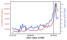
To analyze ETT behaviors, the total time window of observation $W$ is set as 12 months from Nov 14 2017 to Nov 14 2018 and the minimal analytic interval (MAI) $\Delta$ is set as one week. We set $\delta$ from Definition 1 as 1.5 and get all users with ETT behavior in each MAI illustrated in Fig. 4. The red line shows the total number of users who tweet at least once during each MAI, and the blue line shows the percentage of users with ETT behavior. Before September 2018, there are only a few users with ETT behaviors, however, after September the fraction of ETT users grows significantly, and reaches a peak at around the mid October of 2018. To get a reasonable number of ETT users for our experiments, we select a 6-week time period around the 2018 United States mid-term elections held on November 6, 2018. Specifically, our experiments are based on tweets from October 1 to November 14, 2018, partitioned into 6 nearly equal time intervals.

Figure 4: Percentage of users with ETT behavior at each MAI. The largest number exceeds 12000, over 10% of the number of users.

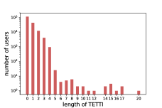
The length of total ETT intervals (TETTI) for each user is calculated and Fig. 5 shows the distribution of users over TETTI lengths. Most users are regular users who never have ETT behavior. Only a few number of users have ETT behaviors frequently. The largest TETTI length within the 54 observation MAIs is 20.

Figure 5: Distribution of users over TETTI length.

V-B Interest Narrowness Analysis

Anomalous users are selected out for each time period by following the framework illustrated in Algorithm 1. The two hyper parameters, $\delta$ and $\lambda$, are set to 1.5 and 1 respectively. Table I shows the fraction of ETT users and the fraction of anomalous users (AU in Table I) over ETT users during each time period.

TABLE I: Percentages of ETT users and Anomalous Users

Time Period	Users Count	ETT (% of Users)	AU (% of ETT)
Oct 1 - 7	52,262	7.54	8.15
Oct 8 - 15	76,935	8.57	8.51
Oct 16 - 23	89,810	10.31	9.38
Oct 24 - 31	122,570	6.14	11.69
Nov 1 - 7	96,858	7.36	11.03
Nov 8 - 14	69,060	8.19	7.92

V-B1 Change of interest narrowness over different time periods

We calculate the interest narrowness for every extreme tweeter at each time period. Fig. 6 shows the distribution of extreme tweeters over interest narrowness value at two time periods: Oct 1 - 7 and Nov 1 - 7.

Figure 6: Extreme tweeters distribution over interest narrowness

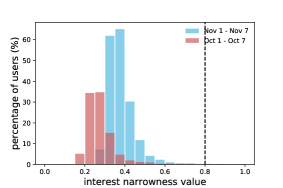
The user distribution shifts to right when time range changes from Oct 1 - 7 to Nov 1 - 7 and more extreme tweeters concentrate on higher narrowness, i.e., extreme tweeters have narrower topic interests during Nov 1 - 7.

V-B2 Analysis of users with extreme interest narrowness

As the black dashed line in Fig. 6 shows, a few users have extremely high interest narrowness, i.e., only $10\%$ of their tweets count number of topics can well represent all their tweets. In order to understand their tweeting behaviors, for each time period, we select users with interest narrowness higher than $80\%$ and dive into their tweets. Many of these users have extremely high narrowness because they have a lot of “null text tweets” where they do not write any of their own words but only mention others. We select out users with more than $80\%$ null text tweets and Table II shows their total tweets count and the number of users mentioned by them during a certain time period.

TABLE II: Users with more than 80% of null text tweets

Time Period	Users Count	Tweets Count	Mentions Counts
Oct 1 - 7	4	459	203
Oct 8 - 15	9	906	1,158
Oct 16 - 23	13	1,956	1,284
Oct 24 - 31	5	2,459	1,058
Nov 1 - 7	4	2,600	3,222
Nov 8 - 14	4	725	129

During Oct 8 - Nov 7, a handful of users contribute many null text tweets and there are a large volume of users mentioned by them. The situation becomes the most extreme during Nov 1 - 7 when four users have 2600 tweets in total, of which more than 80% have no self-written words, and mention more than 3000 distinct users.

V-C User Distribution over Coreness

To analyze the social connectivity between anomalous users and other user categories, we construct the largest subgraphs from the complete social network that satisfying Type-I, Type-II and Type-III connection patterns for each time period. We call them Type-I, Type-II, Type-III social network in the whole experiment section.

V-C1 Type-I Social Network

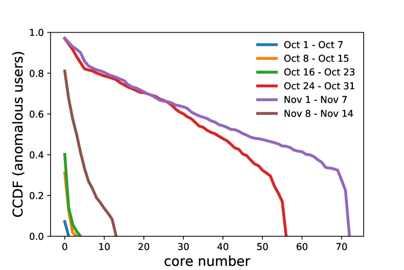
We evaluate the distribution of anomalous users over coreness in Type-I social network at different time periods, and Fig. 7(a) shows the complementary cumulative distribution function (CCDF) of anomalous users. In the first three weeks of October, most users do not interact with each other and more than half of anomalous users have 0 coreness. However, when it is near the American midterm election, i.e., from Oct 24 - Nov 7, the red and purple lines decrease slowly at the beginning and go down quickly at the tail, suggesting that users concentrate on high coreness. There are only around 700 anomalous users at Nov 1 - 7 from Table I, while the largest coreness is 72, which implies extremely strong connections amongst them. However, after the election, the largest coreness dropped to 13, which means that many anomalous users leave hot interaction with others. In addition, the distribution of users tends to be more uniform since the brown line decreases smoothly.

(a) Type I Network

(b) Type II Network

Figure 7: CCDF of anomalous users over coreness.

V-C2 Type-II and III Social Networks

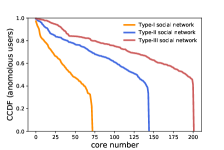
We evaluate the coreness distribution of anomalous users when their ETT- or regular neighbors are included. Fig. 8 shows the CCDF of anomalous users over coreness in three types of networks during Nov 1 - 7. When including first neighbors, the coreness of anomalous users increases dramatically, suggesting that many anomalous users have strong connections with their neighbors. The yellow line reaches bottom before coreness 75, but there are around 70% and 80% of anomalous users with coreness larger than 75 in Type-II and Type-III networks respectively. In addition, the largest coreness increases from 72 to around 140 and 200. However, from Table I, the number of anomalous users is only around 11% of ETTs and less than 0.8% of regular users at Nov 1 - 7. Considering the sizes of these three user categories, the increase of coreness of anomalous users is of less significance. Thus, we conclude that many anomalous users indeed have strong connections with some extreme tweeters or regular users, however, from a holistic view of three categories, interactions amongst anomalous users themselves are stronger than those between anomalous users with ETT users or regular users.

Figure 8: CCDF of anomalous users in three networks during Nov 1 - 7

V-C3 Change of Social Network over Time

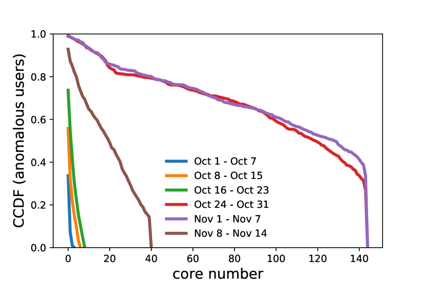
To analyze the dynamic pattern of social networks, we also plot the CCDF of anomalous users for Type-II social networks during all observation periods. As shown in Fig. 7, both Type-I and Type-II networks show the similar trend of changes. At the first three time periods, users do not involve in dense interaction with each other and the lines decrease rapidly at the beginning and reach 0 before 15 coreness. However, during Oct 24 - Nov 7, the lines suddenly and dramatically shift to right and they decrease slowly at first but much faster at the tail, which means that many users interact intensively with each other. However, after midterm election, the lines (brown lines) shift to left and social networks tend to become more silent, but users still have more interactions than normal days, e.g., Oct 1 - 7. In a word, the interaction intensity between users changes over time, especially during important real world events.

V-D Anomalous Group Behavior Pattern

For first three weeks of our observation window, there is no anomalous group formed because anomalous users do not interact heavily during these time intervals. We find an anomalous group in the other three time periods. Table III presents their group coreness of Type-I connection pattern (denoted as Coreness 1) and of Type-II pattern (denoted as Coreness 2), and their common neighbor ratio and diversity ratio in Type-II connection pattern.

TABLE III: Anomalous Groups

Time Period	Coreness 1	Coreness 2	CNR	DR
Oct 24 - 31	56	143	0.37	1.59
Nov 1 - 7	72	144	0.40	0.89
Nov 8 - 14	13	37	0.21	4.62

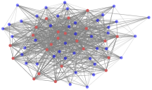
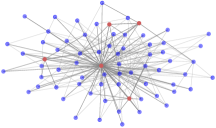
During Nov 1 - 7, as the relatively high CNR and low DR values suggest, the anomalous users in this group (Group I) tend to have similar mention behaviors and they do not interact with many people comparing to their group size. Instead, during Nov 8 - 14, anomalous users in the group (Group II) tend to have diverse behaviors, i.e., they do not interact with others collaboratively and they mention a lot of people. Fig. 9 shows two sample subgraphs satisfying Type-II connection pattern for these two groups. The red nodes denote users from the anomalous group and blue nodes denote extreme tweeters who connect with at least one anomalous user.

(a) Group I

(b) Group II

Figure 9: Sample subgraphs satisfying Type-II connection pattern.

(a) Group I

(b) Group II

Figure 10: Hashtag histogram for anomalous group.

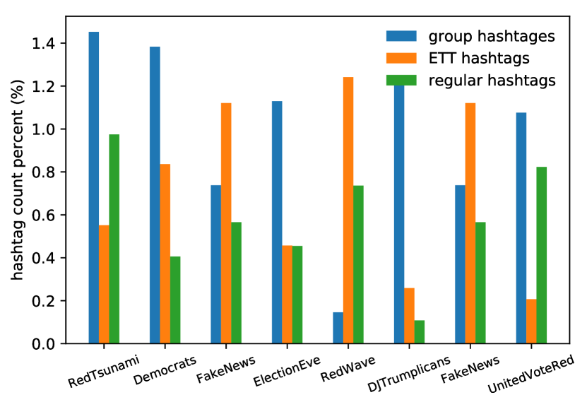
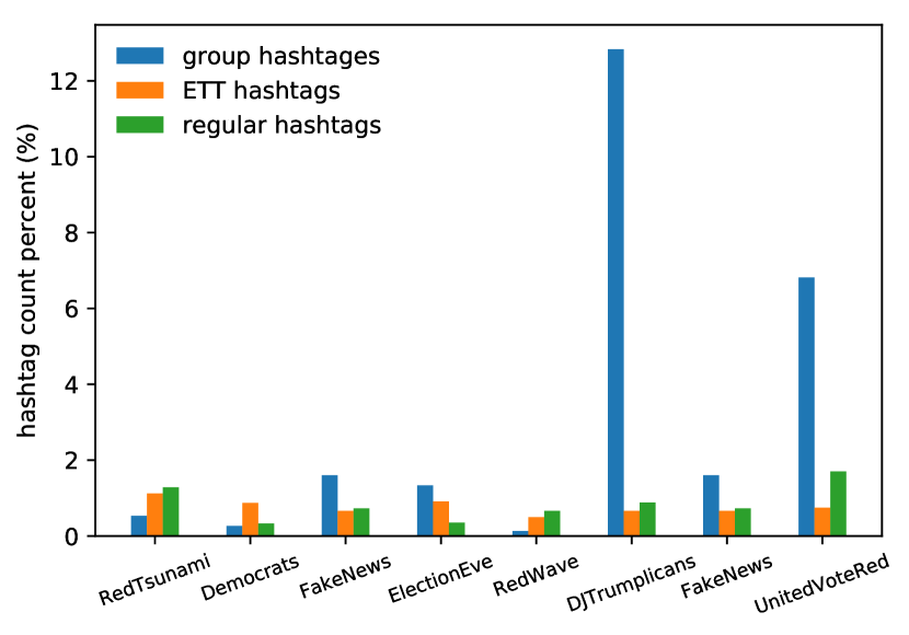
The two anomalous groups show completely different mention behaviors. We collect all hashtags used by members of each group to mention i) regular users (regular hashtags), ii) non-anomalous ETT (ETT hashtags) and iii) each other within group (group hashtags). Fig. 10 shows the count percentages of a same subset of hashtags for the two groups. We calculate the correlation coefficient between counts of group hashtags and ETT hashtags (coef1) and that between counts of group hashtags and regular hashtags (coef2) as shown in Table IV. Besides, the standard deviations (stdev) for group hashtags, ETT hashtags and regular hashtags distributions (stdev1, stdev2, stdev3 respectively in Table IV) are calculated for each group. Note that the stdev presented in this section is standardized by the percentage of hashtag counts.

TABLE IV: Statistics of Hashtag Distributions

	coef1	coef2	stdev1	stdev2	stdev3
Group I	0.81	0.77	0.004	0.003	0.002
Group II	0.31	0.10	0.024	0.008	0.004

For Group I, it has similar intra-group and inter-group hashtag usage behaviors as two correlation coefficients indicate, and all the three distributions have very low stdev, indicating a uniform use of hashtags. For Group II, however, the low coefficients suggest that this group may have different hashtag uses when they mention amongst group members versus mention other categories. In addition, the distribution of group hashtags (blue bars in Fig. 10) has much higher stdev than the other two distributions (yellow and green bars in Fig. 10). It indicates that some hashtags (e.g., DJTrumplicans or UnitedVoteRed) are used disproportionately often when members of Group II interact amongst themselves. However, when they mention other categories of users, their hashtag distribution is more uniform, i.e., the conversation covers broader topics.

During the first three time periods in our observation window, only one or two users in Group II are ETT users. However, since Oct 24, most members of Group II show sustained hyperactivity and high interest narrowness, i.e., they are anomalous users during the other three time periods. Table V presents their group coreness in Type-I connection pattern and the stdev of three hashtag distributions. For each time period, this group shows highly-skewed hashtag usage within group, but broader interests outside it.

TABLE V: Behaviors of Group II During Different Time Periods

Time Period	Coreness	stdev1	stdev2	stdev3
Oct 24 - 31	54	0.040	0.004	0.005
Nov 1 - 7	62	0.015	0.003	0.003

VI Conclusion

Our experimental results confirm that our user stratification strategy successfully brings out the unusual behavior of the extreme tweeters. The strategy itself is fairly generic and can be applied to any social media platform. In terms of results, we find that the highly-connected group we call “anomalous” indeed exhibits a “clannish” behavior because of their strong and narrowly-scoped within-group interactions that markedly differs from their across-group behavior. The fact that their “reach” increases with time, especially leading up to the US mid-term elections, suggests that the group has strong political beliefs and forms a strong trust network of its own that establishes contact with a high number of users but carefully controls content outside the group. Similarly, the “anomalous” aspect of their behavior dramatically comes into play two weeks before the elections, suggesting a motivation to reinforce each others’ beliefs and perhaps an intention to influence others in their mention network.

Our future work will elaborate this case study to uncover other characteristics of these user groups and their interactions. We will conduct a larger comparative study across more diverse time periods, a larger cross-section of users, and user behavior in different hashtag communities. We will also investigate more computationally efficient methods of finding interest narrowness, and user stratification.

References

- [1] J. I. Alvarez-Hamelin, L. Dall’Asta, A. Barrat, and A. Vespignani. Large scale networks fingerprinting and visualization using the k-core decomposition. In Adv. in Neural Info. Proc. Syst., pages 41–50, 2006.
- [2] C. A. Bail. Combining natural language processing and network analysis to examine how advocacy organizations stimulate conversation on social media. Proc. of the National Academy of Sciences, 113(42):11823–11828, 2016.
- [3] E. J. Candès and B. Recht. Exact matrix completion via convex optimization. Found. of Comput. Mathematics, 9(6):717, 2009.
- [4] S. N. Dorogovtsev, A. V. Goltsev, and J. F. F. Mendes. K-core organization of complex networks. Phys. Rev. Letters, 96(4):40601, 2006.
- [5] P. A. Grabowicz, L. M. Aiello, V. M. Eguiluz, and A. Jaimes. Distinguishing topical and social groups based on common identity and bond theory. In Proc. of the 6th ACM Int. Conf. on Web search and data mining, pages 627–636. ACM, 2013.
- [6] N. Halko, P.-G. Martinsson, and J. A. Tropp. Finding structure with randomness: Probabilistic algorithms for constructing approximate matrix decompositions. SIAM review, 53(2):217–288, 2011.
- [7] Q. Huang, V. K. Singh, and P. K. Atrey. Cyber bullying detection using social and textual analysis. In Proc. of the 3rd Int. Workshop on Socially-Aware Multimedia, pages 3–6. ACM, 2014.
- [8] J. Jang and S.-H. Myaeng. Discovering dedicators with topic-based semantic social networks. In Proc. of the 7th Int. AAAI Conf. on Weblogs and Social Media, 2013.
- [9] F. T. O’Donovan, C. Fournelle, S. Gaffigan, O. Brdiczka, J. Shen, J. Liu, and K. E. Moore. Characterizing user behavior and information propagation on a social multimedia network. In 2013 IEEE Int. Conf. on Multimedia and Expo Workshops, pages 1–6. IEEE, 2013.
- [10] H. Shaban. Twitter reveals its daily active user numbers for the first time. Washington Post, Feb. 2019.
- [11] T. Tuna, E. Akbas, A. Aksoy, M. A. Canbaz, U. Karabiyik, B. Gonen, and R. Aygun. User characterization for online social networks. Social Network Analysis and Mining, 6(1):104, 2016.
- [12] J. Ugander, L. Backstrom, C. Marlow, and J. Kleinberg. Structural diversity in social contagion. Proc. of the National Academy of Sciences, 109(16):5962–5966, 2012.