Drug-Drug Adverse Effect Prediction
with Graph Co-Attention

Abstract.

Complex or co-existing diseases are commonly treated using drug combinations, which can lead to higher risk of adverse side effects. The detection of polypharmacy side effects is usually done in Phase IV clinical trials, but there are still plenty which remain undiscovered when the drugs are put on the market. Such accidents have been affecting an increasing proportion of the population (15% in the US now) and it is thus of high interest to be able to predict the potential side effects as early as possible. Systematic combinatorial screening of possible drug-drug interactions (DDI) is challenging and expensive. However, the recent significant increases in data availability from pharmaceutical research and development efforts offer a novel paradigm for recovering relevant insights for DDI prediction. Accordingly, several recent approaches focus on curating massive DDI datasets (with millions of examples) and training machine learning models on them. Here we propose a neural network architecture able to set state-of-the-art results on this task—using the type of the side-effect and the molecular structure of the drugs alone—by leveraging a co-attentional mechanism. In particular, we show the importance of integrating joint information from the drug pairs early on when learning each drug’s representation.

1. Introduction

Diseases are often caused by complex biological processes which cannot be treated by individual drugs and thus introduce the need for concurrent use of multiple medications. Similarly, drug combinations are needed when patients suffer from multiple medical conditions. However, the downside of such treatment (commonly referred to as polypharmacy) is that it increases the risk of adverse side effects, caused by the chemical-physical incompatibility of the drugs. Such drug-drug interactions (DDIs) have become a serious issue in recent times, affecting nearly 15% of the US population (ED et al., 2015), with treatment costs exceeding $177 billion/year (Ernst and Grizzle, 2001).

Detection of polypharmacy side effects remains a challenging task to this day: systematic combinatorial screening is expensive and, while the search for such side effects is usually done during clinical testing, the small scale of the trials and the rarity of adverse DDI means that many adverse drug reactions (ADRs) are unknown when the drugs reach the market. Moreover, the immense cost of designing a drug makes it desirable to be able to predict ADRs as early as possible in the pipeline.

In this work, we propose the use of deep learning to ameliorate this problem. One of deep learning’s main advantages is the ability to perform automated feature extraction from raw data. This means that, provided the existence of sufficiently large datasets, models can now be developed without depending on manually engineered features, which are expensive to obtain and require expert domain knowledge (Goodfellow et al., 2016). In this work, we leverage such a large dataset (Tatonetti et al., 2012), consisting of $\sim$4.5M examples of (drug, drug, interaction) tuples, to demonstrate that these models are indeed viable in the DDI domain.

By looking at the chemical structures of the drug pairs, our model learns drug representations which incorporate joint drug-drug information. We then predict whether a drug-drug pair would cause side effects and what their types would be. Our method outperforms previous state-of-the-art models in terms of predictive power, while using just the molecular structure of the drugs. It thus allows for the method to be applied to novel drug combinations, as well as permitting the detection to be performed at the preclinical phase rather than in the drug discovery phase, leveraging clinical records.

Our approach paves the way to a new and promising direction in analysing polypharmacy side effects with machine learning, that is in principle applicable to any kind of interaction discovery task between structured inputs (such as molecules), especially under availability of large quantities of labelled examples.

Figure 1. An overview of the binary (left) and multi-label (right) drug-drug interaction (DDI) task. In both cases, two drugs (represented as their molecular structures) are provided to the model in order to predict existence or absence of adverse interactions. For binary classification, the DDI predictor is also given a particular side effect as input, and is required to specifically predict existence or absence of it. For multi-label classification, the DDI predictor simultaneously predicts existence or absence of all side-effects under consideration.

2. Related work

Our work finds itself at the intersection of two domains: computational methods for prediction of side effects caused by DDI and neural networks for graph-structured data. As such, a review of related advances in each area will be presented here.

As manually examining drug combinations and their possible side effects cannot be done exhaustively, computational methods were first developed to identify the drug pairs which create a response higher than the additive response they would cause if they did not interact (Ryall and Tan, 2015). This was previously done by framing the task as a binary classification problem and designing machine learning models (naïve Bayes, logistic regression, support vector machines) which predict the probability of a DDI, using the measurement of cell viability (Huang et al., 2014; Sun et al., 2015; Zitnik and Zupan, 2016; Chen et al., 2016; Shi et al., 2017). Other related approaches considered dose-effect curves (Bansal et al., 2014; Takeda et al., 2017) or synergy and antagonism (Lewis et al., 2015).

An alternative way of approaching the task is provided by models which use the assumption that drugs with similar features are more likely to interact (Gottlieb et al., 2012; Vilar et al., 2012; Huang et al., 2014; Li et al., 2015; Žitnik and Zupan, 2015; Sun et al., 2015; Li et al., 2017). Using features such as the chemicals’ structures, individual drug side effects and interaction profile fingerprints, the models use unsupervised or semi-supervised techniques (clustering, label propagation) in order to find DDIs. Alternatively, restricted Boltzmann machines and matrix factorization were used to combine different types of similarities by learning latent representations (Cao et al., 2015; Wang and Zeng, 2013).

However, all these methods are limited to either providing the likelihood of a DDI (but not its type if one exists), or lack applicability in inductive settings. Decagon (Zitnik et al., 2018) and the Multitask Dyadic Prediction in (Jin et al., 2017) are two methods which overcome these challenges, and are thus going to be used as baselines against which our work will be compared. Multitask Dyadic Prediction is a proximal gradient method which uses substructure fingerprints to construct the drug feature representations. Similarly to our work, it has access only to the chemical structure of the drug.

Decagon, on the other hand, improves predictive power further by including additional relational information with protein targets of interest. Specifically, Decagon leverages this information by applying a graph convolutional neural network architecture over a graph corresponding to the interactions between pairs of drugs, pairs of proteins and drug-protein pairs, treating discovery of novel DDIs as a link prediction task in the graph. While the protein-related auxiliary information is highly beneficial for the algorithm to use, it could also be expensive to obtain.

Compared to previous methods, our contribution is a model which learns a robust representation of drugs by leveraging joint information early on in the learning process. This allows it to bring an improvement in terms of predictive power, while maintaining an inductive setup where the model indicates the types of the possible side effects by just looking at chemical structure of the drugs.

Our model builds up on a large existing body of work in graph convolutional networks (Bruna et al., 2013; Defferrard et al., 2016; Kipf and Welling, 2016; Gilmer et al., 2017; Veličković et al., 2018), that have substantially advanced the state-of-the-art in many tasks requiring graph-structured input processing (such as the chemical representation (Gilmer et al., 2017; De Cao and Kipf, 2018; You et al., 2018) of the drugs leveraged here). Furthermore, we build up on work proposing co-attention (Lu et al., 2016; Deac et al., 2018) as a mechanism to allow for individual set-structured datasets (such as nodes in multimodal graphs) to interact. Overall, these (and related) techniques correspond to one of the latest major challenges of machine learning (Bronstein et al., 2017; Hamilton et al., 2017; Battaglia et al., 2018), with transformative potential across a wide spectrum of potential applications (not only limited to the biochemical domain).

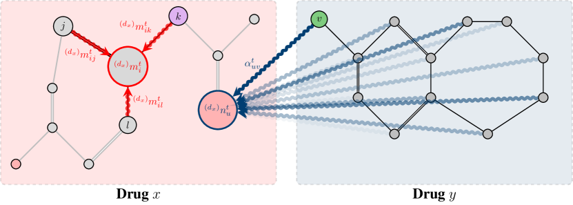
Figure 2. The illustration of a single step of message passing (computing the inner message, ${}^{(d_{x})}m_{i}^{t}$), and co-attention (computing the outer message ${}^{(d_{x})}n_{u}^{t}$) on two nodes ($i$ and $u$) of drug $x$.

3. Architecture

In this section, we will present the main building blocks used within our architecture for drug-drug interaction prediction. This will span a discussion of the way the input to the model is encoded, followed by an overview of the individual computational steps of the model. Lastly, we will specify the loss functions optimised by the models.

3.1. Inputs

The drugs, $d_{x}$, are represented as graphs consisting of atoms, $a^{(d_{x})}_{i}$ as nodes, and bonds between those atoms $\left(a^{(d_{x})}_{i},a^{(d_{x})}_{j}\right)$ as edges. For each atom, the following input features are recorded: the atom number, the number of hydrogen atoms attached to this atom, and the atomic charge. For each bond, a discrete bond type (e.g. single, double etc.) is encoded as a learnable input edge vector, $e_{ij}^{(d_{x})}$. The side effects, $se_{z}$, are one-hot encoded from a set of 964 side effects.

The input to our model varies depending on whether we are performing binary classification for a given side effect, or multi-label classification for all side effects at once:

• For binary classification (Figure 1 (Left)), the input to our model is a triplet of two drugs and a side effect $(d_{x},d_{y},se_{z})$, requiring a binary decision on whether drugs $x$ and $y$ adversely interact to cause side effect $z$.

• For multi-label classification (Figure 1 (Right)), the input to our model is a pair of two drugs $(d_{x},d_{y})$, requiring 964 simultaneous binary decisions on whether drugs $x$ and $y$ adversely interact to cause each of the considered side effects. Note that, in terms of learning pressure, this model requires more robust joint representations of pairs of drugs—as they need to be useful for all side-effect predictions at once.

In both cases, the model returns a score associated with the likelihood of a particular side effect occurring (higher scores implying larger likelihoods). This score can then be appropriately thresholded to obtain a viable classifier.

3.2. Message passing

Within each of the two drugs separately, our model applies a series of message passing (Gilmer et al., 2017) layers. Herein, nodes are allowed to send arbitrary vector messages to each other along the edges of the graph, and each node then aggregates all the messages sent to it.

Let ${}^{(d_{x})}h_{i}^{t}$ denote the features of atom $i$ of drug $x$, at time step $t$. Specially, initially these are set to projected input features, i.e.:

(1) $${}^{(d_{x})}h_{i}^{0}=f_{i}\left(a_{i}^{(d_{x})}\right)$$

where $f_{i}$ is a small multilayer perceptron (MLP) neural network. In all our experiments, this MLP (and all subsequently referenced MLPs and projections) projects its input to 32 features.

Considering atoms $i$ and $j$ of drug $x$, connected by a bond with edge vector $e_{ij}^{(d_{x})}$, we start by computing the message, ${}^{(d_{x})}m_{ij}^{t}$, sent along the edge $j\rightarrow i$. The message takes into account both the features of node $j$ and the features of the edge between $i$ and $j$:

(2) $$^{(d_{x})}m_{ij}^{t}=f_{e}^{t}\left(e_{ij}^{(d_{x})}\right)\odot f_{v}^{t}\left({}^{(d_{x})}h_{j}^{t-1}\right)$$

where $f_{e}^{t}$ and $f_{v}^{t}$ are small MLPs, and $\odot$ is elementwise vector-vector multiplication.

Afterwards, every atom $i$ aggregates the messages sent to it via summation. This results in an internal message for atom $i$, ${}^{(d_{x})}m_{i}^{t}$:

(3) $${}^{(d_{x})}m_{i}^{t}=\sum_{\forall j\in N(i)}{}^{(d_{x})}m_{ij}^{t}$$

where the neighbourhood, $N(i)$, defines the set of atoms linked to $i$ by an edge.

3.3. Co-attention

Message passing provides a robust mechanism for encoding within-drug representations of atoms. For learning an appropriate joint drug-drug representation, however, we allow atoms to interact across drug boundaries via a co-attentional mechanism (Deac et al., 2018).

Consider two atoms, $i$ and $j$, of drugs $x$ and $y$, respectively. Let their features at time step $t$ be ${}^{(d_{x})}h_{i}^{t}$ and ${}^{(d_{y})}h_{j}^{t}$, just as before. For every such pair, we compute an attentional coefficient, $\alpha_{ij}^{t}$ using a simplified version of the Transformer (Vaswani et al., 2017) attention mechanism:

(4) $$\alpha_{ij}^{t}=\mathrm{softmax}_{j}\left(\left<{\bf W}_{k}^{t}{}^{(d_{x})}h_{i}^{t-1},{\bf W}_{k}^{t}{}^{(d_{y})}h_{j}^{t-1}\right>\right)$$

where ${\bf W}_{k}^{t}$ is a learnable projection matrix, $\left<\cdot,\cdot\right>$ is the inner product, and the softmax is taken across all nodes $j$ from the second drug. The coefficients $\alpha_{ij}^{t}$ may be interpreted as the importance of atom $j$’s features to atom $i$.

These coefficients are then used to compute an outer message for atom $i$ of drug $x$, ${}^{(d_{x})}n_{i}^{t}$, expressed as a linear combination (weighted by $\alpha_{ij}^{t}$) of all (projected) atom features from drug $y$:

(5) $$^{(d_{x})}n_{i}^{t}=\sum_{\forall j\in d_{y}}\alpha_{ij}^{t}\cdot{\bf W}_{v}^{t}{}^{(d_{y})}h_{j}^{t-1}$$

where ${\bf W}_{v}^{t}$ is a learnable projection matrix.

It was shown recently that multi-head attention can stabilise the learning process, as well as learn information at different conceptual levels (Veličković et al., 2018; Qiu et al., 2018). As such, the mechanism of Equation 5 is independently replicated across $K$ attention heads (we chose $K=8$), and the resulting vectors are concatenated and MLP-transformed to provide the final outer message for each atom.

(6) $$^{(d_{x})}n_{i}^{t}=f_{o}^{t}\left(\operatorname*{\scalebox{1.0}[1.5]{$\parallel$}}_{k=1}^{K}\sum_{\forall j\in d_{y}}{}^{(k)}\alpha_{ij}^{t}\cdot{}^{(k)}{\bf W}_{v}^{t}{}^{(d_{y})}h_{j}^{t-1}\right)$$

where $f_{o}^{t}$ is a small MLP and $\|$ is featurewise vector concatenation.

The computation of Equations 4–6 is replicated analogously for outer messages from drug $x$ to atoms of drug $y$.

We have also attempted to use other popular attention mechanisms for computing the $\alpha_{ij}^{t}$ values—such as the original Transformer (Vaswani et al., 2017), GAT-like (Veličković et al., 2018) and tanh (Bahdanau et al., 2014) attention—finding them to yield weaker performance than the approach outlined here.

A single step of message passing and co-attention, as used by our model, is illustrated by Figure 2.

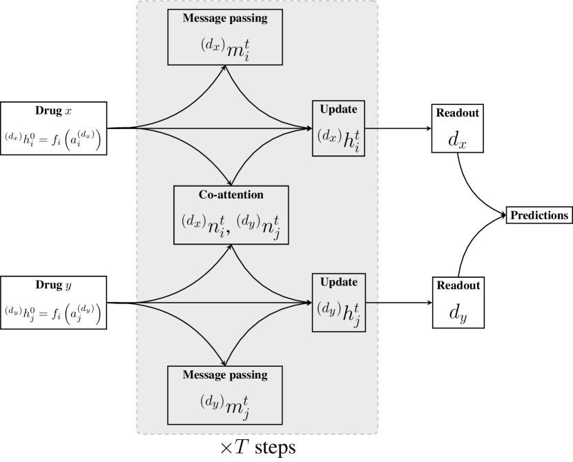
Figure 3. A high-level overview of our DDI model. The next-level features of atom $i$ of drug $x$, ${}^{(d_{x})}h_{i}^{t}$, are derived by combining its input features, ${}^{(d_{x})}h_{i}^{t-1}$, its inner message, ${}^{(d_{x})}m_{i}^{t}$, computed using message passing, and its outer message, ${}^{(d_{x})}n_{i}^{t}$, computed using co-attention over the second drug, $d_{y}$.

3.4. Update function

Once the inner messages, ${}^{(d_{x})}m_{i}^{t}$ (obtained through message passing), as well as the outer messages, ${}^{(d_{x})}n_{i}^{t}$ (obtained through co-attention) are computed for every atom $i$ of each of the two drugs ($d_{x}$/$d_{y})$, we use them to derive the next-level features, ${}^{(d_{x})}h_{i}^{t}$, for each atom.

At each step, this is done by aggregating (via summation) the previous features (representing a skip connection (He et al., 2016)), the inner messages and outer messages, followed by layer normalisation (Ba et al., 2016):

(7) $$^{(d_{x})}h_{i}^{t}=\mathrm{LayerNorm}\left({}^{(d_{x})}h_{i}^{t-1}+{}^{(d_{x})}m_{i}^{t}+{}^{(d_{x})}n_{i}^{t}\right)$$

The operations of Equations 2–7 are then repeated for $T$ propagation steps—here, we set $T=3$. Refer to Figure 3 for a complete visualisation of our architecture.

As will be demonstrated in the Results section, using co-attention to enable the model to propagate the information between two drugs from the beginning—thus learning a joint representation of the drugs—valuably contributes to the predictive power of the model.

3.5. Readout and Scoring

As we’re making predictions on the level of entire drug-drug pairs, we need to compress individual atom representations into drug-level representations. In order to obtain the drug-level vectors $d_{x}$, we apply a simple summation of its constituent atom feature vectors after the final layer (i.e. after $T$ propagation steps have been applied):

(8) $$d_{x}=\sum_{\forall j\in d_{x}}f_{r}\left({}^{(d_{x})}h_{j}^{T}\right)$$

where $f_{r}$ is a small MLP.

Once the drug vectors are computed for both $d_{x}$ and $d_{y}$, these can be used to make predictions on side effects—and the exact setup varies depending on the type of classification.

3.5.1. Binary classification

In the binary classification case, the side effect vector $se_{z}$ is provided as input. We then leverage a scoring function $f$ similar to the one used by Yoon et al. (Yoon et al., 2016) to express the likelihood of this side effect occuring:

(9) $$f(d_{x},d_{y},se_{z})=\mathinner{\!\left\lVert{\bf M}_{h}d_{x}+se_{z}-{\bf M}_{t}d_{y}\right\rVert}^{2}_{2}+\mathinner{\!\left\lVert{\bf M}_{h}d_{y}+se_{z}-{\bf M}_{t}d_{x}\right\rVert}^{2}_{2}$$

where $\|\cdot\|_{2}$ is the $L_{2}$ norm, and ${\bf M}_{h}$ and ${\bf M}_{t}$ represent the head node and tail node space mapping matrices, respectively.

The model is then trained end-to-end with gradient descent to optimise a margin-based ranking loss:

(10) $$\mathcal{L}=\sum_{d_{x},d_{y},se_{z}}\sum_{\tilde{d_{x}},\tilde{d_{y}},se_{z}}\max(0,\gamma-f(d_{x},d_{y},se_{z})-f(\tilde{d_{x}},\tilde{d_{y}},se_{z})))$$

where $(d_{x},d_{y})$ is a drug-drug pair exhibiting side effect $se_{z}$, and $(\tilde{d_{x}},\tilde{d_{y}})$ is a drug-drug pair not exhibiting it. $\gamma>0$ is the margin hyperparameter.

3.5.2. Multi-label classification

Here, all side effects are predicted simultaneously, and accordingly we define a prediction layer, param-etrised by a learnable weight matrix ${\bf W}_{p}$ and bias $b_{p}$. This layer consumes the concatenation of the two drug vectors and projects it into a score for each of the 964 side effects. These scores are then converted into probabilities, $y_{xy}^{z}$, of each side effect, $z$, occurring between drugs $x$ and $y$ using the logistic sigmoid nonlinearity, $\sigma$, applied elementwise:

(11) $$y_{xy}^{z}=\sigma\left({\bf W}_{p}[d_{x}\|d_{y}]+b_{p}\right)_{z}$$

We can then once again train the model end-to-end with gradient descent, using binary cross-entropy against the ground truth value, $\hat{y}_{xy}^{z}$ (which is a binary label indicating whether side effect $z$ actually occurs between drugs $x$ and $y$). The loss function is as follows:

(12) $$\mathcal{L}_{BCE}=\sum_{d_{x},d_{y},z}\hat{y}_{xy}^{z}\log{y_{xy}^{z}}+\left(1-\hat{y}_{xy}^{z}\right)\log{\left(1-y_{xy}^{z}\right)}$$

4. Dataset and Preprocessing

The drug-drug interaction data was chosen to be in agreement with the dataset used by Decagon (Zitnik et al., 2018). It is obtained through filtering the TWOSIDES side-effect dataset (Tatonetti et al., 2012), which consists of associations which cannot be clearly attributed to either drug alone (that is, those side-effects reported for any individual drug in the OFFSIDE dataset (Tatonetti et al., 2012)) and it comprises 964 polypharmacy side-effect types that occurred in at least 500 drug pairs.

The data format used within the dataset is: (1) The compound ID of drug 1; (2) The compound ID of drug 2; (3) Side effect concept identifier; (4) Side effect name. In order to obtain the drug-related features, we look up the compound IDs in the PubChem database. This provides us with the molecular structure of each drug:

• Atoms, including type, charge and coordinates for each atom;

• Bonds, including type and style for each bond;

• SMILES string.

In order to compensate for the fact that TWOSIDES contains only positive samples, appropriate negative sampling is performed for the binary classification task:

• During training, tuples $(\tilde{d_{x}},\tilde{d_{y}},se_{z})$, where $\tilde{d_{x}}$ and $se_{z}$ are chosen from the dataset and $\tilde{d_{y}}$ is chosen at random from the set of drugs different from $d_{y}$ in the true samples $(\tilde{d_{x}},d_{y},se_{z})$.

• During validation and testing, we simply randomly sample two distinct drugs which do not appear in the positive dataset.

The full dataset consists of 4,576,785 positive examples. As we aim to sample a balanced number of positive and negative examples, the overall dataset size for training our model is 9,153,570 examples.

5. Experimental setup

As previously described, our model consists of $T=3$ propagation blocks (featuring a message-passing layer followed by a co-attentional layer with $K=8$ attention heads). Each block computes 32 intermediate features. To further regularise the model, dropout (Srivastava et al., 2014) with $p=0.2$ is applied to the output of every intermediate layer. The model is initialised using Xavier initialisation (Glorot and Bengio, 2010) and trained on mini-batches of 200 drug-drug pairs, using the Adam SGD optimiser (Kingma and Ba, 2014) for 30 epochs. The learning rate after $t$ iterations, $\eta_{t}$, is derived using an exponentially decaying schedule:

(13) $$\eta_{t}=0.001\cdot 0.96^{t\cdot 10^{-6}}$$

We will refer to this model as MHCADDI (multi-head co-attentive drug-drug interactions), and MHCADDI-ML for multi-label classification. We compare our method with the following baselines:

• The work of Jin et al. (Jin et al., 2017) (to be referred to as Drug-Fingerpri-nts), where binary classification is performed through analys-ing the molecular fingerprints of drugs.

• Decagon (Zitnik et al., 2018), where drug-protein interactions and protein-protein interactions are considered in as additional inputs to the model, and the entire interaction graph is simultaneously processed by a graph convolutional network.

• We also report the results of all the baselines used by Decagon, such as the RESCAL (Nickel et al., 2011) and DEDICOM (Papalexakis et al., 2017) tensor decomposition methods and DeepWalk (Perozzi et al., 2014).

In addition, we perform detailed ablation studies to stress the importance of various components of MHCADDI. Specifically, the following baselines are also evaluated:

• An architecture (to be referred to as MPNN-Concat) where the drug representations are learnt separately, solely using internal message passing. The side effect probability is then computed by concatenating the individual drug representations. This serves to demonstrate the importance of jointly learning the drug embeddings (by e.g. co-attention).

• An architecture (to be referred to as Late-Outer) where the outer messages are only considered at the end of the node updating procedure. Each propagation step $t$ of the MPNN function creates “clusters” with information from neighbouring atoms within the same drug at a distance of at most $t$ hops away. The outer messages are then computed at different granularity levels and integrated at the end of the pipeline. Similarly as before, this serves to demonstrate the importance of simultaneously performing internal and external feature extraction.

• An architecture (to be referred to as CADDI) where there is only $K=1$ attention head.

We omit comparisons with traditional machine learning baselines (such as support vector machines or random forests) as prior work (Jin et al., 2017) has already found them to be significantly underperforming compared to neural network approaches on this task.

Table 1. Comparative evaluation results after stratified 10-fold crossvalidation.

	AUROC
Drug-Fingerprints (Jin et al., 2017)	$0.744$
RESCAL (Nickel et al., 2011)	0.693
DEDICOM (Papalexakis et al., 2017)	0.705
DeepWalk (Perozzi et al., 2014)	0.761
Concatenated features (Zitnik et al., 2018)	0.793
Decagon (Zitnik et al., 2018)	$0.872$
MHCADDI (ours)	$\bf 0.882$
MHCADDI-ML (ours)	$0.819$

Table 2. Ablation study for various aspects of the MHCADDI model.

	AUROC
MPNN-Concat	$0.661$
Late-Outer	$0.724$
CADDI	$0.778$
MHCADDI	$\bf 0.882$

Table 3. Top-5 and bottom-5 side effects by AUROC values.

Highest
Side effect	AUROC
Tooth impacted	$0.903$
Nasal polyp	$0.902$
Cluster headache	$0.900$
Balantis	$0.892$
Dysphemia	$0.889$

Lowest
Side effect	AUROC
Neonatal respiratory distress syndrome	$0.670$
Aspergillosis	$0.683$
Obstructive uropathy	$0.690$
Icterus	$0.712$
HIV disease	$0.712$

6. Results

6.1. Quantitative Results

We perform stratified 10-fold crossvalidation on the derived dataset to evaluate our models and compare them against previously published baselines. For each model, we report the area under the receiver operating characteristic (ROC) curve averaged across the 10 folds. The results of our study may be found in Tables 1–2.

From this study, we may conclude that learning joint drug-drug representations by simultaneously combining internal message-passing layers and co-attention between drugs is a highly beneficial approach, consistently outperforming the strong baselines considered here (even when additional data sources are used, as in the case of Decagon). Furthermore, through observing the comparisons between several variants of our architecture, more detailed conclusions easily follow:

• The fact that all our co-attentive architectures outperformed MPNN-Concat implies that it is beneficial to learn drug-drug representations jointly rather than separately.

• Furthermore, the outperformance of Late-Outer by (MH)CA-DDI further demonstrates that it is useful to provide the cross-modal information earlier in the learning pipeline.

• Lastly, the comparative evaluation of MHCADDI against CADDI further shows the benefit of inferring multiple mechanisms of drug-drug interaction simultaneously, rather than anticipating only one.

Finally, we can observe that, despite the additional learning challenges present when doing multi-label classification (in the case of MHCADDI-ML), our jointly learned representations are still competitive with all other baselines. In particular, our method significantly outperforms Drug-Fingerprints—which also uses a multi-label objective.

As an additional ablation study, similarly to the analysis performed by Decagon (Zitnik et al., 2018), for one testing fold we stratified the predictions of our model across all side effects, computing side effect-level AUROC values. These values are given for five of the best- and worst- performing side effects in 3. There is a slight correpondence to the performance of Decagon—with Icterus appearing as one of their worst-performing side effects and a different polyp appearing as one of their best-performing ones. Overall, we do not find that our distribution of per-side-effect AUROC values deviates from the mean value any more substantially than what was reported for Decagon. This implies that our model does not drastically sacrifice performance on some side-effects—at least, not compared to the prior baseline methods which use auxiliary data sources.

6.2. Qualitative Results

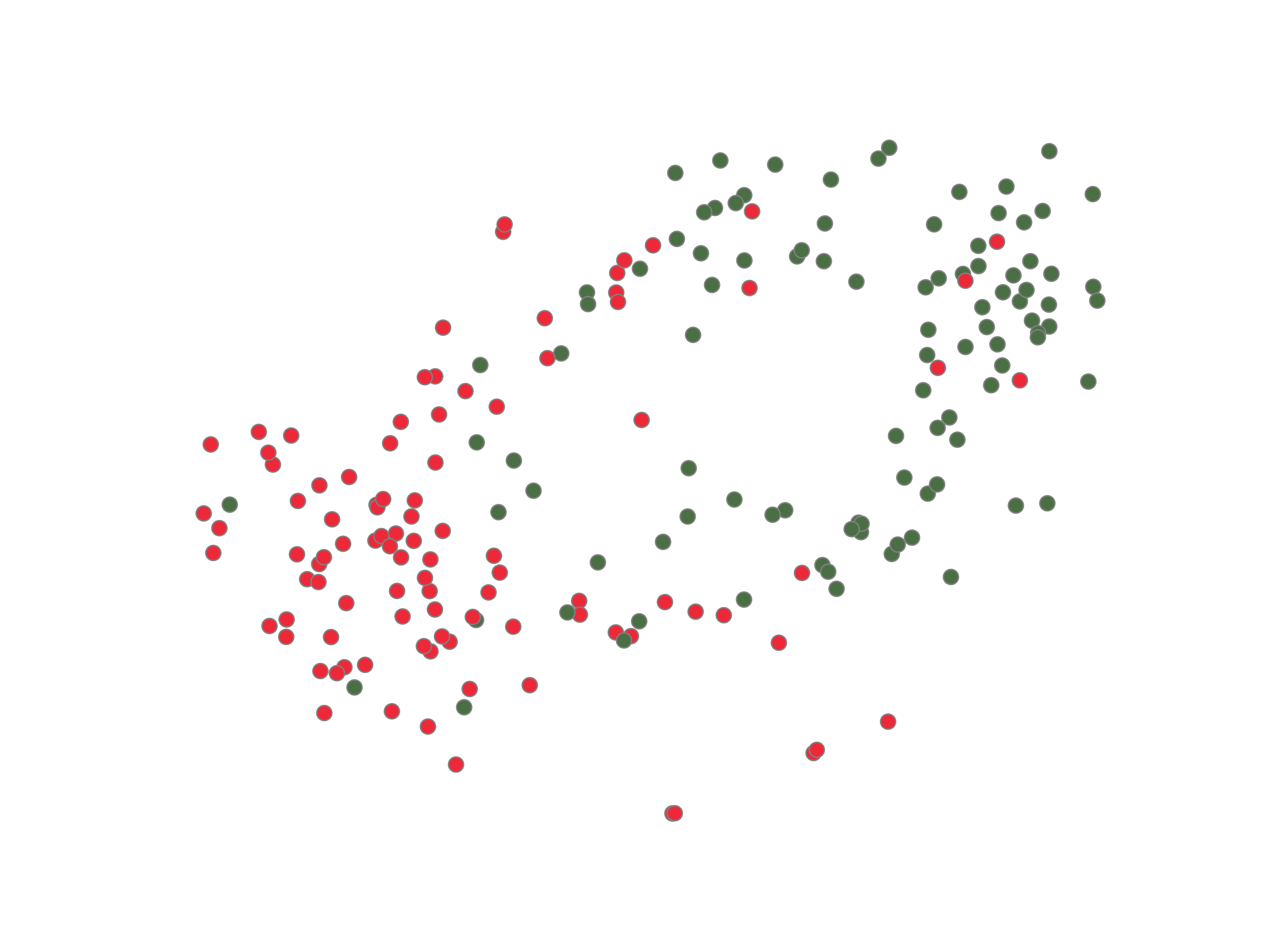
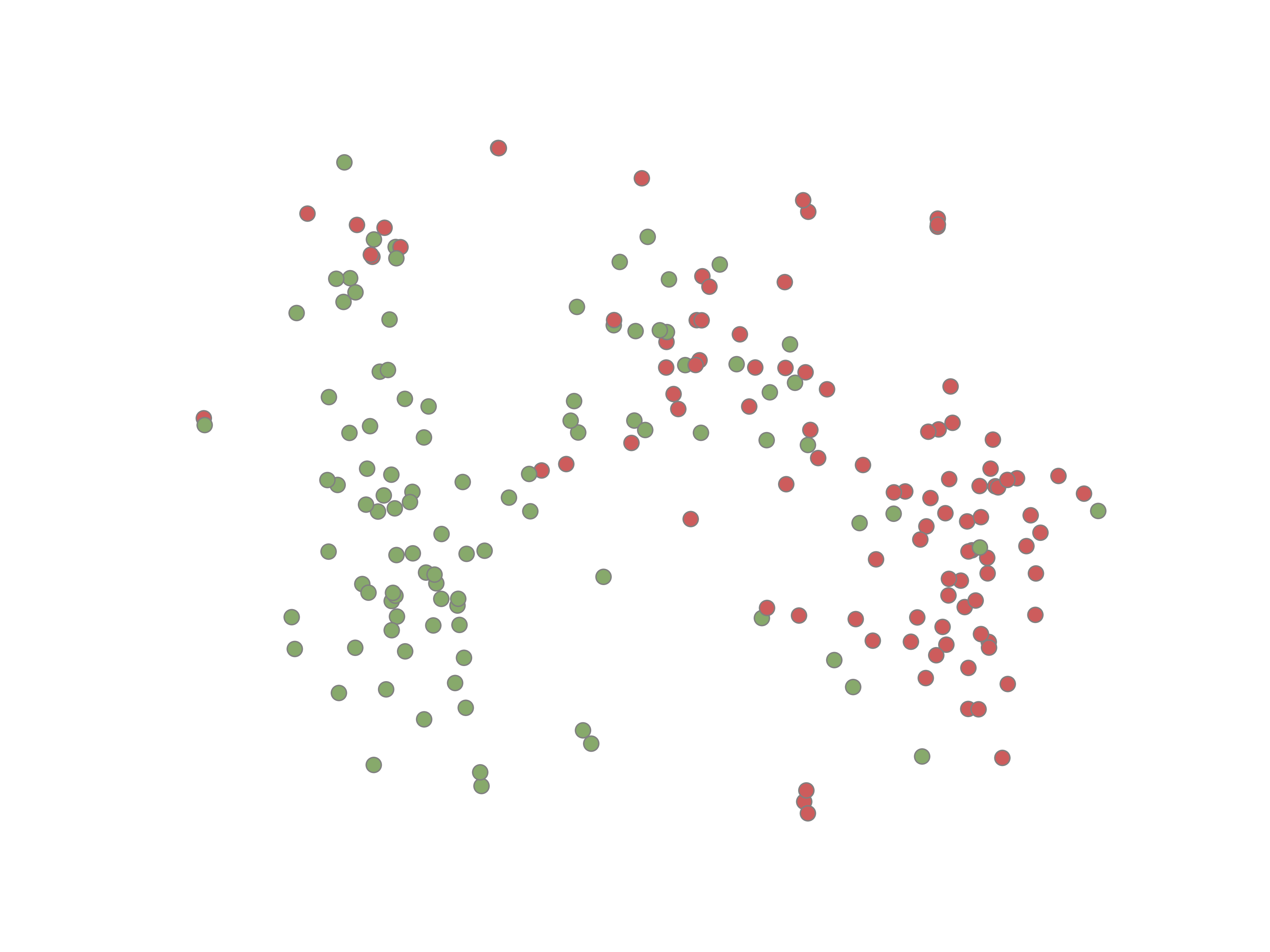
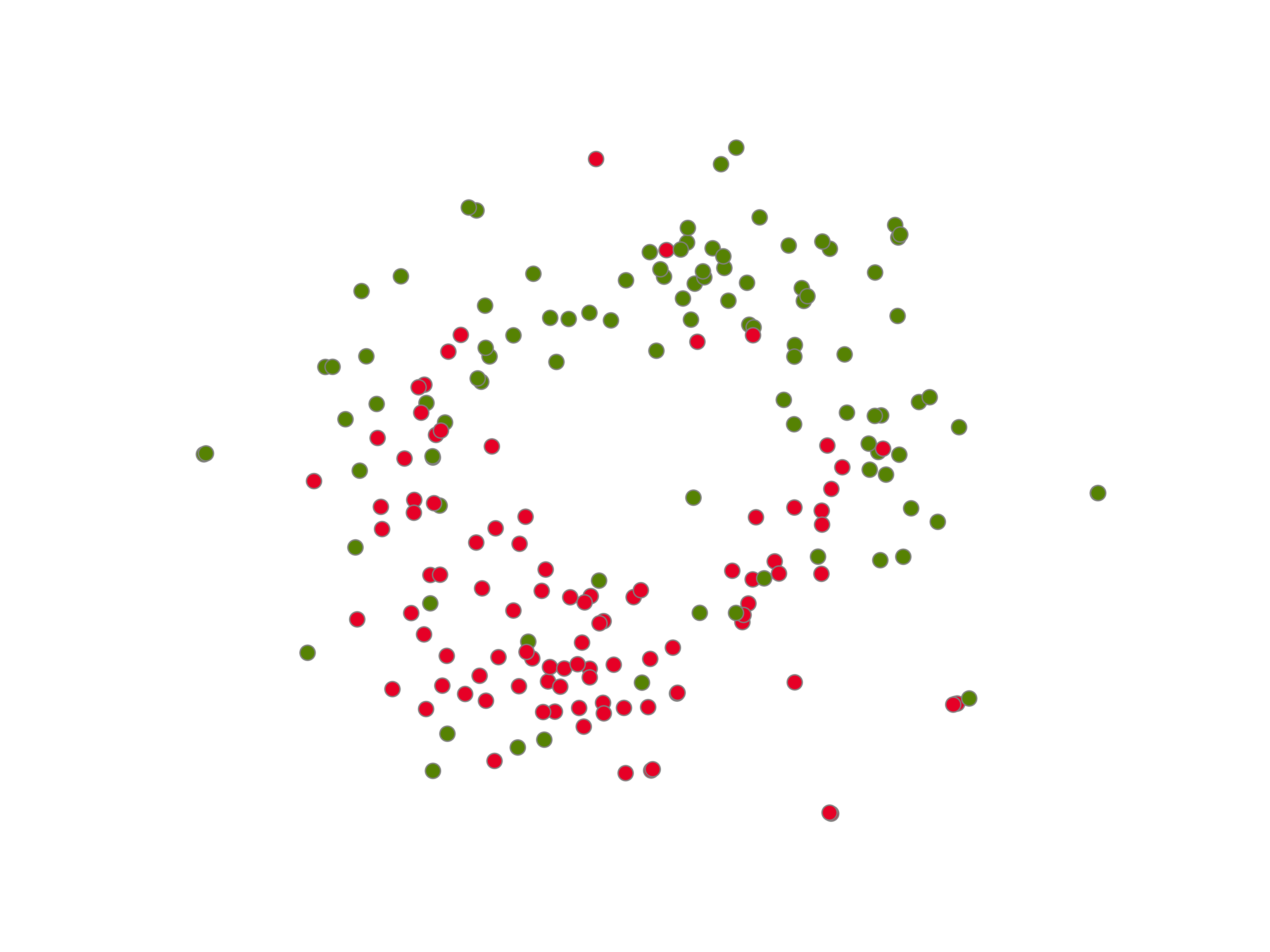
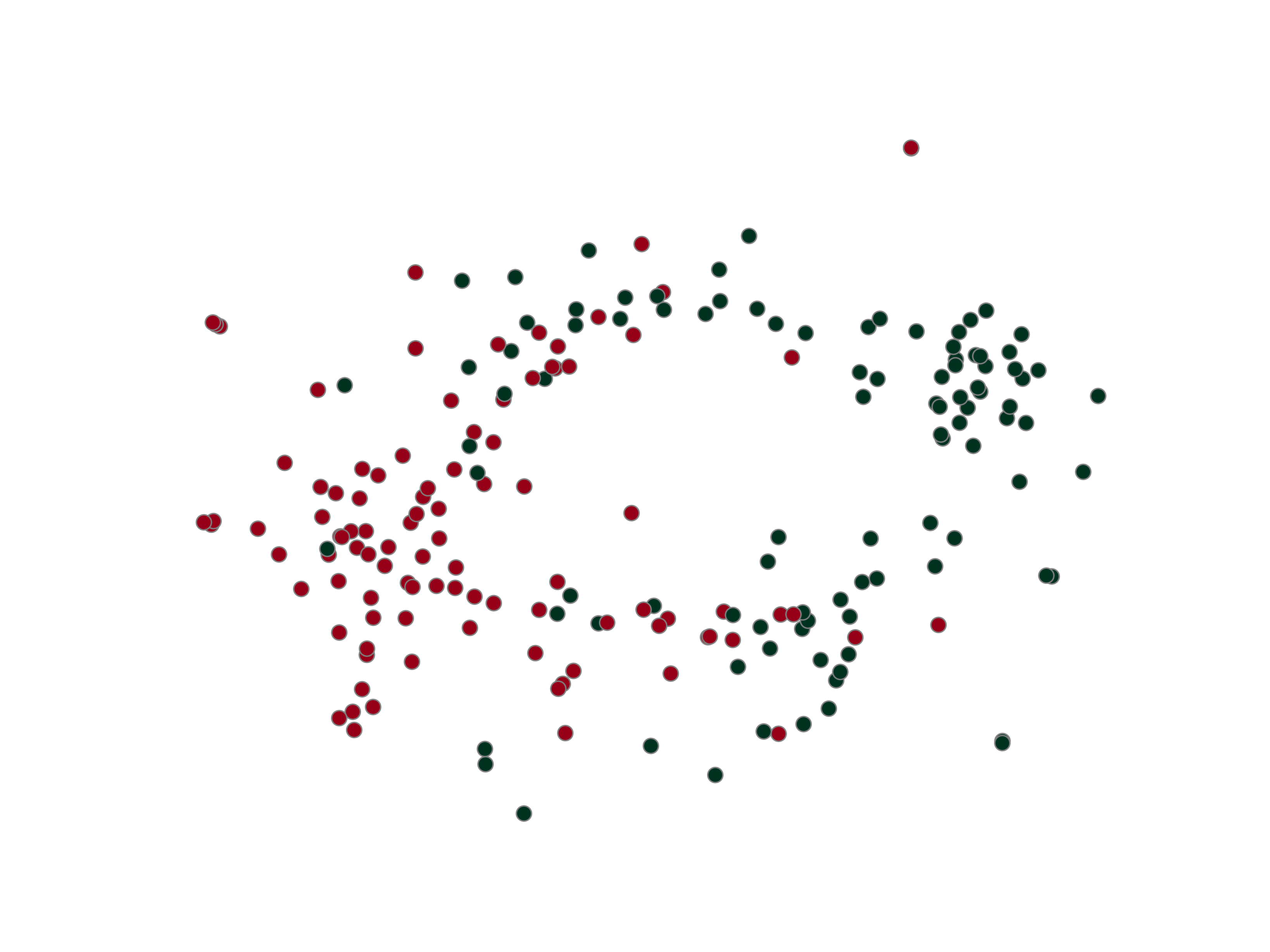
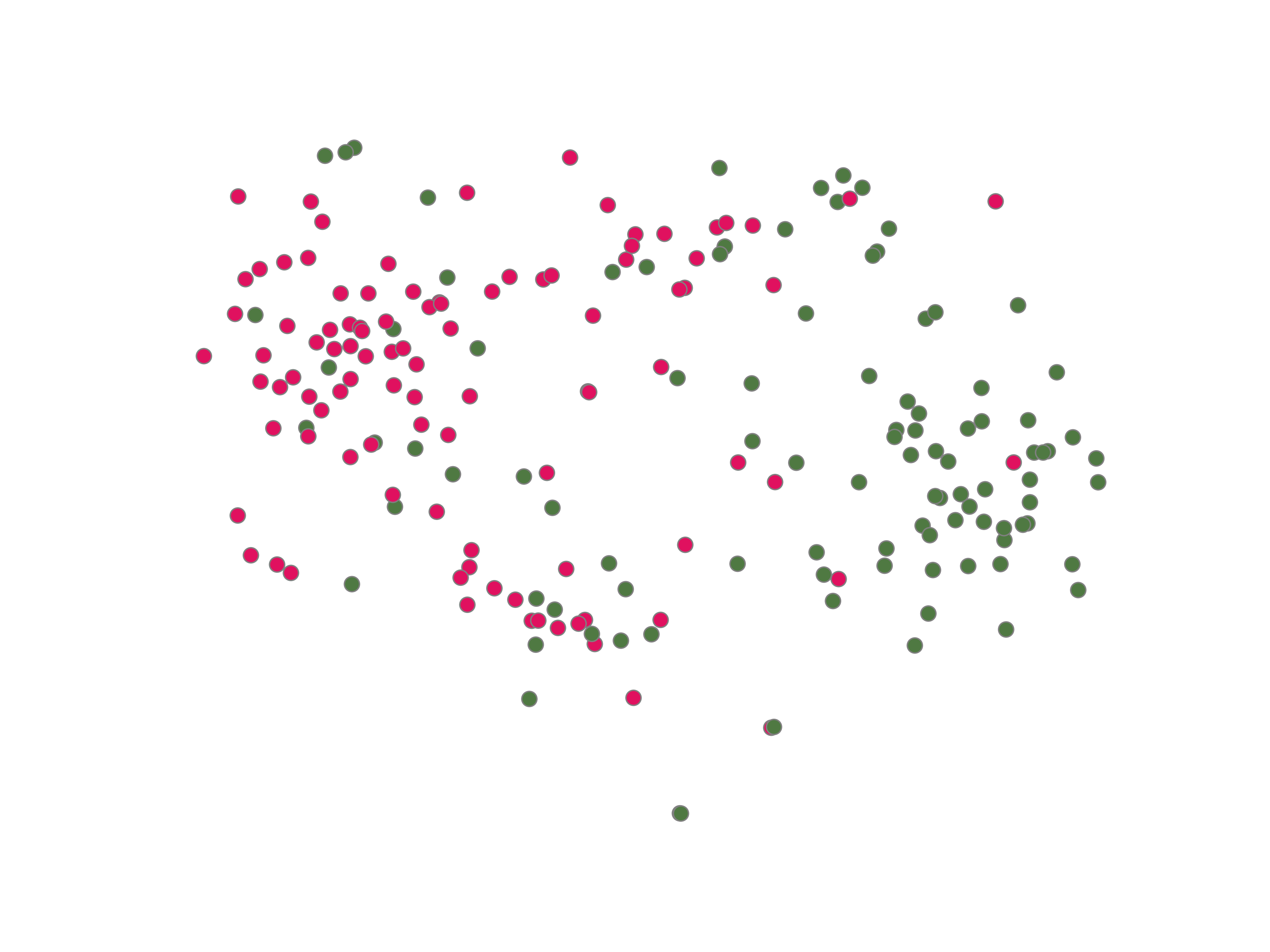
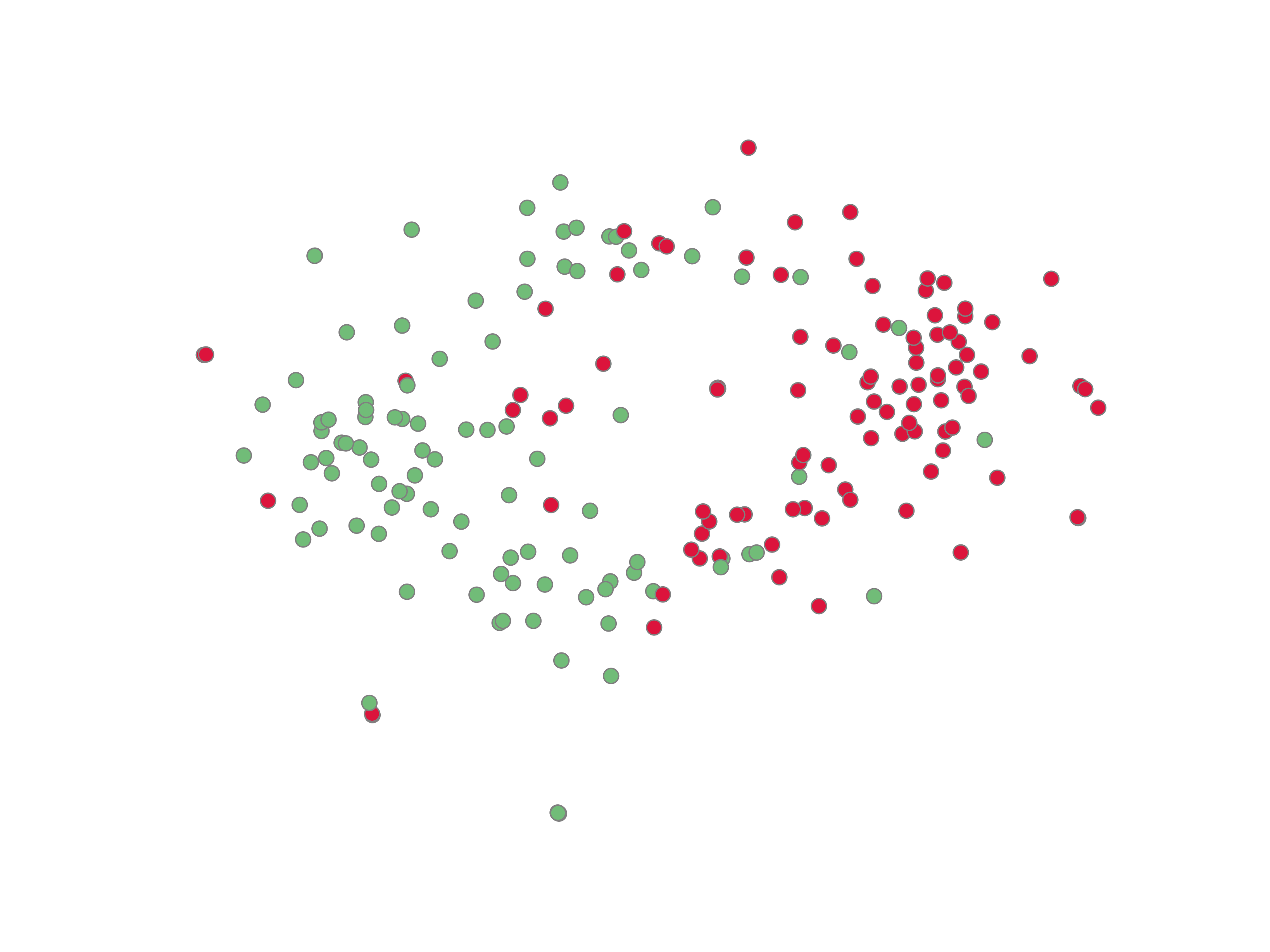
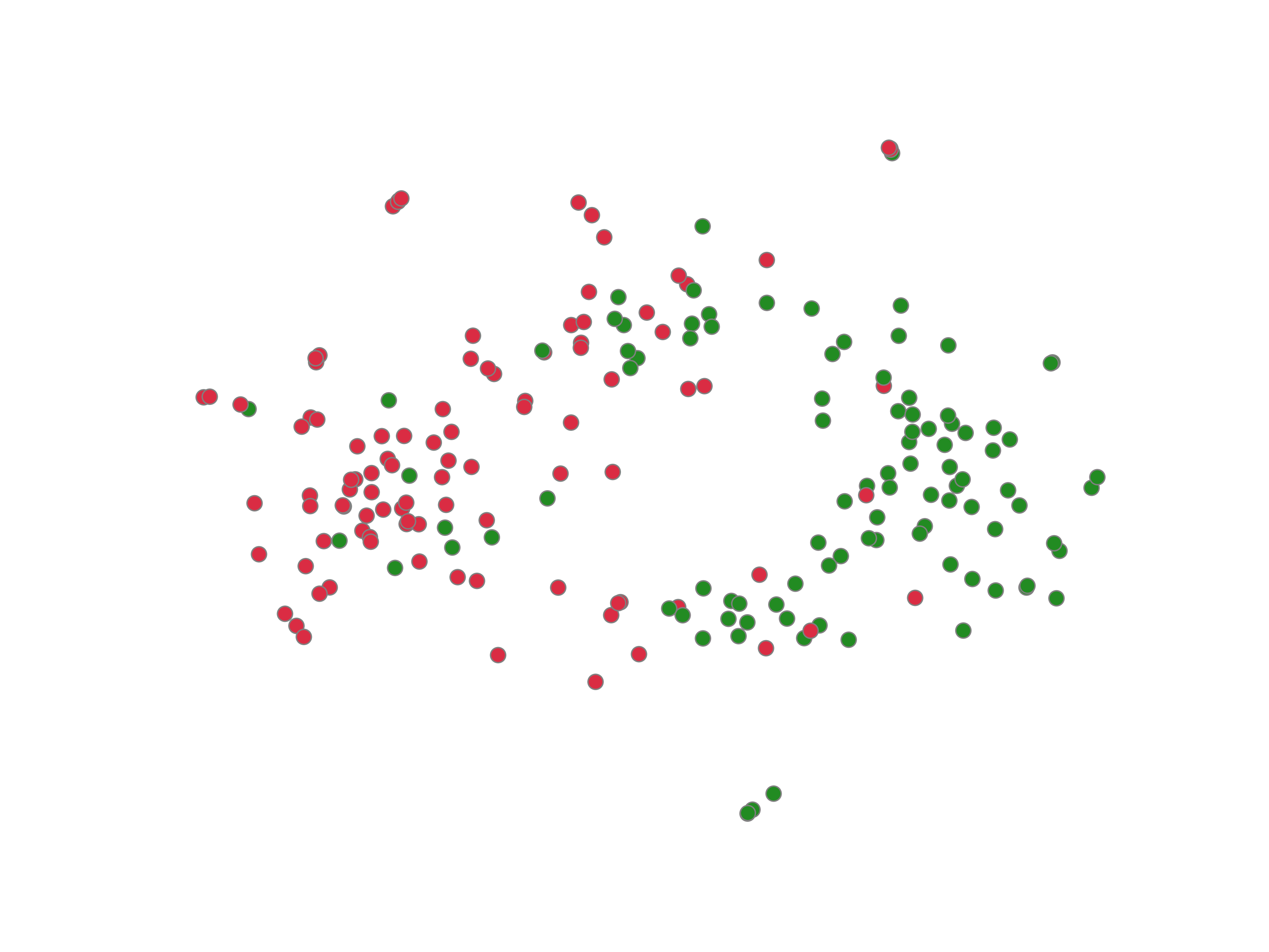
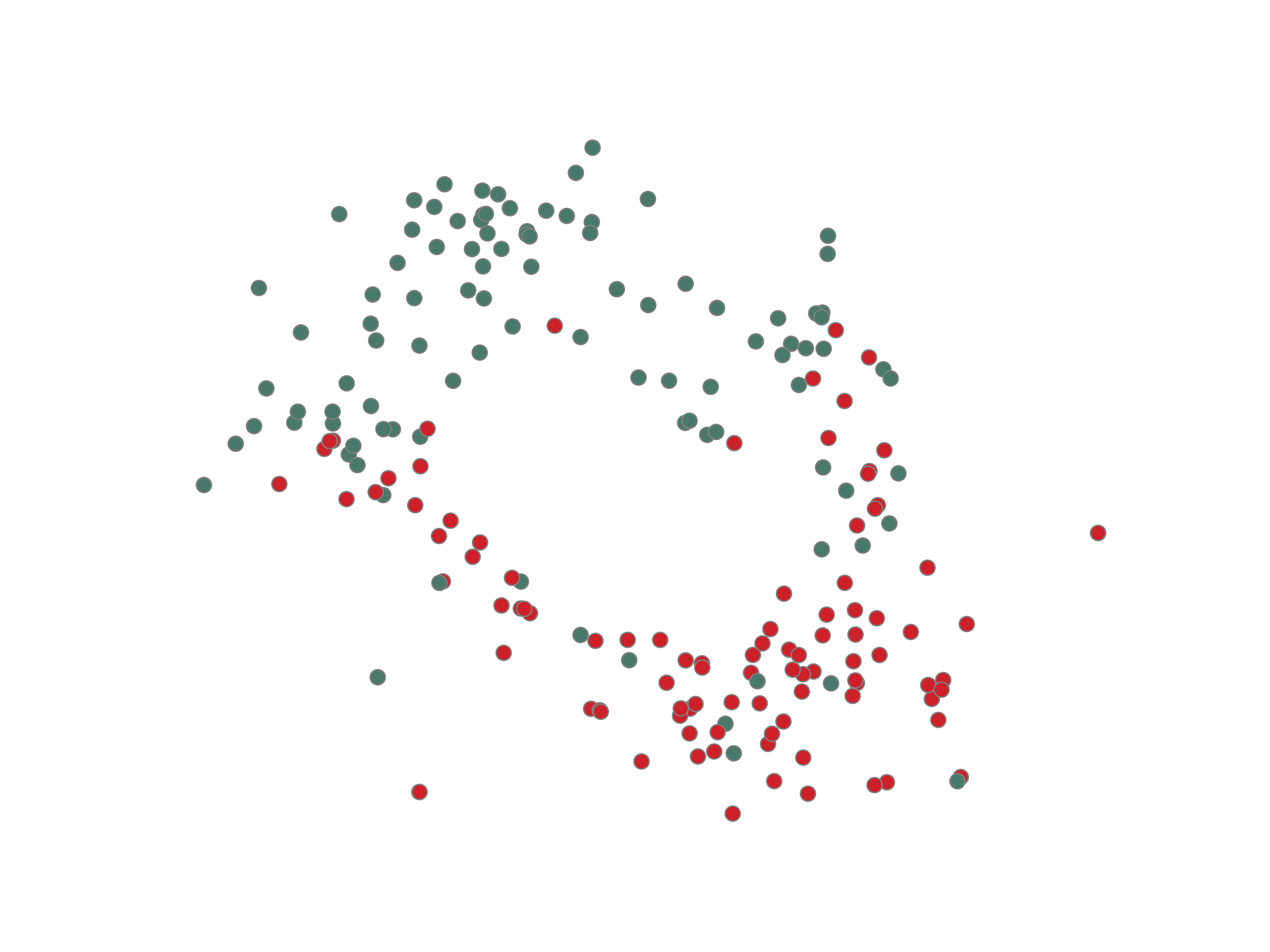
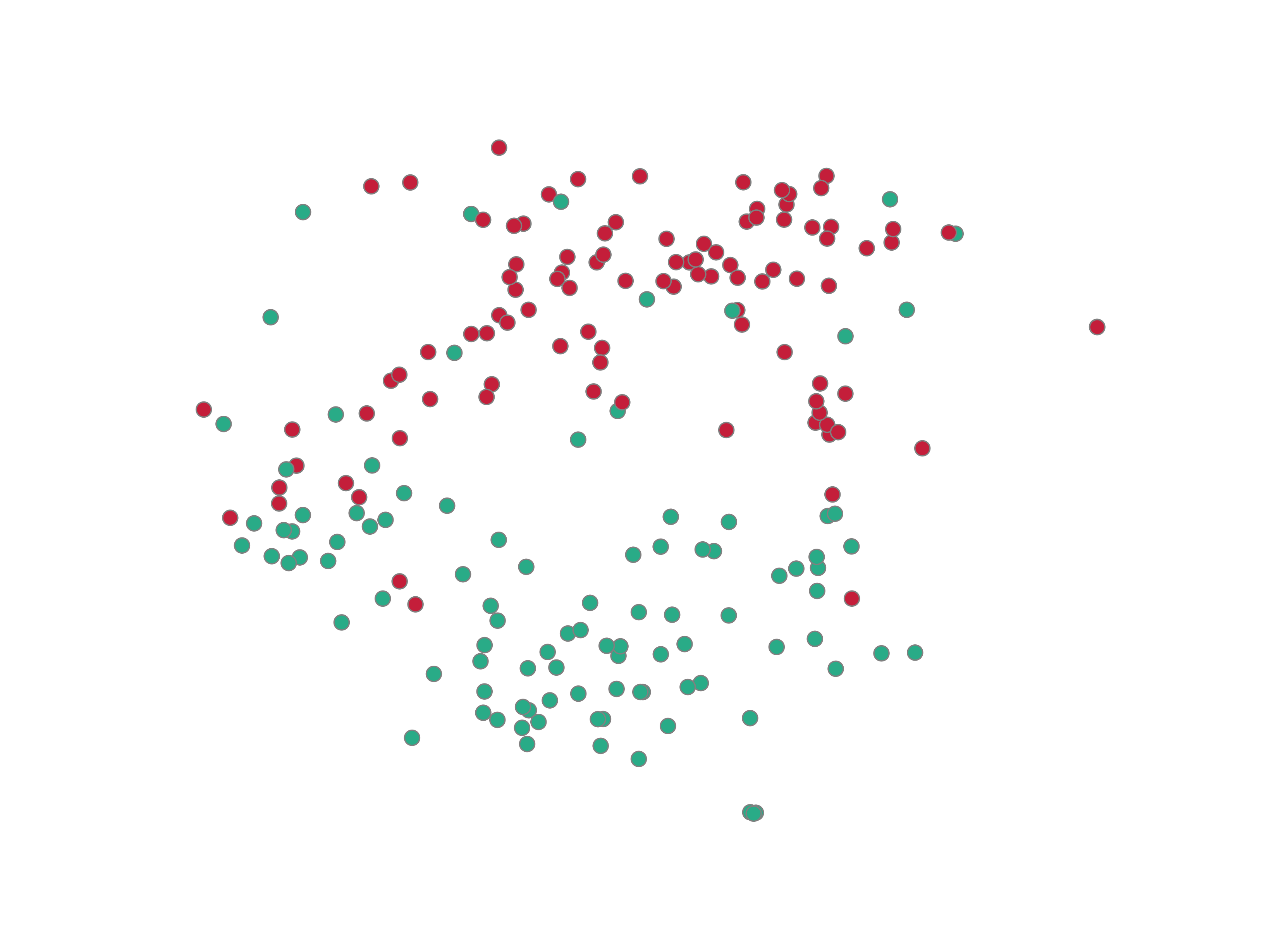
Figure 4. t-SNE projections of 200 learnt drug-drug representations, across 9 side-effects. Each side effect is colour-coded with a shade of red for positive drug-drug pairs and a shade of green for negative pairs.

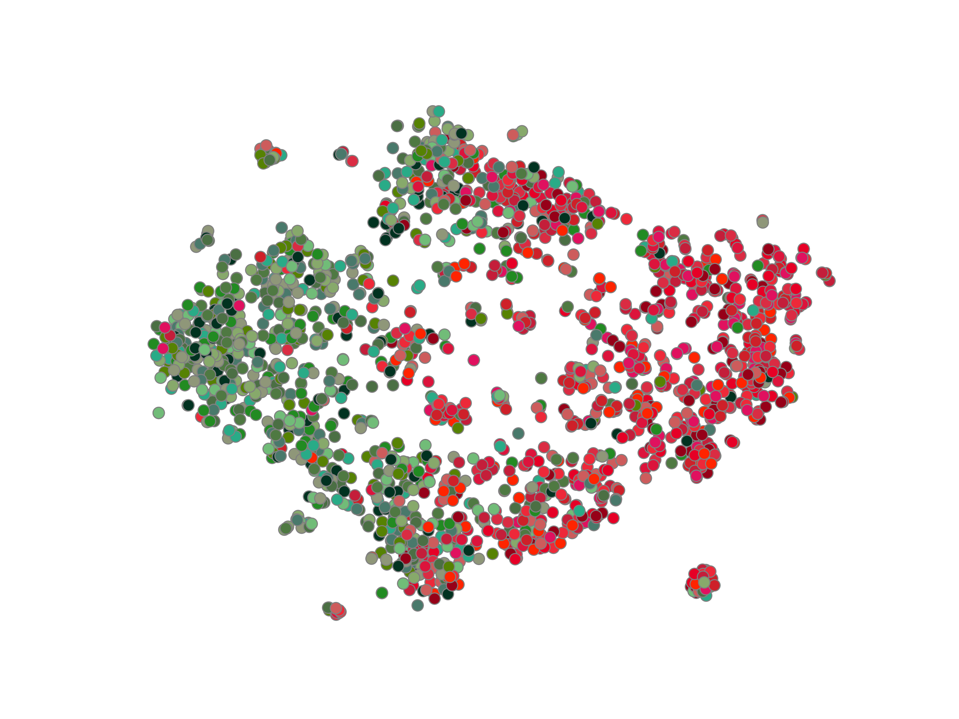
Figure 5. t-SNE projection of 2000 learnt drug-drug representations, sampled to cover 10 side effects. Each side effect is colour-coded with a shade of red for positive drug-drug pairs and a shade of green for negative drug-drug pairs.

The effectiveness of the learnt joint representations may be investigated qualitatively as well, and to that end, we have devised a controlled visualisation experiment. Our objective is to investigate the distribution of learnt drug-drug embeddings with respect to individual side effects.

We start with a pre-trained MHCADDI model. For each side effect in a sample of 10, we have randomly sampled 100 drug-drug pairs exhibiting this side effect, and 100 drug-drug pairs not exhibiting it (both unseen by the model during training). For these pairs, we derived their embeddings, and projected them into two dimensions using t-SNE (Maaten and Hinton, 2008).

The visualised embeddings may be seen in Figure 4 for individual side-effects, and Figure 5 for a combined plot. These plots demonstrate that, across a single side-effect, there is a discernible clustering in the projected 2D space of drug-drug interactions. Furthermore, the combined plot demonstrates that strongly side-effect inducing drug-drug pairs tend to be clustered together, and away from the pairs that do not induce side-effects.

7. Conclusions

In this work, we have presented a graph neural network architecture which sets state-of-the-art results for predicting the possible polypharmacy side effects of drug combinations, using solely the molecular structure information of drug pairs. By performing message passing within each drug, as well as co-attending over the other drug’s structure, we demonstrated the power of integrating joint drug-drug information during the representation learning phase for individual drugs. Future directions could include applying such cross-modal architectures to predicting interactions in different kinds of networks (such as language or social) where the components of different networks interact with each other.

Appendix A Hyperparameters

In the interests of reproducibility, in this supplementary material we detail all the hyperparameters used for training and evaluating our MHCADDI model described above.

For each atom, its features $a_{i}^{(d_{x})}$ are obtained by concatenating the specified input features with a learnable embedding (unique to each atom) of 32 dimensions.

The input node projection function, $f_{i}$, is a single-layer MLP with no bias:

(14) $$f_{i}(x)={\bf W}_{f_{i}}x$$

computing 32 features, followed by dropout with $p=0.2$.

The learnable edge embeddings, $e_{ij}^{(d_{x})}$, are of 32 features, and dropout with $p=0.2$ is immediately applied to them once retrieved.

The node projection MLP for message passing, $f_{v}^{t}$, is a single-layer MLP with no bias:

(15) $$f_{v}^{t}(x)={\bf W}_{f_{v}^{t}}x$$

computing 32 features, followed by dropout with $p=0.2$.

The edge projection MLP for message passing, $f_{e}^{t}$, is a two-layer MLP with leaky ReLU (Maas et al., 2013) activations:

(16) $$f_{e}^{t}(x)=\text{LeakyReLU}\left({\bf W}_{f_{e}^{t}}^{2}\text{LeakyReLU}\left({\bf W}_{f_{e}^{t}}^{1}x+b_{f_{e}^{t}}^{1}\right)+b_{f_{e}^{t}}^{2}\right)$$

Both layers compute 32 features, and dropout with $p=0.2$ is applied to both of their outputs.

The key/value projection matrices, ${\bf W}_{k}^{t}$ and ${\bf W}_{v}^{t}$, of each attention head, compute 32 features each.

The outer message MLP for co-attention, $f_{o}^{t}$, is a single-layer MLP with the leaky ReLU activation:

(17) $$f_{o}^{t}(x)=\text{LeakyReLU}\left({\bf W}_{f_{o}^{t}}x+b_{f_{o}^{t}}\right)$$

computing 32 features, followed by dropout with $p=0.2$.

The readout projection MLP, $f_{r}$, is a single-layer MLP with the leaky ReLU activation:

(18) $$f_{r}(x)=\text{LeakyReLU}\left({\bf W}_{f_{r}}x+b_{f_{r}}\right)$$

The head node and tail node mapping matrices, ${\bf M}_{h}$ and ${\bf M}_{t}$ (used within the computation of side effect likelihoods), compute 32 features each.

The margin hyperparameter $\gamma$ has been set to $\gamma=1$.

References

- (1)
- Ba et al. (2016) Jimmy Lei Ba, Jamie Ryan Kiros, and Geoffrey E Hinton. 2016. Layer normalization. arXiv preprint arXiv:1607.06450 (2016).
- Bahdanau et al. (2014) Dzmitry Bahdanau, Kyunghyun Cho, and Yoshua Bengio. 2014. Neural machine translation by jointly learning to align and translate. arXiv preprint arXiv:1409.0473 (2014).
- Bansal et al. (2014) Mukesh Bansal, Jichen Yang, Charles Karan, Michael P Menden, James C Costello, Hao Tang, Guanghua Xiao, Yajuan Li, Jeffrey Allen, Rui Zhong, et al. 2014. A community computational challenge to predict the activity of pairs of compounds. Nature biotechnology 32, 12 (2014), 1213.
- Battaglia et al. (2018) Peter W Battaglia, Jessica B Hamrick, Victor Bapst, Alvaro Sanchez-Gonzalez, Vinicius Zambaldi, Mateusz Malinowski, Andrea Tacchetti, David Raposo, Adam Santoro, Ryan Faulkner, et al. 2018. Relational inductive biases, deep learning, and graph networks. arXiv preprint arXiv:1806.01261 (2018).
- Bronstein et al. (2017) Michael M Bronstein, Joan Bruna, Yann LeCun, Arthur Szlam, and Pierre Vandergheynst. 2017. Geometric deep learning: going beyond euclidean data. IEEE Signal Processing Magazine 34, 4 (2017), 18–42.
- Bruna et al. (2013) Joan Bruna, Wojciech Zaremba, Arthur Szlam, and Yann LeCun. 2013. Spectral networks and locally connected networks on graphs. arXiv preprint arXiv:1312.6203 (2013).
- Cao et al. (2015) D-S Cao, N Xiao, Y-J Li, W-B Zeng, Y-Z Liang, A-P Lu, Q-S Xu, and AF Chen. 2015. Integrating multiple evidence sources to predict adverse drug reactions based on a systems pharmacology model. CPT: pharmacometrics & systems pharmacology 4, 9 (2015), 498–506.
- Chen et al. (2016) Di Chen, Huamin Zhang, Peng Lu, Xianli Liu, and Hongxin Cao. 2016. Synergy evaluation by a pathway–pathway interaction network: a new way to predict drug combination. Molecular BioSystems 12, 2 (2016), 614–623.
- De Cao and Kipf (2018) Nicola De Cao and Thomas Kipf. 2018. MolGAN: An implicit generative model for small molecular graphs. arXiv preprint arXiv:1805.11973 (2018).
- Deac et al. (2018) Andreea Deac, Petar Veličković, and Pietro Sormanni. 2018. Attentive cross-modal paratope prediction. arXiv preprint arXiv:1806.04398 (2018).
- Defferrard et al. (2016) Michaël Defferrard, Xavier Bresson, and Pierre Vandergheynst. 2016. Convolutional neural networks on graphs with fast localized spectral filtering. In Advances in Neural Information Processing Systems. 3844–3852.
- ED et al. (2015) Kantor ED, Rehm CD, Haas JS, Chan AT, and Giovannucci EL. 2015. Trends in prescription drug use among adults in the united states from 1999-2012. JAMA 314, 17 (2015), 1818–1830. https://doi.org/10.1001/jama.2015.13766 arXiv:/data/journals/jama/934629/joi150128.pdf
- Ernst and Grizzle (2001) Frank R. Ernst and Amy J. Grizzle. 2001. Drug-Related Morbidity and Mortality: Updating the Cost-of-Illness Model. Journal of the American Pharmaceutical Association (1996) 41, 2 (2001), 192 – 199. https://doi.org/10.1016/S1086-5802(16)31229-3
- Gilmer et al. (2017) Justin Gilmer, Samuel S. Schoenholz, Patrick F. Riley, Oriol Vinyals, and George E. Dahl. 2017. Neural Message Passing for Quantum Chemistry. CoRR abs/1704.01212 (2017). arXiv:1704.01212 http://arxiv.org/abs/1704.01212
- Glorot and Bengio (2010) Xavier Glorot and Yoshua Bengio. 2010. Understanding the difficulty of training deep feedforward neural networks. In Proceedings of the thirteenth international conference on artificial intelligence and statistics. 249–256.
- Goodfellow et al. (2016) Ian Goodfellow, Yoshua Bengio, and Aaron Courville. 2016. Deep Learning. MIT Press. http://www.deeplearningbook.org.
- Gottlieb et al. (2012) Assaf Gottlieb, Gideon Y Stein, Yoram Oron, Eytan Ruppin, and Roded Sharan. 2012. INDI: a computational framework for inferring drug interactions and their associated recommendations. Molecular systems biology 8, 1 (2012), 592.
- Hamilton et al. (2017) William L Hamilton, Rex Ying, and Jure Leskovec. 2017. Representation learning on graphs: Methods and applications. arXiv preprint arXiv:1709.05584 (2017).
- He et al. (2016) Kaiming He, Xiangyu Zhang, Shaoqing Ren, and Jian Sun. 2016. Deep residual learning for image recognition. In Proceedings of the IEEE conference on computer vision and pattern recognition. 770–778.
- Huang et al. (2014) Hui Huang, Ping Zhang, Xiaoyan A Qu, Philippe Sanseau, and Lun Yang. 2014. Systematic prediction of drug combinations based on clinical side-effects. Scientific reports 4 (2014), 7160.
- Jin et al. (2017) Bo Jin, Haoyu Yang, Cao Xiao, Ping Zhang, Xiaopeng Wei, and Fei Wang. 2017. Multitask Dyadic Prediction and Its Application in Prediction of Adverse Drug-Drug Interaction. In AAAI.
- Kingma and Ba (2014) Diederik P Kingma and Jimmy Ba. 2014. Adam: A method for stochastic optimization. arXiv preprint arXiv:1412.6980 (2014).
- Kipf and Welling (2016) Thomas N Kipf and Max Welling. 2016. Semi-Supervised Classification with Graph Convolutional Networks. arXiv preprint arXiv:1609.02907 (2016).
- Lewis et al. (2015) Richard Lewis, Rajarshi Guha, Tamás Korcsmaros, and Andreas Bender. 2015. Synergy Maps: exploring compound combinations using network-based visualization. Journal of cheminformatics 7, 1 (2015), 36.
- Li et al. (2015) Jiao Li, Si Zheng, Bin Chen, Atul J Butte, S Joshua Swamidass, and Zhiyong Lu. 2015. A survey of current trends in computational drug repositioning. Briefings in bioinformatics 17, 1 (2015), 2–12.
- Li et al. (2017) Xiangyi Li, Yingjie Xu, Hui Cui, Tao Huang, Disong Wang, Baofeng Lian, Wei Li, Guangrong Qin, Lanming Chen, and Lu Xie. 2017. Prediction of synergistic anti-cancer drug combinations based on drug target network and drug induced gene expression profiles. Artificial intelligence in medicine 83 (2017), 35–43.
- Lu et al. (2016) Jiasen Lu, Jianwei Yang, Dhruv Batra, and Devi Parikh. 2016. Hierarchical question-image co-attention for visual question answering. In Advances In Neural Information Processing Systems. 289–297.
- Maas et al. (2013) Andrew L Maas, Awni Y Hannun, and Andrew Y Ng. 2013. Rectifier nonlinearities improve neural network acoustic models. In Proc. icml, Vol. 30. 3.
- Maaten and Hinton (2008) Laurens van der Maaten and Geoffrey Hinton. 2008. Visualizing data using t-SNE. Journal of machine learning research 9, Nov (2008), 2579–2605.
- Nickel et al. (2011) Maximilian Nickel, Volker Tresp, and Hans-Peter Kriegel. 2011. A Three-Way Model for Collective Learning on Multi-Relational Data.. In ICML, Vol. 11. 809–816.
- Papalexakis et al. (2017) Evangelos E Papalexakis, Christos Faloutsos, and Nicholas D Sidiropoulos. 2017. Tensors for data mining and data fusion: Models, applications, and scalable algorithms. ACM Transactions on Intelligent Systems and Technology (TIST) 8, 2 (2017), 16.
- Perozzi et al. (2014) Bryan Perozzi, Rami Al-Rfou, and Steven Skiena. 2014. Deepwalk: Online learning of social representations. In Proceedings of the 20th ACM SIGKDD international conference on Knowledge discovery and data mining. ACM, 701–710.
- Qiu et al. (2018) JZ Qiu, Jian Tang, Hao Ma, YX Dong, KS Wang, and J Tang. 2018. DeepInf: Modeling influence locality in large social networks. In Proceedings of the 24th ACM SIGKDD International Conference on Knowledge Discovery and Data Mining (KDD’18).
- Ryall and Tan (2015) Karen A. Ryall and Aik Choon Tan. 2015. Systems biology approaches for advancing the discovery of effective drug combinations. Journal of Cheminformatics 7, 1 (26 Feb 2015), 7. https://doi.org/10.1186/s13321-015-0055-9
- Shi et al. (2017) Jian-Yu Shi, Jia-Xin Li, Ke Gao, Peng Lei, and Siu-Ming Yiu. 2017. Predicting combinative drug pairs towards realistic screening via integrating heterogeneous features. BMC bioinformatics 18, 12 (2017), 409.
- Srivastava et al. (2014) Nitish Srivastava, Geoffrey Hinton, Alex Krizhevsky, Ilya Sutskever, and Ruslan Salakhutdinov. 2014. Dropout: a simple way to prevent neural networks from overfitting. The Journal of Machine Learning Research 15, 1 (2014), 1929–1958.
- Sun et al. (2015) Yi Sun, Zhen Sheng, Chao Ma, Kailin Tang, Ruixin Zhu, Zhuanbin Wu, Ruling Shen, Jun Feng, Dingfeng Wu, Danyi Huang, et al. 2015. Combining genomic and network characteristics for extended capability in predicting synergistic drugs for cancer. Nature communications 6 (2015), 8481.
- Takeda et al. (2017) Takako Takeda, Ming Hao, Tiejun Cheng, Stephen H Bryant, and Yanli Wang. 2017. Predicting drug–drug interactions through drug structural similarities and interaction networks incorporating pharmacokinetics and pharmacodynamics knowledge. Journal of Cheminformatics 9, 1 (2017), 16.
- Tatonetti et al. (2012) Nicholas P. Tatonetti, Patrick P. Ye, Roxana Daneshjou, and Russ B. Altman. 2012. Data-Driven Prediction of Drug Effects and Interactions. (2012). http://doi.org/10.1126/scitranslmed.3003377
- Vaswani et al. (2017) Ashish Vaswani, Noam Shazeer, Niki Parmar, Jakob Uszkoreit, Llion Jones, Aidan N. Gomez, Lukasz Kaiser, and Illia Polosukhin. 2017. Attention Is All You Need. CoRR abs/1706.03762 (2017). arXiv:1706.03762 http://arxiv.org/abs/1706.03762
- Veličković et al. (2018) Petar Veličković, Guillem Cucurull, Arantxa Casanova, Adriana Romero, Pietro Liò, and Yoshua Bengio. 2018. Graph Attention Networks. International Conference on Learning Representations (2018). https://openreview.net/forum?id=rJXMpikCZ
- Vilar et al. (2012) Santiago Vilar, Rave Harpaz, Eugenio Uriarte, Lourdes Santana, Raul Rabadan, and Carol Friedman. 2012. Drug-drug interaction through molecular structure similarity analysis. Journal of the American Medical Informatics Association 19, 6 (2012), 1066–1074.
- Wang and Zeng (2013) Yuhao Wang and Jianyang Zeng. 2013. Predicting drug-target interactions using restricted Boltzmann machines. Bioinformatics 29, 13 (2013), i126–i134.
- Yoon et al. (2016) Hee-Geun Yoon, Hyun-Je Song, Seong-Bae Park, and Se-Young Park. 2016. A Translation-Based Knowledge Graph Embedding Preserving Logical Property of Relations. In HLT-NAACL.
- You et al. (2018) Jiaxuan You, Bowen Liu, Rex Ying, Vijay Pande, and Jure Leskovec. 2018. Graph Convolutional Policy Network for Goal-Directed Molecular Graph Generation. arXiv preprint arXiv:1806.02473 (2018).
- Zitnik et al. (2018) Marinka Zitnik, Monica Agrawal, and Jure Leskovec. 2018. Modeling polypharmacy side effects with graph convolutional networks. Bioinformatics 34, 13 (2018), i457–i466. https://doi.org/10.1093/bioinformatics/bty294
- Žitnik and Zupan (2015) Marinka Žitnik and Blaž Zupan. 2015. Data fusion by matrix factorization. IEEE transactions on pattern analysis and machine intelligence 37, 1 (2015), 41–53.
- Zitnik and Zupan (2016) Marinka Zitnik and Blaz Zupan. 2016. Collective pairwise classification for multi-way analysis of disease and drug data. In Biocomputing 2016: Proceedings of the Pacific Symposium. World Scientific, 81–92.