Complete energy conversion between light beams carrying orbital angular momentum using coherent population trapping for a coherently driven double-$\Lambda$ atom-light coupling scheme

Abstract

We propose a procedure to achieve a complete energy conversion between laser pulses carrying orbital angular momentum (OAM) in a cloud of cold atoms characterized by a double-$\Lambda$ atom-light coupling scheme. A pair of resonant spatially dependent control fields prepare atoms in a position-dependent coherent population trapping state, while a pair of much weaker vortex probe beams propagate in the coherently driven atomic medium. Using the adiabatic approximation we derive the propagation equations for the probe beams. We consider a situation where the second control field is absent at the entrance to the atomic cloud and the first control field goes to zero at the end of the atomic medium. In that case the incident vortex probe beam can transfer its OAM to a generated probe beam. We show that the efficiency of such an energy conversion approaches the unity under the adiabatic condition. On the other hand, by using spatially independent profiles of the control fields, the maximum conversion efficiency is only $1/2$.

I Introduction

The interaction of coherent light with atomic systems allow observation of several important and interesting quantum interference effects such as coherent population trapping (CPT) (Alzetta et al., 1976; Gray et al., 1978; Radmore and Knight, 1982; Hioe and Carroll, 1988; Arimondo, 1996), electromagnetically induced transparency (EIT) (Harris, 1997; Lukin, 2003; Fleischhauer et al., 2005; Paspalakis and Knight, 2002) and stimulated Raman adiabatic passage (STIRAP) (Kuklinski et al., 1989; Bergmann et al., 1998; Ivanov et al., 2004; Kumar et al., 2016; Vepsalainen et al., 2019). These phenomena are based on the coherent preparation of atoms in a so-called dark state which is immune against the loss of population through the spontaneous emission. Besides their fundamental interest, these coherent optical effects have a number of useful applications in various areas, such as enhanced nonlinear optics (Harris et al., 1990; Deng et al., 1998; Wang et al., 2001; Kang and Zhu, 2003), slow light (Harris, 1997; Fleischhauer et al., 2005; Lukin, 2003; Juzeliūnas and Öhberg, 2004; Ruseckas et al., 2011a), optical switching (Braje et al., 2003) and storage of quantum information (Zibrov et al., 2002).

A light beam can carry orbital angular momentum (OAM) due to its helical wave front. Such a light beam with a spiral phase $e^{il\phi}$ has an optical OAM of $\hbar l$ (Allen et al., 1999; Padgett et al., 2004; Allen et al., 1992; Babiker et al., 2019), where $\phi$ denotes the azimuthal angle with respect to the beam axis and $l$ is the winding number representing a number of times the beams makes the azimuthal $2\pi$ phase shifts. The phase singularity at the beam core of the twisted beam renders its donut-shaped intensity profile. A number of interesting effects appear when this type of optical beams interact with the atomic systems (Babiker et al., 1994; Lembessis and Babiker, 2010; Lembessis et al., 2014; Chen et al., 2008; Ding et al., 2012; Walker et al., 2012; Radwell et al., 2015; Sharma and Dey, 2017; Hamedi et al., 2018a, b; Ruseckas et al., 2007, 2011b, 2013; Dutton and Ruostekoski, 2004; Hamedi et al., 2019; Ruseckas et al., 2011c; Bortman-Arbiv et al., 2001). Among them optical vorticities of slow light (Dutton and Ruostekoski, 2004; Ruseckas et al., 2011c; Hamedi et al., 2018a; Wang et al., 2008; Ruseckas et al., 2013) have caused a considerable interest, as the OAM brings a new degree of freedom in manipulation of the optical information during the storage and retrieval of the slow light (Pugatch et al., 2007; Moretti et al., 2009).

The previous studies on the interplay of optical vortices and atomic structures deal with the EIT situation where the atoms are initially in their ground states. A four-level atom-light coupling of the tripod-type was suggested to transfer optical vortices between different frequencies during the storage and retrieval of the probe field (Ruseckas et al., 2011b, c). It has been demonstrated that without switching off and on of the control fields, transfer of optical vortices take place by applying a pair of weaker probe fields in the closed loop double-$\Lambda$ (Hamedi et al., 2018a) or double-tripod (Ruseckas et al., 2013) schemes. The exchange of optical vortices in non-closed loop structures has been recently shown to be possible under the condition of weak atom-light interaction in coherently prepared atomic media (Hamedi et al., 2019). Such a medium is known as the phaseonium (Eberly et al., 1996; Scully, 1985; Fleischhauer et al., 1992; Paspalakis et al., 2002; Paspalakis and Kis, 2002a, b; Kis and Paspalakis, 2003).

The present paper extends the previous studies to a complete vortex conversion based on CPT by employing a double-$\Lambda$ coherently driven system. The double-$\Lambda$ configuration has been widely employed due to its important applications in coherent control of pulse propagation characteristics (Deng et al., 2005; Kang et al., 2011; Eilam et al., 2006; Chiu et al., 2014; Turnbull et al., 2013; Shpaisman et al., 2005; Chong and Soljačić, 2008; Moiseev and Ham, 2006; Xu et al., 2013; Kang et al., 2006; Raczyński et al., 2004; Liu et al., 2016, 2004; Korsunsky and Kosachiov, 1999; Lee et al., 2016; Juo et al., 2018; Shpaisman et al., 2004; Bortman-Arbiv et al., 2001). Here we consider the propagation of laser pulses carrying optical vortex in the double-$\Lambda$ system prepared in a superposition state (dark state) of the lower $\Lambda$ subsystem induced by a pair of spatially dependent control fields. It is shown that in an adiabatic basis a single vortex beam initially acting on one transition of the upper $\Lambda$ system generates an extra laser beam with the same vorticity as that of the incident vortex beam with a unit conversion efficiency. On the other hand, if the control fields have spatially independent profiles, maximum vortex conversion efficiency is restricted by the coherence between lower levels and can reach only $1/2$. The proposed method to exchange optical vortices and the complete vortex conversion is similar to the STIRAP, but the process is reversed. In the usual STIRAP the atomic states are transferred by properly choosing the time dependence of the light fields, whereas here the energy is transferred between light beams by properly choosing the position dependence of the atomic states, created by the position dependence of the control light fields.

II Formulation

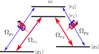
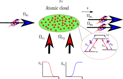
Figure 1: (a) Schematic diagram of the double-$\Lambda$ atomic system. (b) The schematic of possible arrangement of an experiment. Atoms (four-level double-$\Lambda$ coupling scheme shown in red circle) inside atomic cloud. A pair of resonant control fields $\Omega_{c_{1}}$ and $\Omega_{c_{2}}$(which can be spatially dependent) prepare atoms in a CPT state (see down bellow for spatial variation of control fields). A first vortex probe beam $\Omega_{p_{1}}$, perpendicular to the control beams, propagates inside the atomic cloud. The same vorticity of the first vortex beam $\Omega_{p_{1}}$ is transferred to the second generated probe field $\Omega_{p_{2}}$.

Let us consider the double-$\Lambda$ scheme, depicted in Fig. 1 (a). We are interested in the propagation of two laser pulses with the Rabi frequencies $\Omega_{p_{1}}$ and $\Omega_{p_{2}}$ in a quantum medium consisting of atoms characterized by the double-$\Lambda$ configuration of the atom-light coupling. The two atomic lower states $|g_{1}\rangle$ and $|g_{2}\rangle$ are coupled to two excited states $|e_{1}\rangle$ and $|e_{2}\rangle$ via four laser fields characterized by the slowly varying amplitudes $\Omega_{p_{1}}$, $\Omega_{p_{2}}$, $\Omega_{c_{1}}$ and $\Omega_{c_{2}}$.

Applying the rotating-wave approximation, the Hamiltonian for the double-$\Lambda$ atomic system reads

$$H=-\Omega_{p_{1}}|e_{2}\rangle\langle g_{1}|-\Omega_{p_{2}}|e_{2}\rangle\langle g_{2}|-\Omega_{c_{1}}|e_{1}\rangle\langle g_{1}|-\Omega_{c_{2}}|e_{1}\rangle\langle g_{2}|+H.c.\,.$$ (1)

The Maxwell–Bloch equations (MBE) governing the dynamics of the probe fields $\Omega_{p_{1}}$ and $\Omega_{p_{2}}$ and two atomic coherences $\rho_{e_{2}g_{1}}$ and $\rho_{e_{2}g_{2}}$ are given by

$$\frac{\partial}{\partial t}\left[\begin{array}[]{c}\rho_{e_{2}g_{1}}\\ \rho_{e_{2}g_{2}}\end{array}\right]=-(i\delta+\Gamma)\left[\begin{array}[]{c}\rho_{e_{2}g_{1}}\\ \rho_{e_{2}g_{2}}\end{array}\right]+i\left[\begin{array}[]{cc}\rho_{g_{1}g_{1}}-\rho_{e_{2}e_{2}}&\rho_{g_{2}g_{1}}\\ \rho_{g_{1}g_{2}}&\rho_{g_{2}g_{2}}-\rho_{e_{2}e_{2}}\end{array}\right]\left[\begin{array}[]{c}\Omega_{p_{1}}\\ \Omega_{p_{2}}\end{array}\right]-i\rho_{e_{2}e_{1}}\left[\begin{array}[]{c}\Omega_{c_{1}}\\ \Omega_{c_{2}}\end{array}\right],$$ (2)

and

$$\frac{\partial}{\partial z}\left[\begin{array}[]{c}\Omega_{p_{1}}\\ \Omega_{p_{2}}\end{array}\right]+c^{-1}\frac{\partial}{\partial t}\left[\begin{array}[]{c}\Omega_{p_{1}}\\ \Omega_{p_{2}}\end{array}\right]=i\frac{\alpha\Gamma}{2L}\left[\begin{array}[]{c}\rho_{e_{2}g_{1}}\\ \rho_{e_{2}g_{2}}\end{array}\right].$$ (3)

Equation (2) for the atomic coherences is modeled by means of the Liouville equation $\frac{\partial}{\partial t}\rho=-i[H,\rho]/\hbar+L_{\rho}$ with $L_{\rho}$ describing the decay of the system. On the other hand, Eq. (3) for the evolution of the probe fields is written under the slowly varying envelope approximation. In the latter equation $\alpha$ determines the optical density of the medium with a length $L$, and $\Gamma$ is the rate of spontaneous decay rate of the excited states. We have assumed the same single photon detuning for both probe fields in above equations, $\delta_{1}=\delta_{2}=\delta$, where $\delta_{1}=\omega_{p_{1}}-\omega_{e_{2}g_{1}}$ and $\delta_{2}=\omega_{p_{2}}-\omega_{e_{2}g_{2}}$, with $\omega_{p_{i}}$ being the central frequency of the corresponding probe fields. The control fields are taken to be in exact resonance with the corresponding atomic transitions.

The diffraction terms containing the transverse derivatives $(2k_{p_{1}})^{-1}\nabla_{\perp}^{2}\Omega_{p_{1}}$ and $(2k_{p_{2}})^{-1}\nabla_{\perp}^{2}\Omega_{p_{2}}$ have been disregarded in the Maxwell equation (3), where $k_{p_{1}}=\omega_{p_{1}}/c$ and $k_{p_{2}}=\omega_{p_{2}}/c$ represent the central wave vectors of the first and second probe beams. These terms can be evaluated as $\nabla_{\perp}^{2}\Omega_{p_{1(2)}}\sim w^{-2}\Omega_{p_{1(2)}}$, where $w$ is a characteristic transverse dimension of the laser beams. It can be a width of the vortex core if the beam carries an optical vortex or a characteristic width of the beam when there is no vortex. The change of the phase of the probe beams due to the diffraction term after passing the medium is then estimated to be $L/2kw^{2}$, where $L$ is the length of the atomic cloud, with $k\approx k_{p_{1(2)}}$. One can neglect the phase change $L/2kw^{2}$ when the sample length $L$ is not too large, $L\lambda/w^{2}\ll\pi$, where $\lambda=2\pi/k$ is an optical wavelength. For example, by taking the length of the atomic cloud to be $L=100\,\mathrm{\mu m}$, the characteristic transverse dimension of the beams $w=20\,\mathrm{\mu m}$ and the wavelength $\lambda=1\,\mathrm{\mu m}$, one obtains $L\lambda/w^{2}=0.25$. Under these conditions the diffraction terms do not play an important role and one can safely drop it out in Eq. (3).

Let us assume a situation where a pair of resonant strong control fields acting on the lower legs of the double-$\Lambda$ prepare the atoms in a CPT (or dark) state

$$|D\rangle=\cos\theta_{c}|g_{1}\rangle-\sin\theta_{c}|g_{2}\rangle,$$ (4)

where a mixing angle $\theta_{c}$ is defined by the equation

$$\left[\begin{array}[]{c}\cos\theta_{c}\\ \sin\theta_{c}\end{array}\right]=\frac{1}{\sqrt{|\Omega_{c_{1}}|^{2}+|\Omega_{c_{2}}|^{2}}}\left[\begin{array}[]{c}\Omega_{c_{2}}\\ \Omega_{c_{1}}\end{array}\right]\,.$$ (5)

Consequently, a weak probe pulse pair propagates in a coherently prepared medium interacting with the upper legs of double $\Lambda$ scheme.

Since the probe fields are much weaker than the control fields, $|\Omega_{p_{1}}|,|\Omega_{p_{2}}|\ll\sqrt{|\Omega_{c_{1}}|^{2}+|\Omega_{c_{2}}|^{2}}$, the atomic coherence $\rho_{g_{2}g_{1}}$ as well as the populations $\rho_{g_{1}g_{1}}$ and $\rho_{g_{2}g_{2}}$ change little during the propagation of the probe fields, giving

$$\left[\begin{array}[]{c}\rho_{g_{2}g_{1}}\\ \rho_{g_{1}g_{1}}\\ \rho_{g_{2}g_{2}}\end{array}\right]=\left[\begin{array}[]{c}-\sin\theta_{c}\cos\theta_{c}\\ \cos^{2}\theta_{c}\\ \sin^{2}\theta_{c}\end{array}\right]\,.$$ (6)

In addition, when $|\Omega_{p_{1}}|,|\Omega_{p_{2}}|\ll\Gamma$, the excited states are weakly populated, $\rho_{e_{2}g_{1}},\rho_{e_{2}g_{2}}\ll 1$, and Eq. (2) changes to

$$\frac{\partial}{\partial t}\left[\begin{array}[]{c}\rho_{e_{2}g_{1}}\\ \rho_{e_{2}g_{2}}\end{array}\right]=-(i\delta+\Gamma)\left[\begin{array}[]{c}\rho_{e_{2}g_{1}}\\ \rho_{e_{2}g_{2}}\end{array}\right]+i\left[\begin{array}[]{cc}\cos^{2}\theta_{c}&-\sin\theta_{c}\cos\theta_{c}\\ -\sin\theta_{c}\cos\theta_{c}&\sin^{2}\theta_{c}\end{array}\right]\left[\begin{array}[]{c}\Omega_{p_{1}}\\ \Omega_{p_{2}}\end{array}\right],$$ (7)

Then, to the first order, the following steady state solutions for the coherences $\rho_{e_{2}g_{1}}$, $\rho_{e_{2}g_{2}}$are obtained

$$(\delta-i\Gamma)\left[\begin{array}[]{c}\rho_{e_{2}g_{1}}\\ \rho_{e_{2}g_{2}}\end{array}\right]=\left[\begin{array}[]{cc}\cos^{2}\theta_{c}&-\sin\theta_{c}\cos\theta_{c}\\ -\sin\theta_{c}\cos\theta_{c}&\sin^{2}\theta_{c}\end{array}\right]\left[\begin{array}[]{c}\Omega_{p_{1}}\\ \Omega_{p_{2}}\end{array}\right]\,.$$ (8)

Substituting Eq. (8) into the Maxwell equations (3), one arrives at the following coupled equations for the propagation of the pulse pair

$$\frac{\partial}{\partial z}\left[\begin{array}[]{c}\Omega_{p_{1}}\\ \Omega_{p_{2}}\end{array}\right]=-iK\left[\begin{array}[]{c}\Omega_{p_{1}}\\ \Omega_{p_{2}}\end{array}\right],$$ (9)

with

$$K=\beta\left[\begin{array}[]{cc}\cos^{2}\theta_{c}&-\sin\theta_{c}\cos\theta_{c}\\ -\sin\theta_{c}\cos\theta_{c}&\sin^{2}\theta_{c}\end{array}\right],$$ (10)

and

$$\beta=\frac{\alpha\Gamma}{2L(i\Gamma-\delta)}.$$ (11)

From Eq. (9) follows that the probe field intensity will oscillate when the two-photon detuning $\delta$ is not zero (Shpaisman et al., 2004; Eilam et al., 2006). In addition, as can be seen from Eqs. (9) and (11), $\delta\neq 0$ introduces additional probe filed losses because $\beta$ acquires a real part. In the following, we consider the case when $\delta=0$ to minimize energy losses of the probe fields.

Let us assume that entrance to the medium the second probe field is absent $\Omega_{p_{2}}(0)=0$, while the first probe field $\Omega_{p_{1}}$ is a vortex beam defined by

$$\Omega_{p_{1}}(0)=\Omega(r)=\Omega_{p_{10}}\left(\frac{r}{w}\right)^{|l|}e^{-r^{2}/w^{2}}e^{il\phi},$$ (12)

where $l$ is the orbital angular momenta along the propagation axis $z$, and $\phi$ is the azimuthal angle, $r$ describes a cylindrical radius, $w$ is a beam waist, and $\Omega_{p_{10}}$ represents the strength of the vortex beam. The solutions to the Eq. (9) read

$$\left[\begin{array}[]{c}\Omega_{p_{1}}(z)\\ \Omega_{p_{2}}(z)\end{array}\right]=\Omega(r)\left[\begin{array}[]{c}\cos^{2}\theta_{c}e^{-i\beta z}+\sin^{2}\theta_{c}\\ -\sin\theta_{c}\cos\theta_{c}\left(e^{-i\beta z}-1\right)\end{array}\right].$$ (13)

Evidently, the laser beam $\Omega_{p_{1}}$ transfers its vortex to the generated beam $\Omega_{p_{2}}$. The intensity of both new probe field vortices can be manipulated by the Rabi-frequencies of control fields (see Eq. (6)).

At the beginning of the atomic cloud where the first probe vortex beam $\Omega_{p_{1}}(0)$ has just entered, the second probe beam is still absent ($\Omega_{p_{2}}(0)=0$), and it is generated going deeper into the atomic medium. As can be seen from Eq. (13), both vortex beams are not affected considerably by the losses during their propagation as long as the optical density length is large enough. In fact, the losses take place mostly at the entrance of the medium. If optical density of the resonant medium is sufficiently large $\alpha\gg 1$, the absorption length $L_{\mathrm{abs}}=L/\alpha$ constitutes a fraction of the whole medium $L_{\mathrm{abs}}\ll L$. For larger propagating distances $z\gg L_{\mathrm{abs}}$, the losses disappear

$$\left[\begin{array}[]{c}\Omega_{p_{1}}(z\gg L_{abs})\\ \Omega_{p_{2}}(z\gg L_{abs})\end{array}\right]=\Omega(r)\left[\begin{array}[]{c}\sin^{2}\theta_{c}\\ \sin\theta_{c}\cos\theta_{c}\end{array}\right],$$ (14)

and the system goes to the dark state given by Eq. (4) (see also Fig. 2).

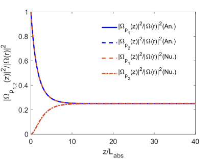
Figure 2: Analytical and numerical results of the dimensionless intensities of the light fields $|\Omega_{p_{1}}(z)|^{2}/|\Omega(r)|^{2}$ and $|\Omega_{p_{2}}(z)|^{2}/|\Omega(r)|^{2}$ against the dimensionless distance $z/L_{abs}$ for $\Omega_{c_{1}}=\Omega_{c_{2}}=\Gamma$, $\delta=0$ and $\alpha=40$. Analytical results are plotted based on Eq. (13), while numerical results are based on the full Optical-Bloch equations given by Eqs. (50)-(58) together with the Maxwell equation (3). For the numerical simulations, the incident form of probe pulse is $\Omega_{p_{1}}(z=0,t)=\Omega_{p_{1}}^{0}e^{-(t-t_{0})^{2}/2\bar{t}^{2}}$while $\Omega_{p_{2}}(z=0,t)=0$. The parameters used for the numerical calculations are $\Omega_{p_{1}}^{0}=0.01\Gamma$, $t_{0}=25$ and $\bar{t}=10$. Abbreviations "An." and "Nu." in plots stand for Analytical and Numerical results.

Let us consider the efficiency of frequency conversion from initial vortex beam $\Omega_{p_{1}}$ to the generated vortex beam $\Omega_{p_{2}}$ for $z\gg L_{\mathrm{abs}}$ described by Eq. (14). The efficiency of vortex conversion between different frequencies is

$$\eta=|\Omega_{p_{2}}(z\gg L_{abs})/\Omega_{p_{1}}(0)|=|\rho_{g_{1}g_{2}}|=\sin\theta_{c}\cos\theta_{c}.$$ (15)

Clearly, the maximum frequency conversion between vortex beams achieved in this way is only $1/2$ (when the coherence $\rho_{g_{1}g_{2}}$ is maximum). In the next section, we present another scenario for transfer of optical vortices in such a medium with the possibility to achieve the unit efficiency of the vortex conversion.

III Spatially dependent control fields

Let us consider a situation where two strong resonant control laser fields $\Omega_{c_{1}}(z)$ and $\Omega_{c_{2}}(z)$ are spatially dependent. This is the case if the control beams propagate perpendicular to the probe beams (Fig. 1 (b)), the latter beams propagating along the $z$ axis. In that case $\Omega_{c_{1}}(z)$ and $\Omega_{c_{2}}(z)$ represent the transverse profiles of the control beams. Application of such control fields prepare the system in the spatially dependent dark state $|D(z)\rangle$ immune to the spontaneously decay

$$|D(z)\rangle=\cos\theta(z)|g_{1}\rangle-\sin\theta(z)|g_{2}\rangle,$$ (16)

with

$$\left[\begin{array}[]{c}\cos\theta(z)\\ \sin\theta(z)\end{array}\right]=\frac{1}{\sqrt{|\Omega_{c_{1}}(z)|^{2}+|\Omega_{c_{2}}(z)|^{2}}}\left[\begin{array}[]{c}\Omega_{c_{2}}(z)\\ \Omega_{c_{1}}(z)\end{array}\right],$$ (17)

where $\theta(z)$ is the position-dependent mixing angle which differs from the constant mixing angle $\theta_{c}$ used in previous section. Again the interaction of probe fields with the medium is considered to be sufficiently weak, so it does not affect significantly the evolution of the density matrix, which is determined mostly by the coupling fields entering the density matrix equations. This means that one can use the results from a strongly driven $\Lambda$ system for the lower atomic states when the probe fields only act as a weak perturbation that does not change the density matrix elements

$$\left[\begin{array}[]{c}\rho_{g_{2}g_{1}}(z)\\ \rho_{g_{1}g_{1}}(z)\\ \rho_{g_{2}g_{2}}(z)\end{array}\right]=\left[\begin{array}[]{c}-\sin\theta(z)\cos\theta(z)\\ \cos^{2}\theta(z)\\ \sin^{2}\theta(z)\end{array}\right].$$ (18)

The approximate solutions to the density matrix equations read

$$(\delta-i\Gamma)\left[\begin{array}[]{c}\rho_{e_{2}g_{1}}(z)\\ \rho_{e_{2}g_{2}}(z)\end{array}\right]=\left[\begin{array}[]{cc}\cos^{2}\theta(z)&-\sin\theta(z)\cos\theta(z)\\ -\sin\theta(z)\cos\theta(z)&\sin^{2}\theta(z)\end{array}\right]\left[\begin{array}[]{c}\Omega_{p_{1}}(z)\\ \Omega_{p_{2}}(z)\end{array}\right],$$ (19)

and the propagation equations become

$$\frac{\partial}{\partial z}\left[\begin{array}[]{c}\Omega_{p_{1}}(z)\\ \Omega_{p_{2}}(z)\end{array}\right]=-iK(z)\left[\begin{array}[]{c}\Omega_{p_{1}}(z)\\ \Omega_{p_{2}}(z)\end{array}\right],$$ (20)

with

$$K(z)=\beta\left[\begin{array}[]{cc}\cos^{2}\theta(z)&-\sin\theta(z)\cos\theta(z)\\ -\sin\theta(z)\cos\theta(z)&\sin^{2}\theta(z)\end{array}\right].$$ (21)

There is no general analytical solution of the propagation equation (20) as the coefficients of the propagation matrix Eq. (21) are spatially dependent. Equation (20) is similar to a time-dependent Schrodinger equation with the time-dependence replaced with spatial dependence ($t\rightarrow z$). In this case, the propagation matrix $K(z)$ featured in Eq. (21) resembles a time-dependent Hamiltonian. When the Hamiltonian is time-dependent, general solutions are available if the dynamics satisfies adiabaticity (Bergmann et al., 1998; Paspalakis and Kis, 2002b). Therefore, we follow a standard adiabatic approximation method to study the evolution of the system. Yet the adiabatic evolution here refers to the spatial evolution. The eigenstates of the propagation matrix $K(z)$ in Eq. (21) can be written as

$$a^{0}= \left[\begin{array}[]{c}\sin\theta(z)\\ \cos\theta(z)\end{array}\right],$$ (24)

$$a^{\beta}= \left[\begin{array}[]{c}\cos\theta(z)\\ -\sin\theta(z)\end{array}\right],$$ (27)

where the two eigenstates $a^{0}$ and $a^{\beta}$ are orthogonal. It is straightforward to verify that the corresponding eigenenergies of the propagation matrix (21) are

$$\lambda^{0}= 0,$$ (28)

$$\lambda^{\beta}= \beta.$$ (29)

Let us form a unitary matrix $U$ as

$$U(z)=\left[\begin{array}[]{cc}\sin\theta(z)&\cos\theta(z)\\ \cos\theta(z)&-\sin\theta(z)\end{array}\right].$$ (30)

The matrix $U$ then transforms Eq. (20) to the adiabatic basis given by Eqs. (24)-(29)

$$\frac{\partial}{\partial z}\left[\begin{array}[]{c}\tilde{\Omega}_{p_{1}}(z)\\ \tilde{\Omega}_{p_{2}}(z)\end{array}\right]=-i\tilde{K}(z)\left[\begin{array}[]{c}\tilde{\Omega}_{p_{1}}(z)\\ \tilde{\Omega}_{p_{2}}(z)\end{array}\right],$$ (31)

where

$$\left[\begin{array}[]{c}\tilde{\Omega}_{p_{1}}(z)\\ \tilde{\Omega}_{p_{2}}(z)\end{array}\right]=U(z)^{-1}\left[\begin{array}[]{c}\Omega_{p_{1}}(z)\\ \Omega_{p_{2}}(z)\end{array}\right],$$ (32)

with the transformed propagation matrix $\tilde{K}(z)$ given by

$$\tilde{K}(z)=-iU(z)^{-1}\frac{\partial}{\partial z}U(z)+U(z)^{-1}K(z)U(z).$$ (33)

In the matrix form it reads

$$\tilde{K}(z)=i\left[\begin{array}[]{cc}0&\cos\theta(z)\frac{\partial}{\partial z}\sin\theta(z)-\sin\theta(z)\frac{\partial}{\partial z}\cos\theta(z)\\ -\cos\theta(z)\frac{\partial}{\partial z}\sin\theta(z)+\sin\theta(z)\frac{\partial}{\partial z}\cos\theta(z)&\beta\end{array}\right].$$ (34)

As can be seen, the eigenvalue $\beta$ appears in the diagonal of $\tilde{K}(z)$ which generally describes attenuation. However, for sufficiently long propagation distances, the field component along the eigenstate $a^{\beta}$ vanishes. The adiabaticity limit constrains that the off-diagonal elements of $\tilde{K}(z)$ are negligible compared to the difference of the diagonal ones

$$|\cos\theta(z)\frac{\partial}{\partial z}\sin\theta(z)-\sin\theta(z)\frac{\partial}{\partial z}\cos\theta(z)|\ll|\beta|.$$ (35)

When the adiabaticity condition (35) is fulfilled, the solution of the propagation equation (20) reads

$$\left[\begin{array}[]{c}\Omega_{p_{1}}(z)\\ \Omega_{p_{2}}(z)\end{array}\right]=U(z)WU(z)^{-1}\left[\begin{array}[]{c}\Omega_{p_{1}}(z_{i})\\ \Omega_{p_{2}}(z_{i})\end{array}\right],$$ (36)

where

$$W=\left[\begin{array}[]{cc}e^{-i\int_{z_{i}}^{z}\tilde{K}_{11}(z)dz}&0\\ 0&e^{-i\int_{z_{i}}^{z}\tilde{K}_{22}(z)dz}\end{array}\right].$$ (37)

For a long propagation distance $(z\gg L_{abs})$, the exponential term $e^{-i\int_{z_{i}}^{z}\tilde{K}_{22}(z)dz}$ vanishes. In this limit the solutions to the Eq. (36) read

$$\left[\begin{array}[]{c}\Omega_{p_{1}}(z)\\ \Omega_{p_{2}}(z)\end{array}\right]=\Omega(r)\left[\begin{array}[]{c}\sin\theta(z_{i})\sin\theta(z)\\ \sin\theta(z_{i})\cos\theta(z)\end{array}\right],$$ (38)

where we have assumed that at the entry of the medium $\Omega_{p_{1}}(z_{i})$ is a vortex ($\Omega_{p_{1}}(z_{i})=\Omega(r)$) and $\Omega_{p_{2}}(z_{i})=0$. As one can see from Eq. (38), in this case the same vorticity of the first vortex beam $\Omega_{p_{1}}(z_{i})$ is transferred to the second generated field $\Omega_{p_{2}}(z)$.

Let us consider a situation where at the beginning of the medium the first control field is present ($|\Omega_{c_{1}}(z_{i})|=1$) while the second control field is zero ($|\Omega_{c_{2}}(z_{i})|=0$), giving

$$\left[\begin{array}[]{c}|\sin\theta(z_{i})|\\ |\cos\theta(z_{i})|\end{array}\right]=\left[\begin{array}[]{c}1\\ 0\end{array}\right].$$ (39)

Moreover, we assume that the first control field is zero at the end of the medium $|\Omega_{c_{1}}(z_{f})|=0$ while we have $|\Omega_{c_{2}}(z_{f})|=1$, resulting

$$\left[\begin{array}[]{c}|\sin\theta(z_{f})|\\ |\cos\theta(z_{f})|\end{array}\right]=\left[\begin{array}[]{c}0\\ 1\end{array}\right],$$ (40)

In that case the efficiency of vortex conversion between different frequencies is obtained to be the unity using Eqs. (38)-(40):

$$\eta=|\Omega_{p_{2}}(z_{f})/\Omega(r)|=1,$$ (41)

This is illustrated in Fig. 3 showing the dependence of the intensities $|\Omega_{p_{1}}(z)|^{2}/|\Omega(r)|^{2}$ and $|\Omega_{p_{2}}(z)|^{2}/|\Omega(r)|^{2}$ given by Eq. (38) on the dimensionless distance $z/L_{abs}$ for the resonance case $\delta=0$ and for the optical depth $\alpha=40$.

The amplitudes of the spatially dependent control fields satisfying Eqs. (39)-(40) can be chosen as

$$\left[\begin{array}[]{c}\Omega_{c_{1}}(z)\\ \Omega_{c_{2}}(z)\end{array}\right]=\Omega_{c}\left[\begin{array}[]{c}\sqrt{\frac{1}{1+e^{(z-z_{0})/\bar{z}}}}\\ \sqrt{\frac{1}{1+e^{-(z-z_{0})/\bar{z}}}}\end{array}\right],$$ (42)

where $\Omega_{c_{1}}^{2}(z)+\Omega_{c_{1}}^{2}(z)=\Omega_{c}^{2}$ (see Fig. 3(a)). Figure 3(b) illustrates that although initially at the beginning of the atomic medium the first probe field $\Omega_{p_{1}}(z)$ exists, going deeper through the medium it disappears while the second probe field $\Omega_{p_{2}}(z)$ is generated.

Note that although Eq. (38) does not show to have any limitations, we have used the adiabatic approximation to obtain it. This approximation is not valid when the light fields change too fast in space (or in time). Hence, one needs to find an optimal condition, when the adiabatic approximation is valid. Inserting the spatially dependent control fields given by Eq. (42) into the adiabatic condition (35) one gets for the resonant case $\delta=0$:

$$|\frac{1}{\bar{z}}\sqrt{\frac{1}{2+2\cosh\left((z-z_{0})/\bar{z}\right)}}|\ll|\frac{1}{L_{\mathrm{abs}}}|.$$ (43)

At the position where the left hand side of Eq. (43) is the largest ($z=z_{0}$), the condition (43) requires that

$$\bar{z}\gg L_{\mathrm{abs}}\,.$$ (44)

To satisfy the adiabaticity requirement given by Eq. (44), we can take, for example $\bar{z}=2L_{abs}$. The position $z_{0}$ should be in the middle of the atomic medium $z_{0}=\alpha L_{\mathrm{abs}}/2$. Furthermore to satisfy Eqs. (39)–(40), the length of the medium should be much larger than $\bar{z}$. Thus we can take $z_{0}=20L_{\mathrm{abs}}$ and thus the total length $40L_{\mathrm{abs}}$.

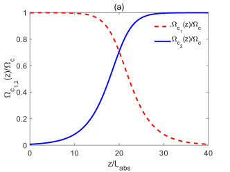
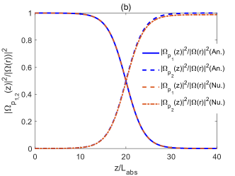
Figure 3: (a) Dependence of the dimensionless spatially dependent control fields given in Eq. (42). (b) Analytical and numerical results of the dimensionless intensities of the light fields $|\Omega_{p_{1}}(z)|^{2}/|\Omega(r)|^{2}$ and $|\Omega_{p_{2}}(z)|^{2}/|\Omega(r)|^{2}$ against the dimensionless distance $z/L_{abs}$ and for $\bar{z}=2L_{abs}$, $z_{0}=20L_{abs}$, $\alpha=40$ and $\delta=0$. Analytical results are plotted based on Eq. (38), while numerical results are based on the full Optical-Bloch equations given by Eqs. (50)-(58) together with the Maxwell equation (3). For the numerical simulations, the incident form of probe pulses are the same as Fig. 2. Abbreviations "An." and "Nu." in plots stand for Analytical and Numerical results.

Next we work with the spatially dependent Gaussian-shaped control fields (Fig. 4(a)) centered on $z=0$ and $z=L$ and satisfying Eqs. (39)–(40)

$$\left[\begin{array}[]{c}\Omega_{c_{1}}(z)\\ \Omega_{c_{2}}(z)\end{array}\right]=\Omega_{c}\left[\begin{array}[]{c}e^{-z^{2}/\sigma^{2}}\\ e^{-(z-L)^{2}/\sigma^{2}}\end{array}\right],$$ (45)

which is experimentally more feasible to produce. Substituting the Gaussian-shaped control fields given by Eq. (45) into the adiabatic condition (35) results in ($\delta=0$):

$$|\frac{2Le^{L(L+2z)/\sigma^{2}}}{\sigma^{2}\left(e^{2L^{2}/\sigma^{2}}+e^{4Lz/\sigma^{2}}\right)}|\ll|\frac{1}{L_{\mathrm{abs}}}|.$$ (46)

At the position $z=L/2$ where the left hand side of Eq. (46) has a maximum, one gets

$$\sigma\gg L\sqrt{\frac{1}{\alpha}}.$$ (47)

On the other hand, we want to have intensity on one side of the medium large, on another side almost zero. This requires

$$\sigma\ll L.$$ (48)

The requirements Eq. (47) and (48) together lead to

$$\alpha\gg 1.$$ (49)

As can be seen from 4(b), the first probe field $\Omega_{p_{1}}(z)$ vanishes during propagating through the medium and the second probe field $\Omega_{p_{2}}(z)$ is generated. For the simulations we select $\alpha=40$ and $\sigma=16$ satisfying Eqs. (47)-(49).

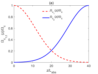
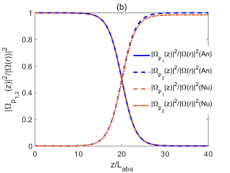
Figure 4: (a) Dependence of the dimensionless spatially dependent control fields given in Eq. (45). (b) Analytical and numerical results of the dimensionless intensities of the light fields $|\Omega_{p_{1}}(z)|^{2}/|\Omega(r)|^{2}$ and $|\Omega_{p_{2}}(z)|^{2}/|\Omega(r)|^{2}$ against the dimensionless distance $z/L_{abs}$ and for $\alpha=40$, $\sigma=16$ and $\delta=0$. Analytical results are plotted based on Eq. (38), while numerical results are based on the full Optical-Bloch equations given by Eqs. (50)-(58) together with the Maxwell equation (3). For the numerical simulations, the incident form of probe pulses are the same as Fig. 2. Abbreviations "An." and "Nu." in plots stand for Analytical and Numerical results.

The validity of our adiabatic method is tested by the numerical results based on the full Maxwell-Bloch equations given by Eqs. (50)-(58) and (3), and a very good agreement is observed, see Figs. 3 and 4.

IV Concluding Remarks

In summary, we have considered propagation of optical vortices in a cloud of cold atoms characterized by the double-$\Lambda$ configuration of the atom-light coupling and derived an approximate adiabatic equation (38) describing such a propagation. The equation shows that when the adiabaticity condition (35) is satisfied, the OAM can be exchanged between probe pulse pair with a maximum efficiency of $100\%$. It has been recently shown that a double-$\Lambda$ scheme can be employed for the exchange of optical vortices based on the EIT (Hamedi et al., 2018a). Moreover, the transfer of optical vortices in coherently prepared $n+1$-level structures has been also demonstrated (Hamedi et al., 2019). However, a complete energy conversion between optical vortices is not possible in both previous studies.

The current approach for the exchange and complete conversion of optical vortices resembles the STIRAP. Yet in our proposal the roles of the atomic states and the light fields are interchanged. It is the atomic states in the STIRAP which are transferred by properly choosing the time dependence of the light fields. In contrast, in the present situation the energy is transferred between the light beams by properly choosing the position dependence of the atomic states.

The proposed double-$\Lambda$ setup can be implemented experimentally for example using the ${}^{87}Rb$ atoms. To have a well-defined polarization, the control beam propagating orthogonal to the probe should be linearly polarized along the probe beam direction. The lower levels $|g_{1}\rangle$ and $|g_{2}\rangle$ can then correspond to the $|5S_{1/2},F=1,m_{F}=1\rangle$ $|5S_{1/2},F=2,m_{F}=2\rangle$ hyperfine states. The excited states $|e_{1}\rangle$ and $|e_{2}\rangle$ can be $|e_{1}\rangle=|5P_{1/2},F=2,m_{F}=2\rangle$ and $|e_{2}\rangle=|5P_{3/2},F=2,m_{F}=2\rangle$, respectively. The excited state decay rate $\Gamma$ is $\sim 2\pi\times 6\,MHz$ for ${}^{87}Rb$ atoms. We have assumed an optical depth of $40$ which is experimentally feasible (Chiu et al., 2014; Hsiao et al., 2014). Rabi frequencies of the control beams are of the order of $\Gamma$. In the present study the Rabi frequencies of the probe fields should be much smaller than the Rabi frequencies of the control beams.

Appendix A Full Optical-Bloch equations

To make the numerical calculations, we solve the following equations that describe the time evolution of density matrix operator of the atoms together with the Maxwell equations for the propagation of probe fields:

$$\dot{\rho}_{e_{2}g_{1}} =i\Omega_{p_{1}}\rho_{g_{1}g_{1}}+i\Omega_{p_{2}}\rho_{g_{2}g_{1}}-i\Omega_{c_{1}}\rho_{e_{2}e_{1}}-i\Omega_{p_{1}}\rho_{e_{2}e_{2}}-(\Gamma_{e_{2}g_{1}}+i\Delta_{e_{2}g_{1}})\rho_{e_{2}g_{1}},$$ (50)

$$\dot{\rho}_{e_{2}g_{2}} =i\Omega_{p_{2}}\rho_{g_{2}g_{2}}+i\Omega_{p_{1}}\rho_{g_{1}g_{2}}-i\Omega_{c_{2}}\rho_{e_{2}e_{1}}-i\Omega_{p_{2}}\rho_{e_{2}e_{2}}-(\Gamma_{e_{2}g_{2}}+i\Delta_{e_{2}g_{2}})\rho_{e_{2}g_{2}},$$ (51)

$$\dot{\rho}_{e_{2}e_{1}} =i\Omega_{p_{1}}\rho_{g_{1}e_{1}}+i\Omega_{p_{2}}\rho_{g_{2}e_{1}}-i\Omega_{c_{1}}\rho_{e_{2}g_{1}}-i\Omega_{c_{2}}\rho_{e_{2}g_{2}}-(\Gamma_{e_{2}e_{1}}+i\Delta_{e_{2}e_{1}})\rho_{e_{2}e_{1}},$$ (52)

$$\dot{\rho}_{e_{1}g_{1}} =i\Omega_{c_{1}}\rho_{g_{1}g_{1}}+i\Omega_{c_{2}}\rho_{g_{2}g_{1}}-i\Omega_{c_{1}}\rho_{e_{1}e_{1}}-i\Omega_{p_{1}}\rho_{e_{1}e_{2}}-(\Gamma_{e_{1}g_{1}}+i\Delta_{e_{1}g_{1}})\rho_{e_{1}g_{1}},$$ (53)

$$\dot{\rho}_{e_{1}g_{2}} =i\Omega_{c_{2}}\rho_{g_{2}g_{2}}+i\Omega_{c_{1}}\rho_{g_{1}g_{2}}-i\Omega_{c_{2}}\rho_{e_{1}e_{1}}-i\Omega_{p_{2}}\rho_{e_{1}e_{2}}-(\Gamma_{e_{1}g_{2}}+i\Delta_{e_{1}g_{2}})\rho_{e_{1}g_{2}},$$ (54)

$$\dot{\rho}_{g_{2}g_{1}} =i\Omega_{c_{2}}\rho_{e_{1}g_{1}}+i\Omega_{p_{2}}\rho_{e_{2}g_{1}}-i\Omega_{c_{1}}\rho_{g_{2}e_{1}}-i\Omega_{p_{1}}\rho_{g_{2}e_{2}}-(\Gamma_{g_{2}g_{1}}+i\Delta_{g_{2}g_{1}})\rho_{g_{2}g_{1}},$$ (55)

$$\dot{\rho}_{g_{1}g_{1}} =i\Omega_{c_{1}}(\rho_{e_{1}g_{1}}-\rho_{g_{1}e_{1}})+i\Omega_{p_{1}}(\rho_{e_{2}g_{1}}-\rho_{g_{1}e_{2}})+\gamma_{e_{1}g_{1}}\rho_{e_{1}e_{1}}+\gamma_{e_{2}g_{1}}\rho_{e_{2}e_{2}},$$ (56)

$$\dot{\rho}_{g_{2}g_{2}} =i\Omega_{c_{2}}(\rho_{e_{1}g_{2}}-\rho_{g_{2}e_{1}})+i\Omega_{p_{2}}(\rho_{e_{2}g_{2}}-\rho_{g_{2}e_{2}})+\gamma_{e_{1}g_{2}}\rho_{e_{1}e_{1}}+\gamma_{e_{2}g_{2}}\rho_{e_{2}e_{2}},$$ (57)

$$\dot{\rho}_{e_{2}e_{2}} =i\Omega_{p_{1}}(\rho_{g_{1}e_{2}}-\rho_{e_{2}g_{1}})+i\Omega_{p_{2}}(\rho_{g_{2}e_{2}}-\rho_{e_{2}g_{2}})-(\gamma_{e_{2}g_{1}}+\gamma_{e_{2}g_{2}})\rho_{e_{2}e_{2}},$$ (58)

where $\rho_{g_{1}g_{1}}+\rho_{g_{2}g_{2}}+\rho_{e_{1}e_{1}}+\rho_{e_{2}e_{2}}=1$. In numerical simulations we take $\gamma_{e_{1}g_{1}}=\gamma_{e_{2}g_{2}}=\gamma_{e_{1}g_{2}}=\gamma_{e_{2}g_{1}}=\Gamma$, $\Gamma_{e_{2}g_{1}}=\Gamma_{e_{2}g_{2}}=\Gamma_{e_{1}g_{1}}=\Gamma_{e_{1}g_{2}}=\Gamma$, $\Gamma_{g_{1}g_{2}}=0$, $\Gamma_{e_{2}e_{1}}=2\Gamma$, $\Delta_{e_{2}g_{1}}=\Delta_{e_{2}g_{2}}=\delta$ and $\Delta_{e_{2}e_{1}}=\Delta_{e_{1}g_{1}}=\Delta_{e_{1}g_{2}}=\Delta_{g_{2}g_{1}}=0$.

References

- Alzetta et al. (1976) G. Alzetta, A. Gozzini, L. Moi, and G. Orriols, Nuovo Cimento B 36, 5 (1976).
- Gray et al. (1978) H. R. Gray, R. M. Whitley, and C. R. Stroud, Opt. Lett. 3, 218 (1978).
- Radmore and Knight (1982) P. M. Radmore and P. L. Knight, J. Phys. B: At. Mol. Phys. 15, 561 (1982).
- Hioe and Carroll (1988) F. T. Hioe and C. E. Carroll, Phys. Rev. A 37, 3000 (1988).
- Arimondo (1996) E. Arimondo, Progress in Optics 35, 257 (1996).
- Harris (1997) S. E. Harris, Physics Today 50, 36 (1997).
- Lukin (2003) M. D. Lukin, Rev. Mod. Phys. 75, 457 (2003).
- Fleischhauer et al. (2005) M. Fleischhauer, A. Imamoglu, and J. P. Marangos, Rev. Mod. Phys. 77, 633 (2005).
- Paspalakis and Knight (2002) E. Paspalakis and P. L. Knight, Phys. Rev. A 66, 015802 (2002).
- Kuklinski et al. (1989) J. R. Kuklinski, U. Gaubatz, F. T. Hioe, and K. Bergmann, Phys. Rev. A 40, 6741 (1989).
- Bergmann et al. (1998) K. Bergmann, H. Theuer, and B. W. Shore, Rev. Mod. Phys. 70, 1003 (1998).
- Ivanov et al. (2004) P. A. Ivanov, N. V. Vitanov, and K. Bergmann, Phys. Rev. A 70, 063409 (2004).
- Kumar et al. (2016) K. S. Kumar, A. Vepsalainen, S. Danilin, and G. S. Paraoanu, Nature Communications 7, 10628 (2016).
- Vepsalainen et al. (2019) A. Vepsalainen, S. Danilin, and G. S. Paraoanu, Science Advances 5, aau5999 (2019).
- Harris et al. (1990) S. E. Harris, J. E. Field, and A. Imamoğlu, Phys. Rev. Lett. 64, 1107 (1990).
- Deng et al. (1998) L. Deng, M. G. Payne, and W. R. Garrett, Phys. Rev. A 58, 707 (1998).
- Wang et al. (2001) H. Wang, D. Goorskey, and M. Xiao, Phys. Rev. Lett. 87, 073601 (2001).
- Kang and Zhu (2003) H. Kang and Y. Zhu, Phys. Rev. Lett. 91, 093601 (2003).
- Juzeliūnas and Öhberg (2004) G. Juzeliūnas and P. Öhberg, Phys. Rev. Lett. 93, 033602 (2004).
- Ruseckas et al. (2011a) J. Ruseckas, V. Kudriašov, G. Juzeliūnas, R. G. Unanyan, J. Otterbach, and M. Fleischhauer, Phys. Rev. A 83, 063811 (2011a).
- Braje et al. (2003) D. A. Braje, V. Balić, G. Y. Yin, and S. E. Harris, Phys. Rev. A 68, 041801 (2003).
- Zibrov et al. (2002) A. S. Zibrov, A. B. Matsko, O. Kocharovskaya, Y. V. Rostovtsev, G. R. Welch, and M. O. Scully, Phys. Rev. Lett. 88, 103601 (2002).
- Allen et al. (1999) L. Allen, M. J. Padgett, and M. Babiker, Progress in Optics 39, 291 (1999).
- Padgett et al. (2004) M. Padgett, J. Courtial, and L. Allen, Physics Today 57, 35 (2004).
- Allen et al. (1992) L. Allen, M. W. Beijersbergen, R. J. C. Spreeuw, and J. P. Woerdman, Phys. Rev. A 45, 8185 (1992).
- Babiker et al. (2019) M. Babiker, D. L. Andrews, and V. Lembessis, Journal of Optics 21, 013001 (2019).
- Babiker et al. (1994) M. Babiker, W. L. Power, and L. Allen, Phys. Rev. Lett. 73, 1239 (1994).
- Lembessis and Babiker (2010) V. E. Lembessis and M. Babiker, Phys. Rev. A 82, 051402 (2010).
- Lembessis et al. (2014) V. E. Lembessis, D. Ellinas, M. Babiker, and O. Al-Dossary, Phys. Rev. A 89, 053616 (2014).
- Chen et al. (2008) Q.-F. Chen, B.-S. Shi, Y.-S. Zhang, and G.-C. Guo, Phys. Rev. A 78, 053810 (2008).
- Ding et al. (2012) D.-S. Ding, Z.-Y. Zhou, B.-S. Shi, X.-B. Zou, and G.-C. Guo, Opt. Lett. 37, 3270 (2012).
- Walker et al. (2012) G. Walker, A. S. Arnold, and S. Franke-Arnold, Phys. Rev. Lett. 108, 243601 (2012).
- Radwell et al. (2015) N. Radwell, T. W. Clark, B. Piccirillo, S. M. Barnett, and S. Franke-Arnold, Phys. Rev. Lett. 114, 123603 (2015).
- Sharma and Dey (2017) S. Sharma and T. N. Dey, Phys. Rev. A 96, 033811 (2017).
- Hamedi et al. (2018a) H. R. Hamedi, J. Ruseckas, and G. Juzeliūnas, Phys. Rev. A 98, 013840 (2018a).
- Hamedi et al. (2018b) H. R. Hamedi, V. Kudriašov, J. Ruseckas, and G. Juzeliūnas, Optics Express 26, 28249 (2018b).
- Ruseckas et al. (2007) J. Ruseckas, G. Juzeliūnas, P. Öhberg, and S. M. Barnett, Phys. Rev. A 76, 053822 (2007).
- Ruseckas et al. (2011b) J. Ruseckas, A. Mekys, and G. Juzeliūnas, Phys. Rev. A 83, 023812 (2011b).
- Ruseckas et al. (2013) J. Ruseckas, V. Kudriašov, I. A. Yu, and G. Juzeliūnas, Phys. Rev. A 87, 053840 (2013).
- Dutton and Ruostekoski (2004) Z. Dutton and J. Ruostekoski, Phys. Rev. Lett. 93, 193602 (2004).
- Hamedi et al. (2019) H. R. Hamedi, J. Ruseckas, E. Paspalakis, and G. Juzeliūnas, Phys. Rev. A 99, 033812 (2019).
- Ruseckas et al. (2011c) J. Ruseckas, A. Mekys, and G. Juzeliūnas, J. Opt. 13, 064013 (2011c).
- Bortman-Arbiv et al. (2001) D. Bortman-Arbiv, A. D. Wilson-Gordon, and H. Friedmann, Phys. Rev. A 63, 031801 (2001).
- Wang et al. (2008) T. Wang, L. Zhao, L. Jiang, and S. F. Yelin, Phys. Rev. A 77, 043815 (2008).
- Pugatch et al. (2007) R. Pugatch, M. Shuker, O. Firstenberg, A. Ron, and N. Davidson, Phys. Rev. Lett. 98, 203601 (2007).
- Moretti et al. (2009) D. Moretti, D. Felinto, and J. W. R. Tabosa, Phys. Rev. A 79, 023825 (2009).
- Eberly et al. (1996) J. H. Eberly, A. Rahman, and R. Grobe, Phys. Rev. Lett. 76, 3687 (1996).
- Scully (1985) M. O. Scully, Phys. Rev. Lett. 55, 2802 (1985).
- Fleischhauer et al. (1992) M. Fleischhauer, C. H. Keitel, M. O. Scully, C. Su, B. T. Ulrich, and S.-Y. Zhu, Phys. Rev. A 46, 1468 (1992).
- Paspalakis et al. (2002) E. Paspalakis, N. J. Kylstra, and P. L. Knight, Phys. Rev. A 65, 053808 (2002).
- Paspalakis and Kis (2002a) E. Paspalakis and Z. Kis, Phys. Rev. A 66, 025802 (2002a).
- Paspalakis and Kis (2002b) E. Paspalakis and Z. Kis, Opt. Lett. 27, 1836 (2002b).
- Kis and Paspalakis (2003) Z. Kis and E. Paspalakis, Phys. Rev. A 68, 043817 (2003).
- Deng et al. (2005) L. Deng, M. G. Payne, G. Huang, and E. W. Hagley, Phys. Rev. E 72, 055601 (2005).
- Kang et al. (2011) H. Kang, B. Kim, Y. H. Park, C.-H. Oh, and I. W. Lee, Opt. Express 19, 4113 (2011).
- Eilam et al. (2006) A. Eilam, A. D. Wilson-Gordon, and H. Friedmann, Phys. Rev. A 73, 053805 (2006).
- Chiu et al. (2014) C.-K. Chiu, Y.-H. Chen, Y.-C. Chen, I. A. Yu, Y.-C. Chen, and Y.-F. Chen, Phys. Rev. A 89, 023839 (2014).
- Turnbull et al. (2013) M. T. Turnbull, P. G. Petrov, C. S. Embrey, A. M. Marino, and V. Boyer, Phys. Rev. A 88, 033845 (2013).
- Shpaisman et al. (2005) H. Shpaisman, A. D. Wilson-Gordon, and H. Friedmann, Phys. Rev. A 71, 043812 (2005).
- Chong and Soljačić (2008) Y. D. Chong and M. Soljačić, Phys. Rev. A 77, 013823 (2008).
- Moiseev and Ham (2006) S. A. Moiseev and B. S. Ham, Phys. Rev. A 73, 033812 (2006).
- Xu et al. (2013) X. Xu, S. Shen, and Y. Xiao, Opt. Express 21, 11705 (2013).
- Kang et al. (2006) H. Kang, G. Hernandez, J. Zhang, and Y. Zhu, Phys. Rev. A 73, 011802 (2006).
- Raczyński et al. (2004) A. Raczyński, J. Zaremba, and S. Zieli ńska Kaniasty, Phys. Rev. A 69, 043801 (2004).
- Liu et al. (2016) Z.-Y. Liu, Y.-H. Chen, Y.-C. Chen, H.-Y. Lo, P.-J. Tsai, I. A. Yu, Y.-C. Chen, and Y.-F. Chen, Phys. Rev. Lett. 117, 203601 (2016).
- Liu et al. (2004) X.-J. Liu, H. Jing, X.-T. Zhou, and M.-L. Ge, Phys. Rev. A 70, 015603 (2004).
- Korsunsky and Kosachiov (1999) E. A. Korsunsky and D. V. Kosachiov, Phys. Rev. A 60, 4996 (1999).
- Lee et al. (2016) C.-Y. Lee, B.-H. Wu, G. Wang, Y.-F. Chen, Y.-C. Chen, and I. A. Yu, Opt. Express 24, 1008 (2016).
- Juo et al. (2018) J.-Y. Juo, J.-K. Lin, C.-Y. Cheng, Z.-Y. Liu, I. A. Yu, and Y.-F. Chen, Phys. Rev. A 97, 053815 (2018).
- Shpaisman et al. (2004) H. Shpaisman, A. D. Wilson-Gordon, and H. Friedmann, Phys. Rev. A 70, 063814 (2004).
- Hsiao et al. (2014) Y.-F. Hsiao, H.-S. Chen, P.-J. Tsai, and Y.-C. Chen, Phys. Rev. A 90, 055401 (2014).