Bending models of lipid bilayer membranes:
spontaneous curvature and area-difference elasticity

Abstract

We preset a computational study of bending models for the curvature elasticity of lipid bilayer membranes that are relevant for simulations of vesicles and red blood cells. We compute bending energy and forces on triangulated meshes and evaluate and extend four well established schemes for their approximation: Kantor and Nelson [1], Jülicher [2], Gompper and Kroll [3] and Meyer et. al. [4], termed A, B, C, D. We present a comparative study of these four schemes on the minimal bending model and propose extensions for schemes B, C and D. These extensions incorporate the reference state and non-local energy to account for the spontaneous curvature, bilayer coupling, and area-difference elasticity models. Our results indicate that the proposed extensions enhance the models to account for shape transformation including budding/vesiculation as well as for non-axisymmetric shapes. We find that the extended scheme B is superior to the rest in terms of accuracy, and robustness as well as simplicity of implementation. We demonstrate the capabilities of this scheme on several benchmark problems including the budding-vesiculating process and the reproduction of the phase diagram of vesicles.

1 Introduction

Lipid bilayers are fundamental structural elements in biology. Vesicles are compartments enclosed by lipid bilayer membranes and they have been studied extensively over the last four decades [5, 6, 7, 8]. Notably vesicles have been the subject of investigations that were awarded the 2013 Nobel prize in the physiology or medicine (James Rothman, Randy Schekman and Thomas Südhof). A vesicle has a relatively simple structure when compared to other entities at cellular level and they have been the subject of several detailed theoretical [9, 10, 11, 12, 13, 14, 15, 16] and experimental studies [17, 18]. Models of vesicles are readily transferable to more complex structures, as lipid bilayer membranes enclose most cells and their nuclei as well as many viruses. Importantly, a lipid bilayer and a spectrin network constitute a red blood cell (RBC) membrane [19, 20].

Lipid membranes are a few nanometers thin, but they span surfaces that are in the order of micrometers. The bending elasticity of the quasi two-dimensional structures is caused by relative extension/compression of outer/inner surface, which can be expressed as a function of the membrane curvature [6, 7, 8]. Canham proposed the first form of membrane bending energy, that depends quadratically on the two principal curvatures of the surface [9]. This representation, along with constraints on total area and volume, constitutes the minimal model for a vesicle. Helfrich formulated a bending energy that includes a Gaussian curvature as well as a ”spontaneous” curvature $2H_{0}$ [10] that is attributed to chemical differences in two lipid layers. This is the spontaneous curvature (SC) model and by setting $H_{0}=0$, it is equivalent to the minimal model. In turn, Sheetz & Singer [11] and Evans [12] accounted for the density difference of the two lipid layers. Their work led to the bilayer couple (BC) model [13] that introduces a constraint on the area difference so that $\Delta A=\Delta A_{0}$, where $\Delta A$ and $\Delta A_{0}$ are the instantaneous and targeted area differences between the two lipid layers. A few years later three groups ([14, 15, 16]) proposed that the non-local bending energy has a quadratic form $(\Delta A-\Delta A_{0})^{2}$. Here $\Delta A_{0}$ reflects reference of the area difference between the two layers. This is area-difference elasticity (ADE) model, which degenerates to the minimal, SC or BC model as a special case. The ADE model has been validated experimentally on vesicles [21, 22].

Despite the well established formulation of these membrane models, simulations of vesicles and red-blood cells remain a challenging task. The key difficulty lies in the evaluation of the resulting forces. The bending force depends on the Laplace-Beltrami operator $\nabla^{2}_{s}$ on the mean curvature, which further relates to $\nabla^{2}_{s}$ of the coordinates on a surface. Hence, the evaluation of the bending force requires approximations of the fourth derivatives of the surface coordinates. A recent review showcased how computation of the bending energy and especially the force remain elusive, even for the minimal model [23]. These computations have similar difficulties as those met when calculating Willmore flow in differential geometry [7, 23], which are of particular interest to the computer graphics community [24].

One approach has focused on axi-symmetric shapes that reduces the calculations to solving Ordinary Differential Equations (ODEs) [5, 25, 26, 8]. Recent works have employed either spherical harmonic expansions/quadratic approximation to represent the surface [27, 28, 29, 30] or phase field [31] models. We note in particular level set methods for the description of the membrane surface [32, 33, 34] thus allowing for volume based calculations of the membrane dynamics and large deformations even with topological changes.

In this work, we represent the surface as a triangulated mesh, which has been used extensively to model vesicle and RBC membranes and they have been coupled to fluid solvers [35, 36, 37, 38, 39, 40]. However, the majority of vesicle and RBC simulations have employed only the minimal model. Exceptions are Monte Carlo simulations from groups of Seifert [41] and Wortis [42] and the finite element method from Barrett et al [43]. We examine and extend four established schemes for the discretization of the general bending model on a triangulated mesh [1, 2, 3, 4]. We perform a number of benchmark problems to compare their accuracy, robustness and stability.

The paper is structured as follows: we describe energy functionals of the minimal, SC, BC and ADE models in Section 2 and present an expression for the force density. In Section 3, we present the four discretization schemes (A, B, C, D) which have been previously applied to the minimal model [1, 2, 3, 4]. We extend schemes B, C, D to incorporate the spontaneous curvature and non-local bending energy thus accessing the SC, and BC/ADE models. The details of the derivations on Sections 2 and 3 can be found in A–G. In Section 4.1, we evaluate the proposed schemes on shapes with known analytical expressions for the energy and force. In Section 4.2 we compute the phase diagrams for oblate-stomatocyte, oblate-discocyte, prolate-dumbbell, prolate-cigar shapes described by the minimal model with the four discretization schemes, from different initial shapes such as prolate, oblate and sphere. Thereafter, we generate slices of phase diagrams of SC, BC and ADE models. We compare our results with solutions obtained by axi-symmetric ODEs, spherical harmonic as well as results from the program ”Surface Evolver” and experiments. In Section 4.4 we present results from dynamic simulations. We summarize our findings in Section 5.

2 Continuous energy and force

2.1 Energy functionals

The primary model for the two-dimensional membrane elasticity is based on an extension of one dimensional beam theory by Canham [9] with an energy functional:

$$E^{C}=\frac{\kappa_{b}}{2}\int(C^{2}_{1}+C^{2}_{2})dA,$$ (1)

where $\kappa_{b}$ is the bending elastic constant, $C_{1}$ and $C_{2}$ are the two principal curvatures and the integral is taken over a two-dimensional parametric surface embedded in three-dimensional space.

The Canham energy functional is scale-invariant, with smaller vesicles corresponding to larger curvatures. This energy functional is known as the minimal model of a vesicle membrane. Its phase diagram is determined by the reduced volume between a vesicle and a sphere $v=3V/(4\pi R^{3})$, with the same area and $R$ is the sphere’s radius.

A few years later, inspired by research in liquid crystal, Helfrich [10] developed an alternative free energy functional for lipid bilayers

$$E^{H} = 2{\kappa_{b}}\int(H-H_{0})^{2}dA+\kappa_{g}\int GdA,$$ (2)

where $H=(C_{1}+C_{2})/2$ is the mean curvature and $2H_{0}$ is the spontaneous curvature, reflecting the asymmetry in the chemical potential on the two sides of the lipid bilayer. $G=C_{1}C_{2}$ is the Gaussian curvature, and $\kappa_{g}$ is a bending elastic constant. According to Gauss-Bonnet theorem $\int GdA=4\pi(1-g)$, where $g$ is the genus of the surface. For the spherical topologies considered here, $g=0$ and the energy term $\kappa_{g}\int GdA$ is omitted. The remaining term in Eq. 2 constitutes the spontaneous curvature (SC) model [10]. We note that for $H_{0}=0$, Eq. (1) has the same dynamics as that of Eq. (2). The Helfrich energy with $H_{0}=0$ is also scale-invariant. However, a non-zero $H_{0}$ introduces a length scale and we define $h_{0}=H_{0}/R$.

It is important to remark that most simulations of vesicles or RBCs [39, 38, 40] use $H_{0}=0$, thus assuming no chemical differences between the two sides of the lipid bilayer. However it has been noted [6] that such an assumption lacks a physical realization. We denote the energy due to spontaneous curvature as

$$E^{S}=E^{H}-E^{H}_{H_{0}=0}=2\kappa_{b}\int{H_{0}}^{2}\,dA-2\kappa_{b}\int H\,H_{0}\,dA,$$ (3)

The first term resembles surface tension energy encountered in models of multiphase flow [44] with $2\kappa_{b}H^{2}_{0}$ is a ”surface tension” constant .

In the early 90s, three groups [14, 15, 16] proposed an additional term to the energy functional that reflects the area difference between the outer and inner leaflets of the lipid membrane. This non-local term is area-difference elasticity (ADE) and it is expressed as:

$$E^{AD}=\frac{\alpha\kappa_{b}\pi}{2AD^{2}}\left(\Delta A-\Delta A_{0}\right)^{2}.$$ (4)

Here $\alpha\kappa_{b}$ is a bending elastic constant due to area difference and $D$ is the thickness of the bilayer. The ratio $\alpha$ is in the order of unity [15, 14, 26, 45, 42] and depends on the properties of the lipid.

In summary, the Helfrich model extended by the ADE terms, is the so called ADE model [6] that can be expressed as:

$$E = E^{H}+E^{AD}=2\kappa_{b}\int(H-H_{0})^{2}dA+\frac{\alpha\kappa_{b}\pi}{2AD^{2}}\left(\Delta A-\Delta A_{0}\right)^{2},$$ (5)

Setting $H_{0}=0$ in the ADE model and constrain $\Delta A=\Delta A_{0}$ we obtain the bilayer-couple (BC) model [13] that includes the area difference as a constraint. We simplify the formulation by introducing the zero, first and second moments of the mean curvature $H$

$$\mathcal{M}_{0}=A=\int dA,\quad\mathcal{M}_{1}=\int HdA,\quad\mathcal{M}_{2}=\int H^{2}dA.$$ (6)

We rewrite the total energy as

$$E=\underbrace{2\kappa_{b}\mathcal{M}_{2}}_{E^{H}}+\underbrace{\frac{2\alpha\kappa_{b}\pi}{A}\mathcal{M}^{2}_{1}}_{E^{AD}}-\underbrace{4\kappa_{b}H_{0}\mathcal{M}_{1}}_{E^{H}}-\underbrace{\frac{2\alpha\kappa_{b}\pi}{A}\frac{\Delta A_{0}}{D}\mathcal{M}_{1}}_{E^{AD}}+\underbrace{2\kappa_{b}H^{2}_{0}A}_{E^{H}}+\underbrace{\frac{\alpha\kappa_{b}\pi}{2A}\left(\frac{\Delta A_{0}}{D}\right)^{2}}_{E^{AD}},$$ (7)

Here the ”$\underbrace{}$” indicates that the terms originate from either $E^{H}$ or $E^{AD}$, and we have used the expression $\Delta A=2D\mathcal{M}_{1}$.

2.2 Force from calculus of variation

We use the energy functional and the calculus of variations to derive (details are shown in A) the force magnitude corresponding to each moment as

$$\mathcal{F}_{0}=2H,\quad\mathcal{F}_{1}=G,\quad\mathcal{F}_{2}=-2H\left(H^{2}-G\right)-\nabla^{2}_{s}H,$$ (8)

Here $\nabla_{s}$ is the surface gradient operator and $\nabla^{2}_{s}=\nabla_{s}\cdot\nabla_{s}$ is the Laplace-Beltrami operator.

We use the above expressions to write the magnitude of force density acting along the normal ${\bf n}$ as

$$f =\underbrace{2\kappa_{b}\mathcal{F}_{2}}_{f^{H}}+\underbrace{\frac{4\alpha\kappa_{b}\pi}{A}\mathcal{M}_{1}\mathcal{F}_{1}-\frac{2\alpha\kappa_{b}\pi}{A^{2}}\mathcal{M}^{2}_{1}\mathcal{F}_{0}}_{f^{AD}}-\underbrace{4\kappa_{b}H_{0}\mathcal{F}_{1}}_{f^{H}}$$

$$-\underbrace{\frac{2\alpha\kappa_{b}\pi}{A}\frac{\Delta A_{0}}{D}\mathcal{F}_{1}+\frac{2\alpha\kappa_{b}\pi}{A^{2}}\frac{\Delta A_{0}}{D}\mathcal{M}_{1}\mathcal{F}_{0}}_{f^{AD}}+\underbrace{2\kappa_{b}H^{2}_{0}\mathcal{F}_{0}}_{f^{H}}-\underbrace{\frac{\alpha\kappa_{b}\pi}{2A^{2}}\left(\frac{\Delta A_{0}}{D}\right)^{2}\mathcal{F}_{0}}_{f^{AD}},$$ (9)

.

These terms can be rearranged to show the components of the force density corresponding to the energy functionals as

$${f}^{H} =-2\kappa_{b}\left[2(H-H_{0})(H^{2}+H_{0}H-G)+\nabla^{2}_{s}H\right],$$

$${f}^{AD} =\alpha\kappa_{b}\pi\left[\left(2\mathcal{M}_{1}-\frac{\Delta A_{0}}{D}\right)\frac{2G}{A}-\left(2\mathcal{M}_{1}-\frac{\Delta A_{0}}{D}\right)^{2}\frac{H}{A^{2}}\right].$$ (10)

3 Discretization schemes

(a)

(b)

Figure 1: (a) An angle $\theta_{e}$ is formed by ${\bf n}_{1}$ and ${\bf n}_{2}$, which are unit normal vectors of two triangles sharing the same edge $e:<i,j>$, angle $\theta_{e}$ is relevant for energy and force calculation of scheme A and B. (b) notations for the indices of vertices, edges, angles and triangles are relevant for all four schemes.

We represent the membrane as a triangulated mesh and use the following notation (see Fig. 1):

• $i,j,k,l$ are indices for vertices

• $e:\left<i,j\right>$ is index for the edge connecting vertices $i$ and $j$.

• $t:\left<i,j,k\right>$ is index for the triangle connecting vertices $i,j$ and $k$.

• $\theta_{e}$ is the angle between the normal vectors of two triangles sharing edge $e$.

• $\phi_{k}$ and $\phi_{l}$ are angles associated with vertices $k$ and $l$. $\phi^{t}_{k}$ is the angle associated with vertex $k$ within triangle $t:\left<i,j,k\right>$.

• $N_{v},N_{e},N_{t}$ are the numbers of vertices, edges and triangles.

The total energy is

$$E=E^{H}+E^{AD}=2\kappa_{b}\sum^{N_{v}}_{i}\left(H_{i}-H_{0}\right)^{2}A_{i}+\frac{\alpha\kappa_{b}\pi}{2AD^{2}}\left(2D\sum^{N_{v}}_{i}H_{i}A_{i}-\Delta A_{0}\right)^{2}.$$ (11)

where $\Delta A=2D\sum^{N_{v}}_{i}H_{i}A_{i}$ is the area difference.

We introduce the discrete moments as

$$\mathcal{M}_{0}=A=\sum^{N_{v}}_{i}A_{i},\quad\mathcal{M}_{1}=\sum^{N_{v}}_{i}H_{i}A_{i},\quad\mathcal{M}_{2}=\sum^{N_{v}}_{i}H^{2}_{i}A_{i}.$$ (12)

so that the total energy becomes

$$E=2\kappa_{b}\mathcal{M}_{2}+\frac{2\alpha\kappa_{b}\pi}{A}\mathcal{M}^{2}_{1}-\frac{2\pi\kappa_{ad}\Delta a^{\prime}_{0}}{D}\mathcal{M}_{1}+2\kappa_{b}H^{2}_{0}A+\frac{\alpha\kappa_{b}\pi}{2A}\left(\frac{\Delta A_{0}}{D}\right)^{2},$$ (13)

where $\Delta a^{\prime}_{0}=\frac{2DH_{0}}{\alpha\pi}+\frac{\Delta A_{0}}{A}$ is non-dimensional.

It is apparent that $H_{0}$ from Helfrich energy and $\Delta A_{0}$ from ADE energy may compensate each other’s mechanic effects, although the origins of the two are different. Therefore, we take their combined effect represented by $\Delta a^{\prime}_{0}$ [42, 28]. We assume $H_{0}=0$ and $\Delta a^{\prime}_{0}=\frac{\Delta A_{0}}{A}$ in the ADE model so that the resultant $\Delta A$ from a simulation of the ADE model can be non-dimensionalized as $\Delta a^{\prime}=\Delta A/A$. Therefore, for a given area $A$, we have three parameters $v$, $\alpha$, and $\Delta a^{\prime}_{0}$. Other work have adopted $\Delta a_{0}=\Delta A_{0}/(4\pi RD)$ and $\Delta a=\Delta A/(4\pi RD)$ to non-dimensionalize the area differences, where the denominator corresponds to the area difference of a sphere [25, 46]. This approach has the advantage of eliminating the membrane thickness $D$. To compare with different references, we keep both means of non-dimensionalization and they are related as $\Delta a=\Delta a^{\prime}R/D$ and $\Delta a_{0}=\Delta a^{\prime}_{0}R/D$.

We consider four discretization schemes which have been applied to the minimal model in the past. Note that scheme A defines the energy without defining $H_{i}$ and $A_{i}$. In turn, for schemes B, C, and D, there are explicit definitions of $H_{i}$ and $A_{i}$. In the present work we extend these three schemes to account for all energy terms in Eq. (13) and their corresponding forces.

3.1 Discrete force

Table 1: Summary of discretization schemes: $H$ is the mean curvature; $G$ is the Gaussian curvature; $H_{0}$ is half the spontaneous curvature; ADE stands for area-difference elasticity; Momenta denote both linear and angular momenta. Symbol “$\surd$” denote that the original scheme has a definition of $H$, or has a definition of $G$, or allows for incorporating $H_{0}$, or allows for incorporating energy and force due to ADE, or conserve both linear and angular momenta.

	$H$	$G$	$H_{0}$	ADE	momenta
A [1]					$\surd$
B [2]	$\surd$		$\surd$	$\surd$	$\surd$
C [3]	$\surd$		$\surd$	$\surd$	$\surd$
D [4]	$\surd$	$\surd$	$\surd$	$\surd$

For schemes A, B, and C, the force at a vertex ${\bf x}_{m}$ is

$${\bf F}_{m}=-\frac{\partial E}{\partial{\bf x}_{m}},$$ (14)

We may convert between force and force density associated with each vertex as

$${\bf f}_{m}={\bf F}_{m}/A_{m},\quad{\bf F}_{m}={\bf f}_{m}A_{m},$$ (15)

where $A_{m}$ is the area associated with vertex $m$. The former is used by scheme A, B, and C, to convert force to force density for comparison with calculus of variation in Section 2.2. For scheme D, the force density is computed directly and converted to force to use in the energy minimization process. A summary of the discretization schemes is shown in Table 1 and we elaborate each scheme in the following.

3.2 Scheme A

This scheme was invented by Kantor & Nelson  [1] to simulate planar polymeric network in Monge form. This model was later broadly adopted to model generally curved membranes, in particular for red blood cells [47, 48, 36, 37, 49]. The energy depends on each angle $\theta_{e}$ formed by the normal vectors of two triangles, which share the same edge $e:\left<i,j\right>$ (Fig. 1(a)). The total energy is

$$E=2\tilde{\kappa}_{b}\sum^{N_{e}}_{e:\left<i,j\right>}\left[1-\cos\left(\theta_{e}-\theta_{0}\right)\right],$$ (16)

where $\tilde{\kappa}_{b}$ is the bending modulus. We split the local energy evenly onto two vertices $i$ and $j$. Alternatively, splitting the energy evenly onto the four vertices $i,j,k,l$, has marginal differences. There is no difference on the force between the two ways of splitting. $\theta_{0}$ is the spontaneous angle, that is, for $\theta_{e}\equiv\theta_{0}$, $E\equiv 0$. If $\theta_{e}-\theta_{0}\approx 0$, by Taylor expansion $\cos(\theta_{e}-\theta_{0})\approx 1-(\theta_{e}-\theta_{0})^{2}/2$. Therefore, the approximation of the energy reads [50]

$$E^{1st}=\tilde{\kappa}_{b}\sum^{N_{e}}_{e:\left<i,j\right>}\left(\theta_{e}-\theta_{0}\right)^{2}.$$ (17)

A few notes are in order; for a triangulated cylinder surface, $\tilde{\kappa}_{b}=\sqrt{3}\kappa_{b}$ can be derived [51], but it is not true for other shapes [3], as demonstrated later. For a mesh of uniform equilateral triangles on a sphere, the $\theta_{0}$ is related to the $H_{0}$ via a resolution parameter (e.g, the edge length of the triangle). However, $\theta_{0}$ and $H_{0}$ have no correspondence in general. Furthermore, there is no definition of $H_{i}$ or $A_{i}$ in this scheme and therefore, it is ambiguous to extend it to include ADE.

We will consider scheme A in its original form with $\theta_{0}$ (and its approximation) and compare it with the minimal model. The expression for the discrete force is given in B and the only primitive derivative to compute is $\frac{\partial\theta_{e}}{\partial{\bf x}_{m}}$.

3.3 Scheme B

Figure 2: A sketch of two imaginary triangles parallel to the two correspondingly neighboring triangles and a cylinder so formed. The local first moment of mean curvature is concentrated on the cylinder.

This scheme was proposed by Jülicher [52, 2] to calculate bending energy of a vesicle with topological genus more than zero. To motivate the scheme we consider two triangles parallel to the original two neighboring triangles as sketched on Fig. 2. Each parallel triangle is separated from its counterpart with $h$ distance in the normal direction. The shared edge $e_{ij}$ of the two triangles and the two neighboring edges of the imaginary triangles form a fraction of a cylinder, as indicated on Fig. 2. We define the first moment of mean curvature on the fraction of the cylinder as

$$\mathcal{M}^{e}_{1}=\frac{1}{2}\left(0+\frac{1}{h}\right)h\theta_{e}l_{e}=\frac{1}{2}l_{e}\theta_{e}.$$ (18)

The two principal curvatures of the cylinder are $0$ and $1/h$. The surface area for the fraction of the cylinder is $h\theta_{e}l_{e}$, where $l_{e}$ is the length of the edge $e_{ij}$ and $\cos\theta_{e}={\bf n}_{1}\cdot{\bf n}_{2}$ as indicated on Fig 1(a). We note that $\mathcal{M}^{e}_{1}$ does not depend on $h$ and has a proper limit as $h\rightarrow 0$. On the contrary, if we had defined local mean curvature or second moment of mean curvature directly instead, they would both behave singular as 1/h. The total first moment of mean curvature reads

$$\mathcal{M}_{1}=\frac{1}{2}\sum^{N_{e}}_{e:<i,j>}l_{e}\theta_{e}.$$ (19)

For the local first moment associated with a vertex instead of edge we have

$$\mathcal{M}_{1}=\sum^{N_{i}}_{i}\mathcal{M}^{i}_{1}=\frac{1}{4}\sum^{N_{i}}_{i}l_{e}\theta_{e},$$ (20)

where the prefactor is $1/4$ to account for the total summation. For each vertex $i$, we have relation $\mathcal{M}^{i}_{1}=H_{i}A_{i}$. This leads to a definition of $H_{i}$ as

$$H_{i}=\frac{1}{4A_{i}}\sum^{N^{i}_{e}}_{e:\left<i,j\right>}l_{e}\theta_{e},$$ (21)

where summation runs over all $N^{i}_{e}$ neighboring edges around vertex $i$. The local area associated with vertex $i$ is based on the barycentric centers of the surrounding triangles as sketched on Fig. 3(a) and it reads

$$A_{i}=\frac{1}{3}\sum^{N^{i}_{t}}_{t:\left<i,j,k\right>}A^{t},$$ (22)

where $A^{t}$ is the area of a neighboring triangle $t:\left<i,j,k\right>$. This means that each triangle $t$ split its area evenly onto its three vertices. The summation runs over all $N^{i}_{t}$ neighboring triangles around vertex $i$.

(a)

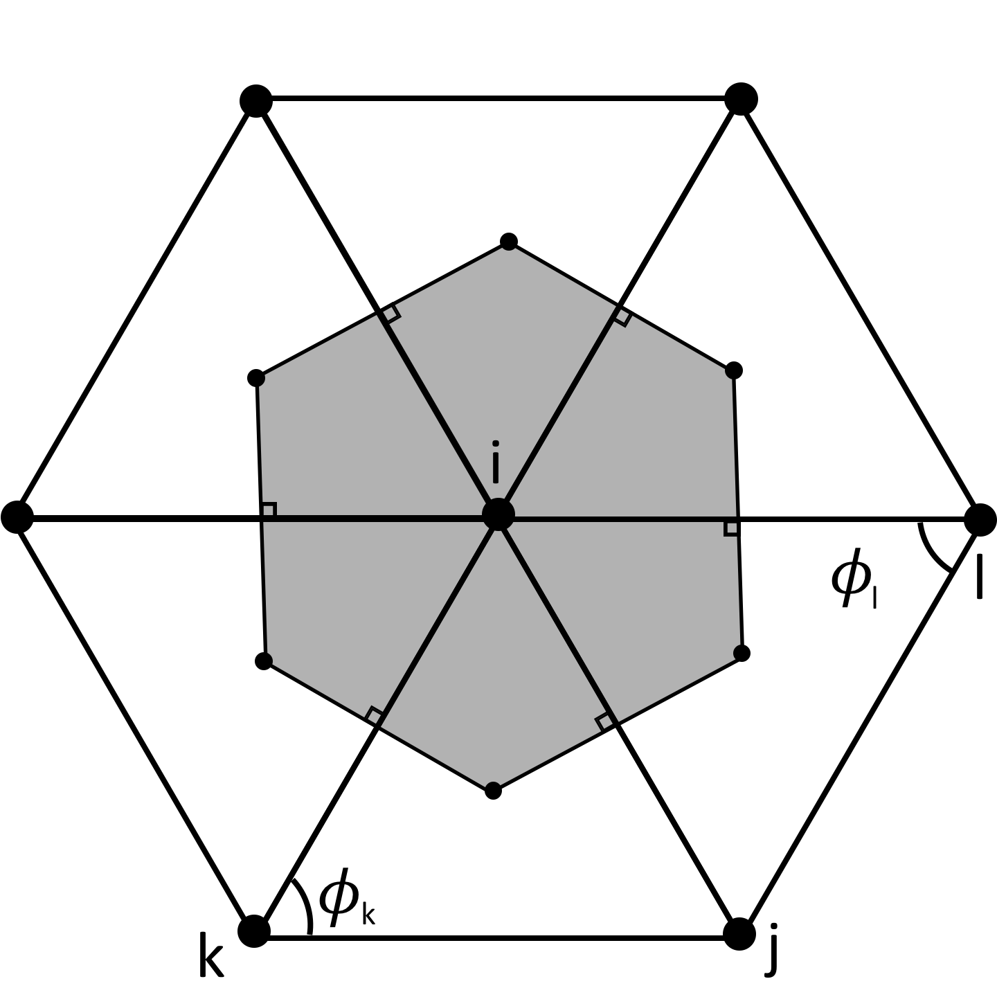
(b)

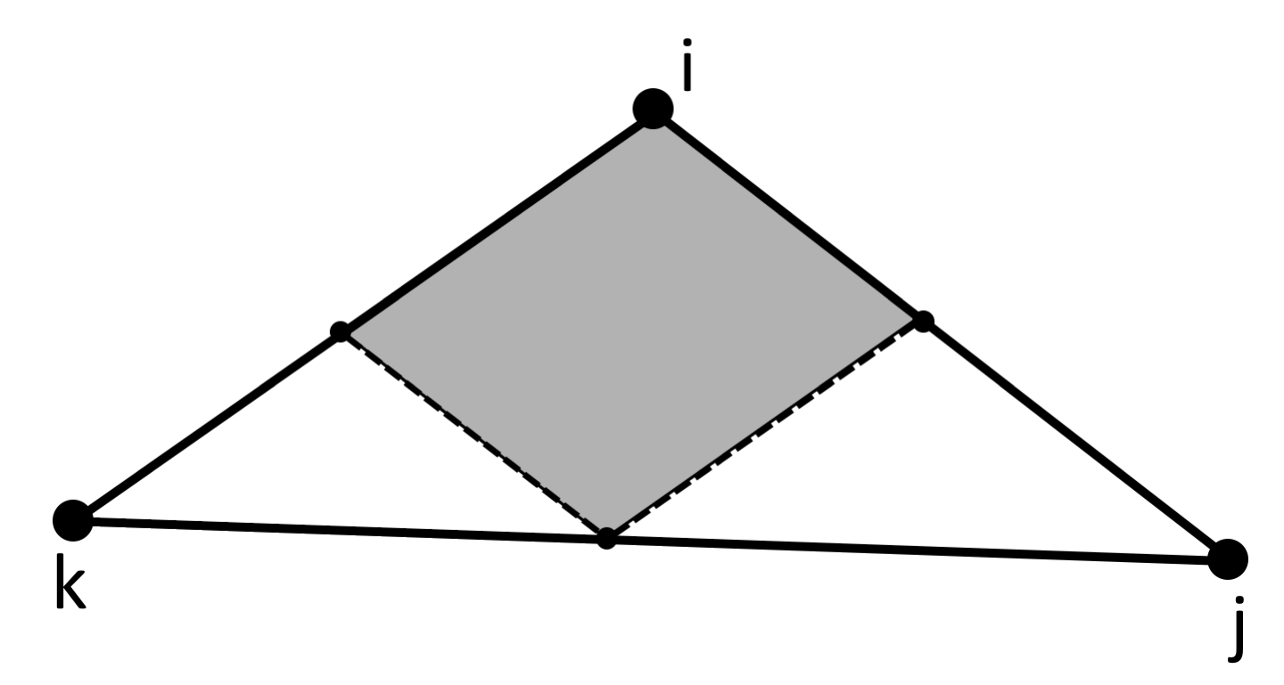
(c)

Figure 3: A sketch of area associated with vertex $i$. (a) Barycentric tessellation of area using barycentric centers of each triangle around vertex $i$ by scheme B. (b) Voronoi tessellation of area using circumcenters of each triangle around vertex $i$ by scheme C and D. (c) Tessellation of an obtuse triangle using the middle point of each edge by scheme D.

With the definitions of local mean curvature and area in Eqs. (21) and (22), we may calculate the three moments defined in Eq. (12). The expression for the discrete force is given in C and it consists of three primitive derivatives

$$\frac{\partial l_{e}}{\partial{\bf x}_{m}},\quad\frac{\partial\theta_{e}}{\partial{\bf x}_{m}},\quad\frac{\partial A^{t}}{\partial{\bf x}_{m}}.$$ (23)

3.4 Scheme C

This scheme was proposed by Gompper & Kroll [3] to simulate a triangular network of fluid vesicles and later applied to model general membranes [35]. Its discrete definition of Laplace-Beltrami operator reads [53, 54, 4]:

$$\left(-\nabla^{2}_{s}w\right)_{i}=\frac{\sum^{N^{i}_{e}}_{e:\left<i,j\right>}\left(\cot\phi_{k}+\cot\phi_{l}\right)\left(w_{i}-w_{j}\right)}{2A^{voro}_{i}},$$ (24)

where $w$ is an arbitrary function. The Voronoi area associated to vertex $i$ indicated on Fig. 3(b) and is defined as

$$A^{voro}_{i}=\frac{1}{8}\sum^{N^{i}_{e}}_{e:\left<i,j\right)}\left(\cot\phi_{k}+\cot\phi_{l}\right)\left|{\bf x}_{i}-{\bf x}_{j}\right|^{2}.$$ (25)

If we consider the discrete counterpart of an expression for mean curvature known from differential geometry, that is,

$$H_{i}=\frac{1}{2}\left(\nabla^{2}_{s}{\bf x}\right)_{i}\cdot{\bf n}_{i},$$ (26)

and take function $w$ as the surface coordinate ${\bf x}$ in Eq. (24), we have an explicit discrete definition of $H_{i}$. When only the Helfrich energy/force with $H_{0}=0$ is considered, $H^{2}_{i}=\frac{1}{4}\left[\left(\nabla^{2}_{s}{\bf x}\right)_{i}\right]^{2}$ [3, 40, 55], as $\nabla^{2}_{s}{\bf x}$ is along ${\bf n}$ direction. However, for the general energy/force in the SC and BC/ADE models considered in this work, we need an explicit discrete definition of ${\bf n}_{i}$. We consider a discrete ${\bf n}_{i}$  [56, 57, 40]. where the unit normal vector for vertex $i$ is the sum of neighboring normal vectors weighted by incident angles [56, 57].

$${\bf n}_{i}=\frac{\sum^{N^{i}_{t}}_{t:\left<i,j,k\right>}\phi^{t}_{i}{\bf u}^{t}}{|\sum^{N^{i}_{t}}_{t:\left<i,j,k\right>}\phi^{t}_{i}{\bf u}^{t}|},$$ (27)

where $\phi^{t}_{i}$ is the angle at vertex $i$ of triangle $t:\left<i,j,k\right>$, ${\bf u}^{t}$ is the unit normal vector of triangle $t$.

With the definitions of local mean curvature and area in Eqs. (26) and (25), we calculate the three moments in Eq. (12), and the total energy in Eq. (13). The expression of the force is given in D.

3.5 Scheme D

This scheme was derived from an effort of developing a ”unified and consistent set of flexible tools to approximate important geometric attributes, including normal vectors and curvatures on arbitrary triangle meshes” [4]. It has been adopted by several groups to study the bending mechanics of the minimal model for vesicles and RBCs [58, 38, 40]. The definition of the discrete Laplace-Beltrami operator reads as [4],

$$\left(-\nabla^{2}_{s}w\right)_{i}=\frac{\sum^{N^{i}_{e}}_{e:\left<i,j\right>}\left(\cot\phi_{k}+\cot\phi_{l}\right)\left(w_{i}-w_{j}\right)}{2A^{mix}_{i}},$$ (28)

which has almost identical expression as the one from scheme C, except that the area for vertex $i$ is calculated as a mixture of two approaches [4](see Fig. 3(c)).If the triangle $t:<i,j,k>$ is non-obtuse then local areas $A_{i}$, $A_{j}$, and $A_{k}$ on three vertices take the contribution from Voronoi tessellation of $A^{t}$, If the triangle $t:<i,j,k>$ is obtuse then the tessellation relies on the middle point of each edge. Therefore, the triangle $t:<i,j,k>$ contributes $A^{t}/2$ to $A_{i}$, and $A^{t}/4$ to $A_{j}$ and $A_{k}$ each [4].

The key difference of scheme D from the other three schemes is in terms of the force calculation. The force density of scheme D relies on the variational expression in Eq. (9) or (10). Once the discrete mean curvature $H_{i}$ is calculated at each vertex, we apply Eq. (28) second time on discrete values of $H$ to get $(\nabla^{2}_{s}H)_{i}$. Furthermore, only scheme D needs a discrete definition of Gaussian curvature at vertex $i$ [59]

$$G_{i}=\frac{1}{A^{mix}_{i}}\left(2\pi-\sum^{N^{i}_{t}}_{t:\left<i,j,k\right>}\phi^{t}_{i}\right),$$ (29)

which employs all incident angles around vertex $i$ and its area definition. Therefore, each discrete force density in Eq. (8) is readily available and thereafter the total force density can also be obtained.

4 Results

We present the results of the comparative study for all four schemes and the proposed extensions. We distinguish applications on prescribed shapes and on dynamically equilibrated shapes.

4.1 Prescribed configurations: sphere and bi-concave oblate

We first examine the performance of the four schemes on the calculation of the Helfrich energy for a sphere and a biconcave oblate described by an empirical function [60] using $\kappa_{b}=1$ and $h_{0}=0$ . The sphere is approximated with an icosahedron and higher resolutions are obtained by applying Loop’s subdivision scheme [61] for triangulated meshes with $N_{t}=80$, $320$, $1280$, $5120$. The same resolution is obtained for a biconcave oblate by transforming the surface coordinates of the sphere to the empirical function of the biconcave shape. We present the results in Fig. 4 verifying the total energy converges (albeit to different values !) with increasing the number of triangles. For the sphere, all four schemes converge with increasing the number of triangles (Fig.  4(a)). The first-order approximation of scheme A deviates significantly from scheme A when $N_{t}<320$ when the angle $\theta$ between two neighboring triangles is not small. Schemes B, C and D converge to a correct value $8\pi$.

For the biconcave-oblate configuration we compute the reference solution analytically (see E). We find that all four schemes converge to the reference solution with increasing number of triangles ( Fig.  4(b)). We note that the results from the first-order approximation for scheme A deviate significantly from those of the complete scheme A for $N_{t}<1280$. Moreover, with $\tilde{\kappa}_{b}=\sqrt{3}\kappa_{b}$, scheme A and its simplified version again converge to a higher value than the one given by the reference solution. The value of the total energy for the prescribed shapes does not depend on the details of the triangulated mesh, as long as the mesh is regular.

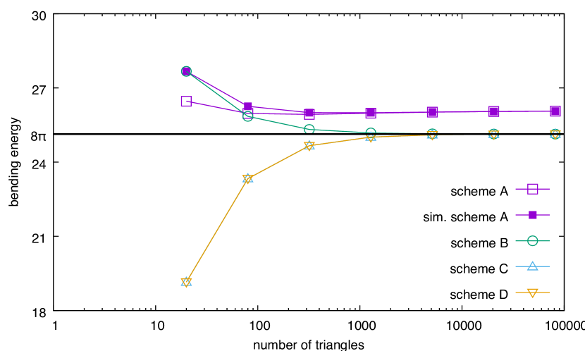
(a)

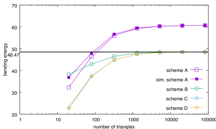
(b)

Figure 4: Helfrich energy from four discretization schemes with $\kappa_{b}=1$ and $h_{0}=0$. (a) sphere; (b) biconcave oblate. For scheme A, $\tilde{\kappa}_{b}=\sqrt{3}\kappa_{b}$ and $\theta_{0}=0$, and solid square is from the simplified scheme A with first-order approximation.

(a)

(b)

Figure 5: Total Helfrich and area-difference elasticity (ADE) energy from three discretization schemes with $\kappa_{b}=1$, $h_{0}=-0.5$, $\alpha=2/\pi$ and $d=D/R=0.001$. $E^{H}$; Helfrich energy; $E^{AD}$: ADE energy. (a) sphere with $\Delta a_{0}=\Delta A_{0}/(4\pi RD)=-1$; (b) biconcave oblate with $\Delta a_{0}=\Delta A_{0}/(4\pi RD)=-0.7$.

Subsequently, we compute total energy with $\kappa_{b}=1$, $h_{0}=-0.5$ and $\alpha=2/\pi$ using scheme B, C and D ( Fig. 5). All three schemes converge with increasing the number of triangles to the reference values. As shown in Fig.  5, for low resolution $N_{t}<320$, scheme B deviates much less than schemes C and D from the reference values.

(a)

(b)

Figure 6: Energy density versus radial distance of vertices from axis of symmetry for a biconcave oblate with $\kappa_{b}=1$ and $h_{0}=0$. For scheme A and its simplified version $\tilde{\kappa}_{b}=\sqrt{3}\kappa_{b}$ and $\theta_{0}=0$. (a) $N_{t}=1280$; (b) $N_{t}=5120$ and plotted for clarity with every $16$ vertices in arbitrary order.

Furthermore, for the biconcave-oblate configuration we plot energy density versus the radial distance from the axis of symmetry ( Fig. 6). Results from scheme B, C and D with $N_{t}=1280$ coincide with the reference line except a few discrepancies, which disappear with high resolution $N_{t}=5120$. Scheme A and its simplified version show no difference, but deviate from the reference values. Increasing the resolution from $N_{t}=1280$ to $5120$ does not improve the results of scheme A or those of its simplified version. The results indicate that scheme A is not an effective discretization of the Helfrich energy,consistent with the findings of two recent works [38, 40].

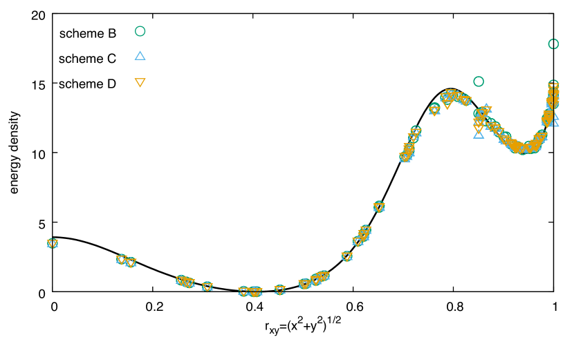
(a)

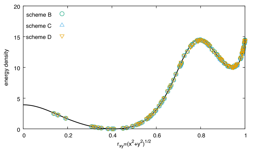
(b)

Figure 7: Energy density versus radial distance of vertices from axis for a biconcave oblate with $\kappa_{b}=1$ and $h_{0}=-0.5$. (a) $N_{t}=1280$; (b) $N_{t}=5120$ and plotted for clarity with every $16$ vertices in arbitrary order.

Finally, we examine the energy density for the Helfrich energy with $h_{0}\neq 0$, as computed by schemes B, C and D. We present the results in Fig. 7. All three schemes capture accurately the profile of the reference line. Some outliers showing for $N_{t}=1280$ also disappear for higher resolution $N_{t}=5120$. Note that the ADE energy is non-local and has only one global value, which was already presented in Fig. 5.

4.2 Numerical results on equilibrium shapes

Here we consider the equilibrium shapes of a closed membrane. The energy minimization process is initialized from a prescribed shapes such as a sphere, prolate and oblate ellipsoids, or from the equilibrium shape (e.g. stomatocyte) of an optimization using different parameters.

The minimization process relies on the calculation of the forces corresponding to the associated energy. The energy and the force are both calculated on the triangulated mesh. We set $\kappa_{b}=0.01$ and $\alpha=2/\pi$ [42, 28]. We penalize the constraints on global area with $\kappa_{ag}=2$ (F) and volume with $\kappa_{v}=1$ (G) [31, 48, 36, 37]. We also add an in-plane viscous damping force between any two neighboring vertices connected by an edge in order to dampen the kinetic energy. To explore the energy landscape efficiently, we also add a stochastic force of white noise between any two neighboring vertices connected by an edge. The pair of viscous and stochastic forces between vertices resemble the pairwise thermostat [62], which conserves momenta and has a proper thermal equilibrium. The time integration is performed by the explicit velocity Verlet method. As the minimization evolves, the configuration of the triangulated mesh may deteriorate, e.g., elongate in on direction or generate obtuse angles. We remedy this mesh distortion by introducing two regularization schemes: by introducing a constraint on the local area with $\kappa_{al}=1$ as penalization (F) [48, 36, 37] or by triangle equiangulation [63]. We note that as we perform multiple runs from different initial shapes we may reach different local minima of the energy landscape. Thereafter, we select the smallest among all available local minima as the global minimum, that is, the ground state.

4.2.1 The minimal model

We first consider the minimal model described by Helfrich energy with $h_{0}=0$  [5, 25]. As the equilibrium shapes are axi-symmetric, the computations are reduced to solving two-dimensional Euler-Lagrangian ODEs. We aim to reproduce the known phase-diagram with configurations and energies, in particular for small reduced volumes [64]. Furthermore, as the minimal model is widely used to simulate vesicles and RBCs we examine the performance of all four schemes in this situation.

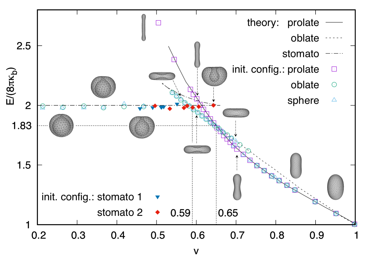
Figure 8: Local energy minima and corresponding shapes at different branches in the minimal model: symbols for energy and some selective configurations are by scheme B with $N_{t}=1280$. The axis of symmetry for each configuration always points upwards. Reference lines of theory are adapted from Seifert et al. [25].

We present the phase diagram of the reduced volume $v$ and the normalized energy of the vesicles as generated by scheme B in Fig. 8. Results from schemes A, C and D are quite similar to those obtained from scheme B, so in the following we only emphasize their discrepancies. We adopt the reference lines from the work of Seifert et al [25] and denote our results with symbols. Each symbol corresponds to the energy minima as obtained from our minimization procedure.

The reference lines correspond to three types of configurations. With decreasing $v$ in the prolate branch, the shape changes from sphere to prolate, dumbbell, and long caped cylinder. With decreasing $v$ in the oblate branch the shape changes from a sphere to a famous biconcave-oblate shape at around $v=0.6$. For $v=0.51$ the oblate branch bifurcates to form two stomatocyte sub-branches. One sub-branch has constant energy for $0<v<0.66$ while the other has energy which depends on volume.

The simulation results denoted by symbols in Fig. 8, are obtained by three initial shapes: sphere, prolate and oblate ellipsoids. The volume for the initial prolate and oblate ellipsoids are the same as that of the target $v$. However, the prolate and oblate branches generated in this work are different from the reference work [25]. The reference restricts the prolate branch to only prolate-like shapes and the oblate branch to oblate-like shapes. Here, we do not impose such constraint on the shape during the minimization procedure. More specific, all the squared symbols are from initial shape of prolates and they all stay on the prolate branch when reaching the local energy minimum. Similarly, all the circle symbols are from initial shapes of oblates, with the corresponding $v$, that stay on the oblate branch for $v\lesssim 0.75$ and jump onto the prolate branch for $v\gtrsim 0.75$. This results corroborates an earlier finding [41] where the oblate branch is only locally stable for $v\lesssim 0.75$. For the minimization from a spherical initial shapes (up triangle symbols), the energy minima are found on the prolate branch for $v\gtrsim 0.75$, on the oblate branch for $v\lesssim 0.65$ and scatter between prolate and oblate branches for $0.65\lesssim v\lesssim 0.75$.

For the constant energy sub-branch of the stomatocyte, we can not explore the partial ($v\gtrsim 0.51$) energy landscape directly. Therefore, we take two final shapes of stomatocyte, which are obtained by minimization with initial shapes of oblates. One final shape is from $v=0.4$ and the other is from $v=0.45$. We use these two shapes as initial shapes to run minimization procedure with targeted reduced volume $v$ ranging from $0.45$ to $0.66$. The results from $v=0.4$ are denoted with solid down triangles while from $v=0.45$ are solid diamonds.

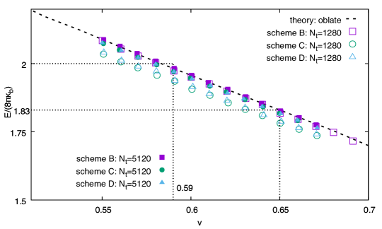
Figure 9: Resolution study for schemes B, C and D with $N_{t}=1280$ and $5120$: initial shapes are sphere. The reference lines of theory are adapted from Fig. 8 in Seifert et al. [25].

We demonstrate the convergence of the minimization process for the calculated energies, by examining the results in $0.55<v<0.7$, as this range contains the regime of oblate-like biconcave shapes ($0.59<v<0.65$) that is relevant for the simulations of RBCs. We present results from schemes B, C and D with two resolutions $N_{t}=1280$ and $5120$ in Fig. 9. It is apparent that scheme B is superior, as it already captures the reference values with $N_{t}=1280$, whereas scheme C and D reproduce the same results with $N_{t}=5120$. Moreover, the energies at delimiting points, that is, $2$ for $v=0.59$ and $1.83$ for $v=0.65$ are reproduced quite well by all three schemes. The minimal energies computed by scheme A are removed, as they are completely out of range. This should not be surprising, given its performances on two static configurations in section 4.1. Nevertheless, we present the equilibrium shapes by scheme A along with the other three schemes.

Table 2: Equilibrium shapes of the minimal model: comparison among four schemes for $0.65<v<1$ with $N_{t}=1280$.

$v$	$0.67$	$0.75$	$0.85$	$0.95$
A
B
C
D

We select four equilibrium configurations in the prolate-like/dumbbell/cigar regime with $0.65<v<1$ generated by the four schemes with $N_{t}=1280$ in Table 2. We find very small differences in the shapes obtained by the four schemes.

Table 3: Equilibrium shapes of the minimal model: comparison among four schemes for $0.59<v<0.65$ with $N_{t}=1280$.

$v$	$0.6$	$0.62$	$0.64$
A
B
C
D

However, in the biconcave-oblate regime for $0.59<v<0.65$ ( Table 3), shapes obtained by scheme A are different from those of the other three schemes, consistent with recent work [55]. With an oblate-like biconcave shape as initial shapes, we reproduce the same sequence of shapes by scheme A as those shown in the supplementary movie of [55]. However, the run time of [55] is too short to observe the equilibrium configurations. Moreover, the final (local) equilibrium shape by scheme A is also dependent on the initial shapes. Each shape by scheme A in Table 3 is selected as the smallest energy among steady states of three minimizations, each of which has one initial shapes among sphere, prolate and oblate. The equilibrium shapes by scheme A are always prolate-like/dumbbells/cigars, which are completely different from the analytical results in the reference study [25]. Schemes B, C, and D all produce the biconcave oblates with no distinct differences among them.

Table 4: Equilibrium shapes of the minimal model: comparison among four schemes for $0.25\leq v\leq 0.45$.

$v$	$0.25$	$0.3$	$0.35$	$0.4$	$0.45$
B: $N_{t}=320$
B: $N_{t}=1280$
B: $N_{t}=5120$
C: $N_{t}=1280$
C: $N_{t}=5120$

At smaller reduced volume $v<0.59$, scheme A does not generate stomatocyte, but always ends up with vesiculations, that is, two sphere like shapes connected via thin tubes (not shown here). Schemes B and C generate equilibrium shapes consistent with what is expected by the reference study as shown in Table 4 for two and three different resolutions. Scheme B is stable even at low resolution of $N_{t}=320$, although the equilibrium shapes are not as accurate. Especially for $v=0.25$ and $0.3$, scheme B with $N_{t}=320$ does not lead to the proper stomatocyte. Instead the two spheres are connected externally via a line segment, which can be seen from two orthogonal views (the first two entries in the first row of Table 4). These two shapes are caused by the under-resolved neck connecting the two spheres at this low resolution. All equilibrium shapes generated by scheme B with$N_{t}=1280$ are accurately axi-symmetric stomatocyte and show virtually almost no difference from the results of $N_{t}=5120$. These results are comparable to the two-dimensional contours reported in the reference [25]. The results of scheme C are shown in the last two rows of Table 4 for $N_{t}=1280$ and $5120$. Especially for the most challenging case of $v=0.25$ considered here, scheme C leads to unphysical shapes. Even for $v\geq 0.3$, scheme C cannot separate the inner sphere from the outer sphere with a reasonable distance, due to poor resolution at the neck. The results of scheme D are very similar to those of scheme C as the minimization procedure evolves for each target $v$. However, once scheme D reaches quasi-steady state with a proper stomatocyte shape, the overall configuration oscillates and the shape becomes unstable. We tried to employ regularization and smoothing to stabilize scheme D, but we were unsuccessful. We speculate that since scheme D does not enforce the conservation of momentum or energy this may cause this instability. To the best of our knowledge, there are no reports from previous work using triangulated mesh to simulate such low volumes. The exact reason why scheme D is unstable remain obscure.

4.2.2 Spontaneous curvature model

We compute the minimal energies determined by the SC model and the corresponding equilibrium configurations. In particular, we consider two spontaneous curvature values $h_{0}=1.2$ and $1.5$ so that we can compare with results of Seifert et al [25]. The possible shapes generated by the SC model are still axi-symmetric. However, the SC model enables quite a few more configurations that are numerically challenging. These include pear-like shapes which break the up-down symmetry, budding transition with a narrow neck connecting the neighboring compartments of the same size, budding transitions with the neighboring compartments of different sizes, vesiculation where connection between the neighboring compartments of the same size is lost and vesiculation where connection between the neighboring compartments of different sizes is lost. There are also discontinuous transitions for $h_{0}\neq 0$, but the minimization procedure of exploring the energy landscape is quite similar to the case of $h_{0}=0$ and we do not elaborate on this finding here.

4.2.3 $h_{0}=1.2$

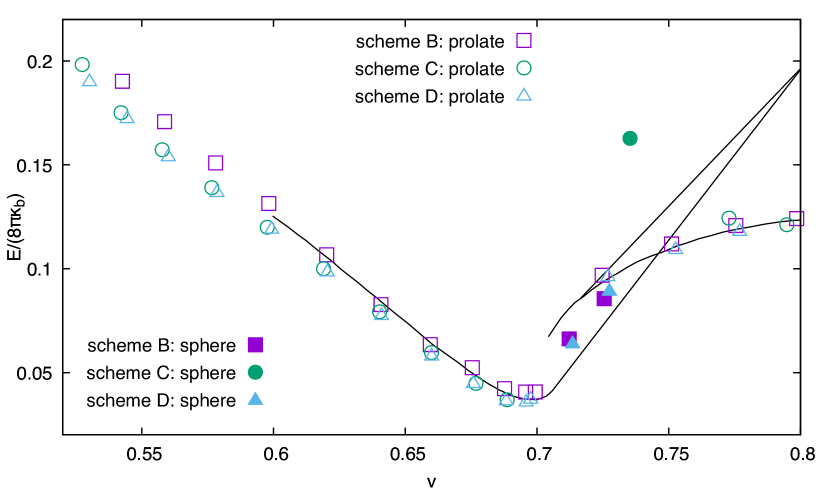
(a)

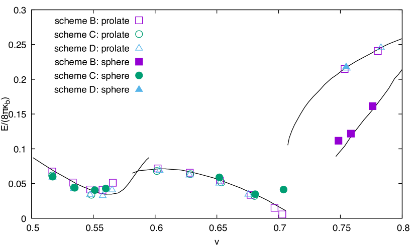
(b)

Figure 10: Minimized Helfrich energies for each $v$ by schemes B, C, and D with $N_{t}=1280$. The initial shapes are prolates or spheres . (a) $h_{0}=1.2$ and (b) $h_{0}=1.5$. The reference lines are adapted from Seifert et al. [25].

Table 5: Equilibrium shapes of the SC model $h_{0}=1.2$: comparison among three schemes for $0.52<v<0.8$ with $N_{t}=1280$.

$v$	$0.53$	$0.6$	$0.69$	$0.725-0.735$	$0.75$	$0.8$
B
C
D

We first consider $h_{0}=1.2$ and present the energy diagram in Fig. 10(a) and the representative equilibrium shapes in Table 5. The references are adapted from Seifert et al. [25]. For the regime $v<\sqrt{2}/2\approx 0.71$, all three schemes accurately capture the shapes of necklace (with two necks) at $v=0.53$, dumbbells at $v=0.6$ and budding at $v=0.69$, as shown in the first three columns of Table 5. The minimum energies in this regime computed by the three schemes are also quite close to the reference line. Especially scheme B accurately reproduces the energy line with $N_{t}=1280$ as shown in the left part of Fig. 10(a). For the regime $v\gtrsim 0.75$, we expect prolate/dumbbell shapes as suggested by the reference. All three schemes B, C and D are able to get the minimum energies accurately as shown in the right part of Fig. 10(a), and to generate the expected shapes comparable to the reference (see figure 12 of Ref. [25]) as shown in the last two columns of Table 5. The most challenging regime resides in $0.71\lesssim v\lesssim 0.75$, since there are multiple local minima and the energy diagram bifurcates. However, all three schemes are able to produce the budding, where there is only one very thin neck connecting the two compartments of different sizes. For this very extreme regime, we do not expect accurate computation on the minimum energy. However, the energies by scheme B and D are still surprisingly close to the reference, whereas the scheme C is completely off due to the poor representation of the narrow neck with only a couple of triangles.

4.2.4 $h_{0}=1.5$

Table 6: Equilibrium shapes of SC model $h_{0}=1.5$: comparison among three schemes for $0.52\leq v\leq 0.78$ with $N_{t}=1280$.

$v$	$0.52$	$0.56$	$0.65$	$0.7$	$0.76$	$0.78$
B
C					NA	NA
D				NA	NA	NA

Computations for the case of $h_{0}=1.5$ are even more challenging as, besides budding transitions, vesiculations are also expected. For the regime $v\lesssim 0.58$, all three schemes are able to generate necklaces as shown in the first two columns in Table 6 and compute minimum energy accurately as shown on the left part of Fig. 10(b). There is notable discrepancy for the equilibrium shape generated by scheme C at $v=0.56$, as it cannot sustain the axis-symmetry due to its inability to resolve the narrow necks of the budding shapes. For the regime $0.6\lesssim v\lesssim 0.71$, all three schemes can generate dumbbell shapes at equilibrium, for example, at $v=0.65$. However, only scheme B can generate vesiculation of two spheres of equal size expected from the reference [25], as shown by one example of $v=0.7$ on Table 6. Scheme C at $v=0.7$ may generate vesiculation, but the two compartments do not have equal size and the energy differs from the reference. Perhaps the regime of $v\gtrsim 0.75$ is the most challenging one, since the two compartments are expected to have up-down symmetry breaking for the vesiculation. We find that both schemes C and D to run stably in this regime of vesiculations. On the contrary, scheme B delivers the correct results with a satisfactory accuracy on both the energy values and configurations.

To summarize this section, scheme B with $N_{t}=1280$ is able to generate the whole spectrum of equilibrium shapes including dumbbells, necklaces, even buddings and vesiculations where only a couple of triangles are connecting different compartments. Furthermore, the corresponding energy value for each equilibrium shape is very accurate in comparison with the reference value. Both schemes C and D with $N_{t}=1280$ run into troubles when budding or/and vesiculations are expected. With higher resolutions $N_{t}=5120$, neither scheme C nor D show significant improvement (results not presented herein).

4.2.5 Bilayer-couple model

We consider the phase diagram of the BC model which can be realized by taking $\alpha\rightarrow\infty$ in Eq.  (5) so that the area-difference elasticity becomes a quadratic penalization. In this model, there are two non-dimensional parameters $v$ and $\Delta a$. We consider the BC model before presenting results from the complete ADE model for a few reasons: 1. The BC model has only continuous phase transitions [13, 25]. 2. The equilibrium shapes and possible resultant $\Delta a$ in BC model contains those of the ADE model [6]. 3. The phase diagram of BC has two controlling parameters, one less than that of ADE model. 4. With $h_{0}=0$, we can focus on examinations the area-difference elasticity.

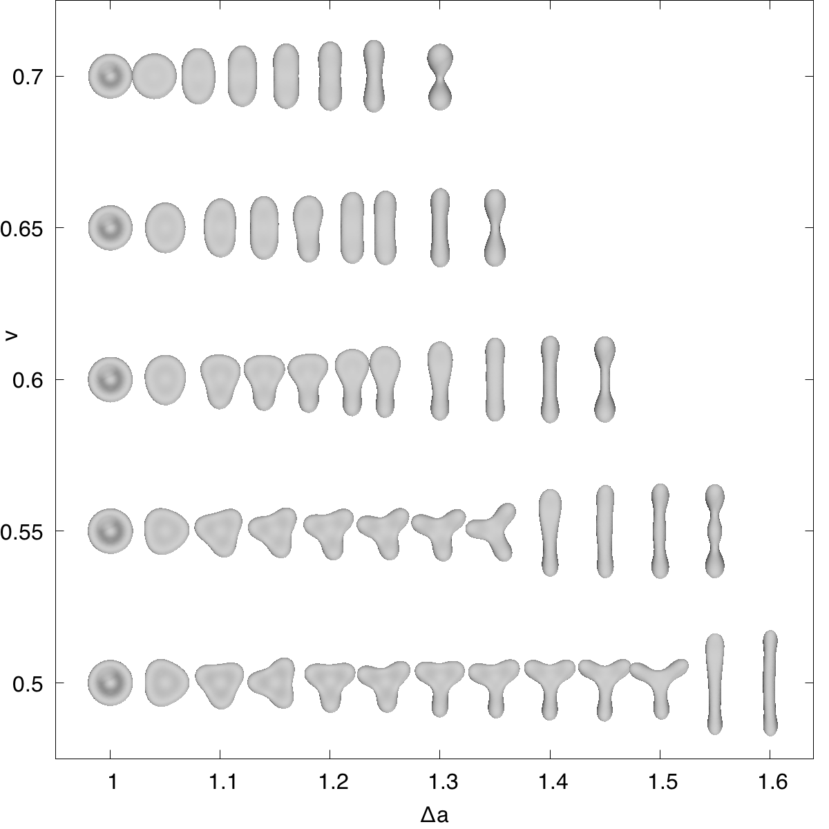
(a)

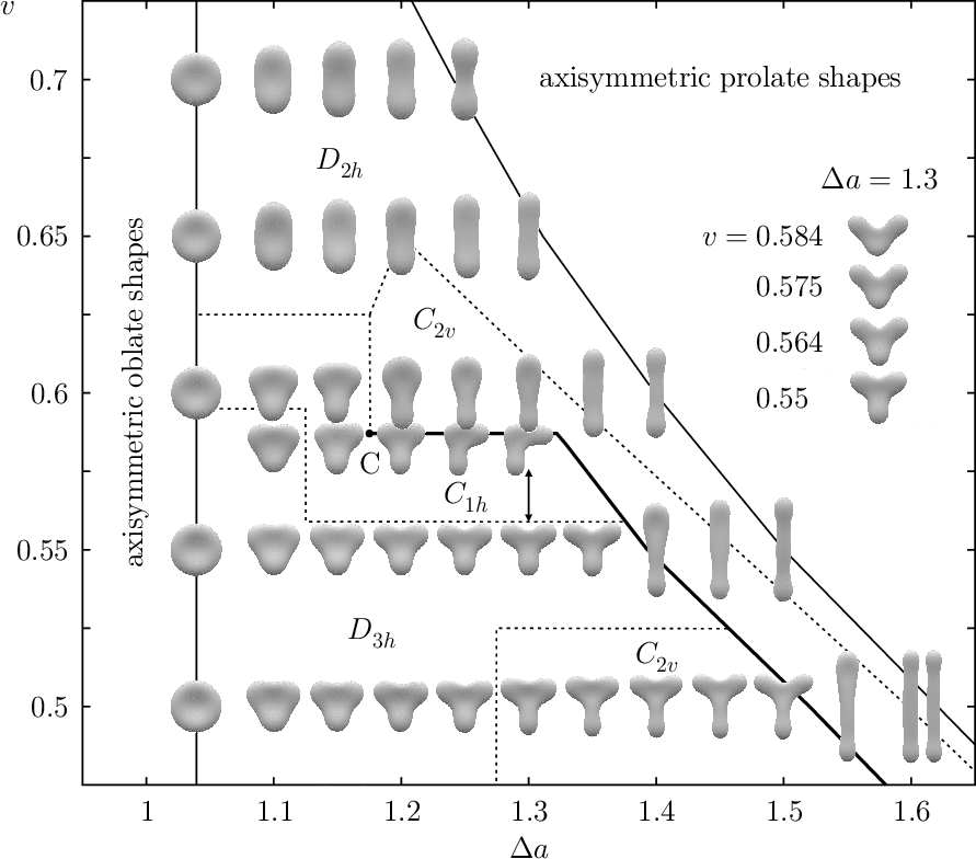
(b)

Figure 11: Equilibrium shapes of the BC model. The results are by scheme B with $N_{t}=1280$ (a) and comparable to the numerical work of Ziherl and Svetina [46] (b) (permission pending) and the experiments of Sakashita et al. [22] (not shown here).

We consider the same parameter ranges of $v$ and $\Delta a$ as in Ref. [46], where the program Surface Evolver was used [63]. We present our phase diagram by scheme B in Fig. 11, where almost each individual shape has one-to-one correspondence to the shape on Fig. 1 of Ziherl and Svetina [46]. As in the SC model, we obtain similar axi-symmetric shapes such as stomatocytes, prolate-like/dumbbells, budding necklaces. Different from the SC model, we obtain in addition many non-axisymmetric shapes from the constraint of the area difference between outer and inner leaflets. These shapes include elliptocytes (e.g., the fourth one at $v=0.7$ or $0.65$), rackets (e.g., the fifth one at $v=0.65$ and sixth one at $v=0.6$), triangle oblates with equal sides (e.g., the sixth one at $v=0.55$), and triangle oblates with unequal sides (e.g., the seventh one at $v=0.5$). All these shapes have been recently validated by experiments on self-assembled vesicles combined with image analysis [22].

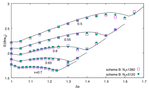
Figure 12: Minimal energies for the BC model. The references lines are adapted from Ziherl and Svetina [46].

Furthermore, we verify the corresponding energy values as shown in Fig. 12, where the reference values are adapted from Ziherl and Svetina [46]. We observe that energies computed by scheme B with $N_{t}=1280$ and $5120$ exhibit negligible discrepancies and they both follow closely the reference values. Therefore, we omit the equilibrium configurations generated with $N_{t}=5120$.

We have also computed the same phase diagram by scheme C and D with $N_{t}=1280$ and $5120$. However, scheme C and scheme D become unstable for certain values of $\Delta a$. We speculate that the vulnerability of scheme C is due to the definition of the discrete normal vector, which is not compatible with the discrete definition of the Laplace operator. We maintain that the instability of scheme D is due to its lack of conservation properties. We consider that a more rigorous investigations on scheme C and D are beyond the scope of this work.

4.3 Area-difference-elasticity model

Here we compute the total energy and force in the ADE model. For comparison, we consider as reference the work of Khairy et al.  [28], which employs spherical harmonics to represent the surface and calculate the total energy. Therefore, we take the same reduced volume $v\approx 0.642$ and $\alpha=2/\pi$, which represent the parameters of a normal RBC [42, 28].

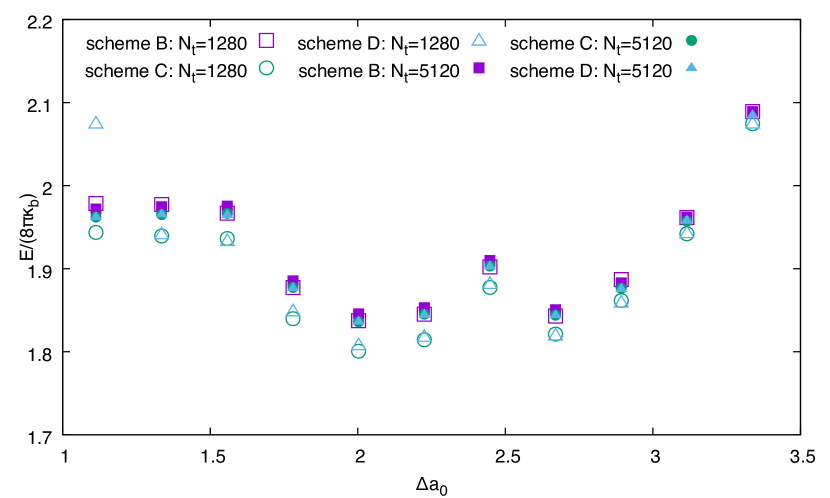
(a)

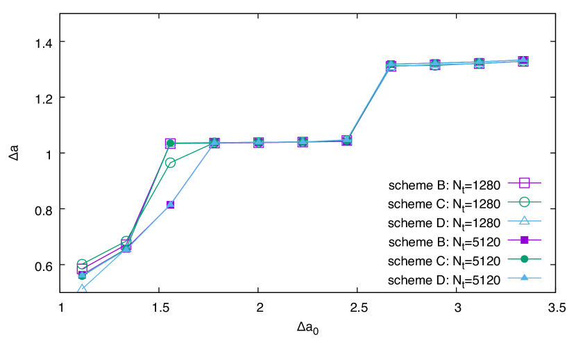
(b)

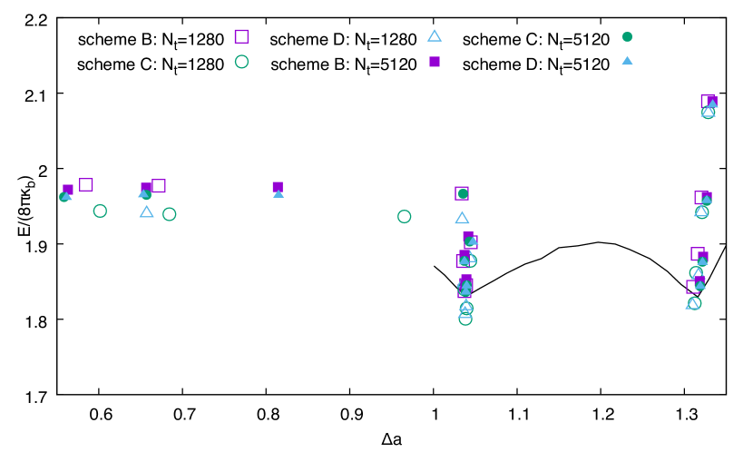
(c)

Figure 13: Minimal energies and area differences from ADE model: $\alpha=2/\pi$.

We present the energy versus reference area difference $\Delta a_{0}$ on Fig. 13(a), where we include results of all three schemes and each with two resolutions of $N_{t}=1280$ and $5120$. For each $\Delta a_{0}$ considered from $1$ to $3.5$, there is only small discrepancy between the schemes with a proper resolution, that is, scheme B with $N_{t}=1280$ and $5120$ and scheme C and D with $N_{t}=5120$. We present the resultant $\Delta a$ versus $\Delta a_{0}$ on Fig. 13(b) and observe that $\Delta a$ increases as $\Delta a_{0}$ for smaller $\Delta a_{0}\lesssim 1.75$. It stays almost at one plateau for $1.75\lesssim\Delta a_{0}\lesssim 2.5$ and at another plateau for $\Delta a_{0}\gtrsim 2.6$. Correspondingly, we plot again the energy versus the resultant $\Delta a$ on Fig. 13(c). We observe that the associated energies span among possible area differences for $\Delta a\lesssim 1$ and cluster at two discrete states of area differences for $\Delta a\gtrsim 1$. These characteristics of area differences and minimal energies reflect the possible equilibrium configurations of the vesicles, which will be presented next.

Table 7: Equilibrium shapes of the ADE model: comparison among four schemes for $N_{t}=1280$ and $5120$, $\alpha=2/\pi$. Both values of $\Delta a_{0}$ and $\Delta a^{\prime}_{0}$ are listed to compare with Khairy et al [28].

$\Delta a_{0}$	$1.11$	$1.34$	$1.78$	$2.34-2.56$	$3.34$
$100\Delta a^{\prime}_{0}$	$0.1$	$0.12$	$0.16$	$0.21-0.23$	$0.3$
B: $N_{t}=1280$
B: $N_{t}=5120$
C: $N_{t}=1280$
C: $N_{t}=5120$
D: $N_{t}=1280$
D: $N_{t}=5120$	NA

We present equilibrium configurations from scheme B, C and D with $N_{t}=1280$ and $5120$ in Table 7, where values of both $\Delta a_{0}$ and $\Delta a_{0}^{\prime}$ are considered, as the latter corresponds to the parameter in Fig 3c of Khairy et al [28]. With resolutions of $N_{t}=1280$, all schemes B, C and D resemble closely the results of the reference. As $\Delta a_{0}$ increases, we observe axi-symmetric stomatocytes with smaller height, as exemplified by the first two columns of Table 7. This regime corresponds to the first regime discussed above for Fig. 13, where $\Delta a$ grows as $\Delta a_{0}$ increases; As $\Delta a_{0}$ (and $\Delta a$) further increases, it enters to the second regime, where $\Delta a$ stays almost plateau. In this regime, we observe equilibrium shapes as biconcave-oblate and biconcave-elliptocyte, which are exemplified by the third and fourth columns of Table 7. In the last regime, $\Delta a$ stays flat and we observe prolate-dumbbells as shown for example in the last column of Table 7. These configurations of $N_{t}=1280$ agree with the work of Kairy et al [28]. However, with $N_{t}=5120$ the anisotropy of elliptocytes with $0.21\lesssim 100\Delta a^{\prime}_{0}\lesssim 0.23$ tends to disappear and the final configurations are less elongated. The results on elliptocyte with $N_{t}=5120$. We note that the difference between computed energies for $N_{t}=1280$ and $5120$ is very small as shown in Fig. 13. The results from the three different schemes are consistent with each other, which leads us to suspect that the number of terms in the spherical harmonics of the reference could be insufficient to resolve this subtle difference.

4.4 A dynamic simulation of of area-difference-elasticity model

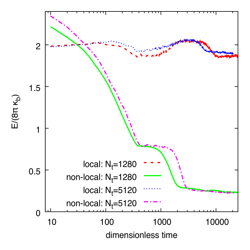
(a)

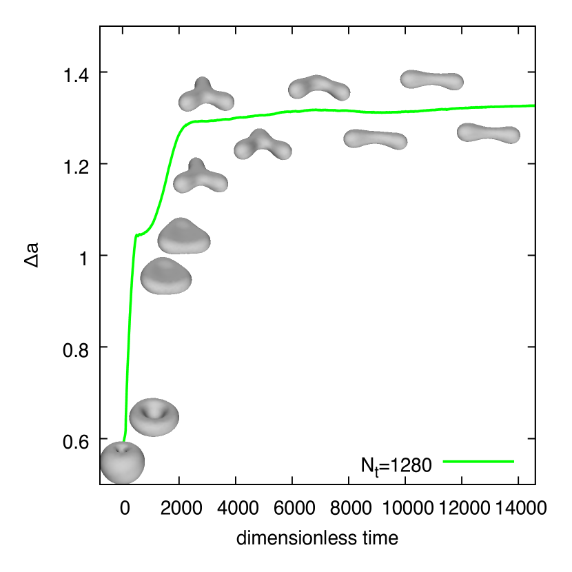
(b)

Figure 14: A dynamic trajectory of the ADE model with stomatocyte as initial shape and prolate-dumbbell as final shape. (a) Local and non-local energy versus time. (b) Area difference versus time and representative shapes along the trajectory. The representative shapes correspond to $t^{*}=0,250,750,1000,2000,3000,5000,7000,9000,11000,13000$ and $\Delta a=0.585,0.648,0.96,1.046,1.179,1.295,1.305,1.307,1.312,1.321,1.325$.

Finally, we present dynamic simulations of lipid bilayer membranes using the ADE model discretized by scheme B. We consider the same parameters as in section 4.3, that correspond to mechanics activities of a RBC. We start with a stomatoctye shape, which takes the final shape of the previous minimization procedure (see results of $\Delta a_{0}=1.11$ or $100\Delta a^{\prime}_{0}=0.1$ on Table 7). We set the reference area-difference as $\Delta a_{0}=3.34$ or $100\Delta a^{\prime}_{0}=0.3$.

We report the dynamic trajectories of local energy, non-local energy, area-difference and corresponding shapes on Fig. 14. The in-plane viscous damping force is orthogonal to the normal direction of the membrane surface and has negligible effects on the dynamic trajectories. However, a larger viscous force is needed to stabilize simulations with a higher resolution and therefore demands a smaller time step. The dynamic simulation arrives at the prolate-dumbbell shape, as shown on Fig. 14 in agreement with results on Fig. 13(a) and 13(b) and on Table 7, respectively, which are obtained from independent minimization procedures. From Fig. 14(a), we observe that the local energy does not change significantly over time, whereas the non-local energy decreases around ten fold. This confirms that the ADE is primarily responsible for the transformation of shapes. Comparing Fig. 14(b) with 13(b), we notice that the accessible states of $\Delta a$ are more abundant and even continuous in the dynamic simulation. Accordingly, there is a rich range of shapes including triangle oblates, curved-prolate-like shapes, and prolate-dumbbells, as represented on Fig. 14(b). These intermediate configurations are dynamic (non-equilibrium) and do not have a correspondence for the intermediate $\Delta a_{0}$ values on Table 7. Further comparing with the phase diagram of the BC model on Fig. 11, we also do not find corresponding equilibrium shapes for the same values of reduced volume and $\Delta a$. The small discrepancy between the energy trajectories of $N_{t}=1280$ and $5120$ are not surprising, as they start from slightly different values.

5 Summary

We have presented a comparative study of four bending models for lipid bilayer membranes and their respective discretization on triangulated meshes. The physical models are the minimal, spontaneous curvature (SC), bilayer-couple (BC) and area-difference elasticity (ADE) models and the four schemes are termed as scheme A, B, C, and D respectively.

We find that the total energies computed by scheme A on a prescribed sphere and biconcave oblate differ significantly from the analytical values. The energy computed by scheme A cannot be tuned to match the Helfrich energy for an arbitrary shape. For reduced volume $v>0.75$, scheme A is able to generate prolate-dumbbells at equilibrium, although the corresponding energies are inaccurate. However, for $0.59<v<0.65$, scheme A does not result in biconcave oblates as equilibrium shapes and it does not sustain the shape if it is given a biconcave oblate as the initial shape. Below $v<0.59$, scheme A has numerical artifacts of budding transitions and vesiculations. Finally, due to the lack of direct definition of mean curvature and local area, scheme A can not be directly extended to discretize the SC, BC, or ADE models.

The energies computed by scheme B, C and D on prescribed sphere and biconcave oblate match well the analytical values. However, the accuracy of the three schemes has a varying dependence on their resolution. On the phase diagram of the minimal model, for $v>0.59$, all three schemes produce prolate dumbbells and biconcave oblates as the equilibrium configurations. They also resolve well the critical energy values at $v=0.75$ and $0.65$ and $0.59$, with scheme B at $N_{t}=1280$ but scheme C and D at $N_{t}=5120$. However, for $v<0.59$, Scheme B produces stomatocytes as equilibrium configurations accurately with $N_{t}=1280$, where the inner sphere separates clearly from the outer sphere. Scheme C generates acceptable equilibrium configurations, but cannot maintain a clear physical separation between the inner and outer spheres. For the most challenging case of $v=0.25$, scheme C is in trouble to generate a physically correct configuration. A higher resolution of $N_{t}=5120$ does not help scheme C significantly on the overall equilibrium shape. Scheme D has stability issues in the regime of stomatocytes that may be attributed to its lack of explicit energy and momentum conservation.

We have also computed two slices ($h_{0}=1.2$ and $1.5$) of the phase diagram for the SC model. These are challenging benchmarks, as $h_{0}=1.2$ includes the budding transitions at equilibrium, while $h_{0}=1.5$ include both buddings and vesiculations. We observe that schemes B, C and D all capture accurately the budding process, but scheme C and D have difficulties to generate vesiculations. Furthermore, with the same resolution of $N_{t}=1280$ scheme B computes the energy more accurately than scheme C and D. Moreover, the energies computed by scheme C at budding transitions are completely off the reference values due to the poor representation of the configuration necks.

As a special case of the ADE model, we considered the BC model, where a constraint is imposed on the area difference between the two layers of lipid. We focus on the results of scheme B and reproduce the phase diagram for different resolutions. We find that results of scheme B are comparable to the reference on the equilibrium shapes and energy values, which were calculated by Surface Evovler. We have also considered the complete energy functional of the ADE model. We reproduce the sequence of stomatocytes, biconcave oblates, biconcave elliptocytes and prolate dumbbells by all three schemes, except for the extreme case of stomatocyte where scheme D runs into instability again. As the last demonstration, we consider a dynamic trajectory of the ADE model from stomatocyte to prolate-dumbbell. The values of local energy, non-local energy, and area-difference along the dynamic trajectory may also serve as reference for other researchers.

Our results indicate that it is a challenging task to compute accurately the bending energy and in particular forces on a triangulated mesh. However, due to its generality it is still a very promising path to pursue. At the same time we note the level set formulations introduced in [32] which incorporates some of the energy models presented in this work. We believe that this is a very promising direction to account for large membrane deformations and topological changes. Future work could be directed in comparing level set and triangulated surface representations.

In summary, the relatively simple formulation of scheme B, which bypasses definitions of Laplace-Beltrami operator and unit normal vectors, and instead defines the integral of mean curvature with respect to area, exhibits excellent accuracy, robustness, stability. Moreover as the the implementation of scheme B is also almost as simple as that of scheme A we suggest that it deserves to be more broadly investigated as an alternative for vesicle and RBC simulations. While scheme B is readily applicable to the minimal model, in this work we promote and extend its potentials to further resolve SC, BC and ADE models. With ADE model as the most accurate model for lipid bilayer membrane, we envision many numerical applications on vesicles and RBCs in a dynamic context.

Appendix A Force from variational calculus of energy

In differential geometry, the Cartesian coordinates ${\bf x}$ of a point on a surface may be expressed in terms of two independent parameters $u_{1}$ and $u_{2}$ as ${\bf x}={\bf x}(u_{1},u_{2})$. For further derivations, we introduce some definitions [65, 8]

$${\bf x}_{,i}=\frac{\partial{\bf x}}{\partial u_{i}},\quad{\bf x}_{,ij}=\frac{\partial^{2}{\bf x}}{\partial u_{i}\partial u_{j}},\quad g_{ij}={\bf x}_{,i}\cdot{\bf x}_{,j},$$

$$g^{ij}=\left(g_{ij}\right)^{-1}\quad or\quad g^{ij}g_{jl}=\delta^{i}_{l},\quad g=\det(g_{ij}),$$ (30)

where free index $i$ or $j$ is either $1$ or $2$, and summation convention applies to repeated index. Index $i$ after “,” denotes the partial derivative with respect to $u_{i}$. $g_{ij}$ is the covariant metric tensor and $g$ is its determinant. $g^{ij}$ is the contravariant metric tensor. An infinitesimal area is then

$$dA=g^{1/2}du_{1}du_{2}.$$ (31)

The parameterization of $u_{1}$ and $u_{2}$ are chosen in such a way the the normal direction

$${\bf n}=\frac{{\bf x}_{,1}\times{\bf x}_{,2}}{|{\bf x}_{,1}\times{\bf x}_{,2}|},$$ (32)

points inwards of a closed surface. Therefore, $H=\nabla\cdot{\bf n}/2$ is positive for a sphere.

For a small and continuous perturbation $\psi(u_{1},u_{2})$ along the normal direction ${\bf n}(u_{1},u_{2})$, the new position of the point on the parametric surface is given as

$${\bf x}^{\prime}(u_{1},u_{2})={\bf x}(u_{1},u_{2})+\psi(u_{1},u_{2}){\bf n}(u_{1},u_{2}).$$ (33)

Thereafter, the variations for $dA$ and $H$ are given as

$$\delta(dA) =2H\psi g^{1/2}du_{1}du_{2}=2H\psi dA,$$ (34)

$$\delta H =-(2H^{2}-G)\psi-\frac{1}{2}g^{ij}\left(\psi_{,ij}-\Gamma^{k}_{ij}\psi_{,k}\right)=-(2H^{2}-G)\psi-\frac{1}{2}g^{ij}\nabla_{i}\psi_{,j},$$ (35)

where $\Gamma^{k}_{ij}$ is the Christoffel symbol and $\nabla^{2}_{s}$ is the Laplace-Beltrami operator on the surface. We note a different sign convention used [8].

To have an explicit expression of $\delta E$, we need variational expressions for each moment. The variation of the zero moment simply reads as

$$\delta\mathcal{M}_{0} =\delta A=\int\delta(dA)=\int 2H\psi dA.$$ (36)

However, to calculate variations of the first and second moments we need some fundamental equalities. For any function $f(u_{1},u_{2})$ we have

$$\int f\psi_{,i}du_{1}du_{2}=-\int f_{,i}\psi du_{1}du_{2},\quad\int f\psi_{,ij}du_{1}du_{2}=\int f_{,ij}\psi du_{1}du_{2},$$ (37)

which can be readily proven via integration by parts. We further notice

$$\left(g^{1/2}g^{ij}f\right)_{,ij} =\left[\left(g^{1/2}g^{ij}\right)_{,j}f\right]_{,i}+\left(g^{1/2}g^{ij}f_{,j}\right)_{,i},$$ (38)

$$\left[\left(g^{1/2}g^{ij}\right)_{,j}f\right]_{,i} =-g^{1/2}g^{ij}\left(\Gamma^{k}_{ij}f\right)_{,k},$$ (39)

$$g^{-1/2}\left[g^{1/2}g^{ij}f_{,j}\right]_{,i} =\nabla^{2}_{s}f.$$ (40)

Therefore,

$$\int fg^{ij}\left(\psi_{,ij}-\Gamma^{k}_{ij}\psi_{,k}\right)dA$$

$$= \int fg^{ij}\left(\psi_{,ij}-\Gamma^{k}_{ij}\psi_{,k}\right)g^{1/2}du_{1}du_{2}$$

$$= \int\left[\left(g^{1/2}g^{ij}f\right)_{,ij}+\left(g^{1/2}g^{ij}\Gamma^{k}_{ij}f\right)_{,k}\right]\psi du_{1}du_{2}$$

$$= \int\left\{\left[\left(g^{1/2}g^{ij}\right)_{,j}f\right]_{,i}+\left(g^{1/2}g^{ij}f_{,j}\right)_{,i}-\left[\left(g^{1/2}g^{ij}\right)_{,j}f\right]_{,i}\right\}\psi du_{1}du_{2}$$

$$= \int\left(g^{1/2}g^{ij}f_{,j}\right)_{,i}\psi du_{1}du_{2}$$

$$= \int\nabla^{2}_{s}fg^{1/2}du_{1}du_{2}=\int\nabla^{2}_{s}fdA,$$ (41)

Eq. (37) is applied from the second to the third line. Eqs. (38) and (39) are applied from the third to the fourth line. Eq. (40) is applied from the fifth to the sixth line.

The variation of the first moment is readily obtained as

$$\delta\mathcal{M}_{1} =\int\left[\delta HdA+H\delta(dA)\right]$$

$$=\int\left[-(2H^{2}-G)\psi-\frac{1}{2}g^{ij}\left(\psi_{,ij}-\Gamma^{k}_{ij}\psi_{,k}\right)+2H^{2}\psi\right]dA$$

$$=\int\left[G\psi-\frac{1}{2}g^{ij}\left(\psi_{,ij}-\Gamma^{k}_{ij}\psi_{,k}\right)\right]dA$$

$$=\int\left(G-\frac{1}{2}\nabla^{2}_{s}1\right)\psi dA=\int G\psi dA,$$ (42)

where Eq. (41) is applied from the third to the fourth line. The variation of the second moment is also readily derived as

$$\delta\mathcal{M}_{2} =\int\left[2H\delta HdA+H^{2}\delta(dA)\right]$$

$$=\int\left[-2H(2H^{2}-G)\psi-Hg^{ij}\left(\psi_{,ij}-\Gamma^{k}_{ij}\psi_{,k}\right)+2H^{3}\psi\right]dA$$

$$=\int\left[-2H(H^{2}-G)\psi-Hg^{ij}\left(\psi_{,ij}-\Gamma^{k}_{ij}\psi_{,k}\right)\right]dA$$

$$=\int\left[-2H\left(H^{2}-G\right)-\nabla^{2}_{s}H\right]\psi dA,$$ (43)

where Eq. (41) is applied from the third to the fourth line.

Since the perturbation $\psi$ is continuous, small and arbitrary, the integrand must be the density of virtual work along the normal direction. Therefore, the magnitudes of the virtual force density due to the three moments read as

$$\mathcal{F}_{0}=2H,\quad\mathcal{F}_{1}=G,\quad\mathcal{F}_{2}=-2H\left(H^{2}-G\right)-\nabla^{2}_{s}H,$$ (44)

and they all act along the normal direction ${\bf n}$. These results also corroborate another two recent derivations following different routes [43, 66].

The variation of energy of Eq. (7) read as

$$\delta E =2\kappa_{b}\delta\mathcal{M}_{2}+\frac{4\alpha\kappa_{b}\pi}{A}\mathcal{M}_{1}\delta\mathcal{M}_{1}-\frac{2\alpha\kappa_{b}\pi}{A^{2}}\mathcal{M}^{2}_{1}\delta A-4\kappa_{b}H_{0}\delta\mathcal{M}_{1}$$

$$-\frac{2\alpha\kappa_{b}\pi}{A}\frac{\Delta A_{0}}{D}\delta\mathcal{M}_{1}+\frac{2\alpha\kappa_{b}\pi}{A^{2}}\frac{\Delta A_{0}}{D}\mathcal{M}_{1}\delta A+2\kappa_{b}H^{2}_{0}\delta A-\frac{\alpha\kappa_{b}\pi}{2A^{2}}\left(\frac{\Delta A_{0}}{D}\right)^{2}\delta A.$$ (45)

Given the variations of the zero, first and second moments in Eqs. (36), (42), and (43), we have readily an explicit expression for the variation of the energy and omit the repetitious details here. Accordingly, the magnitude of force density due to the energy Eq. (7) reads as

$$f =\underbrace{2\kappa_{b}\mathcal{F}_{2}}_{f^{H}}+\underbrace{\frac{4\alpha\kappa_{b}\pi}{A}\mathcal{M}_{1}\mathcal{F}_{1}}_{f^{AD}}-\underbrace{\frac{2\alpha\kappa_{b}\pi}{A^{2}}\mathcal{M}^{2}_{1}\mathcal{F}_{0}}_{f^{AD}}-\underbrace{4\kappa_{b}H_{0}\mathcal{F}_{1}}_{f^{H}}$$

$$-\underbrace{\frac{2\alpha\kappa_{b}\pi}{A}\frac{\Delta A_{0}}{D}\mathcal{F}_{1}}_{f^{AD}}+\underbrace{\frac{2\alpha\kappa_{b}\pi}{A^{2}}\frac{\Delta A_{0}}{D}\mathcal{M}_{1}\mathcal{F}_{0}}_{f^{AD}}+\underbrace{2\kappa_{b}H^{2}_{0}\mathcal{F}_{0}}_{f^{H}}-\underbrace{\frac{\alpha\kappa_{b}\pi}{2A^{2}}\left(\frac{\Delta A_{0}}{D}\right)^{2}\mathcal{F}_{0}}_{f^{AD}},$$ (46)

where geometric evaluations of $\mathcal{F}_{0}$, $\mathcal{F}_{1}$ and $\mathcal{F}_{2}$ are given in Eq. (44), and $f$ acts along the normal direction ${\bf n}$. We may also obtain the force density according to the historical development of each energy term as

$${f}^{H} =2\kappa_{b}\left(\mathcal{F}_{2}-2H_{0}\mathcal{F}_{1}+H^{2}_{0}\mathcal{F}_{0}\right)=-2\kappa_{b}\left[2(H-H_{0})(H^{2}+H_{0}H-G)+\nabla^{2}_{s}H\right],$$

$${f}^{C} =-2\kappa_{b}\left[2H(H^{2}-G)+\nabla^{2}_{s}H\right],$$

$${f}^{S} =4\kappa_{b}H_{0}\left(H_{0}H-G\right),$$

$${f}^{AD} =\alpha\kappa_{b}\pi\left(\frac{4\mathcal{M}_{1}\mathcal{F}_{1}}{A}-\frac{2\mathcal{M}^{2}_{1}\mathcal{F}_{0}}{A^{2}}-\frac{2\Delta A_{0}\mathcal{F}_{1}}{AD}+\frac{2\Delta A_{0}\mathcal{M}_{1}\mathcal{F}_{0}}{A^{2}D}-\frac{1}{2A^{2}}\left(\frac{\Delta A_{0}}{D}\right)^{2}\mathcal{F}_{0}\right)$$

$$=\alpha\kappa_{b}\pi\left[\left(2\mathcal{M}_{1}-\frac{\Delta A_{0}}{D}\right)\frac{2G}{A}-\left(2\mathcal{M}_{1}-\frac{\Delta A_{0}}{D}\right)^{2}\frac{H}{A^{2}}\right],$$ (47)

where the superscripts “$C$, $H$, $S$, and $AD$” correspond to the forces of Canham, Helfrich, spontaneous curvature and ADE, respectively. They all act along the normal ${\bf n}$ direction. ${f}^{C}$ is just degenerated from ${f}^{H}$ by setting $H_{0}=0$. Finally, given the total energy of Eq. (7), the total force density is simply ${\bf f}=({f}^{H}+{f}^{AD}){\bf n}$ or equivalently $f{\bf n}$.

Appendix B Discrete force from scheme A

The force on vertex $m$ is

$${\bf F}_{m}=-\frac{\partial E}{\partial{\bf x}_{m}}=-2\tilde{\kappa}_{b}\sum^{N_{e}}_{e:\left<i,j\right>}\sin\left(\theta_{e}-\theta_{0}\right)\frac{\partial\theta_{e}}{\partial{\bf x}_{m}}.$$ (48)

Similarly, for the linearized version the force is

$${\bf F}^{1st}_{m}=-\frac{\partial E^{1st}}{\partial{\bf x}_{m}}=-2\tilde{\kappa}_{b}\sum^{N_{e}}_{e:\left<i,j\right>}\left(\theta_{e}-\theta_{0}\right)\frac{\partial\theta_{e}}{\partial{\bf x}_{m}}.$$ (49)

Therefore, the primitive element for calculation of force is the partial derivative of the dihedral angle’s supplementary angle with respect to position, that is, ${\partial\theta_{e}}/{\partial{\bf x}_{m}}$ [67].

Appendix C Discrete force for scheme B

Force on vertex ${\bf x}_{m}$ is the negative derivative of the discrete energy in Eq. (13)

$${\bf F}_{m}=-\frac{\partial E}{\partial{\bf x}_{m}} =\underbrace{-2\kappa_{b}\frac{\partial\mathcal{M}_{2}}{\partial{\bf x}_{m}}-\frac{4\alpha\kappa_{b}\pi}{A}\mathcal{M}_{1}\frac{\partial\mathcal{M}_{1}}{\partial{\bf x}_{m}}}_{{\bf F}^{AD}_{m}}+\underbrace{\frac{2\alpha\kappa_{b}\pi}{A^{2}}\mathcal{M}^{2}_{1}\frac{\partial A}{\partial{\bf x}_{m}}}_{{\bf F}^{AD}_{m}}+\underbrace{4\kappa_{b}H_{0}\frac{\partial\mathcal{M}_{1}}{\partial{\bf x}_{m}}}_{{\bf F}^{H}_{m}}$$

$$+\underbrace{\frac{2\alpha\kappa_{b}\pi}{A}\frac{\Delta A_{0}}{D}\frac{\partial\mathcal{M}_{1}}{\partial{\bf x}_{m}}-\frac{2\alpha\kappa_{b}\pi}{A^{2}}\frac{\Delta A_{0}}{D}\mathcal{M}_{1}\frac{\partial A}{\partial{\bf x}_{m}}}_{{\bf F}^{AD}_{m}}-\underbrace{2\kappa_{b}H^{2}_{0}\frac{\partial A}{\partial{\bf x}_{m}}}_{{\bf F}^{H}_{m}}+\underbrace{\frac{\alpha\kappa_{b}\pi}{2A^{2}}\left(\frac{\Delta A_{0}}{D}\right)^{2}\frac{\partial A}{\partial{\bf x}_{m}}}_{{\bf F}^{AD}_{m}}.$$ (50)

Equivalently, ${\bf F}_{m}={\bf F}^{H}_{m}+{\bf F}^{AD}_{m}$, due to force of Helfrich and ADE energy. We need to calculate the derivatives of the three moments as

$$\frac{\partial\mathcal{M}_{0}}{\partial{\bf x}_{m}} =\frac{\partial A}{\partial{\bf x}_{m}}=\sum^{N_{v}}_{i}\frac{\partial A_{i}}{\partial{\bf x}_{m}},$$

$$\frac{\partial\mathcal{M}_{1}}{\partial{\bf x}_{m}} =\sum^{N_{v}}_{i}\left(\frac{\partial H_{i}}{\partial{\bf x}_{m}}A_{i}+H_{i}\frac{\partial A_{i}}{\partial{\bf x}_{m}}\right),$$

$$\frac{\partial\mathcal{M}_{2}}{\partial{\bf x}_{m}} =\sum^{N_{v}}_{i}\left(2H_{i}\frac{\partial H_{i}}{\partial{\bf x}_{m}}A_{i}+H^{2}_{i}\frac{\partial A_{i}}{\partial{\bf x}_{m}}\right).$$ (51)

The constituting elements of derivatives are $\partial H_{i}/\partial{\bf x}_{m}$, and $\partial A_{i}/\partial{\bf x}_{m}$, which are given explicitly as follows.

Given $H_{i}$ in Eq. (21), its derivative with respective to ${\bf x}_{m}$ reads

$$\frac{\partial H_{i}}{\partial{\bf x}_{m}}=\frac{1}{4A_{i}}\sum^{N^{i}_{e}}_{e:\left<i,j\right>}\left(\frac{\partial l_{e}}{\partial{\bf x}_{m}}\theta_{e}+l_{e}\frac{\partial\theta_{e}}{\partial{\bf x}_{m}}\right)-\frac{H_{i}}{A_{i}}\frac{\partial A_{i}}{\partial{\bf x}_{m}},$$ (52)

where summation runs over $N^{i}_{e}$ neighboring edges around vertex $i$. Given $A_{i}$ in Eq. (22), its derivative with respective to ${\bf x}_{m}$ reads

$$\frac{\partial A_{i}}{\partial{\bf x}_{m}}=\frac{1}{3}\sum^{N^{i}_{t}}_{t:\left<i,j,k\right>}\frac{\partial A^{t}}{\partial{\bf x}_{m}},$$ (53)

where summation runs over $N^{i}_{t}$ neighboring triangles around vertex $i$. It remains a few primitive derivatives

$$\frac{\partial l_{e}}{\partial{\bf x}_{m}},\quad\frac{\partial\theta_{e}}{\partial{\bf x}_{m}},\quad\frac{\partial A^{t}}{\partial{\bf x}_{m}}$$ (54)

to be evaluated. We consider them as basic elements, which pose no difficulty and therefore, omit the technical details here.

Appendix D Discrete force for scheme C

It it convenient to write an expression for the discrete total energy in the following form

$$E=\sum_{i}^{N_{v}}E_{i}=\sum_{i}^{N_{v}}E(A_{i},h_{i}),$$ (55)

where $h_{i}=A_{i}H_{i}$. To compute local area $A_{i}$, we introduce several scalar and vector quantities for every triangle (omitting index $i$) as

$$\mathbf{e}_{j}^{t}=\mathbf{x}^{t}_{i}-\mathbf{x}^{t}_{j},\quad\mathbf{e}_{k}^{t}=\mathbf{x}^{t}_{i}-\mathbf{x}^{t}_{k},\quad s_{j}^{t}=|\mathbf{e}_{j}^{t}|,\quad s_{k}^{t}=|\mathbf{e}_{k}^{t}|,\quad c_{j}^{t}=\cot\phi_{j}^{t},\quad c_{k}^{t}=\cot\phi_{k}^{t},$$ (56)

so that the local area is simply

$$A =\frac{1}{8}\sum^{N_{t}^{i}}_{t:<i,j,k>}c_{j}^{t}s_{k}^{t}+c_{k}^{t}s_{j}^{t},$$ (57)

where summation runs over all neighboring triangles. To compute $h_{i}$, triangle’s normal $\mathbf{u}^{t}$ is further required (omitting index $i$)

$$h=\mathbf{l}\cdot\mathbf{n},\quad\mathbf{l}=\frac{1}{2}\sum^{N_{t}^{i}}_{t:<i,j,k>}c_{j}^{t}\mathbf{e}_{k}^{t}+c_{k}^{t}\mathbf{e}_{j}^{t},\quad\mathbf{n}=\frac{\mathbf{m}}{|\mathbf{m}|},\quad\mathbf{m}=\sum^{N_{t}^{i}}_{t:<i,j,k>}\phi_{i}^{t}\mathbf{u}^{t}.$$ (58)

Since discrete energy is a function of all vertex coordinates in neighboring triangles, a complete explicit expression for the force is extremely tedious. We give an implicit expression by considering the variation of $E(A,h)$ for the perturbation of every triangle $t$ as

$$\boldsymbol{\delta}_{t}E=\boldsymbol{\delta}_{t}E(A,h)=E_{A}\boldsymbol{\delta}_{t}A+E_{h}\boldsymbol{\delta}_{t}h,$$ (59)

where $E_{A}$ and $E_{h}$ are the corresponding partial derivatives. After some transformations and omitting index $t$, we obtain

$$\boldsymbol{\delta}E =\frac{E_{h}\phi_{i}\mathbf{L}}{2}\cdot\boldsymbol{\delta}\mathbf{u}+\frac{E_{h}\mathbf{L}\cdot\mathbf{n}}{2}\boldsymbol{\delta}\phi_{i}+\frac{E_{A}s_{k}}{8}\boldsymbol{\delta}c_{j}-\frac{E_{h}\mathbf{e}_{k}\cdot\mathbf{n}}{4}\cdot\boldsymbol{\delta}c_{j}+\frac{E_{A}s_{j}}{8}\boldsymbol{\delta}c_{k}$$

$$-\frac{E_{h}\mathbf{e}_{j}\cdot\mathbf{n}}{4}\cdot\boldsymbol{\delta}c_{k}+\frac{E_{A}c_{k}}{8}\boldsymbol{\delta}s_{j}+\frac{E_{A}c_{j}}{8}\boldsymbol{\delta}s_{k}+\frac{E_{h}c_{k}\mathbf{n}}{4}\cdot\boldsymbol{\delta}\mathbf{e}_{j}+\frac{E_{h}c_{j}\mathbf{n}}{4}\cdot\boldsymbol{\delta}\mathbf{e}_{k},$$ (60)

where $\mathbf{L}=\mathbf{l}\cdot\frac{d|\mathbf{n}|}{d\mathbf{n}}$. Primitive variational can be expressed as linear functions of $\boldsymbol{\delta}x_{i}$, $\boldsymbol{\delta}x_{j}$, and $\boldsymbol{\delta}x_{k}$, which lead to an explicit expression for the forces on all vertices in the triangle due to energy at vertex $i$. It is required to specify expressions for $E$ and its derivatives. In our case, constitute moments are the essential terms

$$A=E(A,h)=A,\quad AH=E(A,h)=h,\quad AH^{2}=E(A,h)=h^{2}/A.$$ (61)

Appendix E Analytical solutions for a prescribed shape

For verification of the energy and force on a triangulated mesh, we calculate these quantities analytically for a prescribed biconcave-oblate shape, which is descibed by an emipircal function [60]. We employ the algebra software ”Maxima” and parameterize the membrane surface as

$$x_{1}=\sin(u_{1})\sin(u_{2}),\quad x_{2}=\sin(u_{1})\cos(u_{2}),\quad x_{3}=\cos(u_{1}),$$ (62)

where $(x_{1},x_{2},x_{3})$ are the Cartesian coordinates and $(u_{1},u_{2})$ are the parametric coordinates. Hence, normal unit vector ${\bf n}$ of the surface defined in Eq. (32) of A points inwards of a closed surface. Given the definitions of moments in Eq. (6) and force density in Eq. (8), we apply Eq. (62) to compute analytically the energies and forces in the minimal, SC and ADE models.

Appendix F Energy and force due to area constraint

Due to the weak compressibility, we consider an extra energy to penalize its global area variation

$$E^{A}_{g}=\kappa_{ag}\frac{\left(A-A_{0}\right)^{2}}{A_{0}},$$ (63)

where $A=\sum^{N_{t}}_{t:<i,j,k>}A^{t}$ and $A_{0}$ are the current and original total area, respectively. To regularize each triangle area, we introduce another energy on penalizing the local area as

$$E^{A}_{l}=\kappa_{al}\sum^{N_{t}}_{t:<i,j,k>}\frac{\left(A^{t}-A^{t}_{0}\right)^{2}}{A^{t}_{0}},$$ (64)

where $A^{t}$ and $A^{t}_{0}$ are the current and target area of the triangle with index $t$. The strength of the penalization is controlled by $\kappa_{ag}$ and $\kappa_{al}$, respectively. The force is

$${\bf F}^{A}=-\frac{\partial E^{A}}{\partial{\bf x}_{m}}=-\kappa_{ag}\frac{2\left(A-A_{0}\right)}{A_{0}}\sum^{N_{t}}_{t:<i,j,k>}\frac{\partial A^{t}}{\partial{\bf x}_{m}}-\kappa_{al}\sum^{N_{t}}_{t:<i,j,k>}\frac{2\left(A^{t}-A^{t}_{0}\right)}{A^{t}_{0}}\frac{\partial A^{t}}{\partial{\bf x}_{m}},$$ (65)

where index $m$ for position ${\bf x}_{m}$ is any one of the three vertices $i$, $j,$ and $k$.

Appendix G Energy and force due to volume constraint

Due to osmotic pressure, a close membrane regulates its volume accordingly. Therefore, we consider an extra energy on penalizing the total volume variation as

$$E^{V}=\kappa_{v}\frac{\left(V-V_{0}\right)^{2}}{V_{0}},$$ (66)

where $V$ and $V_{0}$ are the current and target volume enclosed by the membrane, respectively. Total volume $V=\sum^{N_{t}}_{t:<i,j,k>}V^{t}$, where $V^{t}$ is the volume of the tetrahedron formed by triangle $t$ and the origin, that is, $V^{t}=({\bf a}\times{\bf b})\cdot{\bf c}/6$, where ${\bf a}$, ${\bf b}$ and ${\bf c}$ are vectors of the three edges of triangle $t$. A coefficient $\kappa_{v}$ controls the strength of the penalization to achieve the target volume or its conjugate osmotic pressure. The force is

$${\bf F}^{V}=-\frac{\partial E^{V}}{\partial{\bf x}_{m}}=-\kappa_{v}\frac{2\left(V-V_{0}\right)}{V_{0}}\sum^{N_{t}}_{t:<i,j,k>}\frac{\partial V^{t}}{\partial{\bf x}_{m}},$$ (67)

where index $m$ for position ${\bf x}_{m}$ is any one of the three vertices $i$, $j,$ and $k$.

Appendix H Numerical results on force for a prescribed shape

We present the force in this section with a caveat; the computed energy is robust to a moderate change of the triangulated mesh, whereas the corresponding force is highly sensitive. We shall bear this in mind when interpreting the numerical results.

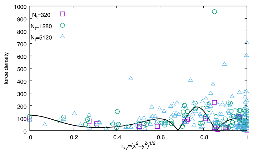
(a) Scheme A

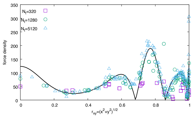
(b) Scheme B

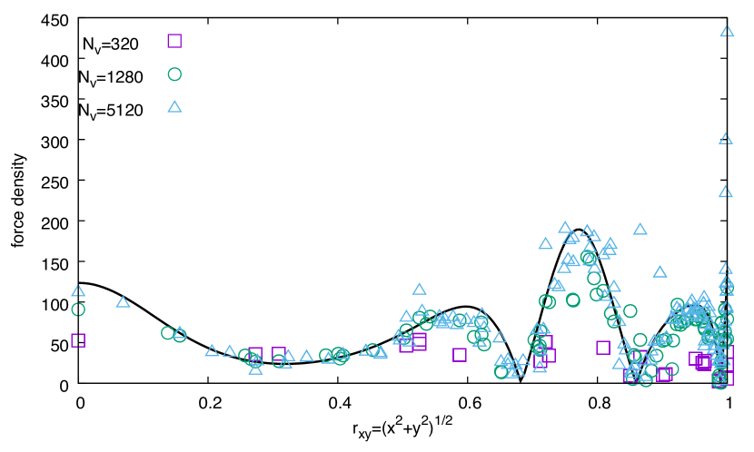
(c) Scheme C

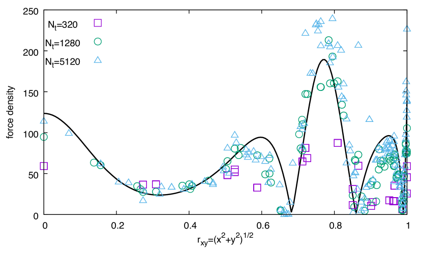
(d) Scheme D

Figure 15: Force density (absolute value) versus radial distance of vertices from axis for a biconcave oblate with $\kappa_{b}=1$, $h_{0}=0$ and $\alpha=0$. For scheme A $\tilde{\kappa}_{b}=\sqrt{3}\kappa_{b}$ and $\theta_{0}=0$.

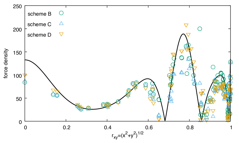
(a)

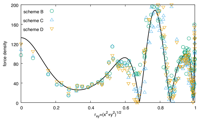
(b)

Figure 16: Force density (absolute value) versus radial distance of vertices from axis of symmetry for a biconcave oblate with $\kappa_{b}=1$, $h_{0}=-0.5$ and $\alpha=0$. (a) $N_{t}=1280$ plotted for clarity with every $4$ vertices in arbitrary order; (b) $N_{t}=5120$ and plotted for clarity with every $16$ vertices in arbitrary order.

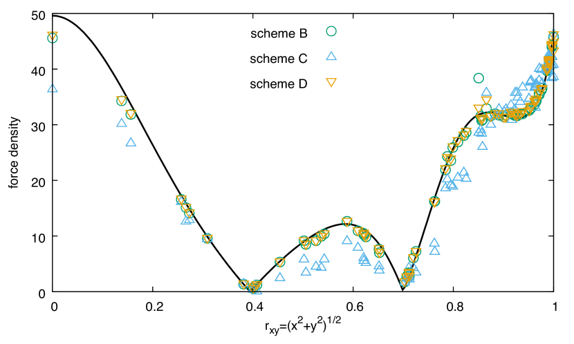
(a)

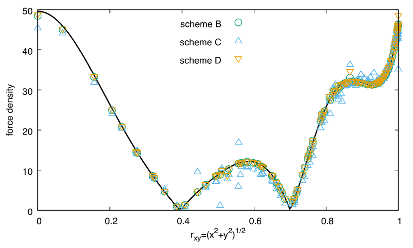
(b)

Figure 17: Force density (absolute value) versus radial distance of vertices from axis of symmetry for a biconcave oblate with $\alpha\kappa_{b}=1$. Force due to non-local ADE energy. (a) $N_{t}=1280$ plotted for clarity with every $4$ vertices in arbitrary order; (b) $N_{t}=5120$ and plotted for clarity with every $16$ vertices in arbitrary order.

For each scheme, we present the force density with three resolutions in Fig. 15, where analytical lines are computed with software Maxima. There is no convergence of force in the strict sense as reported previously. However, results from scheme B, C, D with $N_{t}\geq 1280$ follow the reference line reasonably close, with a few exceptions at turning points of the curvature. The results of scheme A are off the reference. We may draw similar conclusions from the results of Fig. 16 that all three extended schemes are noisy, but follow the reference lines closely. For the force due to ADE energy, we observe that scheme C is less accurate in comparison with the other two schemes, as show on Fig. 17.

References

References

- [1] Y. Kantor, D. R. Nelson, Phase transitions in flexible polymeric surfaces, Phys. Rev. A 36 (1987) 4020–4032.
- [2] F. Jülicher, The morphology of vesicles of higher topological genus: conformal degeneracy and conformal modes, J. Phys. II France 6 (1996) 1797–1824.
- [3] G. Gompper, D. M. Kroll, Random surface discretizations and the renormalization of the bending rigidity, J. Phys. I France 6 (1996) 1305–1320.
- [4] M. Meyer, M. Desbrun, P. Schröder, A. H. Barr, Discrete differential-geometry operators for triangulated 2-manifolds, in: H.-C. Hege, K. Polthier (Eds.), Visualization and Mathematics III, Springer Berlin Heidelberg, Berlin, Heidelberg, 2003, pp. 35–57.
- [5] H. J. Deuling, W. Helfrich, The curvature elasticity of fluid membranes: a catalogue of vesicle shapes, J. Phys. France 37 (11) (1976) 1335–1345.
- [6] U. Seifert, Configurations of fluid membranes and vesicles, Adv. Phys. 46 (1) (1997) 13–137.
- [7] M. Deserno, Fluid lipid membranes: From differential geometry to curvature stresses, Chem. Phys. Lipids 185 (2015) 11 – 45.
- [8] Z. Tu, Z.-C. Ou-Yang, J. Liu, Y. Xie, Geometric methods in elastic theory of membranes in liquid crystal phases, 2nd Edition, Vol. 2 of Peking University-World Scientific Advance Physics Series, World Scientific, 2018.
- [9] P. B. Canham, The minimum energy of bending as a possible explanation of the biconcave shape of the human red blood cell, J. Theo. Bio. 26 (1970) 61–81.
- [10] W. Helfrich, Elastic properties of lipid bilayers: theory and possible experiments, Z. Naturforsch. 28 (c) (1973) 693–703.
- [11] M. P. Sheetz, S. J. Singer, Biological membranes as bilayer couples. a molecular mechanism of drug-erythrocyte interactions, Proc. Nat. Acad. Sci. USA 71 (11) (1974) 4457–4461.
- [12] E. Evans, Bending resistance and chemically induced moments in membrane bilayers, Biophys. J. 14 (12) (1974) 923 – 931.
- [13] S. Svetina, B. Žekš, Membrane bending energy and shape determination of phospholipid vesicles and red blood cells, Euro. Biophys. J. 17 (2) (1989) 101–111.
- [14] U. Seifert, L. Miao, H.-G. Döbereiner, M. Wortis, Budding transition for bilayer fluid vesicles with area-difference elasticity, in: R. Lipowsky, D. Richter, K. Kremer (Eds.), The structure and conformation of amphiphilic membranes, Vol. 66 of Springer proceedings in physics, Springer-Verlag, 1992, pp. 93–96.
- [15] B. Boz̆ic̆, S. Svetina, B. Z̆eks̆, R. Waugh, Role of lamellar membrane structure in tether formation from bilayer vesicles, Biophys. J. 61 (4) (1992) 963 – 973.
- [16] W. Wiese, W. Harbich, W. Helfrich, Budding of lipid bilayer vesicles and flat membranes, J. Phys.: Condens. Matter 4 (7) (1992) 1647.
- [17] E. Sackmann, H.-P. Duwe, H. Engelhardt, Membrane bending elasticity and its role for shape fluctuations and shape transformations of cells and vesicles, Faraday Discuss. Soc. 81 (1986) 281–290.
- [18] J. Käs, E. Sackmann, Shape transitions and shape stability of giant phospholipid vesicles in pure water induced by area-to-volume changes, Biophy. J. 60 (4) (1991) 825 – 844.
- [19] E. A. Evans, R. Skalak, Mechanics and thermodyanics of biomembranes, CRC Press, Inc. Boca Raton, Florida, 1980.
- [20] N. Mohandas, , E. Evans, Mechanical properties of the red cell membrane in relation to molecular structure and genetic defects, Annu. Rev. Biophys. Biomol. Struct. 23 (1) (1994) 787–818.
- [21] H.-G. Döbereiner, E. Evans, M. Kraus, U. Seifert, M. Wortis, Mapping vesicle shapes into the phase diagram: A comparison of experiment and theory, Phys. Rev. E 55 (1997) 4458–4474.
- [22] A. Sakashita, N. Urakami, P. Ziherl, M. Imai, Three-dimensional analysis of lipid vesicle transformations, Soft Matter 8 (2012) 8569–8581.
- [23] A. Guckenberger, S. Gekle, Theory and algorithms to compute Helfrich bending forces: a review, J. Phys.: Condens. Matter 29 (20) (2017) 203001.
- [24] K. Crane, U. Pinkall, P. Schröder, Robust fairing via conformal curvature flow, ACM Transactions on Graphics (TOG) 32 (4) (2013) 61.
- [25] U. Seifert, K. Berndl, R. Lipowsky, Shape transformations of vesicles: Phase diagram for spontaneous- curvature and bilayer-coupling models, Phys. Rev. A 44 (1991) 1182–1202.
- [26] L. Miao, U. Seifert, M. Wortis, H.-G. Döbereiner, Budding transitions of fluid-bilayer vesicles: The effect of area-difference elasticity, Phys. Rev. E 49 (1994) 5389–5407.
- [27] V. Heinrich, S. Svetina, B. c. v. Žekš, Nonaxisymmetric vesicle shapes in a generalized bilayer-couple model and the transition between oblate and prolate axisymmetric shapes, Phys. Rev. E 48 (1993) 3112–3123.
- [28] K. Khairy, J. Foo, J. Howard, Shapes of red blood cells: comparison of 3d confocal images with the bilayer-couple model, Cell. Mol. Bioeng. 1 (2) (2008) 173.
- [29] S. K. Veerapaneni, A. Rahimian, G. Biros, D. Zorin, A fast algorithm for simulating vesicle flows in three dimensions, J. Comput. Phys. 230 (14) (2011) 5610 – 5634.
- [30] A. Yazdani, P. Bagchi, Three-dimensional numerical simulation of vesicle dynamics using a front-tracking method, Phys. Rev. E 85 (2012) 056308.
- [31] Q. Du, C. Liu, X. Wang, A phase field approach in the numerical study of the elastic bending energy for vesicle membranes, J. Comput. Phys. 198 (2) (2004) 450 – 468.
- [32] E. Maitre, T. Milcent, G.-H. Cottet, A. Raoult, Y. Usson, Applications of level set methods in computational biophysics, Mathematical and Computer Modelling 49 (11) (2009) 2161 – 2169.
- [33] M. Bergdorf, I. F. Sbalzarini, P. Koumoutsakos, A lagrangian particle method for reaction–diffusion systems on deforming surfaces, Journal of mathematical biology 61 (5) (2010) 649–663.
- [34] A. Mietke, F. Jülicher, I. F. Sbalzarini, Self-organized shape dynamics of active surfaces, Proceedings of the National Academy of Sciences 116 (1) (2019) 29–34.
- [35] H. Noguchi, G. Gompper, Shape transitions of fluid vesicles and red blood cells in capillary flows, Proc. Nat. Acad. Sci. 102 (40) (2005) 14159–14164.
- [36] I. V. Pivkin, G. E. Karniadakis, Accurate coarse-grained modeling of red blood cells, Phys. Rev. Lett. 101 (2008) 118105.
- [37] D. A. Fedosov, B. Caswell, A. S. Popel, G. E. Karniadakis, Blood flow and cell-free layer in microvessels, Microcirculation 17 (2010) 615–628.
- [38] K. Tsubota, Short note on the bending models for a membrane in capsule mechanics: comparison between continuum and discrete models, J. Comput. Phys. 277 (2014) 320 – 328.
- [39] X. Li, P. M. Vlahovska, G. E. Karniadakis, Continuum- and particle-based modeling of shapes and dynamics of red blood cells in health and disease, Soft Matter 9 (2013) 28–37.
- [40] A. Guckenberger, M. P. Schraml, P. G. Chen, M. Leonetti, S. Gekle, On the bending algorithms for soft objects in flows, Comput. Phys. Comm. 207 (2016) 1–23.
- [41] M. Jarić, U. Seifert, W. Wintz, M. Wortis, Vesicular instabilities: The prolate-to-oblate transition and other shape instabilities of fluid bilayer membranes, Phys. Rev. E 52 (1995) 6623–6634.
- [42] H. W. G. Lim, M. Wortis, R. Mukhopadhyay, Stomatocyte – discocyte – echinocyte sequence of the human red blood cell: Evidence for the bilayer – couple hypothesis from membrane mechanics, Proc. Nat. Acad. Sci. USA 99 (26) (2002) 16766–16769.
- [43] J. Barrett, H. Garcke, R. Nürnberg, Parametric approximation of Willmore flow and related geometric evolution equations, SIAM J. Sci. Comput. 31 (1) (2008) 225–253.
- [44] L. D. Landau, E. M. Lifshitz, Fluid mechanics, 2nd Edition, Volume 6 of Course of Theoretical Physics, Pergamon Press, Oxford, 1987.
- [45] R. E. Waugh, R. G. Bauserman, Physical measurements of bilayer-skeletal separation forces, Annals of Biomedical Engineering 23 (3) (1995) 308–321.
- [46] P. Ziherl, S. Svetina, Nonaxisymmetric phospholipid vesicles: Rackets, boomerangs, and starfish, Europhys. Lett. 70 (5) (2005) 690.
- [47] D. E. Discher, D. H. Boal, S. K. Boey, Simulations of the erythrocyte cytoskeleton at large deformation. ii. micropipette aspiration, Biophys. J. 75 (3) (1998) 1584 – 1597.
- [48] J. Li, M. Dao, C. Lim, S. Suresh, Spectrin-level modeling of the cytoskeleton and optical tweezers stretching of the erythrocyte, Biophys. J. 88 (5) (2005) 3707 – 3719.
- [49] G. A. Vliegenthart, G. Gompper, Compression, crumpling and collapse of spherical shells and capsules, New J. Phys. 13 (4) (2011) 045020.
- [50] T. Krüger, Computer simulation study of collective phenomena in dense suspensions of red blood cells under shear, Ph.D. thesis, Bochum University (2012).
- [51] H. S. Seung, D. R. Nelson, Defects in flexible membranes with crystalline order, Phys. Rev. A 38 (1988) 1005–1018.
- [52] F. Jülicher, Die Morphologie von Vesikeln, Ph.D. thesis, Universität zu Köln (1994).
- [53] C. Itzykson, in: J. A. et al (Ed.), Proceedings of the GIFT Seminar, Jaca 85, World Scientific, Singapore, 1986, pp. 130–188.
- [54] U. Pinkall, K. Polthier, Computing discrete minimal surfaces and their conjugates, Exp. Math. 2 (1) (1993) 15–36.
- [55] M. Hoore, F. Yaya, T. Podgorski, C. Wagner, G. Gompper, D. A. Fedosov, Effect of spectrin network elasticity on the shapes of erythrocyte doublets, Soft Matter 14 (2018) 6278–6289.
- [56] G. Thürrner, C. A. Wüthrich, Computing vertex normals from polygonal facets, J. Graphics Tools 3 (1) (1998) 43–46.
- [57] S. Jin, R. R. Lewis, D. West, A comparison of algorithms for vertex normal computation, Visual Comput. 21 (1) (2005) 71–82.
- [58] G. Boedec, M. Leonetti, M. Jaeger, 3d vesicle dynamics simulations with a linearly triangulated surface, J. Comput. Phys. 230 (4) (2011) 1020 – 1034.
- [59] K. Polthier, M. Schmies, Straightest Geodesics on Polyhedral Surfaces, Springer Berlin Heidelberg, Berlin, Heidelberg, 1998, pp. 135–150.
- [60] E. Evans, Y.-C. Fung, Improved measurement of the erythrocyte geometry, Microvasc. Res. 4 (1972) 335–347.
- [61] C. T. Loop, Smoothe subdivision surfaces based on triangles, Master’s thesis, University of Utah (1987).
- [62] P. Español, P. Warren, Statistical mechanics of dissipative particle dynamics, Europhys. Lett. 30 (4) (1995) 191–196.
- [63] K. A. Brakke, The surface evolver, Exp. Math. 1 (2) (1992) 141–165.
- [64] Z. Peng, R. J. Asaro, Q. Zhu, Multiscale simulation of erythrocyte membranes, Phys. Rev. E 81 (2010) 031904.
- [65] M. P. Do Carmo, Differential geometry of curves & surfaces, 2nd Edition, Dover Publications, Inc., New York, 2016.
- [66] A. Laadhari, C. Misbah, P. Saramito, On the equilibrium equation for a generalized biological membrane energy by using a shape optimization approach, Physica D: Nonlinear Phenomena 239 (16) (2010) 1567 – 1572.
- [67] R. Bridson, S. Marino, R. Fedkiw, Simulation of clothing with folds and wrinkles, in: ACM SIGGRAPH 2005 Courses, ACM, 2005, p. 3.
- [68] G. H. W. Lim, M. Wortis, R. Mukhopadhyay, Red blood cell shapes and shape transformations: Newtonian mechanics of a composite memebrane, Vol. 4, WILLEY-VCH Verlag GmbH & Co. KGaA, Weinheim, 2008, Ch. 2, pp. 83–249.