Effective computational methods for hybrid stochastic gene networks
Abstract
At the scale of the individual cell, protein production is a stochastic process with multiple time scales, combining quick and slow random steps with discontinuous and smooth variation. Hybrid stochastic processes, in particular piecewise-deterministic Markov processes (PDMP), are well adapted for describing such situations. PDMPs approximate the jump Markov processes traditionally used as models for stochastic chemical reaction networks. Although hybrid modelling is now well established in biology, these models remain computationally challenging. We propose several improved methods for computing time dependent multivariate probability distributions (MPD) of PDMP models of gene networks. In these models, the promoter dynamics is described by a finite state, continuous time Markov process, whereas the mRNA and protein levels follow ordinary differential equations (ODEs). The Monte-Carlo method combines direct simulation of the PDMP with analytic solutions of the ODEs. The push-forward method numerically computes the probability measure advected by the deterministic ODE flow, through the use of analytic expressions of the corresponding semigroup. Compared to earlier versions of this method, the probability of the promoter states sequence is computed beyond the naïve mean field theory and adapted for non-linear regulation functions.
Availability. The algorithms described in this paper were implemented in MATLAB. The code is available on demand.
1 Introduction
In PDMP models of gene networks, each gene promoter is described as a finite state Markov process [3, 10, 13, 12]. The promoter triggers synthesis of gene products (mRNAs and proteins) with intensities depending on its state. The promoter can exhibit two state (ON-OFF) dynamics, but also dynamics with more than two states and arbitrarily complex transitions[11, 19]. The transition rates between the states of the promoter depend on the expression levels of proteins expressed by the same or by other promoters. In PDMP models, the gene products are considered in sufficiently large copy numbers and are represented as continuous variables following ordinary differential equations (ODEs). The sources of noise in these models are thus the discrete transitions between the promoter states.
In single cell experimental settings the quantities of mRNA [18, 14, 1, 17] and proteins [5, 6] can be determined for each cell. By double or multiple- fluorophore fluorescence techniques products from several genes can be quantified simultaneously and one can have access to multivariate probability distributions (MPD) of mRNA or proteins. The stochastic dynamics of promoters and gene networks can have important consequences for fundamental biology [4] but also for HIV [15] and cancer research [7]. For this reason we aim to develop effective methods for computing time-dependent MPDs for PDMP models. Our main objective is the reduction of computation time which is prerequisite for parameter scans and machine learning applications [8].
PDMPs already represent a gain with respect to the chemical Markov equation from which they are derived by various limit theorems [2]. A gene network PDMP model can be simulated by numerical integration of ODEs coupled with a driven inhomogeneous Poisson process for the successive transitions of the promoters [20, 3, 16, 13]. The simulation becomes particularly effective when analytic solutions of the ODEs are available [10].
However, very little has been done to further improve the computational power by optimising simulation and analysis of PDMP models.
Numerical integration of the PDE satisfied by MPD is an interesting option combining precision and speed for small models. Finite difference methods, however, are of limited use in this context as they can not cope with many RNA and protein variables (extant examples are restricted to the dimension 2, corresponding to a single promoter, with or without self-regulation see [10, 12]).
Another interesting method for computing time dependent MPDs is the push-forward method. For gene networks, this method has been first introduced in [9] and further adapted for continuous mRNA variables in [10]. It is based on the idea to compute the MPD as the push-forward measure of the semigroup defined by the ODEs. This method is approximate, as one has to consider that the discrete PDMP variables are piecewise constant on a deterministic time partition. Furthermore, the transition rates between promoter states were computed in a mean field approximation. In this paper we replace the mean field approximation by the next order approximation taking into account the moments of the protein distribution.
2 Methods
2.1 PDMP models of gene networks
The state of a PDMP gene network model takes values in , where is the number of genes and is a positive integer representing the maximum number of states of a gene promoter. It is a process , determined by three characteristics:
- 1)
-
For all a vector field determining a unique global flow in , the space of all protein () and mRNA () values such that, for ,
(1) On coordinates, this reads
(2) where , , , are translation efficiencies, transcription rates, protein degradation coefficients and mRNA degradation coefficients of the gene, respectively. Note that transcription rates depend on the relevant promoter states.
The flow represents a one parameter semigroup fulfilling the properties
- (i)
-
,
- (ii)
-
.
- 2)
-
A transition rate matrix for the promoter states , such that and for all and for all .
- 3)
-
A jump rate . The jump rate can be obtained from the transition rate matrix
(3)
From these characteristics, right-continuous sample paths starting at can be constructed as follows. Define
| (4) |
where is a realisation of the first jump time of , with the distribution
| (5) |
and is the element of the probability space for which the particular realisation of the process is given. The pre-jump state is and the post-jump state is , where has the distribution
| (6) |
We then restart the process and recursively apply the same procedure at jump times , etc..
Note that between each two consecutive jumps follow deterministic ODE dynamics defined by the vector field . At the jumps, the protein and mRNA values are continuous.
The calculation of the flow between two jumps and of the jump time can be gathered in the same set of differential equations
| (7) |
that has to be integrated with the stopping condition , where is a random variable, uniformly distributed on .
We define multivariate probability density functions . These functions satisfy the Liouville-master equation which is a system of partial differential equations:
| (8) |
2.2 ON/OFF gene networks
In this paper, for the purpose of illustration only, all the examples are constituted by ON/OFF gene networks.
For an ON/OFF gene each component has two possible values for OFF and for ON.
As a first example that we denote as model , let us consider a two genes network; the expression of the first gene being constitutive and the expression of the second gene being activated by the first. We consider that the transcription activation rate of the second gene is proportional to the concentration of the first protein . All the other rates are constant , , , representing the transcription activation rate of the first gene, and the transcription inactivation rates of gene one and gene two, respectively. For simplicity, we consider that the two genes have identical protein and mRNA parameters , , . We further consider that if the gene is OFF and if the gene is ON.
The gene network has four discrete states, in order , , , and . Then, the transition rate matrix for the model is
| (9) |
The Liouville-master equation for the model reads
| (10) | |||||
The model differs from the model by the form of the activation function. Instead of a linear transcription rate we use a Michaelis-Menten model . This model is more realistic as it takes into account that the protein has to attach to specific promoter sites which become saturated when the concentration of this protein is high.
The transition rate matrix for the model is
| (11) |
The Liouville-master equation for the model reads
| (12) | |||||
2.3 Monte-Carlo method
The Monte-Carlo method utilizes the direct simulation of the PDMP based on Eq.7. A larger number of sample paths is generated and the values of are stored at selected times. Multivariate probability distributions are then estimated from this data.
The direct simulation of PDMPs needs the solutions of (7) which can be obtained by numerical integration. This is not always computationally easy. Problems may arise for fast switching promoters when the ODEs have to be integrated many times on small intervals between successive jumps. Alternatively, the numerical integration of the ODEs can be replaced by analytic solutions or quadratures. Analytic expressions are always available for the gene network flow (2) and read
| (13) |
Let us consider the following general expression of the jump intensity function
where are non-linear functions, for instance Michaelis-Menten or Hill functions . If for all , the cumulative distribution function of the waiting time can be solved analytically [10], otherwise it can be obtained by quadratures. For example, for the model one has
where is Kronecker’s delta. In this case the waiting time is obtained as the unique solution of the equation
| (14) |
where is a random variable, uniformly distributed on . In our implementation of the algorithm we solve (14) numerically, using the bisection method.
2.4 Push-forward method
This method allows one to compute the MPD of proteins and mRNAs at a time given the MPD of proteins and mRNAs at time .
In order to achieve this we use a deterministic partition of the interval such that is small. The main approximation of this method is to consider that is piecewise constant on this partition, more precisely that . This approximation is justified by Theorem 3.1 in Section 3.1.
For each path realisation of the promoter states, we can compute (see Appendix 2) the protein and mRNA levels of all genes :
| (15) | |||||
| (16) | |||||
where and if promoter is OFF for and if promoter is ON for .
In order to compute the MDP at time one has to sum the contributions of all solutions (15),(16), obtained for the realisations of promoter state paths with weights given by the probabilities of the paths.
Eqs.15,16 can straightforwardly be adapted to compute for all . To this aim, should be replaced by and should be replaced by defined by the relation .
Suppose that we want to estimate the MDP of all mRNAs and proteins of the gene network, using a multivariate histogram with bin centers where , are the numbers of bins in the protein and mRNA directions for each gene, respectively. Typically , . The initial MDP at time is given by the bin probabilities . Let be the solutions , with and . The many-to-one application provides the histogram bin in which falls the vector . The push forward MDP at time is defined by the bin probabilities that are computed as
| (17) |
In order to compute we can use the fact that, given , is a finite state Markov process, therefore
| (18) |
where is the initial distribution of the promoter state,
| (19) |
and are given by (16).
The push-forward method can be applied recursively to compute the MDP for times . The complexity of the calculation scales as which is exponential in the number of genes . The exponential complexity comes from considering all the possible paths . However, many of these paths have almost the same probability and impose very similar trajectories to the variables . In fact, a convenient approximation is to consider that different genes are switching between ON and OFF states according to Markov processes with rates given by the mean values of regulatory proteins (mean field approximation, [10]). This approximation consists in applying the push-forward procedure for each gene separately, using averaged transition probabilities. Thus, the states transition matrix has to be replaced by , state transition matrices for each gene. This approximation reduces the complexity of the calculations to which is linear in the number of genes.
In [10] we have replaced the regulation term occurring in the transition matrix by its mean . In this case both and can be computed analytically, which leads to a drastic reduction in the execution time. This approach is suitable for the model , which contains only linear regulation terms. For non-linear regulation terms, can not generally be computed analytically. Furthermore, the mean field approximation introduces biases. For instance, in the case of the model , the approximation is poor. A better approximation in this case is to replace by its mean and use
| (20) |
in order to correct the bias. Here indicates the variance.
As in [10] we can use analytic expressions for , but also for . These expressions can be found in Appendix 1. Although the elements of matrix have analytic expressions, the elements of the matrix contain integrals that must be computed numerically. For the model , we have
| (21) |
for the transition rates of the first gene, where , , and
| (22) | ||||
for the transitions of the second gene, where .
3 Results
3.1 Convergence of the push-forward method
The probability distribution obtained with the push-forward method converges to the exact PDMP distribution in the limit . This is a consequence of the following theorem
Theorem 3.1
Let be the flow defined by the formulas (16),(15), such that for , and let be the probability measure defined as , where is the probability distribution of at , are given by (18), and are the Borel sets on . Let , the exact distribution of for the PDMP defined by (1),(2),(3), with initial values distributed according to . Assume that for all , where is a positive constant. Then, for all , converges in distribution to , when .
The proof of this theorem is given in the Appendix 3.
3.2 Testing the push-forward method
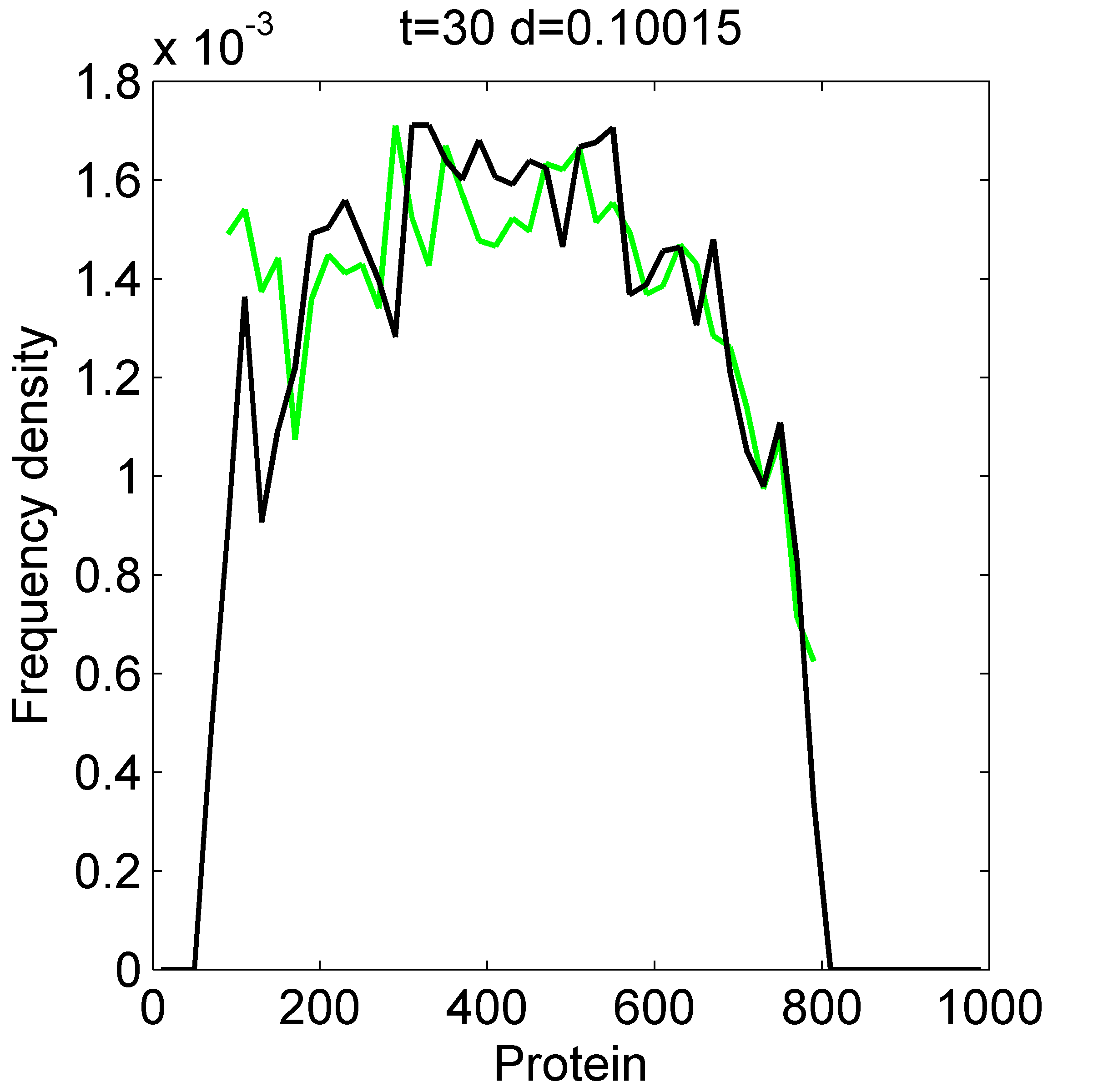
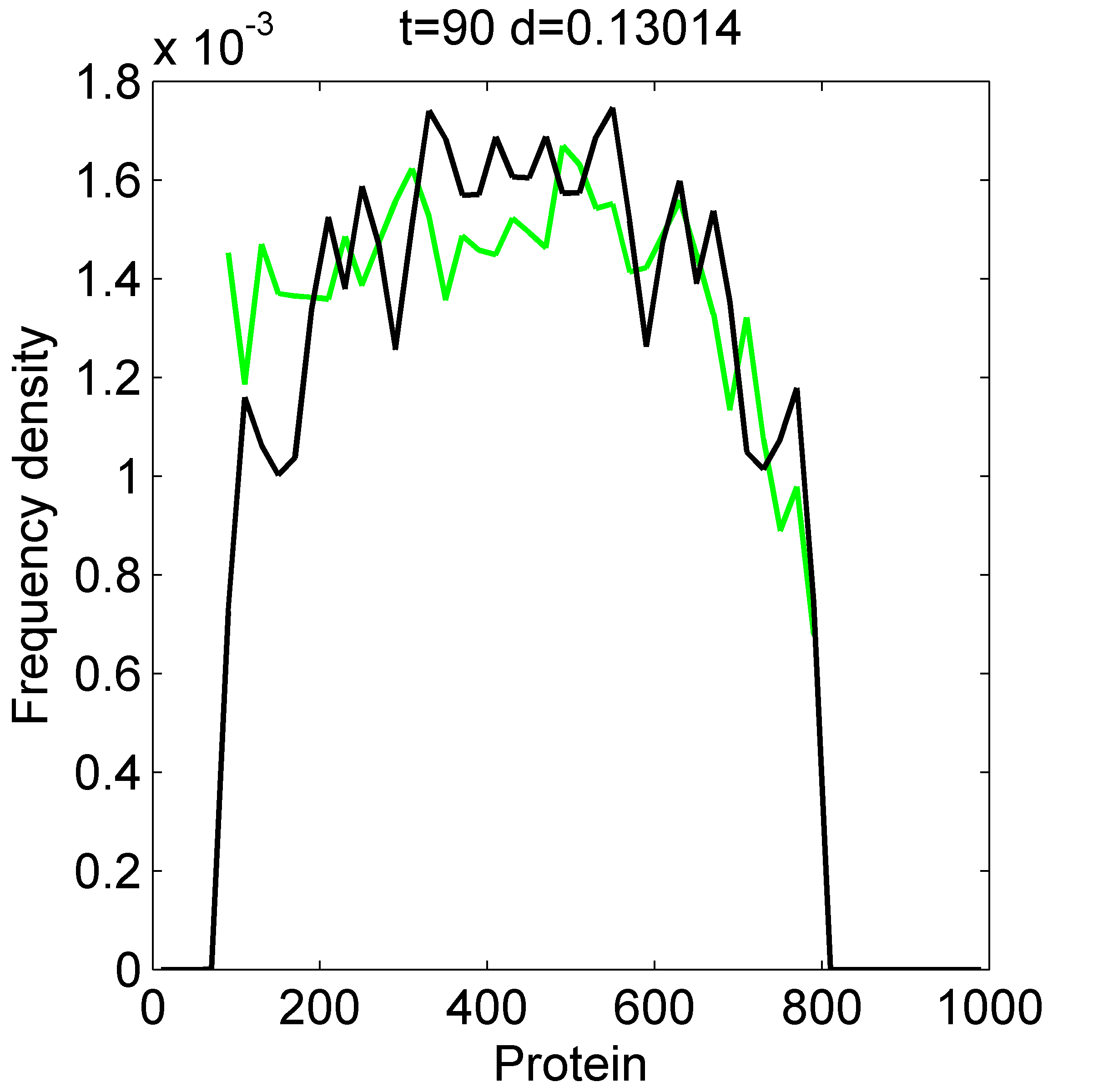
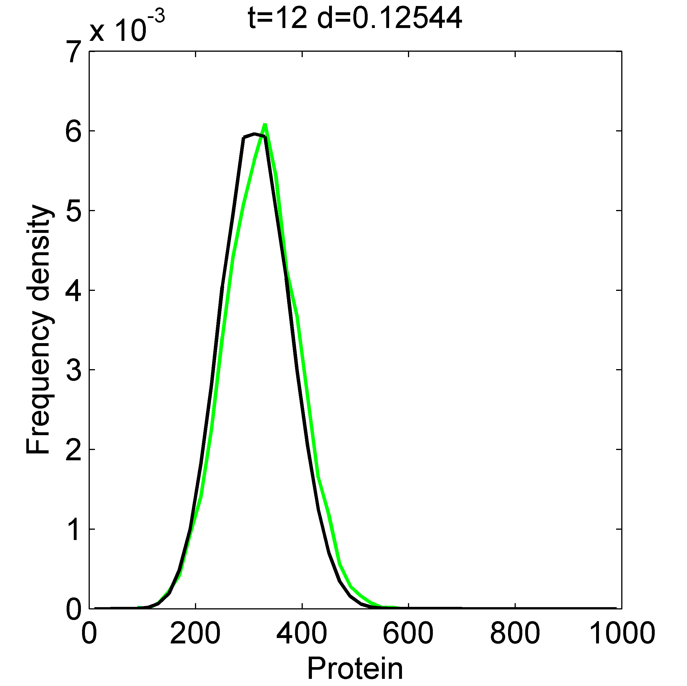
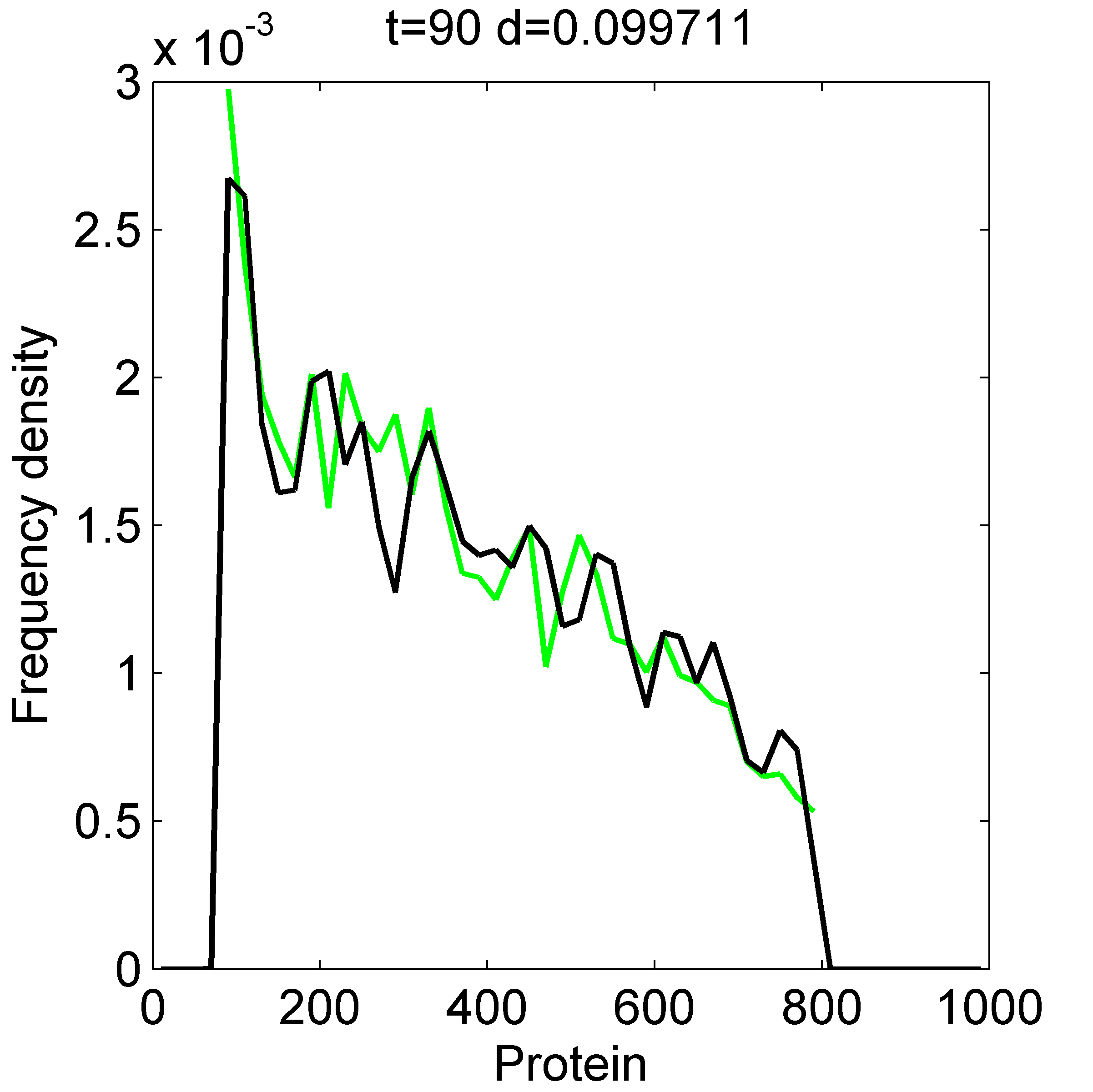
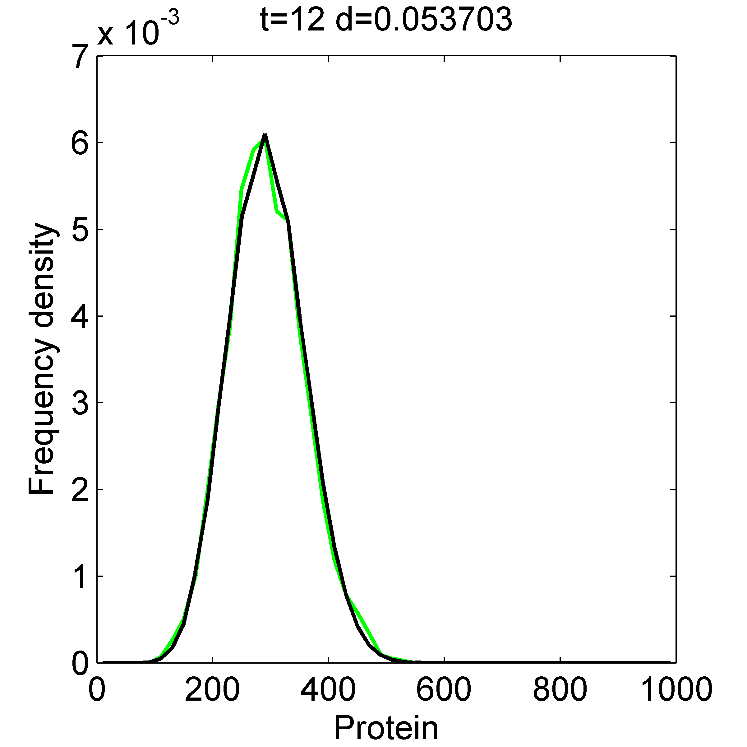
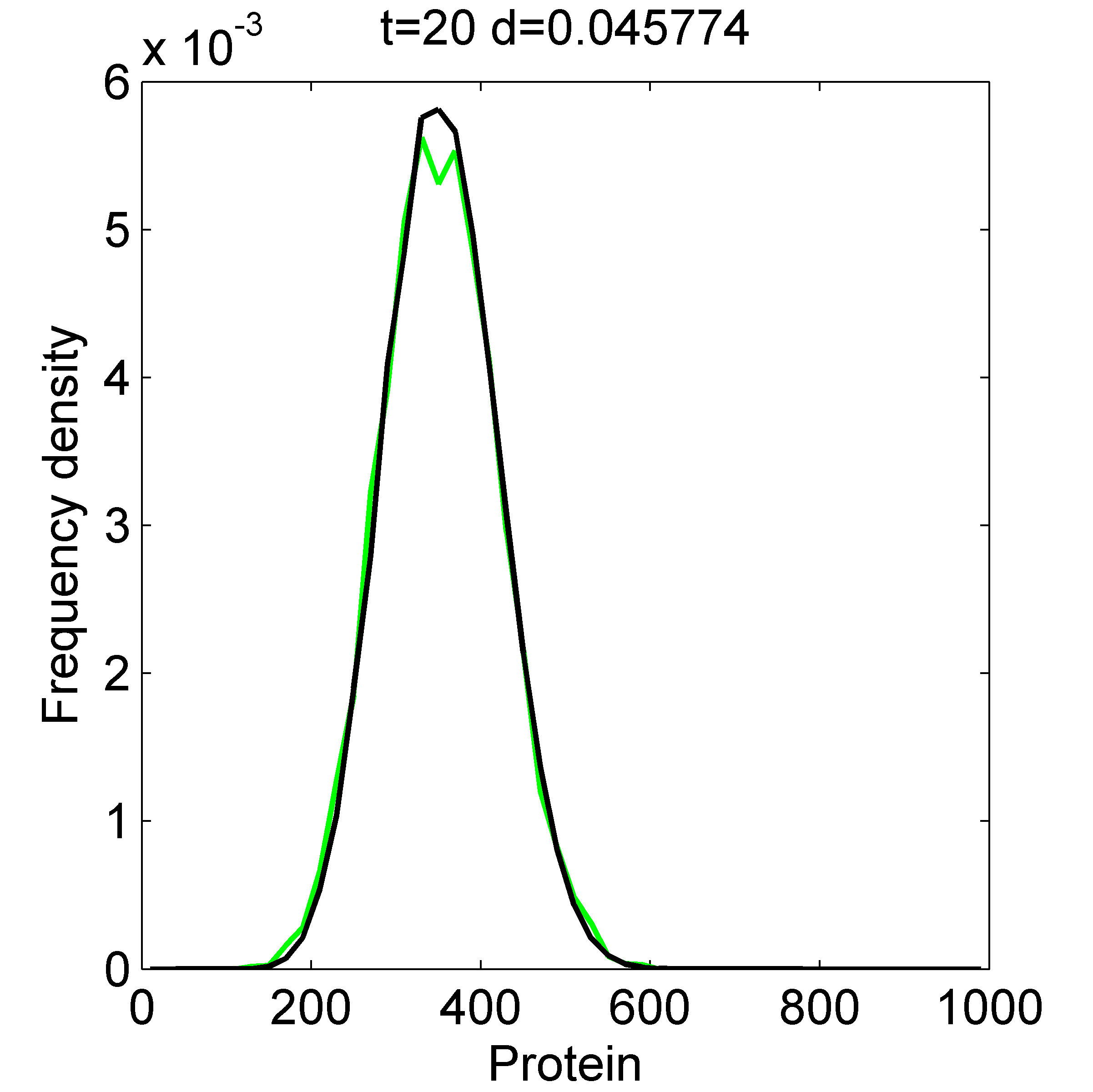
In order to test the push-forward method, we compared the resulting probability distributions with the ones obtained by the Monte Carlo method using the direct simulation of the PDMP. We considered the models and with the following parameters: , , , , , for the two genes. The parameter took two values for slow genes and for fast genes. We tested the slow-slow and the fast-fast combinations of parameters.
The initial distribution of the promoters states was where the state means that both promoters are OFF. The initial probability measure was a delta Dirac distribution centered at and . This is obtained by always starting the direct simulation of the PDMP from , , and . The simulations were performed between and for fast genes and between and for slow genes. In order to estimate the distributions we have used samples.
The push-forward method was implemented with equal length sub-intervals of . The time step was chosen for fast genes and for slow genes. The procedure was iterated times for fast genes (up to ) and times for slow genes (up to ).
The execution times are provided in the Table 1. The comparison of the probability distributions are illustrated in the Figures 1,2. In order to quantify the relative difference between methods we use the distance between distributions. More precisely, if and are probability density functions to be compared, the distance between distributions is
| (23) |
| Model | Monte-Carlo [min] | Push-forward [s] |
|---|---|---|
| slow-slow | 45 | 20 |
| fast-fast | 74 | 30 |
| slow-slow | 447 | 20 |
| fast-fast | 758 | 30 |


4 Discussion and conclusion
Combining direct simulation of PDMP gene network models and analytic formulas for the ODE flow represents an effective, easy to implement method for computing time dependent MPD of these models. However, the precision of the Monte-Carlo estimates of the distributions increases like , where is the number of Monte-Carlo samples. For this reason, the execution time of this method, although smaller compared to PDMP simulation methods that implement numerical resolution of the ODEs such as reported in [13] (data not shown), is large compared to deterministic methods such as the push-forward method.
The push-forward method represents an effective alternative to Monte-Carlo methods, ensuring reduced execution time. With respect to an earlier implementation of this method in [9] we used promoter states instead of mRNA copy numbers as discrete variables of the PDMP. As a consequence, the number of discrete states is lower and we can afford increasing the number of time subdivisions. Compared to the similar work in [10] we used second moments of the protein distribution which took into account the correlation of the promoter states and lead to increased accuracy in the case of nonlinear regulation. We proved rigorously the convergence of the distributions calculated with the push-forward method to the exact distributions of the PDMP. However, the push-forward method is an approximate method, and its accuracy relies on the careful choice of the time and space steps, namely of the integers , , , . We will present elsewhere error estimates allowing an optimal choice of these parameters. Although the protein moments and the exponential transition rate matrix can be computed numerically, the effectiveness of the push-forward method is increased when analytic expressions are available for these quantities. In this paper, these expressions were computed for particular cases. In the future, we will provide expressions, as well as symbolic computation tools to compute these quantities in more general cases. We situate our findings in the broader effort of the community to produce new effective tools for computational biology by combining numerical and symbolic methods.
Appendix1: mean and variance of the protein
We compute here the mean and the variance of the protein synthesized by a constitutive promoter (gene 1 of models and ).
We start with
| (24) |
where if the promoter is OFF and if the promoter is ON at the time .
Eq.24 leads to
| (25) |
From (25) it follows
| (26) |
The promoter state variable follows the master equation
| (27) |
that has the solution
| (28) |
where , , and . Using straightforward algebra, we find
| (29) |
where
| (30) | |||||
| (31) | |||||
| (32) | |||||
| (33) |
From (25) we find also
| (34) |
We have considered here that , are uncorrelated, but more general expressions can be obtained.
In order to compute the two times covariance we combine the tower property of the conditional expectation with the Markov property satisfied by . More precisely, for we find and . Then, it follows
| (35) |
is a Bernoulli variable, therefore . From (35) and (28) it follows
| (36) |
Similarly, one gets
| (37) |
The domain of the multiple integral in (34) should be split in two sub-domains corresponding to and to . Each of these sub-domains should be subdivided into two smaller sub-domains corresponding to and . Symmetry arguments imply that the integrals on and on are equal, which allows us to perform the calculation of the integral on only two sub-domains, instead of four. After some algebra we find
| (38) |
where
| (39) |
Appendix2: details of the derivation of (15),(16)
and satisfy the following system of equations
| (40) |
For simplification, we rescale variables and parameters , , , and obtain
| (41) |
From (41) we also obtain where
In order to compute the integral we decompose the triangular integration domain into rectangles and triangles on each of which is constant, as in Figure3.
The contribution of each rectangle to the integral is .
The contribution of each triangle to the integral is .
It follows that
Noting that the first sum in the expression of can go to (the M-th term is zero) we obtain (16).

Appendix3: proof of the Theorem 3.1
The proof the Theorem 1 relies on the following Lemma:
Lemma 4.1
We prove this Lemma for . The proof for follows the same principles.
According to the constructive definitions of PDMP (see Section 2.1), and considering that , for all (this follows from the continuity of and the boundedness of , and ) then, with probability one, has a finite number of jumps inside the interval . Consider that for the gene there are jumps such that changes from ON to OFF or from OFF to ON. The positions of these jumps are , for . Using (15) it follows .
For constitutive promoters the number of jumps of the promoter of the gene inside has a mean . Slightly more complex, but finite bounds, can be obtained for a regulated gene as well.
Using Markov’s inequality we find that . It follows that when , for any .
The proof of the Theorem 1 follows from the Lemma 4.1 because by construction, the promoter states have the same distribution in the push-forward and PDMP schemes, and the convergence in probability of the mRNAs and of the proteins implies the convergence in distribution of these variables.
References
- [1] Long Cai, Nir Friedman, and X Sunney Xie. Stochastic protein expression in individual cells at the single molecule level. Nature, 440(7082):358, 2006.
- [2] A. Crudu, A. Debussche, A. Muller, and O. Radulescu. Convergence of stochastic gene networks to hybrid piecewise deterministic processes. Annals of Applied Probability, 22:1822–1859, 2012.
- [3] A. Crudu, A. Debussche, and O. Radulescu. Hybrid stochastic simplifications for multiscale gene networks. BMC Systems Biology, 3(1):89, 2009.
- [4] Avigdor Eldar and Michael B Elowitz. Functional roles for noise in genetic circuits. Nature, 467(7312):167, 2010.
- [5] Michael B Elowitz, Arnold J Levine, Eric D Siggia, and Peter S Swain. Stochastic gene expression in a single cell. Science, 297(5584):1183–1186, 2002.
- [6] M.L Ferguson,D. Le Coq,M. Jules,S. Aymerich,O. Radulescu,N. Declerck, and C.A. Royer. Reconciling molecular regulatory mechanisms with noise patterns of bacterial metabolic promoters in induced and repressed states. Proceedings of the National Academy of Sciences USA, 109:155, 2012.
- [7] Piyush B Gupta, Christine M Fillmore, Guozhi Jiang, Sagi D Shapira, Kai Tao, Charlotte Kuperwasser, and Eric S Lander. Stochastic state transitions give rise to phenotypic equilibrium in populations of cancer cells. Cell, 146(4):633–644, 2011.
- [8] Ulysse Herbach, Arnaud Bonnaffoux, Thibault Espinasse, and Olivier Gandrillon. Inferring gene regulatory networks from single-cell data: a mechanistic approach. BMC systems biology, 11(1):105, 2017.
- [9] Guilherme CP Innocentini, Michael Forger, Ovidiu Radulescu, and Fernando Antoneli. Protein synthesis driven by dynamical stochastic transcription. Bulletin of mathematical biology, 78(1):110–131, 2016.
- [10] Guilherme CP Innocentini, Arran Hodgkinson, and Ovidiu Radulescu. Time dependent stochastic mrna and protein synthesis in piecewise-deterministic models of gene networks. Frontiers in Physics, 6:46, 2018.
- [11] Guilherme da Costa Pereira Innocentini, Michael Forger, Alexandre Ferreira Ramos, Ovidiu Radulescu, and José Eduardo Martinho Hornos. Multimodality and flexibility of stochastic gene expression. Bulletin of mathematical biology, 75(12):2600–2630, 2013.
- [12] Pavel Kurasov, Alexander Lück, Delio Mugnolo, and Verena Wolf. Stochastic hybrid models of gene regulatory networks–a pde approach. Mathematical biosciences, 305:170–177, 2018.
- [13] Yen Ting Lin and Nicolas E Buchler. Efficient analysis of stochastic gene dynamics in the non-adiabatic regime using piecewise deterministic markov processes. Journal of The Royal Society Interface, 15(138):20170804, 2018.
- [14] Arjun Raj, Charles S Peskin, Daniel Tranchina, Diana Y Vargas, and Sanjay Tyagi. Stochastic mrna synthesis in mammalian cells. PLoS biology, 4(10):e309, 2006.
- [15] Brandon S Razooky, Anand Pai, Katherine Aull, Igor M Rouzine, and Leor S Weinberger. A hardwired hiv latency program. Cell, 160(5):990–1001, 2015.
- [16] Martin G Riedler. Almost sure convergence of numerical approximations for piecewise deterministic markov processes. Journal of Computational and Applied Mathematics, 239:50–71, 2013.
- [17] Katjana Tantale, Florian Mueller, Alja Kozulic-Pirher, Annick Lesne, Jean-Marc Victor, Marie-Cécile Robert, Serena Capozi, Racha Chouaib, Volker Bäcker, Julio Mateos-Langerak, et al. A single-molecule view of transcription reveals convoys of rna polymerases and multi-scale bursting. Nature communications, 7:12248, 2016.
- [18] Mukund Thattai and Alexander Van Oudenaarden. Stochastic gene expression in fluctuating environments. Genetics, 167(1):523–530, 2004.
- [19] Philipp Thomas, Nikola Popović, and Ramon Grima. Phenotypic switching in gene regulatory networks. Proceedings of the National Academy of Sciences, 111(19):6994–6999, 2014.
- [20] Stefan Zeiser, Uwe Franz, Olaf Wittich, and Volkmar Liebscher. Simulation of genetic networks modelled by piecewise deterministic markov processes. IET systems biology, 2(3):113–135, 2008.