Generalized diffusion-wave equation with memory kernel

Abstract

We study generalized diffusion-wave equation in which the second order time derivative is replaced by integro-differential operator. It yields time fractional and distributed order time fractional diffusion-wave equations as particular cases. We consider different memory kernels of the integro-differential operator, derive corresponding fundamental solutions, specify the conditions of their non-negativity and calculate mean squared displacement for all cases. In particular, we introduce and study generalized diffusion-wave equations with regularized Prabhakar derivative of single and distributed orders. The equations considered can be used for modeling broad spectrum of anomalous diffusion processes and various transitions between different diffusion regimes.

1 Introduction

Diffusion equations with fractional time and space derivatives instead of the integer ones are widely used to describe anomalous diffusion processes where the mean squared displacement (MSD) scales as a power of time,

$$\left\langle x^{2}(t)\right\rangle\simeq t^{\alpha},$$ (1)

where $\alpha\neq 1$ [44]. If $0<\alpha<1$, the process is subdiffusive, if $1<\alpha<2$ the process is superdiffusive. Ballistic diffusion corresponds to $\alpha=2$, whereas $\alpha>2$ corresponds to superballlistic motion. At $\alpha=1$ one has normal Brownian diffusion that obeys the usual diffusion equation with the time and space derivatives of the first and second orders, respectively. Classical examples of subdiffusion include charge carrier motion in semiconductors [60], spreading of tracer chemicals in subsurface aquifers [5], as well as the motion of passive particles in atmospheric convection rolls [67]. Superdiffusion is known from tracer motion in chaotic laminar flows, which takes place due to vortices working as traps [64], plasma turbulence in fusion devices [14], diffusion in porous structurally inhomogeneous media [71], or from random search, like actively moving bacteria [1] and animals [68], or from human travels [6].

Modern microscopic techniques such as fluorescence correlation spectroscopy or advanced single particle tracking methods have led to the discovery of a multitude of anomalous diffusion processes in living biological cells and complex fluids, see e.g., the reviews [2, 26, 42, 45, 48, 59] and references therein. With the number of anomalous diffusion phenomena growing it became clear that most of the complex systems do not show a mono-scaling behavior, Eq.(1), but instead demonstrate transitions between different diffusion regimes in course of time. Such observations put forward the idea that in order to capture such multi-scaling situations one could replace relatively simple operators of fractional derivatives by more general operators with specific memory kernels. Then, a special case of a power-law kernel recovers fractional derivative and respectively, the mono-scaling diffusion regime. Thus, the distributed order fractional diffusion equations in the normal and modified forms have been suggested in order to describe the processes which become more anomalous (retarding subdiffusion or accelerating superdiffusion) or less anomalous (accelerating subdiffusion and decelerating superdiffusion) in course of time [9, 10, 11, 12, 13, 63]. The solutions of such distributed order equations have been obtained, and the relation to continuous time random walk models has been investigated in detail [22, 24, 34, 35, 53, 55, 56]. Other forms of kernels contain for example, distributed, tempered, distributed tempered and Mittag-Leffler memory functions [13, 27, 53, 55, 57, 65], to name but a few.

In analogy to the generalized diffusion equation with memory kernel introduced in [53] (see also [57]), here we introduce the following generalized diffusion-wave equation

$$\int_{0}^{t}\eta(t-t^{\prime})\frac{\partial^{2}}{\partial t^{\prime 2}}W(x,t)\,dt^{\prime}=\frac{\partial^{2}}{\partial x^{2}}W(x,t),$$ (2)

with non-negative memory kernel $\eta(t)$ of physical dimension $[\eta(t)]=\mathrm{m}^{-2}\mathrm{s}^{1}$, where $W(x,t)$ is the field variable. In what follows for simplicity we use dimensionless units. Here we note that $W(x,t)$ could be either a probability distribution function (PDF) of particles which should be non-negative, or electric field or velocity, where the non-negativity might not be needed. In Ref. [53] a similar equation – called generalized diffusion equation – was suggested, that contains a first order time derivative in the integrand, and the corresponding continuous time random walk model was also developed. Different generic forms of the memory kernel have been employed (power-law, truncated power-law, Mittag-Leffler and truncated Mittag-Leffler) in order to demonstrate the variety of anomalous diffusion regimes that could be described within the suggested generalized diffusion equation. The present paper can be considered as a natural continuation and extension of such kind of research aiming to give a comprehensive description of anomalous diffusion phenomena. In what follows we thus consider $W(x,t)$ as a PDF and study solutions of Eq. (2) in the infinite domain with zero boundary conditions at infinity, $W(\pm\infty,t)=0$, $\frac{\partial}{\partial x}W(\pm\infty,t)=0$. We take the initial conditions of the form

$$W(x,t=0)=\delta(x),\quad\frac{\partial}{\partial t}W(x,t=0)=0.$$ (3)

The first initial condition is obvious since it corresponds to the particle initially starting at $x=0$. This is a standard set-up used in the papers on anomalous diffusion processes where the mean square displacement is calculated as a function of time in the infinite space domain. Second initial condition must be imposed on $\frac{\partial}{\partial t}W(x,t)$ because of the second time derivative that appears in the generalized diffusion wave equation (2) in the integrand of the left hand side. To the authors opinion the concretization of such condition is not a trivial task. Similar problem appeared for telegrapher’s equation [36, 69] and its fractional generalizations reproducing anomalous diffusion laws [15, 43, 46]. In Refs. [36, 69] the zero second initial condition was derived from the underlining random walk scheme under the specific assumption that the initial tendency to move in one direction or another is non-biased. In Refs. [15, 43, 46] the zero second initial condition was also employed implicitly without addressing to the corresponding continuous time random walk model. To the authors knowledge at present time a stochastic approach to the generalized diffusion-wave equation (2) is lacking (note that instead, for the generalized diffusion equation such approach was recently developed in Refs. [53, 55]). Under these circumstances, in what follows we pay main attention to the particular case of the zero second initial condition, Eq. (3). However, in Section 4 we provide discussion of how the anomalous diffusion regimes found in the paper can be modified in presence of non-zero second initial condition, and which restrictions on such initial condition must be imposed. We note that for the special case of the memory kernel

$$\eta(t)=\int_{1}^{2}p(\lambda)\frac{t^{1-\lambda}}{\Gamma(2-\lambda)}\,d\lambda,$$

where the weight function $p(\lambda)$ satisfies $\int_{1}^{2}p(\lambda)\,d\lambda=1$, one recovers the distributed order wave equation considered by Gorenflo, Luchko and Stojanovic [23], i.e.,

$$\int_{1}^{2}p(\lambda)\,{{}_{C}D_{t}^{\lambda}}W(x,t)\,d\lambda=\frac{\partial^{2}}{\partial x^{2}}W(x,t),\quad 1<\lambda<2,$$ (4)

where ${{}_{C}D_{t}^{\lambda}}$ is the Caputo fractional derivative of order $\lambda$ [50]

$${{}_{C}D_{t}^{\lambda}}f(t)=\frac{1}{\Gamma(n-\lambda)}\int_{0}^{t}(t-t^{\prime})^{n-1-\lambda}\frac{d^{n}}{dt^{\prime n}}f(t^{\prime})\,dt^{\prime},$$ (5)

$n-1<\lambda<n$, $n\in N$. The case with $p(\lambda)=\delta(\lambda-\mu)$ recovers fractional diffusion-wave equation which was studied in different contexts in [23, 40, 41, 32, 31, 3, 4, 62]. In [23] the authors derived the fundamental solutions of Eq. (4) for different forms of the weight function, and discussed the non-negativity of the solution by using the properties of completely monotone, Bernstein and Stieltjes functions. In this paper we introduce other generalized memory kernels and analyse properties of the solutions.

The paper is organized as follows. In Section 2 we derive the solution of the generalized diffusion-wave equation (2). We find the constraints on the memory kernel, which guarantee non-negativity of the solution. We give general formula for the moments of the fundamental solution. Special cases of the memory kernel are considered in Section 3, and the corresponding solutions and second moments are obtained. In Section 4 we discuss the role of a second non-zero initial condition. The summary is given in Section 5.

2 General solution and its fractional moments

2.1 Completely monotone and Bernstein functions

Before finding fundamental solution of the model proposed we recall definitions and some properties of the completely monotone (CM) and Bernstein functions (BF) [61], which are used to show the non-negativity of the fundamental solution.

2.1.1 Completely monotone functions.

Completely monotone function $\mathcal{M}(s)$ is defined in non-negative semi-axis and have a property that

$$(-1)^{n}\mathcal{M}^{(n)}(s)\geq 0\quad\textrm{for all $n\in\mathrm{N}_{0}$ and $s\geq 0$}.$$ (6)

According to the famous Bernstein theorem the completely monotone function can be represented as a Laplace transform of non-negative function $p(t)$ (see, for example, Chapter XIII, Section 4 in Ref. [16]), i.e.,

$$\mathcal{M}(s)=\int_{0}^{\infty}p(t)e^{-st}\,dt.$$ (7)

The following properties hold true for CM functions:

• Linear combination $a_{1}\mathcal{M}_{1}(s)+a_{2}\mathcal{M}_{2}(s)$ ($a_{1},a_{2}\geq 0$) of completely monotone functions $\mathcal{M}_{1}(s)$ and $\mathcal{M}_{2}(s)$ is completely monotone function as well;

• The product $\mathcal{M}(s)=\mathcal{M}_{1}(s)\mathcal{M}_{2}(s)$ of completely monotone functions $\mathcal{M}_{1}(s)$ and $\mathcal{M}_{2}(s)$ is again completely monotone function.

An example of completely monotone function is $s^{\alpha}$, where $\alpha\leq 0$.

2.1.2 Stieltjes functions.

A function defined in the non-negative semi-axis, which is Laplace transform of CM function is called Stieltjes function (SF). The Stieltjes functions are a subclass of the completely monotone functions. For the SFs the following property holds true:

• Linear combination $a_{1}\mathcal{S}_{1}(s)+a_{2}\mathcal{S}_{2}(s)$ ($a_{1},a_{2}\geq 0$) of SFs $\mathcal{S}_{1}(s)$ and $\mathcal{S}_{2}(s)$ is SF;

An example of SF is $s^{\alpha-1}$, where $0\leq\alpha\leq 1$.

2.1.3 Bernstein functions.

The Bernstein function is a non-negative function whose derivative is completely monotone, that is

$$(-1)^{(n-1)}\mathcal{B}^{(n)}(s)\geq 0\quad\textrm{for all $n=1,2,\dots$}$$

BFs have the following properties:

• Linear combination $a_{1}\mathcal{B}_{1}(s)+a_{2}\mathcal{B}_{2}(s)$ ($a_{1},a_{2}\geq 0$) of BFs $\mathcal{B}_{1}(s)$ and $\mathcal{B}_{2}(s)$ is a BF;

• A composition $\mathcal{M}(\mathcal{B}(s))$ of CM function $\mathcal{M}(s)$ and BF $\mathcal{B}(s)$ is CM function.

From these properties it follows that the function $e^{-u\,\mathcal{B}(s)}$ is CM for $u>0$ if $\mathcal{B}(s)$ is a BF.

An example of a BF is $s^{\alpha}$, where $0\leq\alpha\leq 1$.

2.1.4 Complete Bernstein functions.

The complete Bernstein functions (CBFs) are subclass of BFs. A function $\mathcal{C}(s)$ on $(0,\infty)$ is a CBF if and only if $\mathcal{C}(s)/s$ is a SF.

The following properties are valid for the complete Bernstein functions:

• A composition $\mathcal{S}(\mathcal{C}(s))$ of SF $\mathcal{S}(s)$ and CBF $\mathcal{C}(s)$ is a SF;

• A composition $\mathcal{C}(\mathcal{S}(s))$ of CBF $\mathcal{C}(s)$ and SF $\mathcal{S}(s)$ is SF;

• If $\mathcal{C}(s)$ is a CBF, then $\mathcal{C}(s)/s$ is SF.

An example of complete Bernstein function is $s^{\alpha}$, where $0<\alpha<1$.

2.2 Fundamental solution

At first let us consider the generalized diffusion-wave equation (2) with the memory kernel $\eta(t)$ of a general form. The restrictions on the memory kernel are discussed below. In order to find the solution of equation (2) we use the Fourier $(\tilde{F}(\kappa)=\int_{-\infty}^{\infty}f(x)e^{\imath\kappa x}\,dx)$ and Laplace $(\hat{f}(s)=\int_{0}^{\infty}f(t)e^{-st}\,dt)$ transformations. For initial conditions $W(x,0)=\delta(x)$ and $\frac{\partial}{\partial t}W(x,0)=0$, and zero boundary conditions we find

$$\tilde{\hat{W}}(\kappa,s)=\frac{s\hat{\eta}(s)}{s^{2}\hat{\eta}(s)+\kappa^{2}}.$$ (8)

By the inverse Fourier transformation of Eq. (8) we find the PDF in the Laplace space

$$\hat{W}(x,s)=\frac{1}{2}\sqrt{\hat{\eta}(s)}\exp\left(-s\sqrt{\hat{\eta}(s)}|x|\right),$$ (9)

from which one can find either the exact form of $W(x,t)$ or (at least) its asymptotic behavior by using Tauberian theorems [16]. From Eq. (9) one can easily conclude that the PDF is normalized to 1, i.e., $\int_{-\infty}^{\infty}W(x,t)\,dx=1$, since $\int_{-\infty}^{\infty}\hat{W}(x,s)\,dx=\frac{1}{s}$.

The non-negativity of the solution of the distributed order wave equation has been shown in [23] by using the properties of CM functions and BFs. In order to find the constraints for the memory kernel $\eta(t)$ under which the considered generalized diffusion-wave equation (2) has a non-negative solution we use representation (9) in the Laplace space together with relation (7). The solution (9) can be considered as a product of two functions, $\frac{1}{2}\sqrt{\hat{\eta}(s)}$ and $\exp\left(-s\sqrt{\hat{\eta}(s)}|x|\right)$. In order to show non-negativity of the PDF $W(x,t)$ one should prove that its Laplace transform $\hat{W}(x,s)$ is a CM function. Thus, it is sufficient to prove that both functions

$$\sqrt{\hat{\eta}(s)}\quad\mathrm{and}\quad\exp\left(-s\sqrt{\hat{\eta}(s)}|x|\right)$$

are CM (see property (b) in Section 2.1.1.). Therefore, it is sufficient to show that $\sqrt{\hat{\eta}(s)}$ is CM function, and $s\sqrt{\hat{\eta}(s)}$ is BF, according to the property (e) in Section 2.1.3. The non-negativity of the solution can also be shown by proving that the function $\sqrt{\hat{\eta}(s)}$ is SF, which is again a CM function, or that $s\sqrt{\hat{\eta}(s)}$ is CBF, which follows from the properties (f) and (g) in Section 2.1.4.

Remark 1. Here we note that the subordination approach, which was used to prove the non-negativity of the PDF in case of fractional and distributed order diffusion equations [23, 53], can not be applied in case of generalized diffusion-wave equations. Indeed, the solution (8) can be rewritten in a form of subordination integral as

$$\tilde{\hat{W}}(k,s)=s\hat{\eta}(s)\int_{0}^{\infty}e^{-u[s^{2}\hat{\eta}(s)+k^{2}]}\,du=\int_{0}^{\infty}e^{-uk^{2}}\hat{G}(u,s)\,du,$$ (10)

where

$$\hat{G}(u,s)=s\hat{\eta}(s)e^{-us^{2}\hat{\eta}(s)}.$$

Therefore, the PDF $W(x,t)$ becomes

$$W(x,t)=\int_{0}^{\infty}\frac{e^{-\frac{x^{2}}{4u}}}{\sqrt{4\pi u}}G(u,t)\,du.$$ (11)

From here it follows that in order $W(x,t)$ to be non-negative, the function $G(u,t)$ should be non-negative, that is $\hat{G}(u,s)$ should be CM. For this it is sufficient to show that $s\hat{\eta}(s)$ is CM and $s^{2}\hat{\eta}(s)$ is a BF according to property $(\textrm{{\bf e}})$ in Section 2.1.3. Such approach works well in case of fractional and distributed order diffusion equations but, as we will see later, not in case of generalized diffusion-wave equation. This was already noted in [23] while proving the non-negativity of the distributed order diffusion-wave equation that is a particular case of the generalized diffusion-wave equation.

2.3 Fractional moments

From Eq. (8) we calculate the $q$-th moment $\left\langle|x|^{q}(t)\right\rangle=\int_{-\infty}^{\infty}|x|^{q}W(x,t)\,dx=2\int_{0}^{\infty}x^{q}W(x,t)\,dx$ of the solution of Eq. (2), which is given by

$$\left\langle|x|^{q}(t)\right\rangle=\Gamma(q+1)\mathcal{L}^{-1}\left[\frac{s^{-1}}{\left(s^{2}\hat{\eta}(s)\right)^{q/2}}\right](t).$$ (12)

For the second moment we find

$$\left\langle x^{2}(t)\right\rangle=\left.\left\{-\frac{\partial^{2}}{\partial\kappa^{2}}\mathcal{L}^{-1}\left[\tilde{\hat{W}}(\kappa,s)\right](\kappa,t)\right\}\right|_{\kappa=0}=2\,\mathcal{L}^{-1}\left[\frac{1}{s^{3}\hat{\eta}(s)}\right](t),$$ (13)

from where one can analyze diffusion regimes for different forms of the memory function $\eta(t)$.

3 Special cases

In this Section we analyze solutions of the generalized diffusion-wave equation for different forms of the memory kernel. We also calculate the mean squared displacement for each of the cases.

3.1 Standard wave equation. Dirac delta memory kernel

Eq. (4) for a Dirac delta memory kernel $\eta(t)=\delta(t)$ yields the classical wave equation

$$\frac{\partial^{2}}{\partial t^{2}}W(x,t)=\frac{\partial^{2}}{\partial x^{2}}W(x,t).$$ (14)

Its solution can be obtained from (8) in the d’Alembert form,

$$W(x,t)=\mathcal{F}^{-1}\left[\cos(t\,\kappa)\right]=\frac{1}{2}\left[\delta\left(x+t\right)+\delta\left(x-t\right)\right].$$ (15)

The non-negativity of the solution of standard wave equation (14) is obvious since $\sqrt{\hat{\eta}(s)}=1$ is CM (see the example in Section 2.1.1), and $s\sqrt{\hat{\eta}(s)}=s$ is a BF (see the example in Section 2.1.3.).

Remark 2. Note that if one uses the sufficient conditions of the subordination approach (see Remark 1), then $s\eta(s)=s$ is CM, but $s^{2}\eta(s)=s^{2}$ is not a BF, thus the sufficient conditions are not fulfilled. However, as we have shown above the solution is non-negative.

From Eq. (13) one easily finds the second moment,

$$\left\langle x^{2}(t)\right\rangle=t^{2},$$ (16)

which is an indication of the ballistic motion.

3.2 Fractional diffusion-wave equation. Power-law memory kernel

Let us take

$$\eta(t)=\frac{t^{1-\mu}}{\Gamma(2-\mu)},\quad\mathrm{i.e.,}\quad\hat{\eta}(s)=s^{\mu-2},$$ (17)

where $0<\mu<2$. We consider two cases. The case with $1<\mu<2$ corresponds to the fractional wave equation with Caputo fractional derivative (5) of the order $\mu$ [32],

$${{}_{C}D_{t}^{\mu}}W(x,t)=\frac{\partial^{2}}{\partial x^{2}}W(x,t),$$ (18)

whereas for the case with $0<\mu<1$ we find

$$\frac{1}{\Gamma(2-\mu)}\int_{0}^{t}(t-t^{\prime})^{1-\mu}\frac{\partial^{2}}{\partial t^{\prime 2}}W(x,t^{\prime})\,dt^{\prime}=\frac{\partial^{2}}{\partial x^{2}}W(x,t).$$ (19)

We note that the left hand side of Eq. (19) cannot be written as a fractional derivative. The solution of Eqs. (18) and (19) in the Fourier-Laplace space is given by

$$\tilde{\hat{W}}(\kappa,s)=\frac{s^{\mu-1}}{s^{\mu}+\kappa^{2}},$$ (20)

The solution is non-negative since $\sqrt{\hat{\eta}(s)}=s^{\mu/2-1}$ is CM (see the example in Section 2.1.1.) and $s\sqrt{\hat{\eta}(s)}=s^{\mu/2}$ is a BF for $0<\mu<2$ (see the example in Section 2.1.3.).

Remark 3. Similar to the previous case of the standard wave equation, here the sufficient conditions of the subordination approach require $s\hat{\eta}(s)=s^{\mu-1}$ to be CM and $s^{2}\hat{\eta}(s)=s^{\mu}$ to be BF. However, both conditions are not satisfied for $1<\mu<2$.

By the inverse Fourier-Laplace transformation of Eq. (20) one finds the solution in terms of the Fox $H$-function,

$$W(x,t)=\mathcal{F}^{-1}\left[E_{\mu}\left(-t^{\mu}\kappa^{2}\right)\right]=\frac{1}{2|x|}H_{1,1}^{1,0}\left[\left.\frac{|x|}{t^{\mu/2}}\right|\begin{array}[]{l}\displaystyle\left(1,\mu/2\right)\\ (1,1)\end{array}\right].$$ (23)

Here $E_{\alpha}(z)$ is the one parameter Mittag-Leffler (M-L) function [33]

$$E_{\alpha}(z)=\sum_{n=0}^{\infty}\frac{z^{n}}{\Gamma(\alpha n+1)},\quad\Re(\alpha)>0,$$ (24)

and $H_{p,q}^{m,n}(z)$ is the Fox $H$-function which is given in terms of the Mellin transform as [39]

$$H_{p,q}^{m,n}(z) = H_{p,q}^{m,n}\left[z\left|\begin{array}[]{c l}(a_{1},A_{1}),...,(a_{p},A_{p})\\ (b_{1},B_{1}),...,(b_{q},B_{q})\end{array}\right.\right]=H_{p,q}^{m,n}\left[z\left|\begin{array}[]{c l}(a_{p},A_{p})\\ (b_{q},B_{q})\end{array}\right.\right]$$ (29)

$$= \frac{1}{2\pi\imath}\int_{\Omega}\theta(s)z^{-s}\textrm{d}s,$$ (30)

with

$$\theta(s)=\frac{\prod_{j=1}^{m}\Gamma(b_{j}+B_{j}s)\prod_{j=1}^{n}\Gamma(1-a_{j}-A_{j}s)}{\prod_{j=m+1}^{q}\Gamma(1-b_{j}-B_{j}s)\prod_{j=n+1}^{p}\Gamma(a_{j}+A_{j}s)},$$

$0\leq n\leq p$, $1\leq m\leq q$, $a_{i},b_{j}\in\mathrm{C}$, $A_{i},B_{j}\in\mathrm{R}^{+}$, $i=1,...,p$, $j=1,...,q$. The contour of integration $\Omega$ starts at $c-\imath\infty$ and finishes at $c+\imath\infty$ separating the poles of the function $\Gamma(b_{j}+B_{j}s)$, $j=1,...,m$ with those of the function $\Gamma(1-a_{i}-A_{i}s)$, $i=1,...,n$.

Remark 6. For $\mu=1$ we recover the Gaussian PDF

$$W(x,t)=\frac{1}{2|x|}H_{1,1}^{1,0}\left[\left.\frac{|x|}{t^{1/2}}\right|\begin{array}[]{l}\displaystyle\left(1,1/2\right)\\ (1,1)\end{array}\right]=\frac{1}{\sqrt{4\pi t}}e^{-\frac{x^{2}}{4t}}.$$ (33)

The second moment for the fractional diffusion-wave equation (18) and (19) is given by

$$\left\langle x^{2}(t)\right\rangle=2\,\frac{t^{\mu}}{\Gamma(1+\mu)}.$$ (34)

Thus, the generalized diffusion-wave equation (2) with the memory kernel (17) is able to describe both superdiffusive and subdiffusive processes since $0<\mu<2$. The case $\mu=1$ reduces to the classical diffusion equation for the Brownian motion, i.e., $\left\langle x^{2}(t)\right\rangle=2\,t$, whereas the case with $\mu=2$ yields ballistic diffusion, $\left\langle x^{2}(t)\right\rangle=t^{2}$.

3.3 Bi-fractional diffusion-wave equation. Two power-law memory kernels

Here we consider bi-fractional diffusion-wave equation with the memory kernel of the form

$$\eta(t)=\alpha_{1}\frac{t^{1-\mu_{1}}}{\Gamma(2-\mu_{1})}+\alpha_{2}\frac{t^{1-\mu_{2}}}{\Gamma(2-\mu_{2})},\quad\alpha_{1}+\alpha_{2}=1,$$ (35)

and $\hat{\eta}(s)=\alpha_{1}s^{\mu_{1}-2}+\alpha_{2}s^{\mu_{2}-2}$. Again we consider two cases. The case with $1<\mu_{1}<\mu_{2}<2$ yields

$$\alpha_{1}{{}_{C}}D_{0+}^{\mu_{1}}W(x,t)+\alpha_{2}{{}_{C}}D_{0+}^{\mu_{2}}W(x,t)=\frac{\partial^{2}}{\partial x^{2}}W(x,t),$$ (36)

where ${{}_{C}}D_{0+}^{\mu_{j}}$ is the Caputo fractional derivative (5) of the order $1<\mu_{j}<2$, whereas the case $0<\mu_{1}<\mu_{2}<1$ yields an equation

$$\frac{\alpha_{1}}{\Gamma(2-\mu_{1})}\int_{0}^{t}(t-t^{\prime})^{1-\mu_{1}}\frac{\partial^{2}}{\partial t^{\prime 2}}W(x,t^{\prime})\,dt^{\prime}$$

$$+\frac{\alpha_{2}}{\Gamma(2-\mu_{2})}\int_{0}^{t}(t-t^{\prime})^{1-\mu_{2}}\frac{\partial^{2}}{\partial t^{\prime 2}}W(x,t^{\prime})\,dt^{\prime}=\frac{\partial^{2}}{\partial x^{2}}W(x,t).$$ (37)

The solutions of both equations are non-negative. Let us show this. Since

$$\hat{\eta}(s)=\alpha_{1}s^{\mu_{1}-2}+\alpha_{2}s^{\mu_{2}-2}$$

is a SF for $1<\mu_{1}<\mu_{2}<2$ as a linear combination of two SFs (see property (c) in Section 2.1.2.), then $\sqrt{\hat{\eta}(s)}$ is a SF as a composition of CBF and SF (see property (g) in Section 2.1.4.), which means that the function $\sqrt{\hat{\eta}(s)}$ is CM (SFs are subclass of CM functions, see Section 2.1.2.). From here we may conclude that $s\sqrt{\hat{\eta}(s)}$ is a CBF (see property (h) in Section 2.1.4.), and hence the solution of Eq. (36) is non-negative. On the other hand, for $0<\mu_{1}<\mu_{2}<1$, Eq. (3.3), we use the subordination approach (see Remark 1), that is $s\hat{\eta}(s)=\alpha_{1}s^{\mu_{1}-1}+\alpha_{2}s^{\mu_{2}-1}$ is CM (see property (a) and the example in Section 2.1.1.), and $s^{2}\hat{\eta}(s)=\alpha_{1}s^{\mu_{1}}+\alpha_{2}s^{\mu_{2}}$ is a BF (see property (d) and the example in Section 2.1.3.).

The solution of Eqs. (36) and (3.3) can be found in terms of infinite series of the Fox $H$-function by using the series expansion approach [50], as it is done for the bi-fractional diffusion equation in [56]. Therefore, the exact solution becomes

$$P(x,t) =\frac{1}{\sqrt{\frac{4\pi}{B_{2}}t^{\mu_{2}}}}\sum_{n=0}^{\infty}\frac{(-1)^{n}}{n!}\left(\frac{\alpha_{1}}{\alpha_{2}}\right)^{n}t^{\left(\mu_{2}-\mu_{1}\right)n}$$ (43)

$$\times\left\{H_{1,2}^{2,0}\left[\frac{x^{2}}{\frac{4}{\alpha_{2}}t^{\mu_{2}}}\left|\begin{array}[]{l}\left([\mu_{2}-\mu_{1}]n+1-\mu_{2}/2,\mu_{2}\right)\\ (0,1),(n+1/2,1)\end{array}\right.\right]\right.$$

$$\left.+\frac{\alpha_{1}}{\alpha_{2}}t^{\mu_{2}-\mu_{1}}H_{1,2}^{2,0}\left[\frac{x^{2}}{\frac{4}{\alpha_{2}}t^{\mu_{2}}}\left|\begin{array}[]{l}\left([\mu_{2}-\mu_{1}](n+1)+1-\mu_{2}/2,\mu_{2}\right)\\ (0,1),(n+1/2,1)\end{array}\right.\right]\right\},$$

while the second moment for both cases, Eqs. (36) and (3.3), becomes

$$\left\langle x^{2}(t)\right\rangle=2\,\mathcal{L}^{-1}\left[\frac{s^{-1}}{\alpha_{1}s^{\mu_{1}}+\alpha_{2}s^{\mu_{2}}}\right](t)=\frac{2}{\alpha_{2}}t^{\mu_{2}}E_{\mu_{2}-\mu_{1},\mu_{2}+1}\left(-\frac{\alpha_{1}}{\alpha_{2}}t^{\mu_{2}-\mu_{1}}\right),$$

where $E_{\alpha,\beta}(z)$ is the two parameter M-L function [33]

$$E_{\alpha,\beta}(z)=\sum_{n=0}^{\infty}\frac{z^{n}}{\Gamma(\alpha n+\beta)},\quad\Re(\alpha)>0.$$ (45)

From Eq. (45) and by using the formula

$$E_{\alpha,\beta}(-z)\simeq-\sum_{n=1}^{N}\frac{(-z)^{-n}}{\Gamma(\beta-\alpha n)},\quad z\gg 1,$$ (46)

we obtain the following asymptotics:

$$\langle x^{2}(t)\rangle\simeq\left\{\begin{array}[]{c l}\frac{2}{\alpha_{2}}\frac{t^{\mu_{2}}}{\Gamma(1+\mu_{2})},&t\ll 1,\\ \frac{2}{\alpha_{1}}\frac{t^{\mu_{1}}}{\Gamma(1+\mu_{1})},&t\gg 1,\end{array}\right.$$ (49)

which means decelerating superdiffusion for $1<\mu_{1}<\mu_{2}<2$, including crossover from superdiffusion to normal diffusion in the case $1=\mu_{1}<\mu_{2}<2$, and decelerating subdiffusion for $0<\mu_{1}<\mu_{2}<1$, including crossover from normal diffusion to subdiffusion for the case $0<\mu_{1}<\mu_{2}=1$. Graphical representation of the second moment (3.3) is given in Figure 1. Such crossover, for example, from superdiffusion to normal diffusion has been observed in Hamiltonian systems with long-range interactions [28], and different biological systems [8, 70].

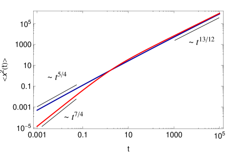
Figure 1: Graphical representation of the second moment (3.3) for $a_{1}=a_{2}=1/2$, $\mu_{1}=13/12$ and $\mu_{2}=5/4$ (blue line), $\mu_{2}=7/4$ (red line). The crossover from power-law behavior with exponent $\mu_{2}$ to power-law behavior with an exponent $\mu_{1}$ is obvious.

Remark 7. We note that for the case $0<\mu_{1}<1$ and $1<\mu_{2}<2$ we are not able to prove the non-negativity of the solution. Thus, whether such diffusion-wave equation for the PDF may exist or not is still an open question.

3.4 Fractional diffusion-wave equation with $N$ fractional exponents

A natural generalization of the previous case is a memory kernel of the form

$$\eta(t)=\sum_{j=1}^{N}\alpha_{j}\frac{t^{1-\mu_{j}}}{\Gamma(2-\mu_{j})},$$ (50)

where $0<\mu_{1}<\mu_{2}<\dots<\mu_{N}<2$. From (50) we find $\hat{\eta}(s)=\sum_{j=1}^{N}\alpha_{j}s^{\mu_{j}-2}$. Thus, from Eq. (2) with kernel (50) and $1<\mu_{j}<2$ we get

$$\sum_{j=1}^{N}\alpha_{j}{{}_{C}}D_{0+}^{\mu_{j}}W(x,t)=\frac{\partial^{2}}{\partial x^{2}}W(x,t),$$ (51)

where ${{}_{C}}D_{0+}^{\mu_{j}}$ is the Caputo fractional derivative (5) of order $1<\mu_{j}<2$. For $0<\lambda<1$, $0<\mu_{j}<1$, $j=1,2,\dots,N$ we get

$$\sum_{j=1}^{N}\alpha_{j}\int_{0}^{t}\frac{(t-t^{\prime})^{1-\mu_{j}}}{\Gamma(2-\mu_{j})}\frac{\partial^{2}}{\partial t^{\prime 2}}W(x,t^{\prime})\,dt^{\prime}=\frac{\partial^{2}}{\partial x^{2}}W(x,t).$$ (52)

The solutions of Eq. (51) with $1<\mu_{1}<\mu_{2}<\dots<\mu_{N}<2$ is non-negative since

$$\hat{\eta}(s)=\sum_{j=1}^{N}\alpha_{j}s^{\mu_{j}-2}$$

is a SF (see property (c) in Section 2.1.2.), that is $\sqrt{\eta(s)}$ a SF too (see property (g) in Section 2.1.4.), which means that $\sqrt{\hat{\eta}(s)}$ is CM. Thus, $s\sqrt{\hat{\eta}(s)}$ is a CBF (see property (h) in Section 2.1.4.), with which we complete the proof of non-negativity of the solution. For the case with $0<\mu_{1}<\mu_{2}<\dots<\mu_{N}<1$ the non-negativity of the solution of Eq. (52) can be shown by using the subordination approach (see Remark 1), that is $s\hat{\eta}(s)=\sum_{j=1}^{N}\alpha_{j}s^{\mu_{j}-1}$ a CM, and $s^{2}\hat{\eta}(s)=\sum_{j=1}^{N}\alpha_{j}s^{\mu_{j}}$ is a BF.

For the MSD we find

$$\left\langle x^{2}(t)\right\rangle=2\,\mathcal{L}^{-1}\left[\frac{s^{-1}}{\sum_{j=1}^{N}\alpha_{j}s^{\mu_{j}}}\right](t)$$

$$=\frac{2}{\alpha_{N}}t^{\mu_{N}}E_{(\mu_{N}-\mu_{1},\dots,\mu_{N}-\mu_{N-1}),\mu_{N}+1}\left(-\frac{\alpha_{1}}{\alpha_{N}}t^{\mu_{N}-\mu_{1}},\dots,-\frac{\alpha_{N-1}}{\alpha_{N}}t^{\mu_{N}-\mu_{N-1}}\right),$$

where $E_{(a_{1},a_{2},\dots,a_{N}),b}(z)$ is the multinomial M-L function [30, 25], defined by

$$E_{\left(a_{1},a_{2},\ldots,a_{N}\right),b}\left(z_{1},z_{2},\ldots,z_{N}\right)=\sum_{j=1}^{\infty}\sum_{k_{1}\geq 0,k_{2}\geq 0,\ldots,k_{N}\geq 0}^{k_{1}+k_{2}+\ldots+k_{N}=j} \left(\begin{array}[]{c}j\\ k_{1}\quad k_{2}\quad\ldots\quad k_{N}\end{array}\right)$$ (57)

$$\times\frac{\prod_{i=1}^{N}\left(z_{i}\right)^{k_{i}}}{\Gamma\left(b+\sum_{i=1}^{N}a_{i}k_{i}\right)},$$

where

$$\left(\begin{array}[]{c}j\\ k_{1}\quad k_{2}\quad...\quad k_{N}\end{array}\right)=\frac{j!}{k_{1}!k_{2}!...k_{N}!}$$

are the so-called multinomial coefficients. For the asymptotic behavior of the second moment we get

$$\langle x^{2}(t)\rangle\simeq\left\{\begin{array}[]{c l}\frac{2}{\alpha_{N}}\frac{t^{\mu_{N}}}{\Gamma(1+\mu_{N})},&t\ll 1\\ \frac{2}{\alpha_{1}}\frac{t^{\mu_{1}}}{\Gamma(1+\mu_{1})},&t\gg 1\end{array}\right.$$ (60)

i.e., decelerating superdiffusion for $1<\mu_{1}<\mu_{2}<\dots<\mu_{N}<2$, and decelerating subdiffusion for $0<\mu_{1}<\mu_{2}<\dots<\mu_{N}<1$. We note that the multinomial M-L function plays an important role in the analysis of the generalized Langevin equation [58] and distributed order diffusion equations [53, 56].

Graphical representation of the second moment in case of three power-law memory kernels ($N=3$) is given in Figure 2. It is seen that the second moment in the short time limit behaves as power-law with exponent $\mu_{3}$, which turns to power-law behavior with an exponent $\mu_{1}$. In the intermediate time the behavior is represented by the multinomial M-L function. By introducing more than two power-law memory kernels it is possible to achieve better fit in the intermediate time domain between short and long time asymptotics.

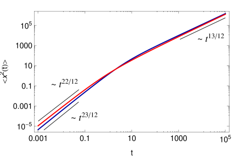
Figure 2: Graphical representation of the second moment (3.4) for $a_{1}=a_{2}=a_{3}=1/3$, $\mu_{1}=13/12$, $\mu_{2}=21/12$, $\mu_{3}=23/12$ (blue line), $\mu_{1}=13/12$, $\mu_{2}=15/12$, $\mu_{3}=22/12$ (red line).

3.5 Uniformly distributed order memory kernel

Next we consider uniformly distributed memory kernel

$$\eta(t)=\int_{1}^{2}\frac{t^{1-\lambda}}{\Gamma(2-\lambda)}\,d\lambda,$$

that corresponds to $p(\lambda)=1$ in Eq. (4). Equation (2) then reads

$$\int_{0}^{t}\int_{1}^{2}\frac{(t-t^{\prime})^{1-\lambda}}{\Gamma(2-\lambda)}\frac{\partial^{2}}{\partial t^{\prime 2}}W(x,t^{\prime})\,d\lambda{d}t^{\prime}=\frac{\partial^{2}}{\partial x^{2}}W(x,t),$$ (61)

i.e.,

$$\int_{1}^{2}{{}_{C}}D_{0+}^{\lambda}W(x,t)\,d\lambda=\frac{\partial^{2}}{\partial x^{2}}W(x,t),$$ (62)

where ${{}_{C}}D_{0+}^{\lambda}$ is the Caputo fractional derivative of the order $1<\lambda<2$.

Let us show the non-negativity of the solution. The function

$$\hat{\eta}(s)=\int_{1}^{2}p(\lambda)s^{\lambda-2}\,d\lambda$$

is a SF since the function $\sum_{j}p_{j}s^{\lambda_{j}-2}$ with $p_{j}\geq 0$ and $1<\lambda_{j}\leq 2$ is a SF (see property (c) in Section 2.1.2.), and a pointwise limit of this linear combination $\eta(s)=\int_{0}^{1}p(\lambda)s^{\lambda-2}\,d\lambda$ is a SF too. Therefore, $\sqrt{\hat{\eta}(s)}$ is a SF as well, since a composition of CBF and SF is a SF (see property (g) in Section 2.1.4.), and thus it is CM. Therefore, $s\sqrt{\hat{\eta}(s)}$ is CBF (if $c(x)$ is a CBF, then $c(x)/x$ is a SF (see property (h) in Section 2.1.4.), which means that the solution of the equation (62) is non-negative.

From the solution in Laplace space,

$$\hat{W}(x,s)=\frac{1}{2s}\left(s\sqrt{\frac{s-1}{s\log{s}}}\right)\exp\left(-s\sqrt{\frac{s-1}{s\log{s}}}|x|\right),$$ (63)

by applying the Tauberian theorem for slowly varying functions  [16] we can obtain the asymptotic behavior of $W(x,t)$ in the short and long time limit. This theorem states that if some function $r(t)$, $t\geq 0$, has the Laplace transform $\hat{r}(s)$ whose asymptotics behaves as

$$\hat{r}(s)\simeq s^{-\rho}L\left(\frac{1}{s}\right),\quad s\rightarrow 0,\quad\rho\geq 0,$$ (64)

then

$$r(t)=\mathcal{L}^{-1}\left[\hat{r}(s)\right]\simeq\frac{1}{\Gamma(\rho)}t^{\rho-1}L(t),\quad t\rightarrow\infty.$$ (65)

Here $L(t)$ is a slowly varying function at infinity, i.e.,

$$\lim_{t\rightarrow\infty}\frac{L(at)}{L(t)}=1,$$

for any $a>0$. The theorem is also valid if $s$ and $t$ are interchanged, that is $s\rightarrow\infty$ and $t\rightarrow 0$ [16]. The value of $\rho$ is equal to $0$ and $1/2$ for short and long time limit respectively. Therefore, from Eq. (63) we find

$$W(x,t)\simeq\left\{\begin{array}[]{c l}\frac{1}{\sqrt{4t^{2}\log{\frac{1}{t}}}}\exp\left(-\frac{|x|}{\sqrt{t^{2}\log{\frac{1}{t}}}}\right),&t\ll 1,\\ \frac{1}{\sqrt{4t\log{t}}}\exp\left(-\frac{|x|}{\sqrt{t\log{t}}}\right),&t\gg 1.\end{array}\right.$$ (68)

The MSD reads

$$\left\langle x^{2}(t)\right\rangle=2\,\mathcal{L}^{-1}\left[\frac{\log{s}}{s^{2}(s-1)}\right](t).$$ (69)

From here, by applying the Tauberian theorem for slowly varying functions, we obtain

$$\langle x^{2}(t)\rangle\simeq\left\{\begin{array}[]{c l}2\,\mathcal{L}^{-1}\left[s^{-3}\log{s}\right](t)\simeq t^{2}\log\frac{1}{t},&t\ll 1,\\ 2\,\mathcal{L}^{-1}\left[s^{-2}\log\frac{1}{s}\right](t)=2\,t\left(-1+\gamma+\log{t}\right)\simeq 2\,t\log{t},&t\gg 1.\end{array}\right.$$ (72)

Therefore, the behavior of the MSD is weakly superballistic at short times and weakly superdiffusive at long times. Interestingly, the MSD (72) for the diffusion–wave equation (62) in comparison to the MSD for the diffusion equation with uniformly distributed order memory kernel [10, 9], has an additional multiplicative term $t$ for both short and long times.

3.6 Truncated power-law memory kernel

Next we present results in case of a truncated power-law memory kernel of the form

$$\eta(t)=e^{-bt}\frac{t^{1-\mu}}{\Gamma(2-\mu)},$$ (74)

where $b>0$, and $1\leq\mu<2$. Its Laplace transform is given by $\hat{\eta}(s)=(s+b)^{\mu-2}$, where we use the shift rule of the Laplace transform

$$\mathcal{L}\left[f(t)e^{-at}\right](s)=\hat{F}(s+a),\quad\mathrm{with}\quad\mathcal{L}\left[f(t)\right](s)=\hat{F}(s).$$ (75)

The solution of the diffusion-wave equation with the truncated memory kernel (74) is non-negative for $1\leq\mu<2$ since $\hat{\eta}(s)=(s+b)^{\mu-2}$ is a SF as a composition of SF ($s^{\mu-2}$, $1\leq\mu<2$) and CBF ($s+b$) (see property (f) in Section 2.1.4.). Therefore $\sqrt{\eta(s)}$ is a SF too, with which we complete the proof.

From the solution in Laplace space we find the exact solution in the following form

$$W(x,t) = \mathcal{L}^{-1}\left[\frac{1}{2s}(s+b)^{\mu/2}\exp\left(-(s+b)^{\mu/2}|x|\right)\right](x,t)$$ (78)

$$= {{}_{RL}}I_{t}^{1}\left(\frac{e^{-bt}}{2|x|t}H_{1,1}^{1,0}\left[\frac{|x|}{t^{\mu/2}}\left|\begin{array}[]{c l}(0,\mu/2)\\ (0,1)\end{array}\right.\right]\right),$$

where we use the relation between the exponential and the Fox $H$-function [39]

$$e^{-z}=H_{0,1}^{1,0}\left[z\left|\begin{array}[]{l}-\\ (0,1)\end{array}\right.\right],$$ (81)

the shift rule (75), and the Laplace transform formula [39]

$$\mathcal{L}^{-1}\left[s^{-\rho}H_{p,q}^{m,n}\left[zs^{\sigma}\left|\begin{array}[]{c l}(a_{p},A_{p})\\ (b_{q},B_{q})\end{array}\right.\right]\right](t)=t^{\rho-1}H_{p+1,q}^{m,n}\left[zt^{-\sigma}\left|\begin{array}[]{c l}(a_{p},A_{p}),(\rho,\sigma)\\ (b_{q},B_{q})\end{array}\right.\right],$$ (86)

where $\sigma>0$, $\Re(s)>0$, $\Re\left(\rho+\sigma\max_{1\leq j\leq n}\left(\frac{1-a_{j}}{A_{j}}\right)\right)>0$, $|\arg(z)|<\pi\theta_{1}/2$, $\theta_{1}>0$, $\theta_{1}=\theta-a$.

From Eq. (13) for the second moment we obtain

$$\left\langle x^{2}(t)\right\rangle=2\,\mathcal{L}^{-1}\left[s^{-3}(s+b)^{2-\mu}\right](t)=2\,{{}_{RL}}I_{t}^{3}\left(e^{-bt}\frac{t^{-3+\mu}}{\Gamma(-2+\mu)}\right),$$ (88)

where

$${{}_{RL}I_{t}^{\alpha}}f(t)=\frac{1}{\Gamma(\alpha)}\int_{0}^{t}(t-t^{\prime})^{\alpha-1}f(t^{\prime})\,dt^{\prime}$$ (89)

is the Riemann-Liouville integral, whose Laplace transform is given by $\mathcal{L}\left[{{}_{RL}I_{t}^{\alpha}}f(t)\right](s)=s^{-\alpha}\mathcal{L}\left[f(t)\right](s)$ [50]. For the asymptotic behavior of the second moment we use the Tauberian theorem [16], which states that if the asymptotic behavior of $r(t)$ for $t\rightarrow\infty$ is given by

$$r(t)\simeq t^{-\alpha},\quad t\rightarrow\infty,$$ (90)

then, the corresponding Laplace pair $\hat{r}(s)=\mathcal{L}[r(t)](s)$ has the following behavior for $s\rightarrow 0$

$$\hat{r}(s)\simeq\Gamma(1-\alpha)s^{\alpha-1},\quad s\rightarrow 0,$$ (91)

and vice-versa, ensuring that $r(t)$ is non-negative and monotone function at infinity [16]. Thus, we find

$$\langle x^{2}(t)\rangle\simeq\left\{\begin{array}[]{c l}2\,\frac{t^{\mu}}{\Gamma(1+\mu)},&t\ll 1,\\ b^{2-\mu}t^{2},&t\gg 1,\end{array}\right.$$ (94)

which means that the process switches from superdiffusive behavior to ballistic motion in the case with $1<\mu<2$, and from normal diffusion to ballistic motion in the case with $\mu=1$. The fact that we encounter accelerating superdiffusion caused by truncation of the power law kernel in the diffusion-wave equation is not surprising. Indeed, it is analogous to the transition from subdiffusion to normal diffusion described by the fractional diffusion equation with truncated power law kernel in the Caputo form [53, 57]. As in diffusion equation the truncation naturally leads to a normal diffusion at long times, in diffusion–wave equation the truncation results in the long–time ballistic behavior.

3.7 Truncated Mittag-Leffler memory kernel

Here we consider tempered M-L memory kernel of form

$$\eta(t)=e^{-bt}t^{\beta-1}E_{\alpha,\beta}^{\delta}\left(-\nu t^{\alpha}\right),$$ (95)

where $\alpha\delta<\beta<1$, and $E_{\alpha,\beta}^{\delta}(z)$ is the three parameter M-L function [51] (for details on three parameter M-L function we refer to [17, 66])

$$E_{\alpha,\beta}^{\delta}(z)=\sum_{k=0}^{\infty}\frac{(\delta)_{k}}{\Gamma(\alpha k+\beta)}\frac{z^{k}}{k!},$$ (96)

$\beta,\delta,z\in\mathrm{C}$, $\Re(\alpha)>0$, and $(\delta)_{k}$ is the Pochhammer symbol $(\delta)_{0}=1$, $(\delta)_{k}=\frac{\Gamma(\delta+k)}{\Gamma(\delta)}$. The asymptotic behavior of the three parameter M-L function for large arguments follows from the formula [17, 56]

$$E_{\alpha,\beta}^{\delta}(-t^{\alpha})=\frac{t^{-\alpha\delta}}{\Gamma(\delta)}\sum_{n=0}^{\infty}\frac{\Gamma(\delta+n)}{\Gamma(\beta-\alpha(\delta+n)}\frac{(-t^{\alpha})^{-n}}{n!},\quad t\gg 1,$$ (97)

for $0<\alpha<2$. The Laplace transform of the memory kernel becomes

$$\hat{\eta}(s)=\frac{(s+b)^{\alpha\delta-\beta}}{\left[(s+b)^{\alpha}+\nu\right]^{\delta}},$$

where we use the Laplace transform formula [51]

$$\mathcal{L}\left[t^{\beta-1}E_{\alpha,\beta}^{\delta}\left(-\lambda t^{\alpha}\right)\right](s)=\frac{s^{\alpha\delta-\beta}}{(s^{\alpha}+\lambda)^{\delta}},\quad|\lambda/s^{\alpha}|<1.$$ (98)

Therefore, the generalized diffusion-wave equation has the form

$$\int_{0}^{t}(t-t^{\prime})^{\beta-1}E_{\alpha,\beta}^{\delta}\left(-\nu[t-t^{\prime}]^{\alpha}\right)\frac{\partial^{2}}{\partial t^{\prime 2}}W(x,t^{\prime})\,dt^{\prime}=\frac{\partial^{2}}{\partial x^{2}}W(x,t).$$ (99)

In order to find the parameters’ constraints, for which the solution of Eq. (99) is non-negative, we notice that $\hat{\eta}(s)$ is a SF (and thus CM) if both functions $(s+b)^{-(\beta-\alpha\delta)}$ and $\left[(s+b)^{\alpha}+\nu\right]^{-\delta}$ are SFs. The first one is a SF if $0<\beta-\alpha\delta<1$ and the second one – if $0<\alpha\delta<1$. Therefore, we use $0<\alpha\delta<\beta<1$.

For the MSD we find

$$\left\langle x^{2}(t)\right\rangle = 2\,\mathcal{L}^{-1}\left[s^{-3}\frac{(s+b)^{-\alpha\delta+\beta}}{\left[(s+b)^{\alpha}+\nu\right]^{-\delta}}\right](t)$$ (100)

$$= 2\,{{}_{RL}}I_{t}^{3}\left(e^{-bt}t^{-\beta-1}E_{\alpha,-\beta}^{-\delta}\left(-\nu t^{\alpha}\right)\right).$$

Again, by using the Tauberian theorem [16], for the short and long time limit we find

$$\langle x^{2}(t)\rangle\simeq\left\{\begin{array}[]{c l}2\,t^{2-\beta}/\Gamma(3-\beta),&t\ll 1,\\ b^{-\alpha\delta+\beta}\left(b^{\alpha}+\nu\right)^{\delta}t^{2},&t\gg 1.\end{array}\right.$$ (103)

Therefore, truncation (tempering) of the M-L kernel causes ballistic motion in the long time limit, which follows the superdiffusive initial behavior. Here we note that tempered M-L memory kernel has been introduced in the analysis of the generalized Langevin equation [29], where the crossover from initial subdiffusion to normal diffusion is observed. The case with no truncation ($b=0$) for the second moment yields $\left\langle x^{2}(t)\right\rangle=2t^{2-\beta}E_{\alpha,3-\beta}^{-\delta}\left(-\nu t^{\alpha}\right)$, which in the long time limit behaves as $\left\langle x^{2}(t)\right\rangle\simeq t^{2+\alpha\delta-\beta}$.

Graphical representation of the second moment (100) is given in Figure 3. The influence of tempering on particle behavior is clearly observed. Comparison with the asymptotic behaviors in the short and long time limit is given in Figure 4.

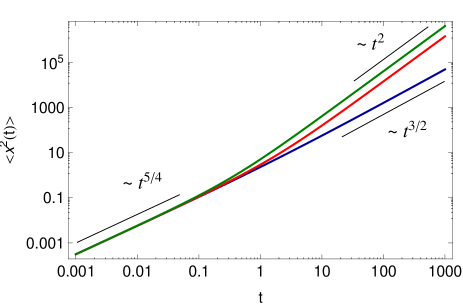
Figure 3: Graphical representation of the second moment (100) for the case of truncated M-L memory kernel for $\alpha=\delta=1/2$, $\beta=3/4$, $\nu=1$ and $b=0$ (blue line), $b=1$ (red line), $b=5$ (green line).

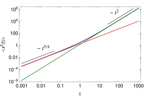
Figure 4: Graphical representation of (100) for $\alpha=\delta=1/2$, $\beta=3/4$, $\nu=1$, $b=1$ (blue line). The short time limit $\left\langle x^{2}(t)\right\rangle\simeq 2\,t^{2-\beta}/\Gamma(3-\beta)$ (red line) and long time limit $\left\langle x^{2}(t)\right\rangle\simeq t^{2}b^{-\alpha\delta+\beta}\left(b^{\alpha}+\nu\right)^{\delta}$ (green line) are in excellent agreement with the exact result.

3.8 Case with regularized Prabhakar derivative

Let us now consider the regularized Prabhakar derivative defined by [18]

$${{}_{C}}\mathcal{D}_{\rho,-\nu,t\,}^{\delta,\mu}f(t)=\left(\mathcal{E}_{\rho,m-\mu,-\nu,t\,}^{-\delta}\frac{d^{m}}{dt^{m}}f\right)(t),$$ (104)

where $\mu,\nu,\delta,\rho\in C$, $\Re(\mu)>0$, $\Re(\rho)>0$, $m=[\mu]+1$, and

$$\left(\mathcal{E}_{\rho,m-\mu,-\nu,t\,}^{-\delta}f\right)(t)=\int_{0}^{t}(t-t^{\prime})^{m-\mu-1}E_{\rho,m-\mu}^{-\delta}\left(-\nu(t-t^{\prime})^{\rho}\right)f(t^{\prime})\,dt^{\prime}$$ (105)

is the Prabhakar integral [51]. Therefore, for $1<\mu<2$ ($m=2$) we have

$${{}_{C}}\mathcal{D}_{\rho,-\nu,t\,}^{\delta,\mu}f(t) = \left(\mathcal{E}_{\rho,2-\mu,-\nu,t\,}^{-\delta}\frac{d^{2}}{dt^{2}}f\right)(t)=\int_{0}^{t}(t-t^{\prime})^{1-\mu}E_{\rho,2-\mu}^{-\delta}\left(-\nu(t-t^{\prime})^{\rho}\right)\frac{d^{2}}{dt^{\prime 2}}f(t^{\prime})\,dt^{\prime}$$ (106)

$$= \int_{0}^{t}\eta(t-t^{\prime})\frac{d^{2}}{dt^{\prime 2}}f(t^{\prime})\,dt^{\prime},$$

where

$$\eta(t)=t^{1-\mu}E_{\rho,2-\mu}^{-\delta}\left(-\nu t^{\rho}\right),\quad 1<\mu<2,$$ (107)

that is the kernel on the left hand side of Eq. (2). This resembles the case considered in subsection III.G, see Eq. (95), if $b=0$, however, in that previous case the MSD asymptotics at long times is determined by $b$, see Eq. (103). This is why the kernel (107) is considered separately. We also use that $0<\rho<1$ and $0<\delta<1$. The generalized diffusion-wave equation then becomes

$${{}_{C}}\mathcal{D}_{\rho,-\nu,t\,}^{\delta,\mu}W(x,t)=\frac{\partial^{2}}{\partial x^{2}}W(x,t).$$ (108)

The Prabhakar derivative has been introduced and applied to fractional Poisson processes in [18], and further used in viscoelastic theory [19, 20, 21], fractional differential filtration dynamics [7], and generalized Langevin equation [52]. Moreover, the fractional diffusion equation with regularized Prabhakar derivative has been recently derived from the continuous time random walk theory [54].

The non-negativity of the solution of Eq. (108) can be proven as follows. The function

$$\hat{\eta}(s)=\left(s^{\frac{\mu-2}{\delta}}+\nu s^{\frac{\mu-2}{\delta}-\rho}\right)^{\delta}$$

is a SF if $s^{(\mu-2)/\delta}$ and $s^{(\mu-2)/\delta-\rho}$ are SFs, and $0<\delta<1$ (composition of a CBF and SF is a SF, see property (g) in Section 2.1.4.). Therefore, we obtain that $0<2-\mu<\delta$ and $2-\delta<\mu-\rho\delta<2$. For these values of parameters $\sqrt{\hat{\eta}(s)}$ is a SF as well, with which we show the non-negativity of the solution.

Thus, for the second moment we obtain

$$\left\langle x^{2}(t)\right\rangle = 2\,\mathcal{L}^{-1}\left[\frac{s^{-3}}{s^{-\rho\delta+\mu-2}(s^{\rho}+\nu)^{\delta}}\right](t)=2\,\mathcal{L}^{-1}\left[\frac{s^{-1+\rho\delta-\mu}}{(s^{\rho}+\nu)^{\delta}}\right](t)$$ (109)

$$= 2\,t^{\mu}E_{\rho,\mu+1}^{\delta}\left(-\nu t^{\rho}\right).$$

From here, by using Eq. (97), we find the asymptotic behavior in the short and long time limit,

$$\langle x^{2}(t)\rangle\simeq\left\{\begin{array}[]{c l}2\,t^{\mu}/\Gamma(1+\mu),&t\ll 1,\\ 2\,t^{\mu-\rho\delta}/\Gamma(1+\mu-\rho\delta),&t\gg 1,\end{array}\right.$$ (112)

which implies that the random motion shows decelerating superdiffusive behavior.

3.9 Distributed order regularized Prabhakar derivative

Further, for the first time in the literature we introduce the distributed order M-L memory kernel of the form

$$\eta(t)=\int_{1}^{2}t^{1-\mu}E_{\rho,2-\mu}^{-\delta}\left(-\nu t^{\rho}\right)\,d\mu,$$ (113)

where $0<\mu,\rho,\delta<1$, $0<2-\mu<\delta$ and $2-\delta<\mu-\rho\delta<2$. The generalized diffusion-wave equation becomes distributed order wave equation with regularized Prabhakar derivative,

$$\int_{1}^{2}{{}_{C}}\mathcal{D}_{\rho,-\nu,t\,}^{\delta,\mu}W(x,t)\,d\mu=\frac{\partial^{2}}{\partial x^{2}}W(x,t).$$ (114)

Note that for $\delta=0$ Eq. (114) is reduced to the uniformly distributed order wave equation (62).

From the memory kernel (113) we find that

$$\hat{\eta}(s)=\frac{s-1}{s\log{s}}\left(1+\frac{\nu}{s^{\rho}}\right)^{\delta}.$$ (115)

In order to check the non-negativity of the solution of Eq. (114), we should analyze the function

$$\hat{\eta}(s)=\int_{1}^{2}\left(s^{\frac{\mu-2}{\delta}}+\nu s^{\frac{\mu-2}{\delta}-\rho}\right)^{\delta}\,d\mu.$$

It is a SF for the same restrictions of parameters as those for the diffusion-wave equation with regularized Prabhakar derivative since a pointwise limit of the linear combinations of SFs,

$$\sum_{j}\left(s^{\frac{\mu_{j}-2}{\delta}}+\nu s^{\frac{\mu_{j}-2}{\delta}-\rho}\right)^{\delta}$$

is also SF.

For the MSD we obtain

$$\left\langle x^{2}(t)\right\rangle=2\,\mathcal{L}^{-1}\left[\frac{\log{s}}{s^{2}(s-1)}\left(1+\frac{\nu}{s^{\rho}}\right)^{-\delta}\right](t).$$ (116)

Therefore, from the Tauberian theorem the asymptotics at short and long times read

$$\langle x^{2}(t)\rangle\simeq\left\{\begin{array}[]{c l}2\,\mathcal{L}^{-1}\left[\frac{\log{s}}{s^{3}}\right](t)\simeq t^{2}\log\frac{1}{t},&t\ll 1,\\ \frac{2}{\nu^{\delta}}\mathcal{L}^{-1}\left[\frac{\log{\frac{1}{s}}}{s^{2-\rho\delta}}\right](t)\simeq\frac{2}{\nu^{\delta}}\frac{t^{1-\rho\delta}}{\Gamma(2-\rho\delta)}\log{t},&t\gg 1,\end{array}\right.$$ (119)

and thus, the random motion is weakly superballistic at short times and weakly subdiffusive at long times since $0<1-\rho\delta<1$.

4 Discussion: The role of the non-zero second initial condition for the generalized diffusion-wave equation (2)

Let us now analyze the solution of the generalized diffusion-wave equation (2), which we denote as $W^{\ast}(x,t)$, with non-zero second initial condition, for example, $\frac{\partial}{\partial t}W^{\ast}(x,0)=\varphi(x)$, and $W^{\ast}(x,0)=\delta(x)$. The solution in the Fourier-Laplace space reads

$$\tilde{\hat{W}}^{\ast}(\kappa,s)=\frac{s\hat{\eta}(s)}{s^{2}\hat{\eta}(s)+\kappa^{2}}+\frac{1}{s}\frac{s\hat{\eta}(s)}{s^{2}\hat{\eta}(s)+\kappa^{2}}\tilde{\varphi}(\kappa)=\hat{W}(\kappa,s)\left[1+s^{-1}\tilde{\varphi}(\kappa)\right],$$

where $\tilde{\varphi}(\kappa)=\mathcal{F}\left[\varphi(x)\right]$. Therefore, by inverse Fourier transformation we find

$$\hat{W}^{\ast}(x,s)=W(x,s)+s^{-1}\int_{-\infty}^{\infty}W(x-\xi,s)\varphi(\xi)\,d\xi,$$ (121)

from which by inverse Laplace transform we find the exact solution

$$W^{\ast}(x,t)=W(x,t)+\int_{0}^{t}\left[\int_{-\infty}^{\infty}W(x-\xi,t)\varphi(\xi)\,d\xi\right]dt^{\prime}.$$ (122)

From Eq. (4) we find that

$$\int_{-\infty}^{\infty}W(x,t)\,dx=1+\tilde{\varphi}(\kappa=0)\,t,$$

therefore, in order for $W(x,t)$ to be normalized to $1$, we need to have $\tilde{\varphi}(\kappa=0)=0$.

Furthermore, for the the second moment we obtain

$$\left\langle x^{2}(t)\right\rangle=2\,\mathcal{L}^{-1}\left[\frac{1}{s^{3}\hat{\eta}(s)}\right](t)-\tilde{\varphi}^{\prime\prime}(\kappa=0)\,t.$$ (123)

By comparison with the MSD given by Eq. (13) we see that the additional term appears which is linear in time. From the previous analysis of the second moment for zero second initial condition, this term is negligible in the long time limit in case of superdiffusion, and in the short time limit in case of subdiffusion, in the corresponding model with zero second initial condition. It also follows from Eq. (80) that there is a restriction such that the obtained second moment from the PDF must be positive. We also note that additional restrictions will appear from the requirement that all even moments must be non-negative $\left\langle x^{2n}(t)\right\rangle\geq 0$. Thus, the case with the non-zero second initial condition looks non-trivial, and it is reasonable to address this issue for each particular physical situation separately.

5 Summary

We study generalized diffusion-wave equation with a general memory kernel, which brings as a particular case the distributed order time fractional diffusion-wave equation considered earlier. We give the general form of the solution and find the conditions under which it is non-negative for various particular model forms of the memory kernel. For these kernels we also calculated the mean squared displacements and show that the models suggested may describe multi-scaling diffusion processes characterized by different time exponents for different time intervals. The results are summarized in Table 1. We thus obtain a flexible tool which can be applied for the description of diverse diffusion phenomena in complex systems, which demonstrate a non-monoscaling behavior, that is transitions between different diffusion regimes. Of course, in each particular application of these models the physical background should be discussed, for example, the existence of a relevant continuous time random walk description, or the particular form of the second initial condition as discussed in Section 4. We note that a very different model based on the Langevin equation with generalized memory kernel has been studied very recently, which also leads to different crossovers between the diffusion regimes [47].

Table 1: Behavior of the MSD in the short and long time limit obtained from the generalized diffusion-wave equation (2), $\int_{0}^{t}\eta(t-t^{\prime})\frac{\partial^{2}}{\partial t^{\prime 2}}W(x,t^{\prime})\,\mathrm{d}t^{\prime}=\frac{\partial^{2}}{\partial x^{2}}W(x,t)$, for different forms of the memory kernel $\eta(t)$.

$\quad\eta(t)\quad$	$\quad\left\langle x^{2}(t)\right\rangle,\quad t\ll 1\quad$	$\quad\left\langle x^{2}(t)\right\rangle,\quad t\gg 1\quad$
$\quad\delta(t)\quad$	$\quad\sim t^{2}$	$\quad\sim t^{2}$
$\quad\frac{t^{1-\mu}}{\Gamma(2-\mu)},\quad 0<\mu<2\quad$	$\quad\sim t^{\mu}$	$\quad\sim t^{\mu}$
$\begin{array}[]{c l}&\alpha_{1}\frac{t^{1-\mu_{1}}}{\Gamma(2-\mu_{1})}+\alpha_{2}\frac{t^{1-\mu_{2}}}{\Gamma(2-\mu_{2})},\\ &1<\mu_{1}<\mu_{2}<2\quad\textrm{or}\quad 0<\mu_{1}<\mu_{2}<1\end{array}$	$\quad\sim t^{\mu_{2}}$	$\quad\sim t^{\mu_{1}}$
$\begin{array}[]{c l}&\sum_{j=1}^{N}\alpha_{j}\frac{t^{1-\mu_{j}}}{\Gamma(2-\mu_{j})},\\ &1<\mu_{1}<\dots<\mu_{N}<2\quad\textrm{or}\\ &0<\mu_{1}<\dots<\mu_{N}<1\end{array}$	$\quad\sim t^{\mu_{N}}$	$\quad\sim t^{\mu_{1}}$
$\quad\int_{1}^{2}\frac{t^{1-\lambda}}{\Gamma(2-\lambda)}\,\mathrm{d}\lambda,\quad 1<\lambda<2\quad$	$\quad\sim t^{2}\log{\frac{1}{t}}$	$\quad\sim t\log{t}$
$\quad e^{-bt}\frac{t^{1-\mu}}{\Gamma(2-\mu)},\quad 1<\mu<2,\quad b>0\quad$	$\quad\sim t^{\mu}$	$\quad\sim t^{2}$
$\begin{array}[]{c l}&e^{-bt}t^{\beta-1}E_{\alpha,\beta}^{\delta}\left(-\nu t^{\alpha}\right),\quad 0<\alpha\delta<\beta<1,\\ &\nu>0,\quad b>0\end{array}$	$\quad\sim t^{2-\beta}$	$\quad\sim t^{2}$
$\begin{array}[]{c l}&t^{1-\mu}E_{\rho,2-\mu}^{-\delta}\left(-\nu t^{\rho}\right),\\ &1<\mu<2,\quad 0<2-\mu<\delta,\\ &2-\delta<\mu-\rho\delta<2\quad 0<\rho,\delta<1\end{array}\quad$	$\quad\sim t^{\mu}$	$\quad\sim t^{\mu-\rho\delta}$
$\begin{array}[]{c l}&\int_{1}^{2}t^{1-\mu}E_{\rho,2-\mu}^{-\delta}\left(-\nu t^{\rho}\right),\\ &1<\mu<2,\quad 0<2-\mu<\delta,\\ &2-\delta<\mu-\rho\delta<2\quad 0<\rho,\delta<1\end{array}$	$\quad\sim t^{2}\log{\frac{1}{t}}$	$\quad\sim t^{1-\rho\delta}\log{t}$

It would be of interest to study the case with distributed order memory kernel of the form $\eta(t)=\int_{0}^{2}p(\lambda){{}_{C}D_{t}^{\lambda}}\,d\lambda$, which is a kind of generalization of the telegrapher’s equation [37, 38, 49]. We also leave for future investigation the corresponding model in the Riemann-Liouville form, which is given by

$$\frac{\partial^{2}}{\partial t^{2}}W(x,t)=\frac{\partial^{2}}{\partial t^{2}}\int_{0}^{t}\zeta(t-t^{\prime})\frac{\partial^{2}}{\partial x^{2}}W(x,t^{\prime})\,dt^{\prime}.$$ (124)

References

References

- [1] Ariel G, Rabani A, Benisty S, Partridge J D, Harshey R M and Be’er A 2015 Nature Comm. 6 8396
- [2] Barkai E, Garini Y and Metzler R 2012 Phys. Today 65 29
- [3] Bazhlekova E 2015 Mathematics 2 412
- [4] Bazhlekova E and Bazhlekov I 2018 J. Comput. Appl. Math. 339 179
- [5] Berkowitz B, Cortis A, Dentz M and Scher H 2006 Rev. Geophys. 44 RG2003
- [6] Brockmann D, Hufnagel L and Geisel T 2006 Nature 439 462
- [7] Bulavatsky V M 2017 Cybern. Syst. Anal. 53 204
- [8] Caspi A, Granek R and Elbaum M 2000 Phys. Rev. Lett 85 5655
- [9] Chechkin A V, Gorenflo R and Sokolov I M 2002 Phys. Rev. E 66 046129
- [10] Chechkin A V, Klafter J and Sokolov I M 2003 Europhys. Lett. 63 326
- [11] Chechkin A V, Gonchar V, Gorenflo R, Korabel N and Sokolov I M 2008 Phys Rev E 78 021111
- [12] Chechkin A V, Gorenflo R, Sokolov I M and Gonchar V 2003 Fract. Calc. Appl. Anal. 6 259
- [13] Chechkin A, Sokolov I M and Klafter J 2011 in Fractional dynamics: recent advances ed J Klafter, S Lim, R Metzler (Singapore: World Scientific Publishing Company) p 107
- [14] del-Castillo-Negrete D, Carreras B A and Lynch V E 2005 Phys. Rev. Lett. 94 065003
- [15] Compte A and Metzler R 1997 J. Phys. A: Math. Gen. 30 7277
- [16] Feller W 1968 An Introduction to Probability Theory and Its Applications vol II (New York: Wiley)
- [17] Garra R and Garrappa R 2018 Commun. Nonlinear Sci. Numer. Simul. 56 314
- [18] Garra R, Gorenflo R, Polito F and Tomovski Z 2014 Appl. Math. Comput. 242 576
- [19] Garrappa R 2016 Commun. Nonlinear Sci. Numer. Simul. 38 178
- [20] Garrappa R, Mainardi F and Maione G 2016 Fract. Calc. Appl. Anal. 19 1105
- [21] Giusti A and Colombaro I 2018 Commun. Nonlinear Sci. Numer. Simul. 56 138
- [22] Gorenflo R 2015 Commun. Appl. Industr. Math. 6 e-531
- [23] Gorenflo R, Luchko Y and Stojanovic M 2013 Fract. Calc. Appl. Anal. 16 297
- [24] Gorenflo R and Mainardi F 2005 J. Phys.: Conf. Ser. 7 1
- [25] Hilfer R, Luchko Y and Tomovski Z 2009 Fract. Calc. Appl. Anal. 12 299
- [26] Höfling F and Franosch T 2013 Rep. Prog. Phys. 76 046602
- [27] Kochubei A N 2009 J. Phys. A: Math. Theor. 42 315203
- [28] Latora V, Rapisarda A and Ruffo S 1999 Phys. Rev. Lett. 83 2104; Latora V, Rapisarda A and Tsallis C 2001 Phys. Rev. E 64, 056134
- [29] Liemert A, Sandev T and Kantz H 2017 Physica A 466 356
- [30] Luchko Y and Gorenflo R 1999 Acta Math. Vietnamica 24 207
- [31] Luchko Y, Mainardi F and Povstenko Y 2013 Comput. Math. Appl. 66 774
- [32] Mainardi F 1996 Appl. Math. Lett. 9 23
- [33] Mainardi F 2010 Fractional Calculus and Waves in Linear Viscoelesticity: An introduction to Mathematical Models (London: Imperial College Press)
- [34] Mainardi F and Pagnini G 2007 J. Comput. Appl. Math. 207 245
- [35] Mainardi F, Pagnini G and Gorenflo R 2007 Appl. Math. Comput. 187 295
- [36] Masoliver J and Weiss G H 1996 Eur. J. Phys. 17 190
- [37] Masoliver J 2016 Phys. Rev. E 93 052107
- [38] Masoliver J and Lindenberg K 2017 Eur. Phys. J. B 90 107
- [39] Mathai A M, Saxena R K and Haubold H J 2010 The -function: Theory and Applications (New York, Dordrecht, Heidelberg, London: Springer)
- [40] Meerschaert M M, Schilling R L and Sikorskii A 2015 Nonlin. Dyn. 80 1685
- [41] Meerschaert M M, Straka P, Zhou Y and McGough R J 2012 Nonlin. Dyn. 70 1273
- [42] Meroz Y and Sokolov I M 2015 Phys. Rep. 573 1
- [43] Metzler R and Compte A 1999 Physica A 268 454
-
[44]
Metzler R and Klafter J 2000 Phys. Rep. 339 1
Metzler R and Klafter J 2004 J. Phys. A: Math. Gen. 37 R161 - [45] Metzler R, Jeon J -H, Cherstvy A G and Barkai E 2014 Phys. Chem. Chem. Phys. 16 24128
- [46] Metzler R and Nonnemacher T F 1998 Phys. Rev. E 57 6409
- [47] Molina-Garcia D, Sandev T, Safdari H, Pagnini G, Chechkin A and Metzler R 2018 New J. Phys. 20 103027
- [48] Norregaard K, Metzler R, Ritter C M, Berg-Sorensen K and Oddershede L B 2017 Chem. Rev. 117 4342
- [49] Orsingher E and Beghin L 2004 Prob. Theory Rel. Fields 128 141
- [50] Podlubny I 1999 Fractional Differential Equations (San Diego: Academic Press)
- [51] Prabhakar T R 1971 Yokohama Math. J. 19 7
- [52] Sandev T 2017 Mathematics 5 66
- [53] Sandev T, Chechkin A, Kantz H and Metzler R 2015 Fract. Calc. Appl. Anal. 18 1006
- [54] Sandev T, Deng W and Xu P 2018 J. Phys. A: Math. Theor. 51 405002
- [55] Sandev T, Metzler R and Chechkin A 2018 Fract. Calc. Appl. Anal. 21 10
- [56] Sandev T, Chechkin A, Korabel N, Kantz H, Sokolov I M and Metzler R 2015 Phys. Rev. E 92 042117
- [57] Sandev T, Sokolov I M, Metzler R and Chechkin A 2017 Chaos Solitons & Fractals 102 210
- [58] Sandev T and Tomovski Z 2014 Phys. Lett. A 378 1
- [59] Saxton M J and Jacobsen K 1997 Ann. Rev. Biophys. Biomol. Struct. 26 373
- [60] Scher H and Montroll E W 1975 Phys. Rev. B 12 2455
- [61] Schilling R, Song R and Vondracek Z 2010 Bernstein Functions (Berlin: De Gruyter)
- [62] Schneider W R and Wyss W 1989 J. Math. Phys. 30 134
- [63] Sokolov I M, Chechkin A V and Klafter J 2004 Acta Physica Polonica B 35 1323
- [64] Solomon T H, Weeks E R and Swinney H L 1993 Phys. Rev. Lett. 71 3975
- [65] Stanislavsky A, Weron K and Weron A 2008 Phys. Rev. E 78 051106
- [66] Tomovski Z, Pogány T K and Srivastava H M 2014 J. Franklin Inst. 351 5437
- [67] Young W, Pumir A and Pomeau Y 1989 Phys. Fluids A1 462
- [68] Viswanathan G E, da Luz M G E, Raposo E P and Stanley H E 2011 The Physics of Foraging. An Introduction to Random Searches and Biological Encounters (Cambridge: Cambridge University Press)
- [69] Weiss G H 2002 Physica A 311 381
- [70] Wu X -L and Libchaber A 2000 Phys. Rev. Lett. 84 3017
- [71] Zhokh A, Trypolskyi A and Strizhak P 2018 Chem. Phys. 503 71