Ensemble Distribution Distillation

Abstract

Ensembles of models often yield improvements in system performance. These ensemble approaches have also been empirically shown to yield robust measures of uncertainty, and are capable of distinguishing between different forms of uncertainty. However, ensembles come at a computational and memory cost which may be prohibitive for many applications. There has been significant work done on the distillation of an ensemble into a single model. Such approaches decrease computational cost and allow a single model to achieve an accuracy comparable to that of an ensemble. However, information about the diversity of the ensemble, which can yield estimates of different forms of uncertainty, is lost. This work considers the novel task of Ensemble Distribution Distillation (EnD²) — distilling the distribution of the predictions from an ensemble, rather than just the average prediction, into a single model. EnD² enables a single model to retain both the improved classification performance of ensemble distillation as well as information about the diversity of the ensemble, which is useful for uncertainty estimation. A solution for EnD² based on Prior Networks, a class of models which allow a single neural network to explicitly model a distribution over output distributions, is proposed in this work. The properties of EnD² are investigated on both an artificial dataset, and on the CIFAR-10, CIFAR-100 and TinyImageNet datasets, where it is shown that EnD² can approach the classification performance of an ensemble, and outperforms both standard DNNs and Ensemble Distillation on the tasks of misclassification and out-of-distribution input detection.

1 Introduction

Neural Networks (NNs) have emerged as the state-of-the-art approach to a variety of machine learning tasks (LeCun et al., 2015) in domains such as computer vision (Girshick, 2015; Simonyan & Zisserman, 2015; Villegas et al., 2017), natural language processing (Mikolov et al., 2013b; a; 2010), speech recognition (Hinton et al., 2012; Hannun et al., 2014) and bio-informatics (Caruana et al., 2015; Alipanahi et al., 2015). Despite impressive supervised learning performance, NNs tend to make over-confident predictions (Lakshminarayanan et al., 2017) and, until recently, have been unable to provide measures of uncertainty in their predictions. As NNs are increasingly being applied to safety-critical tasks such as medical diagnosis (De Fauw et al., 2018), biometric identification (Schroff et al., 2015) and self driving cars, estimating uncertainty in model’s predictions is crucial, as it enables the safety of an AI system (Amodei et al., 2016) to be improved by acting on the predictions in an informed manner.

Ensembles of NNs are known to yield increased accuracy over a single model (Murphy, 2012), allow useful measures of uncertainty to be derived (Lakshminarayanan et al., 2017), and also provide defense against adversarial attacks (Smith & Gal, 2018). There is both a range of Bayesian Monte-Carlo approaches (Gal & Ghahramani, 2016; Welling & Teh, 2011; Garipov et al., 2018; Maddox et al., 2019), as well as non-Bayesian approaches, such as random-initialization (Lakshminarayanan et al., 2017) and bagging (Murphy, 2012; Osband et al., 2016), to generating ensembles. Crucially, ensemble approaches allow total uncertainty in predictions to be decomposed into knowledge uncertainty and data uncertainty. Data uncertainty is the irreducible uncertainty in predictions which arises due to the complexity, multi-modality and noise in the data. Knowledge uncertainty, also known as epistemic uncertainty (Gal, 2016) or distributional uncertainty (Malinin & Gales, 2018), is uncertainty due to a lack of understanding or knowledge on the part of the model regarding the current input for which the model is making a prediction. This form of uncertainty arises when the test input $\bm{x}^{*}$ comes either from a different distribution than the one that generated the training data or from an in-domain region which is sparsely covered by the training data. Mismatch between the test and training distributions is also known as a dataset shift (Quiñonero-Candela, 2009), and is a situation which often arises for real world problems. Distinguishing between sources of uncertainty is important, as in certain machine learning applications it may be necessary to know not only whether the model is uncertain, but also why. For instance, in active learning, additional training data should be collected from regions with high knowledge uncertainty, but not data uncertainty.

A fundamental limitation of ensembles is that the computational cost of training and, more importantly, inference can be many times greater than that of a single model. One solution to speed up inference is to distill an ensemble of models into a single network to yield the mean predictions of the ensemble (Hinton et al., 2015; Korattikara Balan et al., 2015). However, this collapses an ensemble of conditional distributions over classes into a single point-estimate conditional distribution over classes. As a result, information about the diversity of the ensemble is lost. This prevents measures of knowledge uncertainty, such as mutual information (Malinin & Gales, 2018; Depeweg et al., 2017a), from being estimated.

In this work, we investigate the explicit modelling of the distribution over the ensemble predictions, rather than just the mean, with a single model. This problem — referred to as Ensemble Distribution Distillation (EnD²) — yields a method that preserves both the distributional information and improved classification performance of an ensemble within a single neural network model. It is important to highlight that Ensemble Distribution Distillation is a novel task which, to our knowledge, has not been previously investigated. Here, the goal is to extract as much information as possible from an ensemble of models and retain it within a single, possibly simpler, model. As an initial solution to this problem, this paper makes use of a recently introduced class of models, known as Prior Networks (Malinin & Gales, 2018; 2019), which explicitly model a conditional distribution over categorical distributions by parameterizing a Dirichlet distribution. Within the context of EnD² this effectively allows a single model to emulate the complete ensemble.

The contributions of this work are as follows. Firstly, we define the task of Ensemble Distribution Distillation (EnD²) as a new challenge for machine learning research. Secondly, we propose and evaluate a solution to this problem using Prior Networks. EnD² is initially investigated on artificial data, which allows the behaviour of the models to be visualized. It is shown that distribution-distilled models are able to distinguish between data uncertainty and knowledge uncertainty. Finally, EnD² is evaluated on CIFAR-10, CIFAR-100 and TinyImageNet datasets, where it is shown that EnD² yields models which approach the classification performance of the original ensemble and outperform standard DNNs and regular Ensemble Distillation (EnD) models on the tasks of identifying misclassifications and out-of-distribution (OOD) samples.

2 Ensembles

In this work, a Bayesian viewpoint on ensembles is adopted, as it provides a particularly elegant probabilistic framework, which allows knowledge uncertainty to be linked to Bayesian model uncertainty. However, it is also possible to construct ensembles using a range of non-Bayesian approaches. For example, it is possible to explicitly construct an ensemble of $M$ models by training on the same data with different random seeds (Lakshminarayanan et al., 2017) and/or different model architectures. Alternatively, it is possible to generate ensembles via Bootstrap methods (Murphy, 2012; Osband et al., 2016) in which each model is trained on a re-sampled version of the training data.

The essence of Bayesian methods is to treat the model parameters $\bm{\theta}$ as random variables and place a prior distribution ${\tt p}(\bm{\theta})$ over them to compute a posterior distribution ${\tt p}(\bm{\theta}|\mathcal{D})$ via Bayes’ rule:

$$\begin{split}{\tt p}(\bm{\theta}|\mathcal{D})&=\frac{{\tt p}(\mathcal{D}|\bm{\theta}){\tt p}(\bm{\theta})}{{\tt p}(\mathcal{D})}\propto{\tt p}(\mathcal{D}|\bm{\theta}){\tt p}(\bm{\theta})\end{split}$$ (1)

Here, model uncertainty is captured in the posterior distribution ${\tt p}(\bm{\theta}|\mathcal{D})$. Consider an ensemble of models $\{{\tt P}(y|\bm{x}^{*},\bm{\theta}^{(m)})\}_{m=1}^{M}$ sampled from the posterior:

$$\begin{split}\big{\{}{\tt P}(y|\bm{x}^{*},\bm{\theta}^{(m)})\big{\}}_{m=1}^{M}\rightarrow&\big{\{}{\tt P}(y|\bm{\pi}^{(m)})\big{\}}_{m=1}^{M},\quad\bm{\pi}^{(m)}=\ \bm{f}(\bm{x}^{*};\bm{\theta}^{(m)}),\ \bm{\theta}^{(m)}\sim{\tt p}(\bm{\theta}|\mathcal{D})\end{split}$$ (2)

where $\bm{\pi}$ are the parameters of a categorical distribution $[{\tt P}(y=\omega_{1}),\cdots,{\tt P}(y=\omega_{K})]^{\tt T}$ and $\bm{x}^{*}$ is a test input. The expected predictive distribution, or predictive posterior, for a test input $\bm{x}^{*}$ is obtained by taking the expectation with respect to the model posterior:

$$\begin{split}{\tt P}(y|\bm{x}^{*},\mathcal{D})=&\ \mathbb{E}_{{\tt p}(\bm{\theta}|\mathcal{D})}\big{[}{\tt P}(y|\bm{x}^{*},\bm{\theta})\big{]}\end{split}$$ (3)

Each of the models ${\tt P}(y|\bm{x}^{*},\bm{\theta}^{(m)})$ yields a different estimate of data uncertainty. Uncertainty in predictions due to model uncertainty is expressed as the level of spread, or ‘disagreement’, of an ensemble sampled from the posterior. The aim is to craft a posterior ${\tt p}(\bm{\theta}|\mathcal{D})$, via an appropriate choice of prior ${\tt p}(\bm{\theta})$, which yields an ensemble that exhibits the set of behaviours described in figure 1.

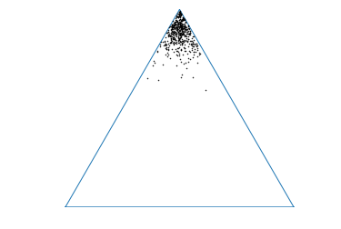
(a) Confident Prediction

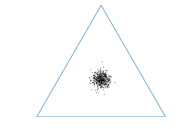
(b) Data Uncertainty

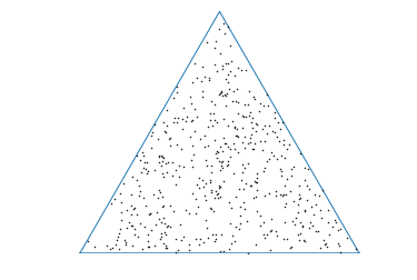
(c) Knowledge Uncertainty

Figure 1: Desired behaviors of a ensemble on a simplex of categorical probabilities.

Specifically, for an in-domain test input $\bm{x}^{*}$, the ensemble should produce a consistent set of predictions with little spread, as described in figure 1(a) and figure 1(b). In other words, the models should agree in their estimates of data uncertainty. On the other hand, for inputs which are different from the training data, the models in the ensemble should ‘disagree’ and produce a diverse set of predictions, as shown in figure 1(c). Ideally, the models should yield increasingly diverse predictions as input $\bm{x}^{*}$ moves further away from the training data. If an input is completely unlike the training data, then the level of disagreement should be significant. Hence, the measures of model uncertainty will capture knowledge uncertainty given an appropriate choice of prior.

Given an ensemble $\big{\{}{\tt P}(y|\bm{x}^{*},\bm{\theta}^{(m)})\big{\}}_{m=1}^{M}$ which exhibits the desired set of behaviours, the entropy of the expected distribution ${\tt P}(y|\bm{x}^{*},\mathcal{D})$ can be used as a measure of total uncertainty in the prediction. Uncertainty in predictions due to knowledge uncertainty can be assessed via measures of the spread, or ‘disagreement’, of the ensemble such as Mutual Information:

$$\begin{split}\underbrace{\mathcal{MI}[y,\bm{\theta}|\bm{x}^{*},\mathcal{D}]}_{Knowledge\ Uncertainty}=&\ \underbrace{\mathcal{H}\big{[}\mathbb{E}_{{\tt p}(\bm{\theta}|\mathcal{D})}[{\tt P}(y|\bm{x}^{*},\bm{\theta})]\big{]}}_{Total\ Uncertainty}-\underbrace{\mathbb{E}_{{\tt p}(\bm{\theta}|\mathcal{D})}\big{[}\mathcal{H}[{\tt P}(y|\bm{x}^{*},\bm{\theta})]\big{]}}_{Expected\ Data\ Uncertainty}\end{split}$$ (4)

This formulation of mutual information allows the total uncertainty to be decomposed into knowledge uncertainty and expected data uncertainty (Depeweg et al., 2017a; b). The entropy of the predictive posterior, or total uncertainty, will be high whenever the model is uncertain - both in regions of severe class overlap and out-of-domain. However, the difference of the entropy of the predictive posterior and the expected entropy of the individual models will be non-zero only if the models disagree. For example, in regions of class overlap, each member of the ensemble will yield a high entropy distribution (figure 1b) - the entropy of the predictive posterior and the expected entropy will be similar and mutual information will be low. In this situation total uncertainty is dominated by data uncertainty. On the other hand, for out-of-domain inputs the ensemble yields diverse distributions over classes such that the predictive posterior is near uniform (figure 1(c)), while the expected entropy of each model may be much lower. In this region of input space the models’ understanding of data is low and, therefore, knowledge uncertainty is high.

3 Ensemble Distribution Distillation

Previous work (Hinton et al., 2015; Korattikara Balan et al., 2015; Wong & Gales, 2017; Wang et al., 2018; Papamakarios, 2015; Buciluǎ et al., 2006) has investigated distilling a single large network into a smaller one and an ensemble of networks into a single neural network. In general, distillation is done by minimizing the KL-divergence between the model and the expected predictive distribution of an ensemble:

$$\begin{split}\mathcal{L}(\bm{\phi},\mathcal{D}_{\tt ens})=&\ \mathbb{E}_{{\tt\hat{p}}(\bm{x})}\Big{[}{\tt KL}\big{[}\mathbb{E}_{{\tt\hat{p}}(\bm{\theta}|\mathcal{D})}[{\tt P}(y|\bm{x};\bm{\theta})]\ ||\ {\tt P}(y|\bm{x};\bm{\phi})]\big{]}\Big{]}\end{split}$$ (5)

This approach essentially aims to train a single model that captures the mean of an ensemble, allowing the model to achieve a higher classification performance at a far lower computational cost. The use of such models for uncertainty estimation was investigated in (Li & Hoiem, 2019; Englesson & Azizpour, 2019). However, the limitation of this approach with regards to uncertainty estimation is that the information about the diversity of the ensemble is lost. As a result, it is no longer possible to decompose total uncertainty into knowledge uncertainty and data uncertainty via mutual information as in equation 4. In this work we propose the task of Ensemble Distribution Distillation, where the goal is to capture not only the mean of the ensemble, but also its diversity. In this section, we outline an initial solution to this task.

An ensemble can be viewed as a set of samples from an implicit distribution of output distributions:

$$\begin{split}\big{\{}{\tt P}(y|\bm{x}^{*},\bm{\theta}^{(m)})\big{\}}_{m=1}^{M}\rightarrow&\big{\{}{\tt P}(y|\bm{\pi}^{(m)})\big{\}}_{m=1}^{M},\quad\bm{\pi}^{(m)}\sim\ {\tt p}(\bm{\pi}|\bm{x}^{*},\mathcal{D})\end{split}$$ (6)

Recently, a new class of models was proposed, called Prior Networks (Malinin & Gales, 2018; 2019), which explicitly parameterize a conditional distribution over output distributions ${\tt p}(\bm{\pi}|\bm{x}^{*};\bm{\hat{\phi}})$ using a single neural network parameterized by a point estimate of the model parameters $\bm{\hat{\phi}}$. Thus, a Prior Network is able to effectively emulate an ensemble, and therefore yield the same measures of uncertainty. A Prior Network ${\tt p}(\bm{\pi}|\bm{x}^{*};\bm{\hat{\phi}})$ models a distribution over categorical output distributions by parameterizing the Dirichlet distribution.

$$\begin{split}{\tt p}(\bm{\pi}|\bm{x};\bm{\hat{\phi}})=&\ {\tt Dir}(\bm{\pi}|\bm{\hat{\alpha}}),\quad\bm{\hat{\alpha}}=\ \bm{f}(\bm{x};\bm{\hat{\phi}}),\quad\hat{\alpha}_{c}>0,\ \hat{\alpha}_{0}=\sum_{c=1}^{K}\hat{\alpha}_{c}\end{split}$$ (7)

The distribution is parameterized by its concentration parameters $\bm{\alpha}$, which can be obtained by placing an exponential function at the output of a Prior Network: $\hat{\alpha}_{c}=e^{\hat{z}_{c}}$, where $\bm{\hat{z}}$ are the logits predicted by the model. While a Prior Network could, in general, parameterize arbitrary distributions over categorical distributions, the Dirichlet is chosen due to its tractable analytic properties, which allow closed form expressions for all measures of uncertainty to be obtained. However, it is important to note that the Dirichlet distribution may be too limited to fully capture the behaviour of an ensemble and other distributions may need to be considered.

In this work we consider how an ensemble, which is a set of samples from an implicit distribution over distributions, can be distribution distilled into an explicit distribution over distributions modelled using a single Prior Network model, ie: $\big{\{}{\tt P}(y|\bm{x};\bm{\theta}^{(m)})\big{\}}_{m=1}^{M}\rightarrow{\tt p}(\bm{\pi}|\bm{x};\bm{\hat{\phi}})$.

This is accomplished in several steps. Firstly, a transfer dataset $\mathcal{D}_{\tt ens}=\{\bm{x}^{(i)},\bm{\pi}^{(i,1:M)}\}_{i=1}^{N}\sim{\tt\hat{p}}(\bm{x},\bm{\pi})$ is composed of the inputs $\bm{x}_{i}$ from the original training set $\mathcal{D}=\{\bm{x}^{(i)},y^{(i)}\}_{i=1}^{N}$ and the categorical distributions $\{\bm{\pi}^{(i,1:M)}\}_{i=1}^{N}$ derived from the ensemble for each input. Secondly, given this transfer set, the model ${\tt p}(\bm{\pi}|\bm{x};\bm{\phi})$ is trained by minimizing the negative log-likelihood of each categorical distribution $\bm{\pi}^{(im)}$:

$$\begin{split}\mathcal{L}(\bm{\phi},\mathcal{D}_{\tt ens})=&\ -\mathbb{E}_{{\tt\hat{p}}(\bm{x})}\big{[}\mathbb{E}_{{\tt\hat{p}}(\bm{\pi}|\bm{x})}[\ln{\tt p}(\bm{\pi}|\bm{x};\bm{\phi})]\big{]}\\ =&\ -\frac{1}{N}\sum_{i=1}^{N}\Big{[}\ln\Gamma(\hat{\alpha}_{0}^{(i)})-\sum_{c=1}^{K}\ln\Gamma(\hat{\alpha}_{c}^{(i)})+\frac{1}{M}\sum_{m=1}^{M}\sum_{c=1}^{K}(\hat{\alpha}_{c}^{(i)}-1)\ln\pi_{c}^{(im)}\Big{]}\end{split}$$ (8)

Thus, Ensemble Distribution Distillation with Prior Networks is a straightforward application of maximum-likelihood estimation. Given a distribution-distilled Prior Network, the predictive distribution is given by the expected categorical distribution $\bm{\hat{\pi}}$ under the Dirichlet prior:

$$\begin{split}{\tt P}(y=\omega_{c}|\bm{x}^{*};\bm{\hat{\phi}})=&\ \mathbb{E}_{{\tt p}(\bm{\pi}|\bm{x}^{*};\bm{\hat{\phi}})}[{\tt P}(y=\omega_{c}|\bm{\pi})]=\ \hat{\pi}_{c}=\ \frac{\hat{\alpha}_{c}}{\sum_{k=1}^{K}\hat{\alpha}_{k}}=\ \frac{e^{\hat{z}_{c}}}{\sum_{k=1}^{K}e^{\hat{z}_{k}}}\end{split}$$ (9)

Separable measures of uncertainty can be obtained by considering the mutual information between the prediction $y$ and the parameters of $\bm{\pi}$ of the categorical:

$$\underbrace{\mathcal{MI}[y,{\tt\bm{\pi}}|\bm{x}^{*};\bm{\hat{\phi}}]}_{Knowledge\ Uncertainty}= \ \underbrace{\mathcal{H}\big{[}\mathbb{E}_{{\tt p}({\tt\bm{\pi}}|\bm{x}^{*};\bm{\hat{\phi}})}[{\tt P}(y|{\tt\bm{\pi}})]\big{]}}_{Total\ Uncertainty}-\underbrace{\mathbb{E}_{{\tt p}({\tt\bm{\pi}}|\bm{x}^{*};\bm{\hat{\phi}})}\big{[}\mathcal{H}[{\tt P}(y|{\tt\bm{\pi}})]\big{]}}_{Expected\ Data\ Uncertainty}$$ (10)

Similar to equation 4, this expression allows total uncertainty, given by the entropy of the expected distribution, to be decomposed into data uncertainty and knowledge uncertainty (Malinin & Gales, 2018). If Ensemble Distribution Distillation is successful, then the measures of uncertainty derivable from a distribution-distilled model should be identical to those derived from the original ensemble.

3.1 Temperature Annealing

Minimization of the negative log-likelihood of the model on the transfer dataset $\mathcal{D}_{\tt ens}=\{\bm{x}^{(i)},\bm{\pi}^{(i,1:M)}\}_{i=1}^{N}$ is equivalent to minimization of the KL-divergence between the model and the empirical distribution ${\tt\hat{p}}(\bm{x},\bm{\pi})$. On training data, this distribution is often ‘sharp’ at one of the corners of the simplex. At the same time, the Dirichlet distribution predicted by the model has its mode near the center of the simplex with little support at the corners at initialization. Thus, the common support between the model and the target empirical distribution is limited. Optimization of the KL-divergence between distributions with limited non-zero common support is particularly difficult. To alleviate this issue, and improve convergence, the proposed solution is to use temperature to ‘heat up’ both distributions and increase common support by moving the modes of both distributions closer together. The empirical distribution is ‘heated up’ by raising the temperature $T$ of the softmax of each model in the ensemble in the same way as in (Hinton et al., 2015). This moves the predictions of the ensemble closer to the center of the simplex and decreases their diversity, making it better modelled by a sharp Dirichlet distribution. The output distribution of the EnD² model ${\tt p}(\bm{\pi}|\bm{x};\bm{\phi})$ is heated up by raising the temperature of the concentration parameters: $\hat{\alpha}_{c}=e^{\hat{z}_{c}/T}$, making support more uniform across the simplex. An annealing schedule is used to re-emphasize the diversity of the empirical distribution and return it to its ‘natural’ state by lowering the temperature down to $1$ as training progresses.

4 Experiments on Artificial Data

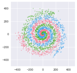
(a) Spiral Dataset

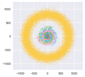
(b) Spiral Dataset with AUX data ( )

Figure 2: 3-spiral dataset with 1000 examples per class

The current section investigates Ensemble Distribution Distillation (EnD²) on an artificial dataset shown in figure 2a. This dataset consists of three spiral arms extending from the center with both increasing noise and distance between the arms. Each arm corresponds to a single class. This dataset is chosen such that it is not linearly separable and requires a powerful model to correctly model the decision boundaries, and also such that there are definite regions of class overlap.

In the following set of experiments, an ensemble of 100 neural networks is constructed by training neural networks from 100 different random initializations. A smaller (sub) ensemble of only 10 neural networks is also considered. The models are trained on 3000 data-points sampled from the spiral dataset, with 1000 examples per class. The classification performance of EnD² is compared to the performance of individual neural networks, the overall ensemble and regular Ensemble Distillation (EnD). The results are presented in table 1.

Table 1: Classification Performance (% Error) on $\mathcal{D}_{test}$ of size 1000, trained on $\mathcal{D}_{trn}$ of size 1000 with 3 spiral classes. Dataset sizes given as number of examples per class.

Num. models	Individual	Ensemble	EnD	EnD2
10	13.21	12.63	12.57	12.52
100		12.37	12.39	12.47

The results show that an ensemble of 10 models has a clear performance gain compared to the mean performance of the individual models. An ensemble of 100 models has a smaller performance gain over an ensemble of only 10 models. Ensemble Distillation (EnD) is able to recover the classification performance of both an ensemble of 10 and 100 models with only very minor degradation in performance. Finally, Ensemble Distribution Distillation is also able to recover most of the performance gain of an ensemble, but with a slightly larger degradation. This is likely due to forcing a single model to learn not only the mean, but also the distribution around it, which likely requires more capacity from the network.

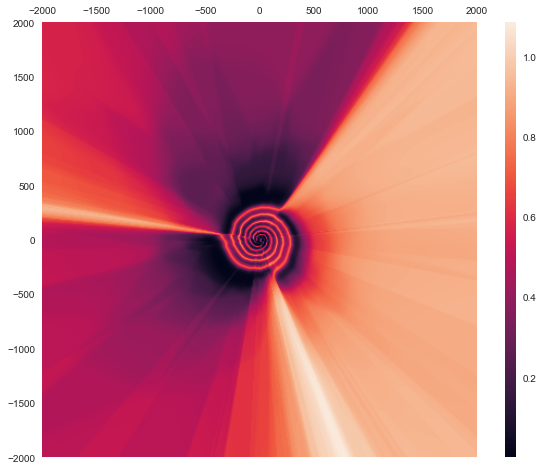
(a) Ensm. Total Uncertainty

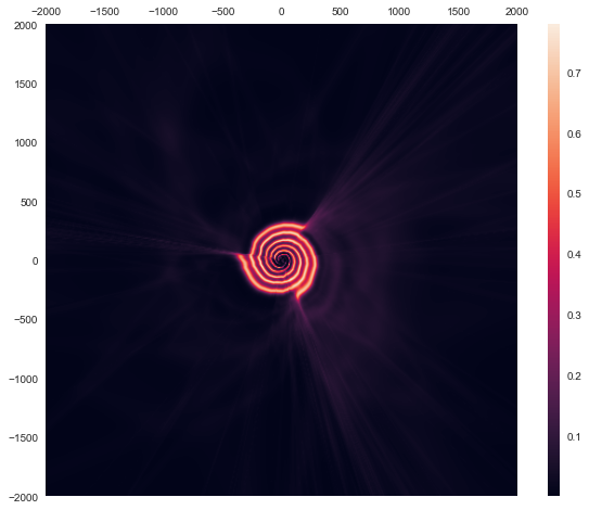
(b) Ensm. Data Uncertainty

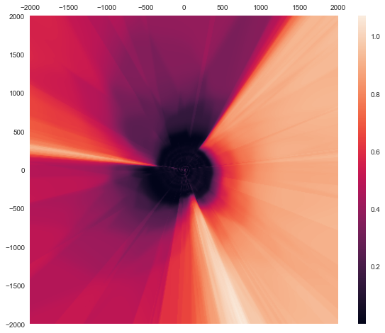
(c) Ensm. Knowledge Uncertainty

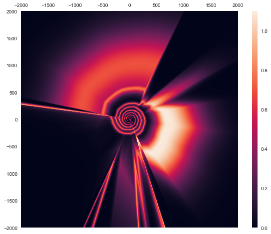
(d) EnD² Total Uncertainty

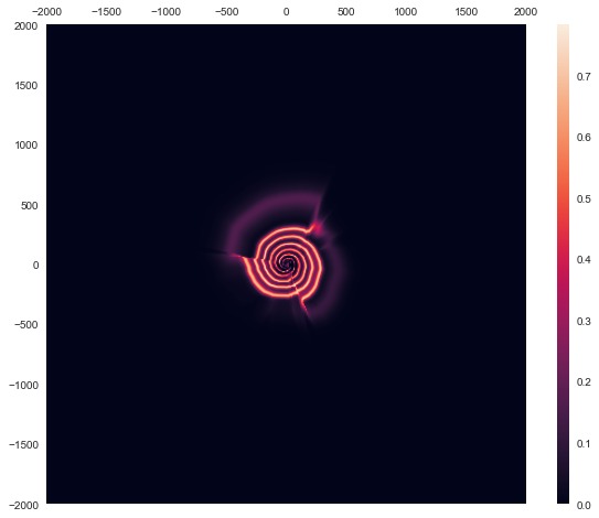
(e) EnD² Data Uncertainty

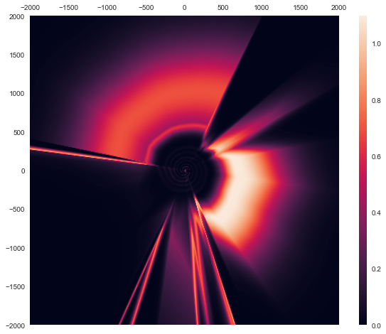
(f) EnD² Knowledge Uncertainty

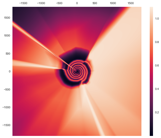
(g) EnD${}^{2}_{\tt+AUX}$ Total Uncertainty

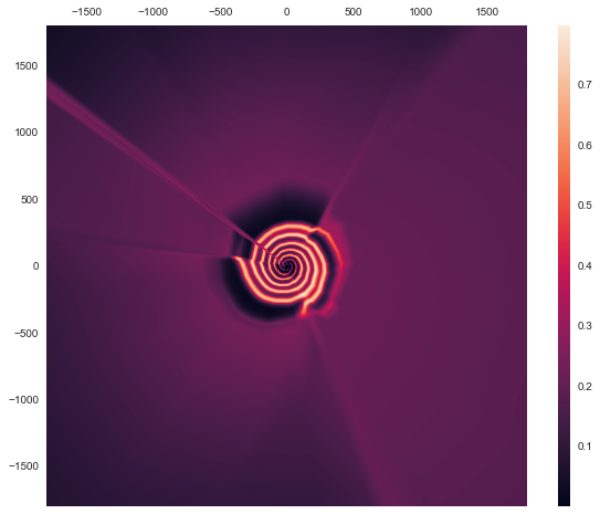
(h) EnD${}^{2}_{\tt+AUX}$ Data Uncertainty

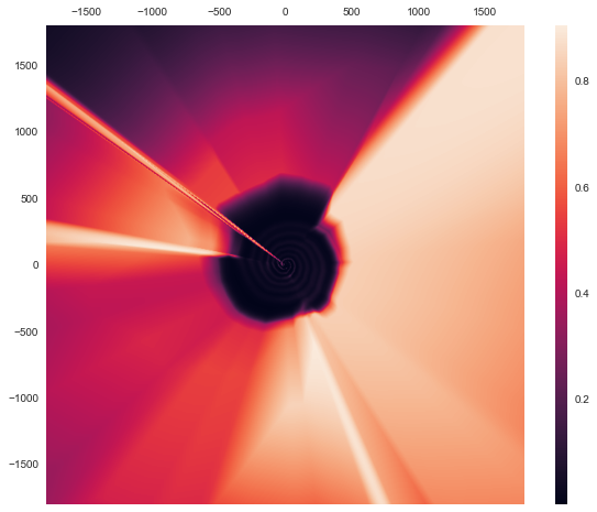
(i) EnD${}^{2}_{\tt+AUX}$ Knowledge Uncertainty

Figure 3: Comparison of measures of uncertainty derived from an Ensemble, EnD² and EnD${}^{2}_{\tt+AUX}$.

The measures of uncertainty derived form an ensemble of 100 models and from Ensemble Distribution Distillation are presented in figures 3a-c and figures 3d-f, respectively. The results show that EnD² successfully captures data uncertainty and also correctly decomposes total uncertainty into knowledge uncertainty and data uncertainty. However, it fails to appropriately capture knowledge uncertainty further away from the training region, as there are obvious dark holes in figure 3f, where the model yields low knowledge uncertainty far from the region of training data.

In order to overcome these issues, a thick ring of inputs far from the training data was sampled as depicted in figure 2b. The predictions of the ensemble were obtained for these input points and used as additional auxiliary training data $\mathcal{D}_{\tt AUX}$. Table 2 shows how using the auxiliary training data affects the performance of the Ensemble Distillation and Ensemble Distribution Distillation. There is a minor drop in performance of both distillation approaches. However, the overall level of performance is not compromised and is still higher than the average performance of each individual DNN model. The behaviour of measures of uncertainty derived from Ensemble Distribution Distillation with auxiliary training data (EnD${}^{2}_{\tt+AUX}$) is shown in figures 3g-i. These results show that successful Ensemble Distribution Distillation of the out-of-distribution behaviour of an ensemble based purely on observations of the in-domain behaviour is challenging and may require the use of additional training data. This is compounded by the fact that the diversity of an ensemble on training data that the model has seen is typically smaller than on a heldout test-set.

Table 2: Classification Performance (% Error) on $\mathcal{D}_{test}$, trained on either $\mathcal{D}_{trn}$ or $\mathcal{D}_{trn}+\mathcal{D}_{\tt AUX}$. All datasets are of size 1000. Data for an ensemble of a 100 models.

Distillation Data	Individual	Ensemble	EnD	EnD2
$\mathcal{D}_{\tt trn}$	13.21	12.37	12.39	12.47
$\mathcal{D}_{\tt trn}$ + $\mathcal{D}_{\tt AUX}$			12.41	12.50

5 Experiments on Image Data

Having confirmed the properties of EnD² on an artificial dataset, we now investigate Ensemble Distribution Distillation on the CIFAR-10 (C10), CIFAR-100 (C100) and TinyImageNet (TIM) (Krizhevsky, 2009; CS231N, 2017) datasets. Similarly to section 4, an ensemble of a 100 models is constructed by training NNs on C10/100/TIM data from different random initializations. The transfer dataset is constructed from C10/100/TIM inputs and ensemble logits to allow for temperature annealing during training, which we found to be essential to getting EnD² to train well. In addition, we also consider Ensemble Distillation and Ensemble Distribution Distillation on a transfer set that contains both the original C10/C100/TIM training data and auxiliary (AUX) data taken from the other dataset, termed EnD_+AUX and EnD${}^{2}_{\tt+AUX}$ respectively. It is important to note that the auxiliary data has been treated in the same way as main data during construction of the transfer set and distillation. This offers an advantage over traditional Prior Network training (Malinin & Gales, 2018; 2019), where the knowledge of which examples are in-domain and out-of-distribution is required a-priori. In this work we also make a comparison with Prior Networks trained via reverse KL-divergence (Malinin & Gales, 2019), where the Prior Networks (PN) are trained on the same datasets, both main and auxiliary, as the EnD_+AUX and EnD${}^{2}_{+AUX}$ models. Note, that for Ensemble Distribution Distillation, models can be distribution-distilled using any (potentially unlabeled) auxiliary data on which ensemble predictions can be obtained. Further note that in these experiments we explicitly chose to use the simpler VGG-16 (Simonyan & Zisserman, 2015) architecture rather than more modern architectures like ResNet (He et al., 2016) as the goal of this work is to analyse the properties of Ensemble Distribution Distillation in a clean and simple configuration. The datasets and training configurations for all models are detailed in appendix A.

Table 3: Mean Classification Error, % PRR , test-set negative log-likelihood (NLL) and expected calibration error (ECE) on C10/C100/TIM across three models $\pm 2\sigma$.

DSET CRIT. IND ENSM EnD EnD² EnD_+AUX EnD${}^{2}_{\tt+AUX}$ PN_+AUX C10 ERR 8.0 $\pm 0.4$ 6.2 $\pm$ NA 6.7 $\pm 0.3$ 7.3 $\pm 0.2$ 6.7 $\pm 0.2$ 6.9 $\pm 0.2$ 7.5 $\pm 0.3$ PRR 84.6 $\pm 1.2$ 86.8 $\pm$ NA 84.8 $\pm 0.8$ 85.3 $\pm 1.1$ 85.1 $\pm 0.1$ 85.7 $\pm 0.3$ 82.0 $\pm 1.4$ ECE 2.2 $\pm 0.4$ 1.3 $\pm$ NA 2.6 $\pm 0.2$ 1.0 $\pm 0.2$ 2.6 $\pm 0.6$ 2.2 $\pm 0.4$ 12.0 $\pm 0.7$ NLL 0.25 $\pm 0.01$ 0.19 $\pm$ NA 0.22 $\pm 0.01$ 0.25 $\pm 0.01$ 0.22 $\pm 0.01$ 0.24 $\pm 0.00$ 0.38 $\pm 0.01$ C100 ERR 30.4 $\pm 0.3$ 26.3 $\pm$ NA 28.0 $\pm 0.4$ 27.9 $\pm 0.3$ 28.2 $\pm 0.3$ 28.0 $\pm 0.5$ 28.0 $\pm 0.7$ PRR 72.5 $\pm 1.0$ 75.0 $\pm$ NA 73.1 $\pm 0.5$ 73.7 $\pm 0.7$ 74.0 $\pm 0.3$ 74.0 $\pm 0.2$ 63.7 $\pm 0.8$ ECE 9.3 $\pm 0.8$ 1.2 $\pm$ NA 8.2 $\pm 0.3$ 4.9 $\pm 0.5$ 1.9 $\pm 0.3$ 5.6 $\pm 0.5$ 37.9 $\pm 0.4$ NLL 1.16 $\pm 0.03$ 0.88 $\pm$ NA 1.06 $\pm 0.01$ 1.14 $\pm 0.01$ 0.98 $\pm 0.00$ 1.14 $\pm 0.01$ 1.87 $\pm 0.03$ TIM ERR 41.8 $\pm 0.6$ 36.6 $\pm$NA 38.3 $\pm 0.2$ 37.6 $\pm 0.2$ 38.5 $\pm 0.3$ 37.3 $\pm 0.5$ 40.0 $\pm 0.6$ PRR 70.8 $\pm 1.1$ 73.8 $\pm$ NA 72.2 $\pm 0.2$ 73.1 $\pm 0.1$ 72.6 $\pm 1.3$ 72.7 $\pm 1.1$ 62.3 $\pm 0.6$ ECE 18.3 $\pm 0.8$ 3.8 $\pm$ NA 14.8 $\pm 0.4$ 7.2 $\pm 0.4$ 14.9 $\pm 0.3$ 7.2 $\pm 0.2$ 39.1 $\pm 1.0$ NLL 2.15 $\pm 0.05$ 1.51 $\pm$ NA 1.77 $\pm 0.01$ 1.83 $\pm 0.02$ 1.78 $\pm 0.01$ 1.84 $\pm 0.02$ 2.61 $\pm 0.01$

Firstly, we investigate the ability of a single model to retain the ensemble’s classification and prediction-rejection (misclassification detection) performance after either Ensemble Distillation (EnD) or Ensemble Distribution Distillation (EnD²), with results presented in table 3 in terms of error rate and prediction rejection ratio (PRR), respectively. A higher PRR indicates that the model is able to better detect and reject incorrect predictions based on measures of uncertainty. This metric is detailed in appendix B. Note that for prediction rejection we used the confidence of the max class, which also is a measure of total uncertainty, like entropy, but is more sensitive to the prediction (Malinin & Gales, 2018).

Table 3 shows that both EnD and EnD² are able to retain both the improved classification and prediction-rejection performance of the ensemble relative to individual models trained with maximum likelihood on all datasets, both with and without auxiliary training data. Note, that on C100 and TIM, EnD² yields marginally better classification performance than EnD. Furthermore, EnD² also either consistently outperforms or matches EnD in terms of PRR on all datasets, both with and without auxiliary training data. This suggests that EnD² is able to yield benefits on top of standard Ensemble Distillation due to retaining information about the diversity of the ensemble. In comparison, a Prior Network, while yielding a classification performance between that on an individual model and EnD${}^{2}_{+AUX}$, performs consistently worse than all models in terms of PRR and for all datasets. This is likely because of the inappropriate choice of auxiliary training data and auxiliary loss weight (Malinin & Gales, 2019) for this task.

Secondly, it is known that ensembles yield improvements in the calibration of a model’s predictions (Lakshminarayanan et al., 2017; Ovadia et al., 2019). Thus, it is interesting to see whether EnD and EnD² models retain these improvements in terms of test-set negative log-likelihood (NLL) and expected calibration error (ECE). Note that calibration assesses uncertainty quality on a per-dataset, rather than per-prediction, level. From table 3 we can see that both Ensemble Distillation and Ensemble Distribution Distillation seem to give similarly minor gains in NLL over a single model. However, EnD seems to have marginally better NLL performance, while EnD² tends to yield better calibration performance. There are seemingly limited gains in ECE and NLL when using auxiliary data during distillation for EnD², and sometimes even a degradation in NLL and ECE. This may be due to the Dirichlet output distribution attempting to capture non-Dirichlet-distributed ensemble predictions (especially on auxiliary data) and over-estimating the support, and thereby failing to fully reproduce the calibration of the original ensemble. Furthermore, metrics like ECE and NLL are evaluated on in-domain data, which would explain the lack of improvement from distilling ensemble behaviour on auxiliary data. However, all distillation models are (almost) always calibrated as better than individual models. At the same time, the Prior Network models yield significantly worse calibration performance in terms of NLL and ECE than all other models. For the CIFAR-100 and TIM datasets this may be due to the target being a flat Dirichlet distribution for the auxiliary data (CIFAR-10), which drives the model to be very under-confident.

Table 4: OOD detection performance (mean % AUC-ROC $\pm 2\sigma$) for C10/C100/TIM models using measures of total (T.Unc) and knowledge (K.Unc) uncertainty.

Train. OOD Unc. Individual Ensemble EnD EnD² EnD_+AUX EnD${}^{2}_{\tt+AUX}$ PN_+AUX Data Data C10 LSUN T.Unc 91.3 $\pm 1.3$ 94.5 $\pm$N/A 89.0 $\pm 1.3$ 91.5 $\pm 0.8$ 88.6 $\pm 1.1$ 94.4 $\pm 0.7$ 95.7 $\pm 0.9$ K.Unc - 94.4 $\pm$N/A - 92.2 $\pm 0.7$ - 93.8 $\pm 0.7$ 95.8 $\pm 0.8$ TIM T.Unc 88.9 $\pm 1.6$ 91.8 $\pm$N/A 86.9 $\pm 1.2$ 88.6 $\pm 1.5$ 86.5 $\pm 1.6$ 91.3 $\pm 0.8$ 95.7 $\pm 0.7$ K.Unc - 91.4 $\pm$N/A - 88.8 $\pm 1.6$ - 90.6 $\pm 0.7$ 95.8 $\pm 0.7$ C100 LSUN T.Unc 75.6 $\pm 1.1$ 82.4 $\pm$N/A 73.8 $\pm 0.6$ 80.6 $\pm 1.1$ 80.6 $\pm 0.6$ 83.6 $\pm 0.5$ 74.8 $\pm 1.7$ K.Unc - 88.4 $\pm$N/A - 83.8 $\pm 0.9$ - 86.5 $\pm 0.5$ 73.8 $\pm 2.2$ TIM T.Unc 70.5 $\pm 1.5$ 76.6 $\pm$N/A 68.5 $\pm 1.2$ 74.4 $\pm 1.5$ 74.2 $\pm 0.8$ 77.7 $\pm 0.9$ 73.4 $\pm 2.9$ K.Unc - 81.7 $\pm$N/A - 77.2 $\pm 1.5$ - 80.5 $\pm 1.1$ 72.7 $\pm 3.3$ TIM LSUN T.Unc 67.5 $\pm 1.3$ 69.7 $\pm$N/A 68.7 $\pm 0.2$ 69.6 $\pm 1.4$ 68.8 $\pm 0.2$ 69.2 $\pm 0.7$ 63.7 $\pm 0.1$ K.Unc - 69.3 $\pm$N/A - 70.4 $\pm 1.3$ - 70.3 $\pm 0.4$ 59.5 $\pm 1.9$ C100 T.Unc 71.7 $\pm 2.5$ 75.2 $\pm$N/A 73.1 $\pm 0.7$ 74.8 $\pm 0.3$ 73.1 $\pm 0.3$ 74.1 $\pm 1.3$ 100.0 $\pm 0.0$ K.Unc - 78.8 $\pm$N/A - 76.7 $\pm 0.5$ - 75.3 $\pm 0.7$ 100.0 $\pm 0.0$

Thirdly, Ensemble Distribution Distillation is investigated on the task of out-of-domain (OOD) input detection (Hendrycks & Gimpel, 2016), where measures of uncertainty are used to classify inputs as either in-domain (ID) or OOD. The ID examples are the test set of C10/100/TIM, and the test OOD examples are chosen to be the test sets of LSUN (Yu et al., 2015), C100 or TIM, such that the test OOD data is never seen by the model during training. Table 4 shows that the measures of uncertainty derived from the ensemble outperform those from a single neural network. Curiously, standard ensemble distillation (EnD) clearly fails to capture those gains on C10 and TIM, both with and without auxiliary training data, but does reach a comparable level of performance to the ensemble on C100. Curiously, EnD_+AUX performs worse than the individual models on C10. This is in contrast to results from (Englesson & Azizpour, 2019; Li & Hoiem, 2019), but the setups, datasets and evaluation considered there are very different to ours. On the other hand, Ensemble Distribution Distillation is generally able to reproduce the OOD detection performance of the ensemble. When auxiliary training data is used, EnD² is able to perform on par with the ensemble, indicating that it has successfully learned how the distribution of the ensemble behaves on unfamiliar data. These results suggest that not only is EnD² able to preserve information about the diversity of an ensemble, unlike standard EnD, but that this information is important to achieving good OOD detection performance. Notably, on the CIFAR-10 dataset PNs yield the best performance. However, due to generally inappropriate choice of OOD (auxiliary) training data, PNs show inferior (with one exception) OOD detection performance on CIFAR-100 and TIM.

Curiously, the ensemble sometimes displays better OOD detection performance using measures of total uncertainty. This is partly a property of the in-domain dataset - if it contains a small amount of data uncertainty, then OOD detection performance using total uncertainty and knowledge uncertainty should be almost the same (Malinin & Gales, 2018; Malinin, 2019). Unlike the toy dataset considered in the previous section, where significant data uncertainty was added, the image datasets considered here do have a low degree of data uncertainty. It is important to note that on more challenging tasks, which naturally exhibit a higher level of data uncertainty, we would expect that the decomposition would be more beneficial. Additionally, it is also possible that if different architectures, training regimes and ensembling techniques are considered, an ensemble with a better estimate of knowledge uncertainty can be obtained. Despite the behaviour of the ensemble, EnD², especially with auxiliary training data, tends to have better OOD detection performance using measures of knowledge uncertainty. This may be due to the use of a Dirichlet output distribution, which may not be able to fully capture the details of the ensemble’s behaviour. Furthermore, as EnD² is (implicitly) trained by minimizing the forward KL-divergence, which is zero-avoiding (Murphy, 2012), it is likely that the distribution learned by the model is ‘wider’ than the empirical distribution. This effect is explored in the next subsection and in appendix C.

5.1 Appropriateness of Dirichlet distribution

Throughout this work, a Prior Network that parametrizes a Dirichlet was used for distribution-distilling ensembles of models. However, the output distributions of an ensemble for the same input are not necessarily Dirichlet-distributed, especially in regions where the ensemble is diverse. In the previous section we saw that EnD² models tend to have higher NLL than EnD models, and while EnD² achieves good OOD detection performance, it doesn’t fully replicate the ensemble’s behaviour. Thus, in this section, we investigate how well a model which parameterizes a Dirichlet distribution is able to capture the exact behaviour of an ensemble of models, both in-domain and out-of-distribution.

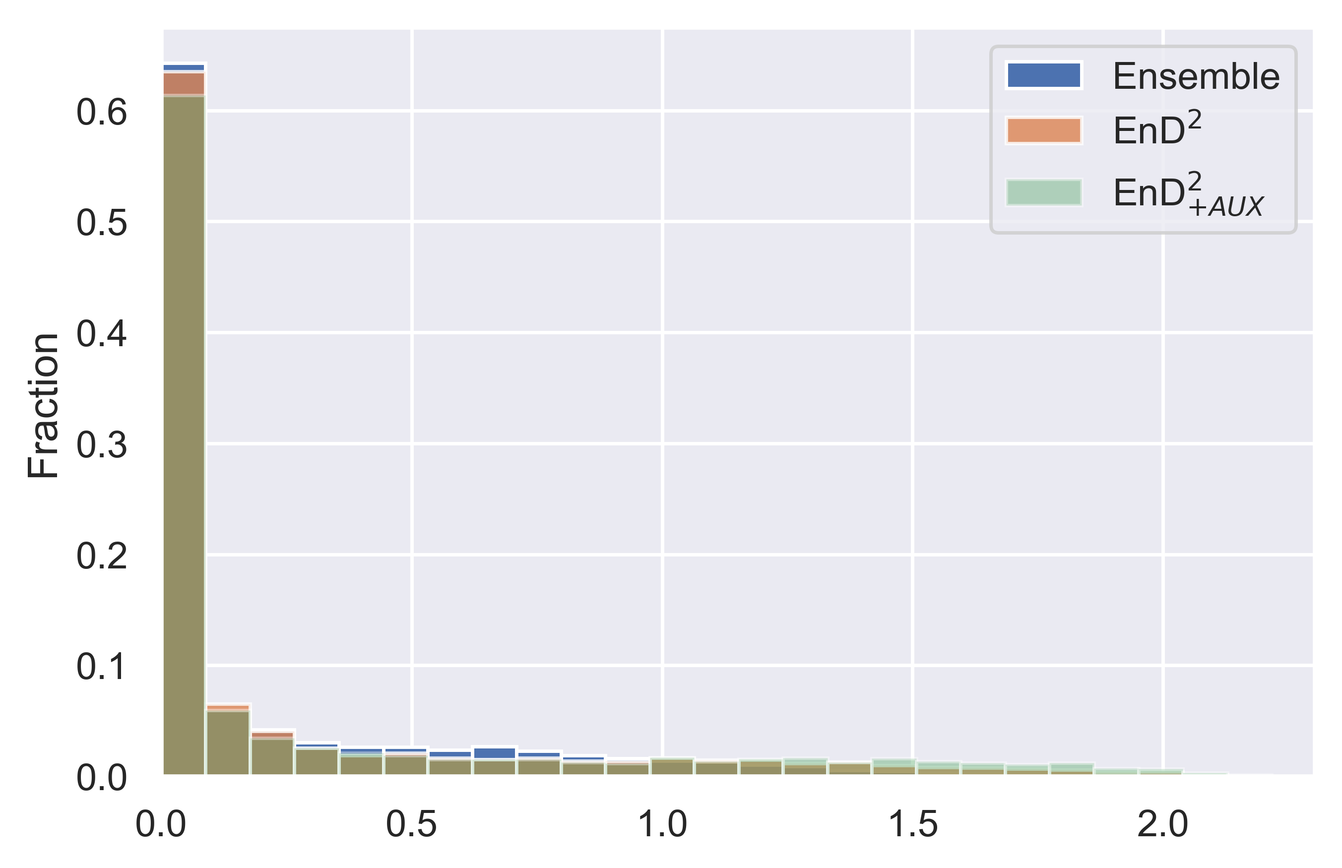
(a) Total Uncertainty - ID

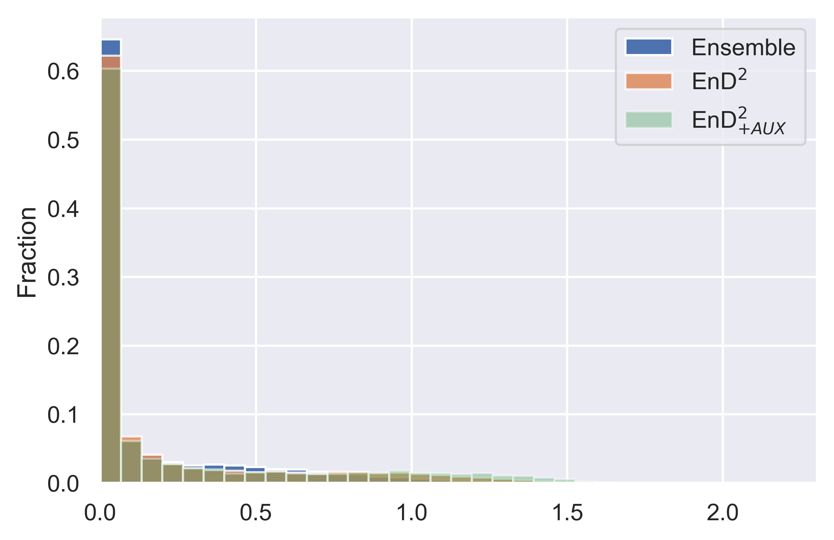
(b) Data Uncertainty - ID

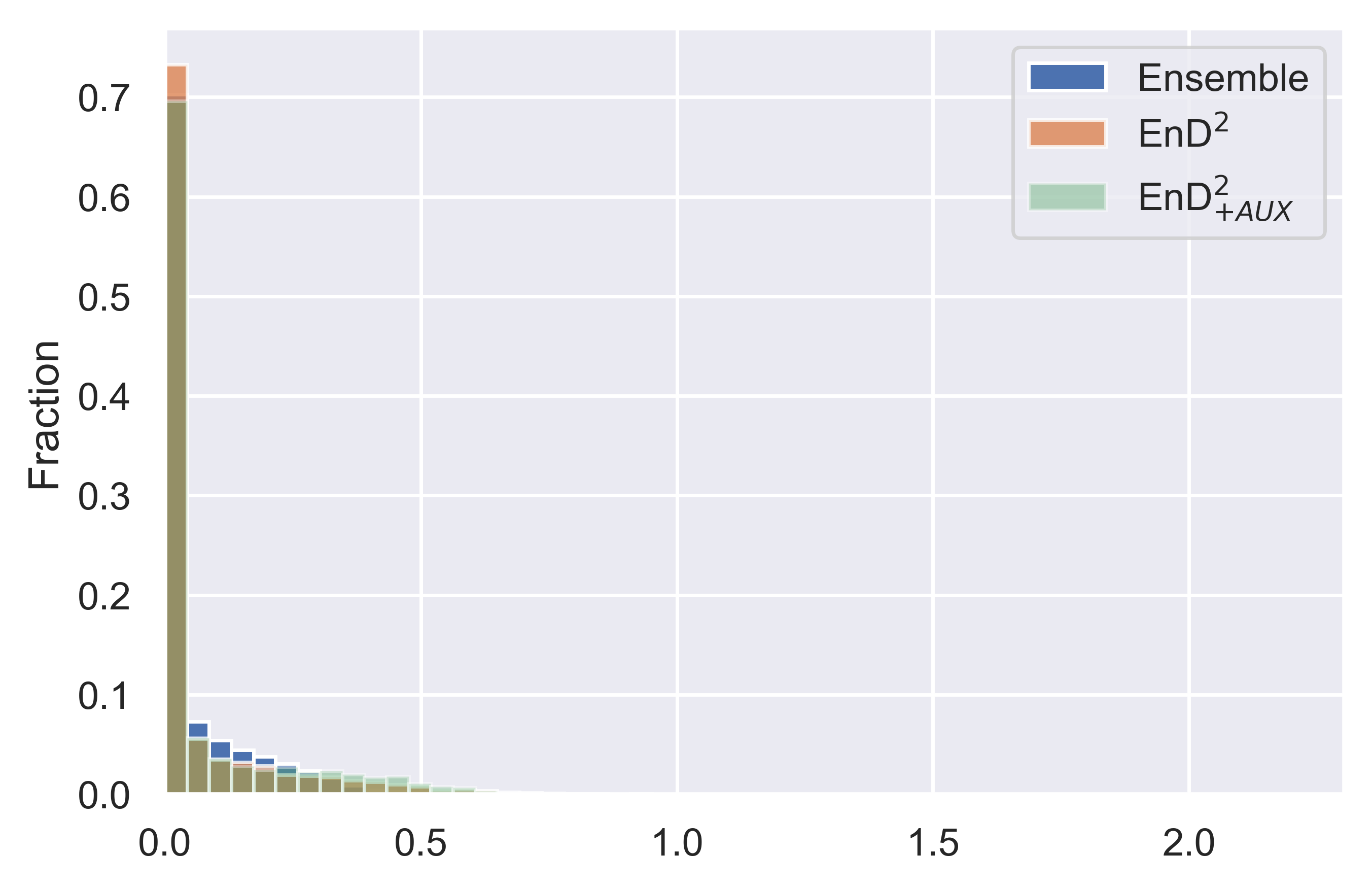
(c) Knowledge Uncertainty - ID

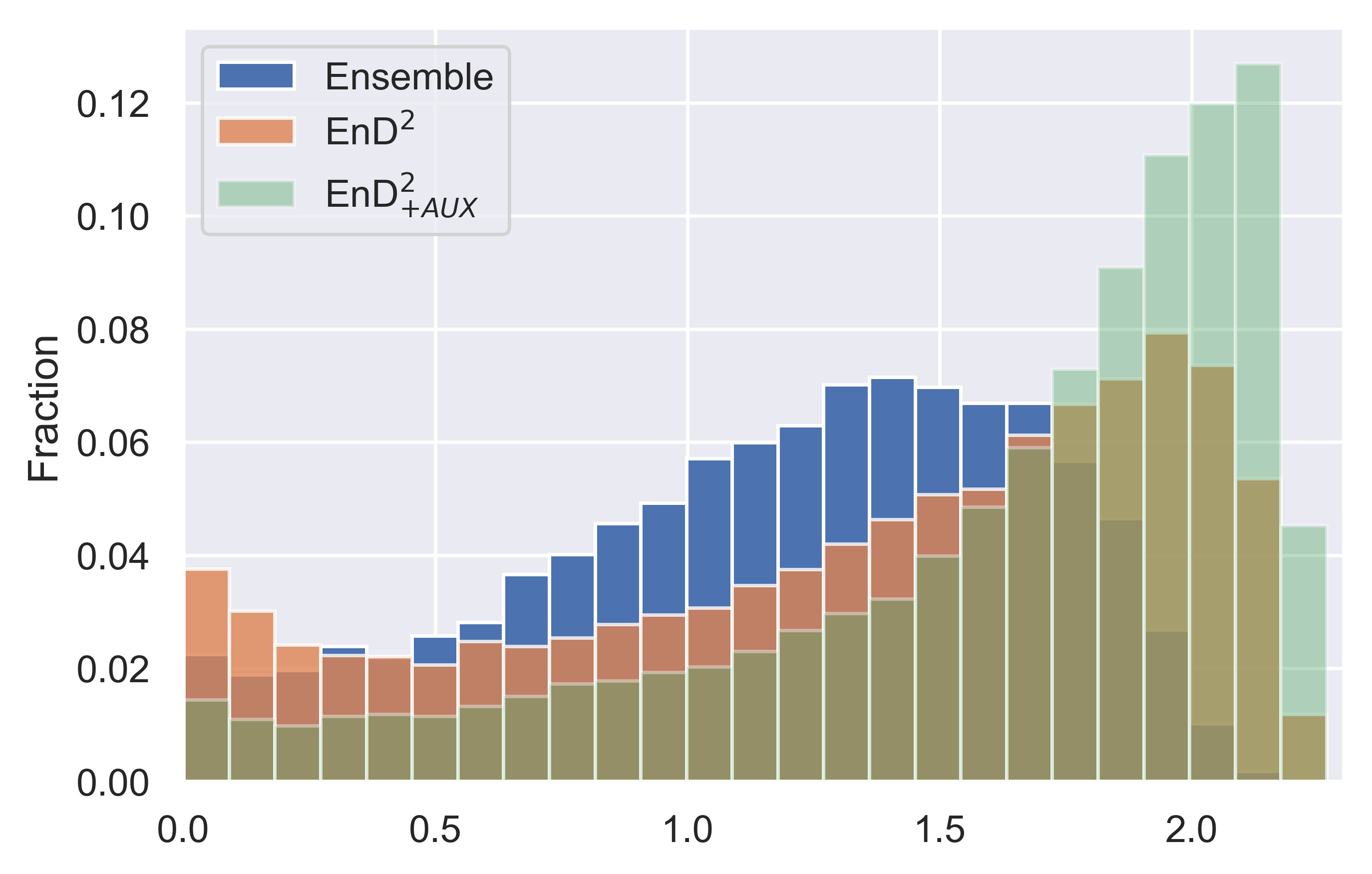
(d) Total Uncertainty - OOD

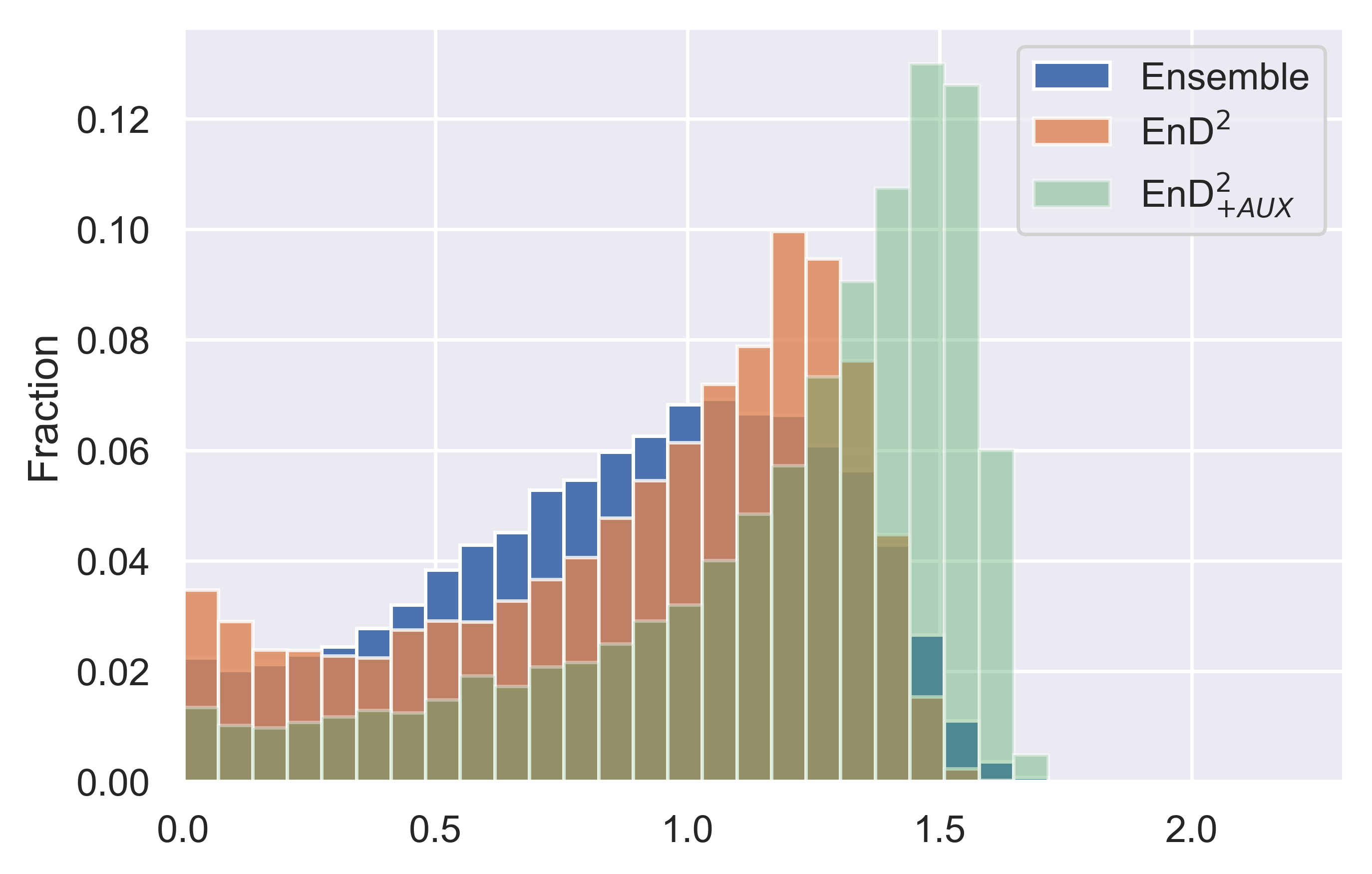
(e) Data Uncertainty - OOD

(f) Knowledge Uncertainty - OOD

Figure 4: Histograms of uncertainty of the CIFAR-10 ensemble, EnD² and EnD${}^{2}_{\tt+AUX}$ on in-domain (ID) and test out-of-domain (OOD) data.

Figure 4 shows histograms of total uncertainty, data uncertainty and total uncertainty yielded by an ensemble, EnD² and EnD${}^{2}_{\tt+AUX}$ models trained on the CIFAR-10 dataset. The top row shows the uncertainty histogram for ID data, and the bottom for test OOD data (a concatenation of LSUN and TIM). On in-domain data, EnD² is seemingly able to emulate the uncertainty metrics of the ensemble well, though does have a longer tail of high-uncertainty examples. This is expected, as on in-domain examples the ensemble will be highly concentrated around the mean. This behaviour can be adequately modelled by a Dirichlet. On the other hand, there is a noticeable mismatch between the ensemble and EnD² in the uncertainties they yield on OOD data. Here, EnD² consistently yields higher uncertainty predictions than the original ensemble. Notably, adding auxiliary training data makes the model yield even higher estimates of total uncertainty and data uncertainty. At the same time, by using auxiliary training data, the model’s distribution of knowledge uncertainty starts to look more like the ensembles, but shifted to the right (higher).

Altogether, this suggests that samples from the ensemble are diverse in a way that’s different from a Dirichlet distribution. For instance, the distribution could be multi-modal or crescent-shaped. Thus, as a consequence of this, combined with forward KL-divergence between the model and the empirical distribution of the ensemble being zero-avoiding, the model over-estimates the support of the empirical distribution, yielding an output which is both more diverse and higher entropy than the original ensemble. This does not seem to adversely impact OOD detection performance as measures of uncertainty for ID and OOD data are further spread apart and the rank ordering of ID and OOD data is either maintained or improved, which is supported by results from section 5. However, this does prevent the EnD² models from fully retaining the calibration quality of the ensemble. It is possible that the ensemble could be better modelled by a different output distribution, such as a mixture of Dirichlet distributions or a Logistic-normal distribution.

6 Conclusion

Ensemble Distillation approaches have become popular, as they allow a single model to achieve classification performance comparable to that of an ensemble at a lower computational cost. This work proposes the novel task Ensemble Distribution Distillation (EnD²) — distilling an ensemble into a single model, such that it exhibits both the improved classification performance of the ensemble and retains information about its diversity. An approach to EnD² based on using Prior Network models is considered in this work. Experiments described in sections 4 and 5 show that on both artificial data and image classification tasks it is possible to distribution distill an ensemble into a single model such that it retains the classification performance of the ensemble. Furthermore, measures of uncertainty provided by EnD² models match the behaviour of an ensemble of models on artificial data, and EnD² models are able to differentiate between different types of uncertainty. However, this may require obtaining auxiliary training data on which the ensemble is more diverse in order to allow the distribution-distilled model to learn appropriate out-of-domain behaviour. On image classification tasks measures of uncertainty derived from EnD² models allow them to outperform both single NNs and EnD models on the tasks of misclassification and out-of-distribution input detection. These results are promising, and show that Ensemble Distribution Distillation enables a single model to capture more useful properties of an ensemble than standard Ensemble Distillation. Future work should further investigate properties of temperature annealing, investigate ways to enhance the diversity of an ensemble, consider different sources of ensembles and model architectures, and examine more flexible output distributions, such as mixtures of Dirichlets. Furthermore, while this work considered Ensemble Distribution Distillation only for classification problems, it can and should also be investigated for regression tasks. Finally, it may be interesting to explore combining Ensemble Distribution Distillation with standard Prior Network training.

Appendix A Datasets, Model architecture and training

Table 5: Description of datasets used in the experiments in terms of number of images and classes.

Dataset Train Valid Test Classes CIFAR-10 50000 - 10000 10 CIFAR-100 50000 - 10000 100 TinyImagenet 100000 - 10000 200 LSUN (evaluation only) - - 10000 10

All models considered in this work were implemented in Pytorch (Paszke et al., 2017) using a variant of the VGG16 (Simonyan & Zisserman, 2015) architecture for image classification. DNN and EnD models were trained using the negative log-likelihood loss of the labels and the mean ensemble predictions respectively. EnD² models were trained using the negative log-likelihood of the ensemble’s output categorical distributions. All models were trained using the Adam (Kingma & Ba, 2015) optimizer, with a 1-cycle learning rate policy and dropout regularization. For all ensembles, models were trained using different random seed initialization, and using different seeds for shuffling the data. In addition, data augmentation was applied via random left-right flips, random shifts up to $\pm$4 pixels and random rotations by up to $\pm$ 15 degrees. Tables e 6 details the training configurations for all models. Furthermore, batch normalisation was used for both Ensemble Distillation and Ensemble Distribution Distillation, but not for Prior Networks.

Table 6: Training Configurations. $\eta_{0}$ is the initial learning rate, $T_{0}$ is the initial temperature and ’Annealing’ refers to whether a temperature annealing schedule was used. The batch size for all models was 128. Dropout rate is quoted in terms of probability of not dropping out a unit.

Training Model General Distillation Dataset $\eta_{0}$ Epochs Cycle len. Dropout $T_{0}$ Annealing AUX data CIFAR-10 DNN $10^{-3}$ 45 30 0.5 - - - EnD 90 60 0.7 $2.5$ No - EnD_+AUX 90 60 0.7 $2.5$ No CIFAR-100 EnD² 90 60 0.7 $10$ Yes - EnD${}^{2}_{\tt+AUX}$ 90 60 0.7 $10$ Yes CIFAR-100 PN $5\!\times\!10^{-4}$ 45 30 0.7 - No CIFAR-100 CIFAR-100 DNN $10^{-3}$ 100 150 0.5 - - - EnD 200 150 0.9 $2.5$ No - EnD_+AUX 200 150 0.9 $2.5$ No CIFAR-10 EnD² 200 150 0.9 $10$ Yes - EnD${}^{2}_{\tt+AUX}$ 200 150 0.9 $10$ Yes CIFAR-10 PN $5\!\times\!10^{-4}$ 100 70 0.7 - No CIFAR-10 TinyImageNet DNN $10^{-3}$ 100 70 0.5 - - - EnD $5\!\times\!10^{-4}$ 200 150 0.8 $2.5$ No - EnD_+AUX $5\!\times\!10^{-4}$ 200 150 0.8 $2.5$ No CIFAR-10 EnD² $5\!\times\!10^{-4}$ 200 150 0.8 $10$ Yes - EnD${}^{2}_{\tt+AUX}$ $5\!\times\!10^{-4}$ 200 150 0.8 $10$ Yes CIFAR-10 PN $5\!\times\!10^{-4}$ 100 70 0.7 - No CIFAR-10

To create the transfer set $\mathcal{D}_{\tt ens}$, ensembles were evaluated on the unaugmented CIFAR-10 and CIFAR-100 training examples. During distillation (both EnD and EnD²), models were trained on the augmented examples with the ensemble predictions on the corresponding unaugmented inputs.

A.1 Numerical issues with maximum likelihood Dirichlet training

As shown in equation 8, ensemble distribution distillation into a prior network via likelihood maximisation is equivalent to minimising the loss function:

$$\begin{split}\mathcal{L}(\bm{\phi},\mathcal{D}_{\tt ens})=&\ -\frac{1}{N}\sum_{i=1}^{N}\Big{[}\ln\Gamma(\hat{\alpha}_{0}^{(i)})-\sum_{c=1}^{K}\ln\Gamma(\hat{\alpha}_{c}^{(i)})+\frac{1}{M}\sum_{m=1}^{M}\sum_{c=1}^{K}(\hat{\alpha}_{c}^{(i)}-1)\ln\pi_{c}^{(im)}\Big{]}\end{split}$$ (11)

If, due to numerical precision of the implementation, one of the ensemble member sample terms $\pi_{c}^{(im)}$ gets rounded to $0.0$, the log term $\ln\pi_{c}^{(im)}$ in the above equation cannot be computed. To avoid this, we apply a small amount of central smoothing to the ensemble predictions:

$$\begin{split}\pi_{c,smoothed}^{(im)}=(1-\gamma)\pi_{c}^{(im)}+\gamma\frac{1}{K}\end{split}$$ (12)

Where the smoothing parameter parameter $\gamma$ has been set to $1\text{\times}{10}^{-4}$ for all EnD² experiments. Note that after applying central smoothing, each ensemble member’s predictions still sum up to $1.0$.

A.2 Temperature Annealing Schedule

A fixed temperature of $2.5$ was used for Ensemble Distillation as recommended in (Hinton et al., 2015), and was found to yield the best classification performance out of $\{1,2.5,5,10\}$. Temperature annealing resulted in worse classification performance for Ensemble Distillation, and hence was not used in the experiments. For the temperature annealing schedule, the temperature was kept fixed to initial temperature $T_{0}$ for the first half-cycle. For the second half-cycle we linearly decayed the initial temperature $T_{0}$ down to $1.0$. Then, the temperature was kept constant at $1.0$ for the remainder of the epochs. For Ensemble Distribution Distillation, we found that an initial temperature of $10$ performed best out of $\{5,10,20\}$. The choice of the particular annealing schedule used has not been tested extensively, and it is possible that other schedules that lead to faster training exist. However, we must point out that it was necessary to use temperature scaling to train models on the CIFAR-10, CIFAR-100 and TinyImageNet datasets.

Appendix B Assessing misclassification detection performance

In this work measures of uncertainty are used for two practical applications of uncertainty - misclassification detection and out-of-distribution sample detection. Both can be seen as an outlier detection task based on measures of uncertainty, where misclassifications are one form of outlier and out-of-distribution inputs are another form of outlier. These tasks can be formulated as threshold-based binary classification (Hendrycks & Gimpel, 2016). Here, a detector $\mathcal{I}_{T}(\bm{x})$ assigns the label 1 (uncertain prediction) if an uncertainty measure $\mathcal{H}(\bm{x})$ is above a threshold $T$, and label 0 (confident prediction) otherwise. This uncertainty measure can be any of the measures discussed in sections 2 and 3.

$$\mathcal{I}_{T}(\bm{x})=\ \begin{cases}1,\ \mathcal{H}(\bm{x})>T\\ 0,\ \mathcal{H}(\bm{x})\leq T\\ \end{cases}$$ (13)

Given a set of true positive examples $\mathcal{D}_{\tt p}=\{\bm{x}_{p}^{(i)}\}_{i=1}^{N_{p}}$ and a set of true negative examples $\mathcal{D}_{\tt n}=\{\bm{x}_{n}^{(j)}\}_{j=1}^{N_{n}}$ the performance of such a detection scheme can be evaluated at a particular threshold value $T$ using the true positive rate $t_{p}(T)$ and the false positive rate $f_{p}(T)$:

$$t_{p}(T)=\ \frac{1}{N_{p}}\sum_{i=1}^{N_{p}}\mathcal{I}_{T}(\bm{x}_{p}^{(i)})\quad \quad f_{p}(T)=\ \frac{1}{N_{n}}\sum_{j=1}^{N_{n}}\mathcal{I}_{T}(\bm{x}_{n}^{(j)})$$ (14)

The range of trade-offs between the true positive and the false positive rates can be visualized using a Receiver-Operating-Characteristic (ROC) and the quality of the possible trade-offs can be summarized using the area under the ROC curve (AUROC) (Murphy, 2012). If there are significantly more negatives than positives, however, this measure will over-estimate the performance of the model and yield a high AUROC value (Murphy, 2012). In this situation it is better to calculate the precision and recall of this detection scheme at every threshold value and plot them against each other on a Precision-Recall (PR) curve (Murphy, 2012). The recall $R(T)$ is equal to the true positive rate $t_{p}(T)$, while precision measures the number of true positives among all samples labelled as positive:

$$P(T)=\ \frac{\sum_{i=1}^{N_{p}}\mathcal{I}_{T}(\bm{x}_{p}^{(i)})}{\sum_{i=1}^{N_{p}}\mathcal{I}_{T}(\bm{x}_{p}^{(i)})+\sum_{j=1}^{N_{n}}\mathcal{I}_{T}(\bm{x}_{n}^{(j)})}\quad \quad R(T)=\ \frac{1}{{N_{p}}}\sum_{i=1}^{N_{p}}\mathcal{I}_{T}(\bm{x}_{p}^{(i)})$$ (15)

The quality of the trade-offs can again be summarized via the area under the PR curve (AUPR). For both the ROC and the PR curves an ideal detection scheme will achieve an AUC of 100%. A completely random detection scheme will have an AUROC of 50% and the AUPR will be the ratio of the number of positive examples to the total size of the dataset (positive and negative) (Murphy, 2012). Thus, the recall is given by the error rate of the classifier. This makes it difficult to compare different models with different base error rates, as AUPR can increase both due to better misclassification detection and worse error rates.

Below we provide AUPR numbers for all models and datasets in order to illustrate how it can challenging to compare models using this metric. The difference in AUPR between models within a dataset is typically similar to the difference in classification performance. Thus, it is challenging to assesses whether a higher AUPR is due to better misclassification detection or higher error rate. Additionally, this table illustrate that confidence of the prediction is a better measure of uncertainty than entropy for this task. At the same, knowledge uncertainty yield much worse misclassification detection performance. These results are consistent with (Malinin & Gales, 2018; Malinin, 2019).

Table 7: Mean Misclassification detection using AUPR using different measures of uncertainty for C10/C100/TIM across three models $\pm 2\sigma$.

Dataset Model Total Uncertainty Knowledge % Error Confidence Entropy Uncertainty C10 DNN 48.2 $\pm 2.7$ 47.0 $\pm 3.4$ - 8.0 $\pm 0.4$ ENS 43.9 $\pm$ NA 41.1 $\pm$ NA 36.8 $\pm$ NA 6.2 $\pm$ NA EnD 44.6 $\pm 3.3$ 44.1 $\pm 3.9$ 37.6 $\pm 2.7$ 6.7 $\pm 0.3$ EnD² 46.8 $\pm 1.2$ 46.1 $\pm 1.0$ 43.6 $\pm 0.9$ 7.3 $\pm 0.2$ EnD_+AUX 44.5 $\pm 2.0$ 43.8 $\pm 1.7$ 37.7 $\pm 1.1$ 6.7 $\pm 0.2$ EnD${}^{2}_{+AUX}$ 46.5 $\pm 3.9$ 44.3 $\pm 3.5$ 39.4 $\pm 3.0$ 6.9 $\pm 0.2$ PN-RKL 40.5 $\pm 3.0$ 38.5 $\pm 2.7$ 35.0 $\pm 2.3$ 7.5 $\pm 0.3$ C100 DNN 69.8 $\pm 1.5$ 69.4 $\pm 1.4$ - 30.4 $\pm 0.3$ ENS 67.2 $\pm$ NA 64.0 $\pm$ NA 57.6 $\pm$ NA 26.3 $\pm$ NA EnD 68.1 $\pm 0.8$ 67.6 $\pm 1.1$ 62.2 $\pm 1.8$ 28.0 $\pm 0.4$ EnD² 68.3 $\pm 1.6$ 66.8 $\pm 1.5$ 63.4 $\pm 1.2$ 27.9 $\pm 0.3$ EnD_+AUX 69.3 $\pm 0.3$ 66.9 $\pm 0.2$ 58.0 $\pm 0.2$ 28.2 $\pm 0.3$ EnD${}^{2}_{+AUX}$ 68.9 $\pm 0.4$ 66.7 $\pm 0.2$ 62.0 $\pm 1.0$ 28.0 $\pm 0.5$ PN-RKL 60.1 $\pm 1.8$ 58.0 $\pm 1.8$ 52.8 $\pm 2.2$ 28.0 $\pm 0.7$ TIM DNN 77.9 $\pm 1.3$ 78.3 $\pm 1.2$ - 41.8 $\pm 0.6$ ENS 76.5 $\pm$ NA 74.8 $\pm$ NA 71.8 $\pm$ NA 36.6 $\pm$NA EnD 76.6 $\pm 0.5$ 77.3 $\pm 0.8$ 70.5 $\pm 1.1$ 38.3 $\pm 0.2$ EnD² 77.0 $\pm 1.0$ 76.4 $\pm 0.9$ 74.8 $\pm 1.3$ 37.6 $\pm 0.2$ EnD_+AUX 76.9 $\pm 1.8$ 77.1 $\pm 2.1$ 69.9 $\pm 1.2$ 38.5 $\pm 0.3$ EnD${}^{2}_{+AUX}$ 76.4 $\pm 1.7$ 75.8 $\pm 1.6$ 74.3 $\pm 2.1$ 37.3 $\pm 0.5$ PN-RKL 73.0 $\pm 1.2$ 71.1 $\pm 1.1$ 60.7 $\pm 1.3$ 40.0 $\pm 0.6$

In this work we consider an alternative to using AUPR to assess misclassification detection performance proposed in (Malinin, 2019). Consider the task of misclassification detection - ideally we would like to detect all of the inputs which the model has misclassified based on a measure of uncertainty. Then, the model can either choose to not provide any prediction for these inputs, or they can be passed over or ‘rejected’ to an oracle (ie: human) to obtain the correct prediction. The latter process can be visualized using a rejection curve depicted in figure 5, where the predictions of the model are replaced with predictions provided by an oracle in some particular order based on estimates of uncertainty. If the estimates of uncertainty are ‘useless’, then, in expectation, the rejection curve would be a straight line from base error rate to the lower right corner. However, if the estimates of uncertainty are ‘perfect’ and always bigger for a misclassification than for a correct classification, then they would produce the ‘oracle’ rejection curve. The ‘oracle’ curve will go down linearly to $0\%$ classification error at the percentage of rejected examples equal to the number of misclassifications. A rejection curve produced by estimates of uncertainty which are not perfect, but still informative, will sit between the ‘random’ and ‘oracle’ curves.

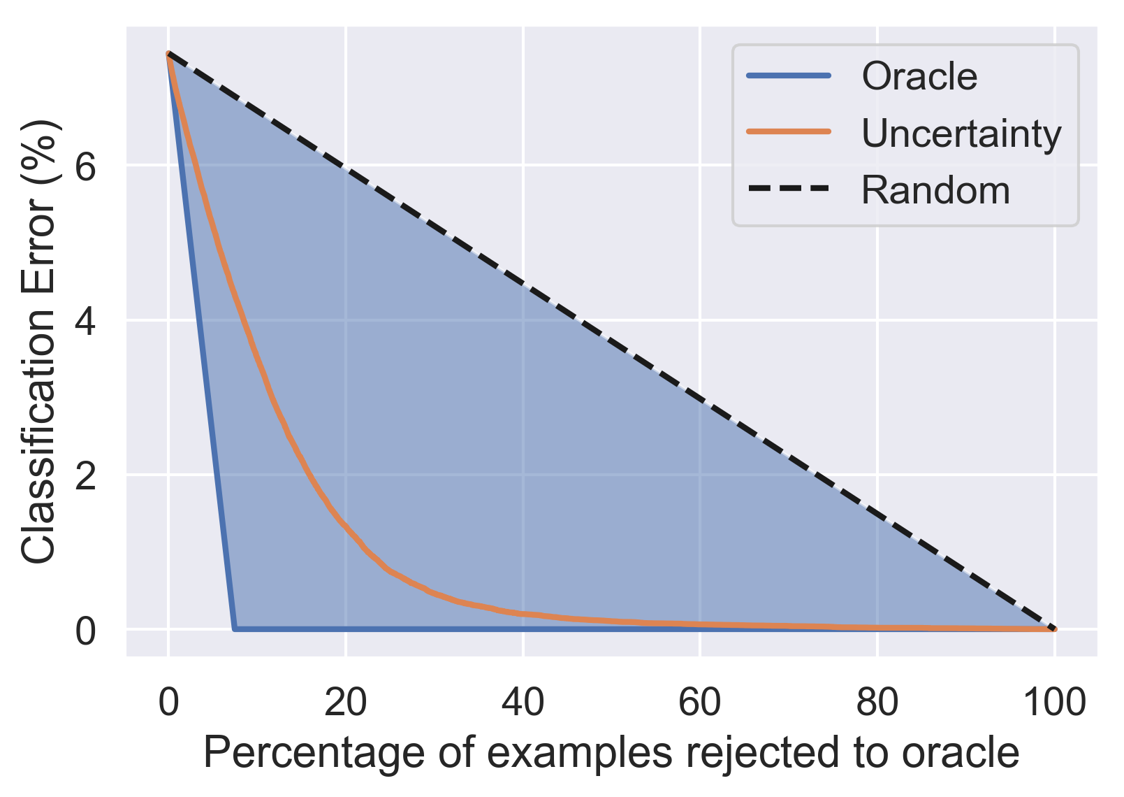
(a) Shaded area is $AR_{\tt orc}$.

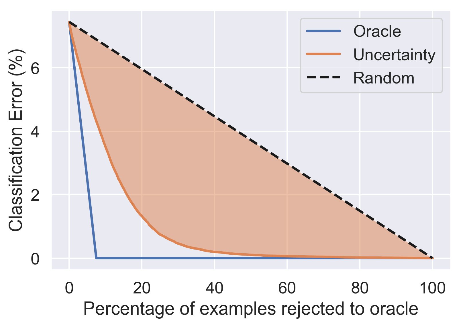
(b) Shaded area is $AR_{\tt uns}$.

Figure 5: Prediction Rejection Curves

The quality of the rejection curve can be assessed by considering the ratio of the area between the ‘uncertainty’ and ‘random’ curves $AR_{\tt uns}$ (orange in figure 5) and the area between the ‘oracle’ and ‘random’ curves $AR_{\tt orc}$ (blue in figure 5). This yields the prediction rejection area ratio $PRR$:

$$PRR=\frac{AR_{\tt uns}}{AR_{\tt orc}}$$ (16)

A rejection area ratio of 1.0 indicates optimal rejection, a ratio of 0.0 indicates ‘random’ rejection. A negative rejection ratio indicates that the estimates of uncertainty are ‘perverse’ - they are higher for accurate predictions than for misclassifications. An important property of this performance metric is that it is independent of classification performance, unlike AUPR, and thus it is possible to compare models with different base error rates. Note, that similar approaches to assessing misclassification detection were considered in (Lakshminarayanan et al., 2017; Malinin et al., 2017)

Appendix C Appropriateness of Dirichlet distribution

Section 5.1 explored the behaviour of measures of uncertainty predicted by models trained on the CIFAR-10 dataset. In this appendix we provide the same for models trained on CIFAR-100 and TinyImageNet. In general, the trends detailed in section 5.1 hold for these datasets as well - EnD² consistently yield higher uncertainties than the original ensemble, likely as a consequence of the limitations of the Dirichlet distribution.

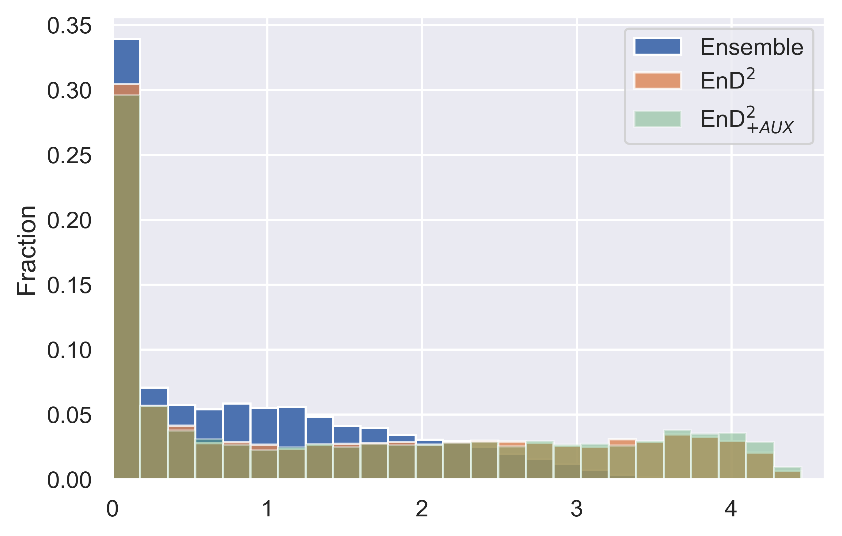
(a) C100 Total Uncert. - ID

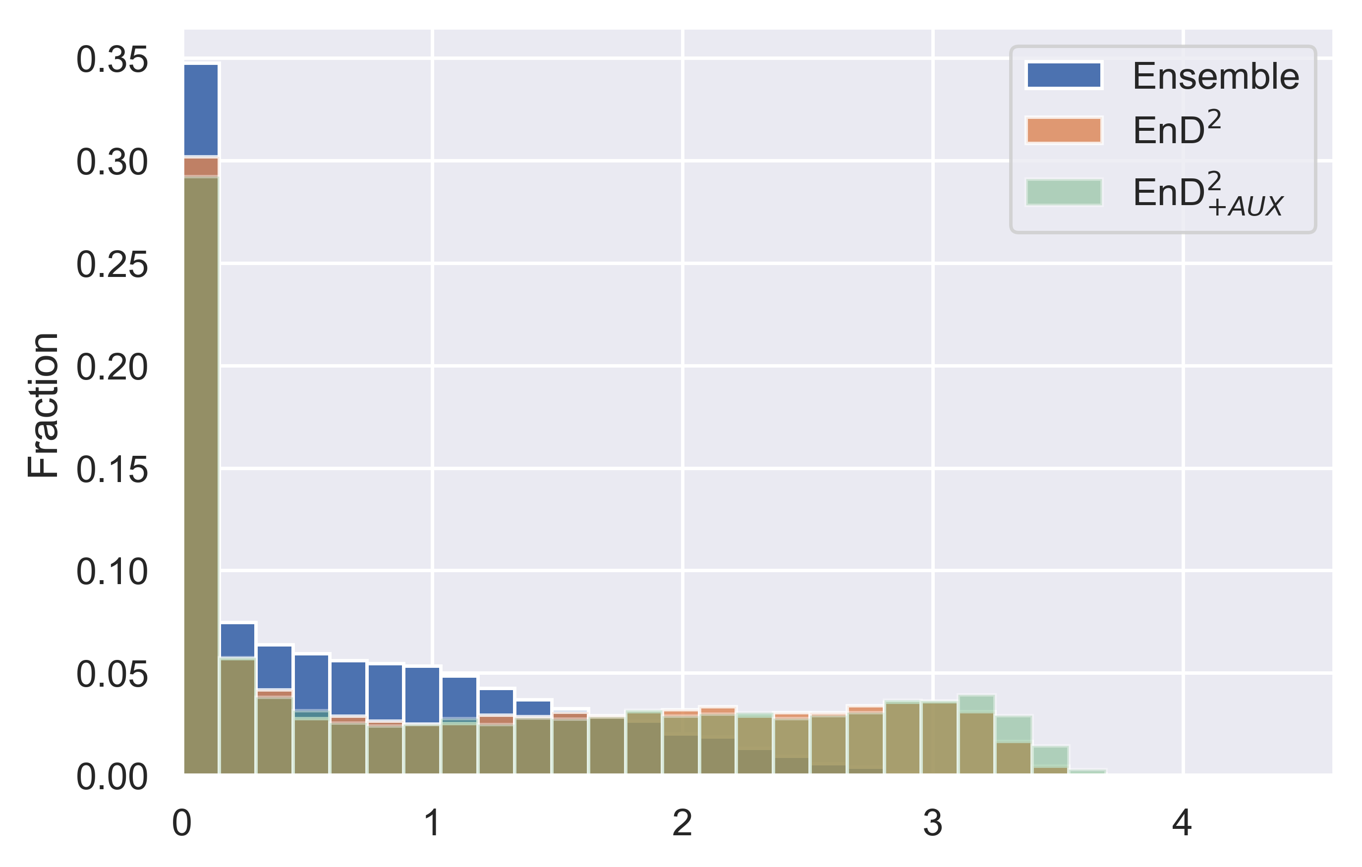
(b) C100 Data Uncert. - ID

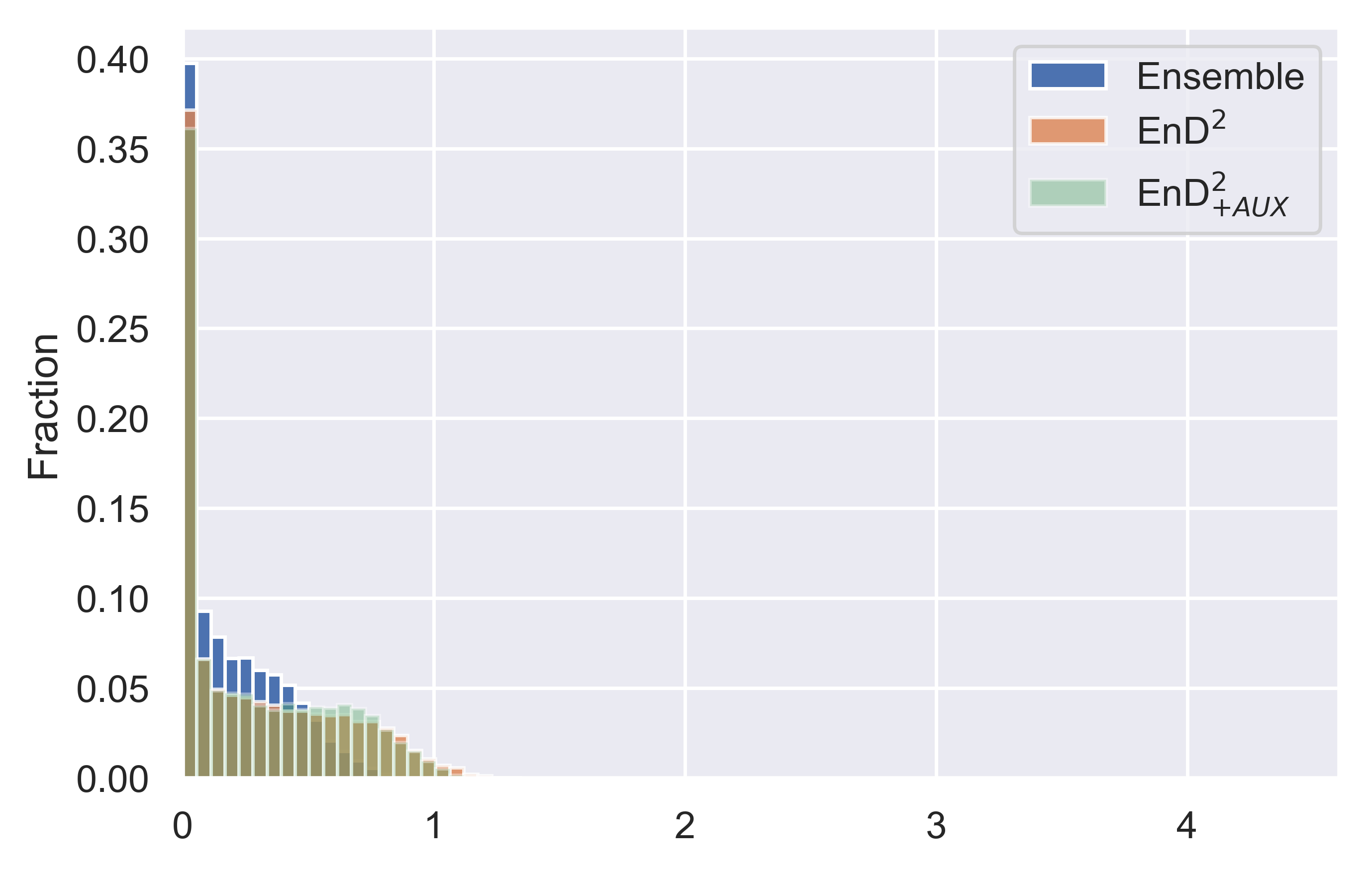
(c) C100 Knowledge Uncert. - OOD

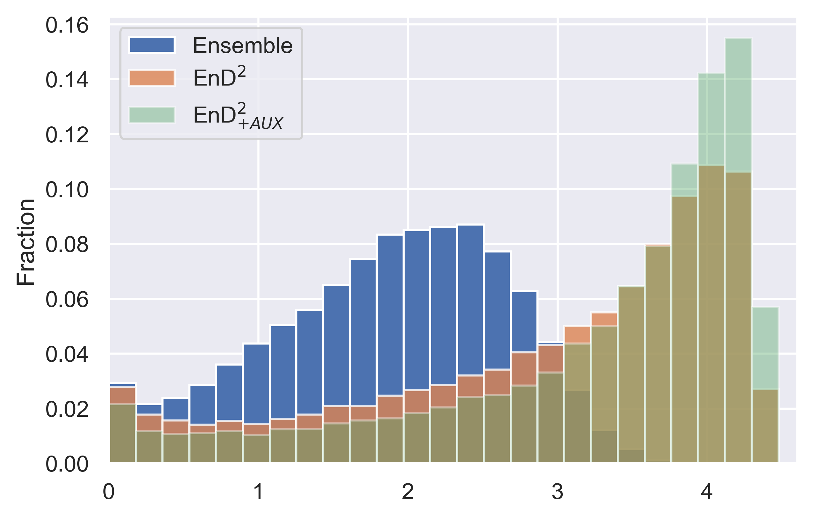
(d) C100 Total Uncert. - OOD

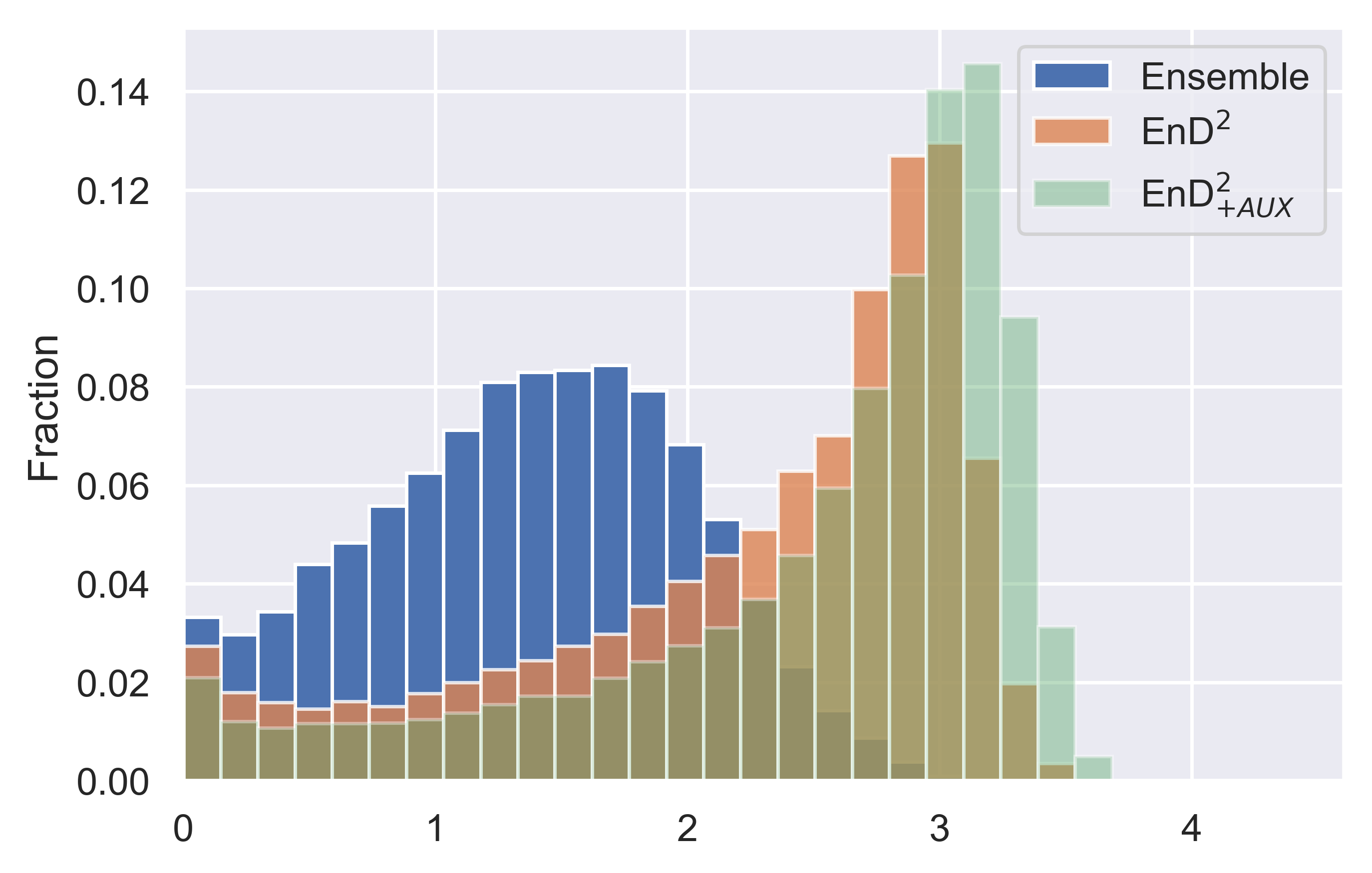
(e) C100 Data Uncert. - OOD

(f) C100 Knowledge Uncert. - OOD

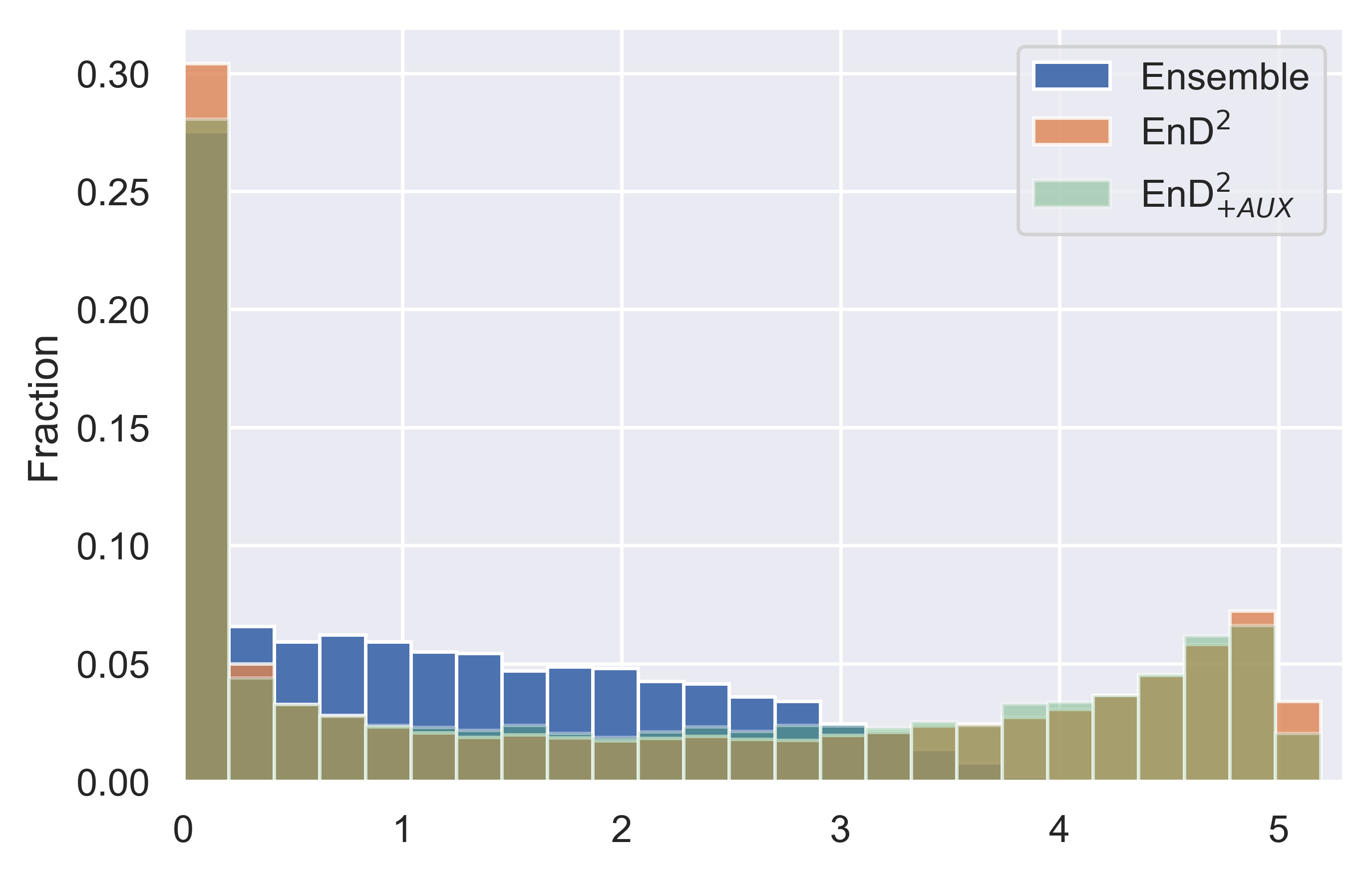
(g) TIM Total Uncert. - ID

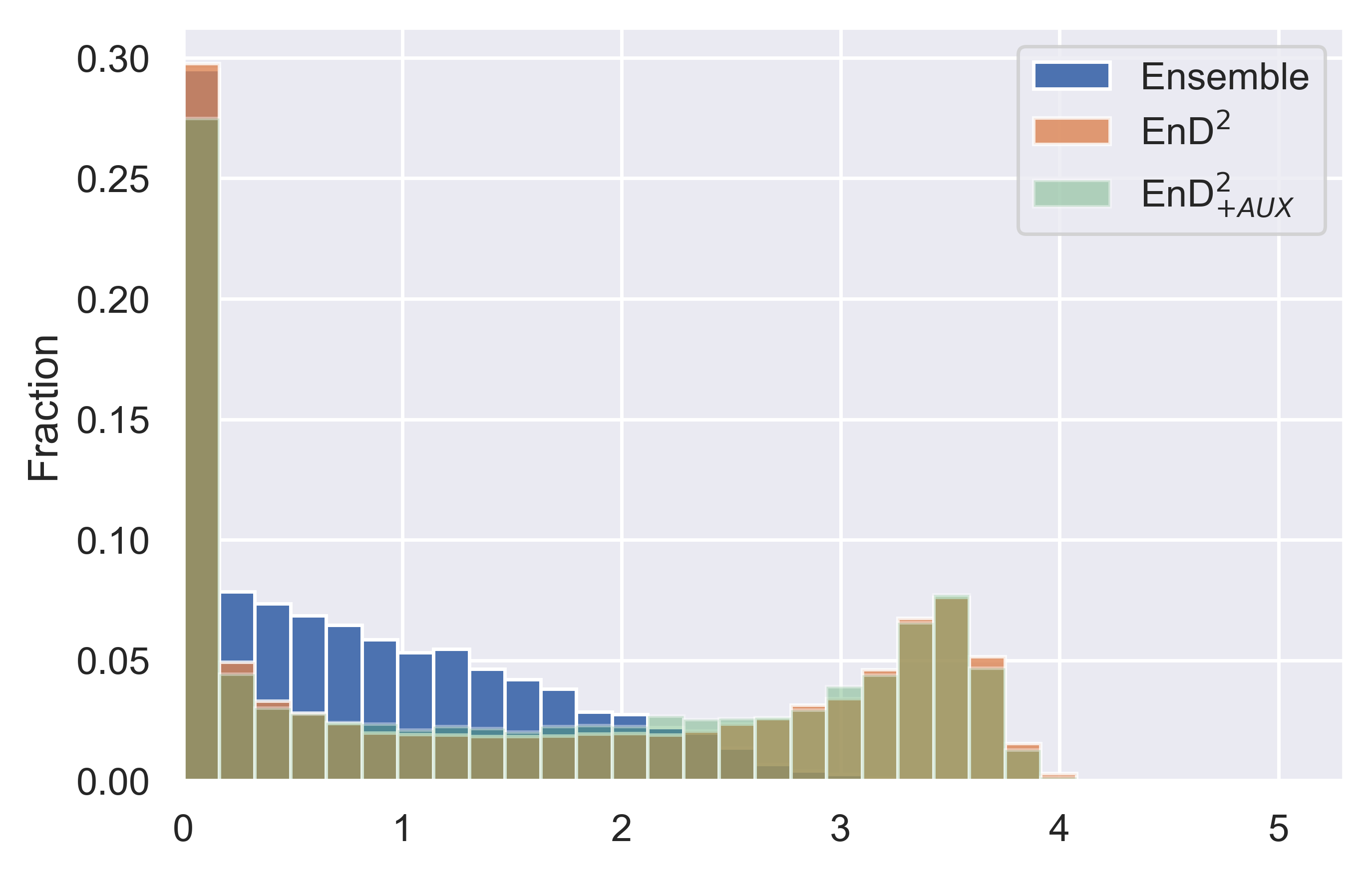
(h) TIM Data Uncert. - ID

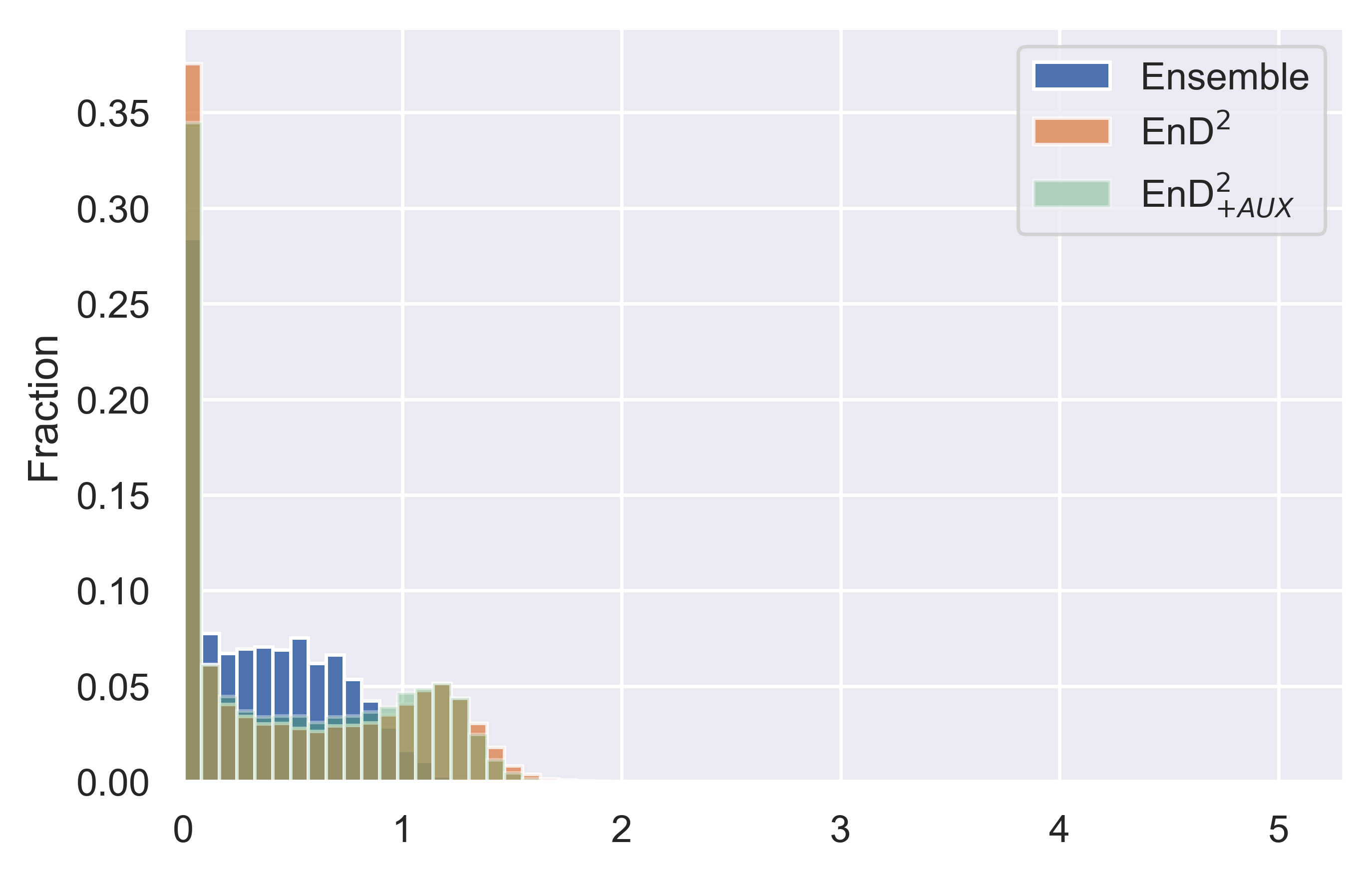
(i) TIM Knowledge Uncert. - OOD

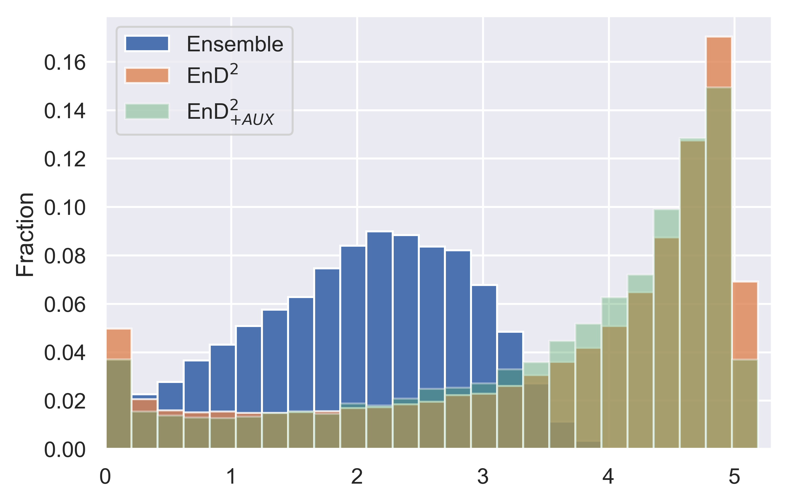
(j) TIM Total Uncert. - OOD

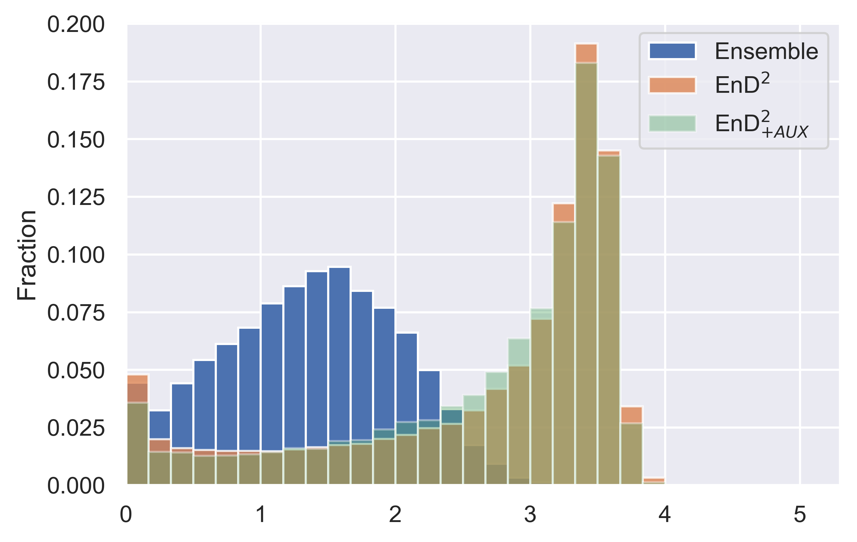
(k) TIM Data Uncert. - OOD

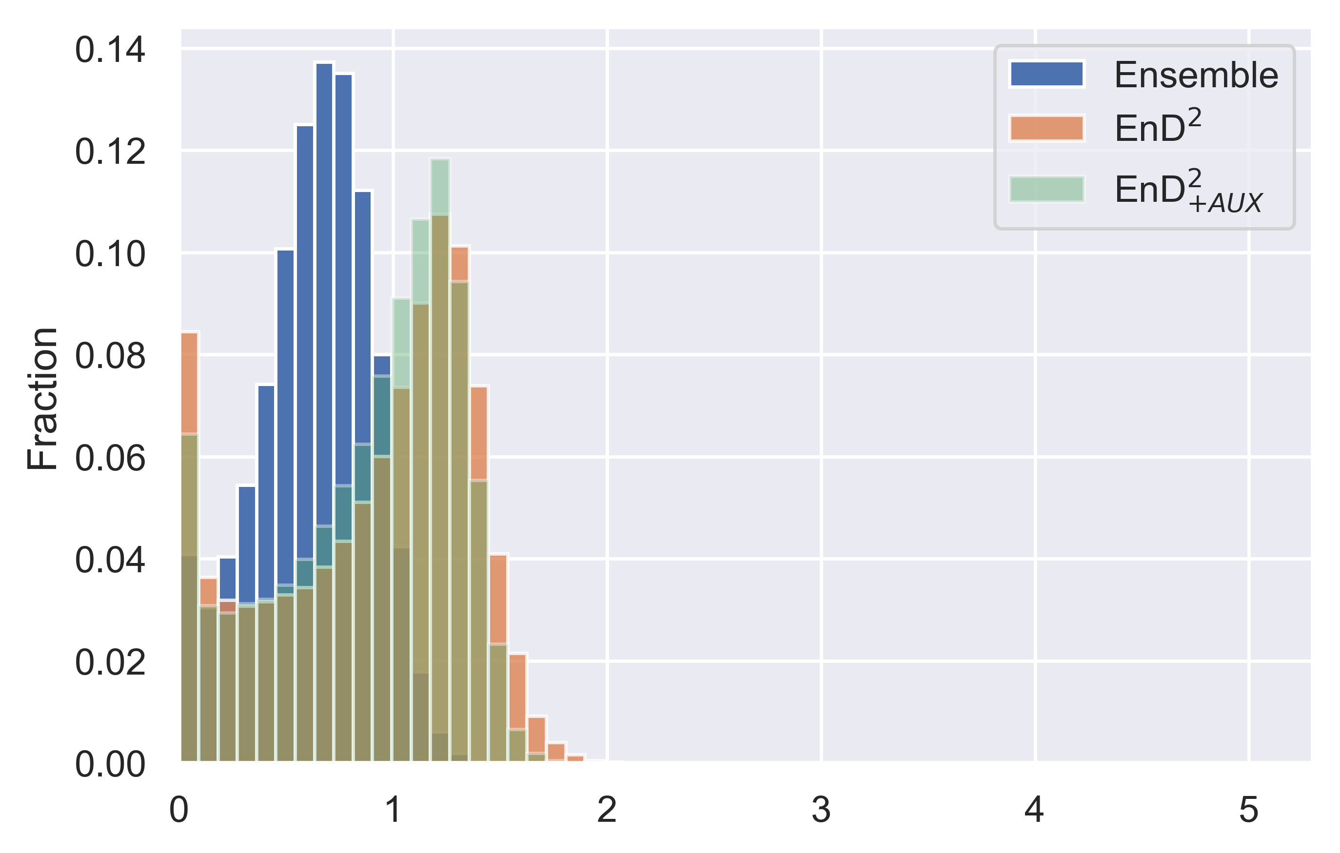
(l) TIM Knowledge Uncert. - OOD

Figure 6: Histograms of measures of uncertainty derived from ensemble, EnD² and EnD${}^{2}_{\tt+AUX}$ on in-domain (ID) and test out-of-domain (OOD) data from CIFAR-100 and TinyImageNet.

In addition, we have also provided histograms of total uncertainty for EnD and EnD_+AUX models trained on CIFAR-10, CIFAR-100 and TinyImageNet relative to the ensemble for both in-domain and OOD data. Figure 7 shows that while all EnD models match the uncertainty of the ensemble on in-domain data for all datasets, EnD consistently under-estimates the uncertainty for OOD data. The only exception is EnD_+AUX on CIFAR-100, where it matches the ensemble’s predictions well. This generally agrees with the results from section 5, where EnD_+AUX is able to almost match the ensemble’s OOD detection performance.

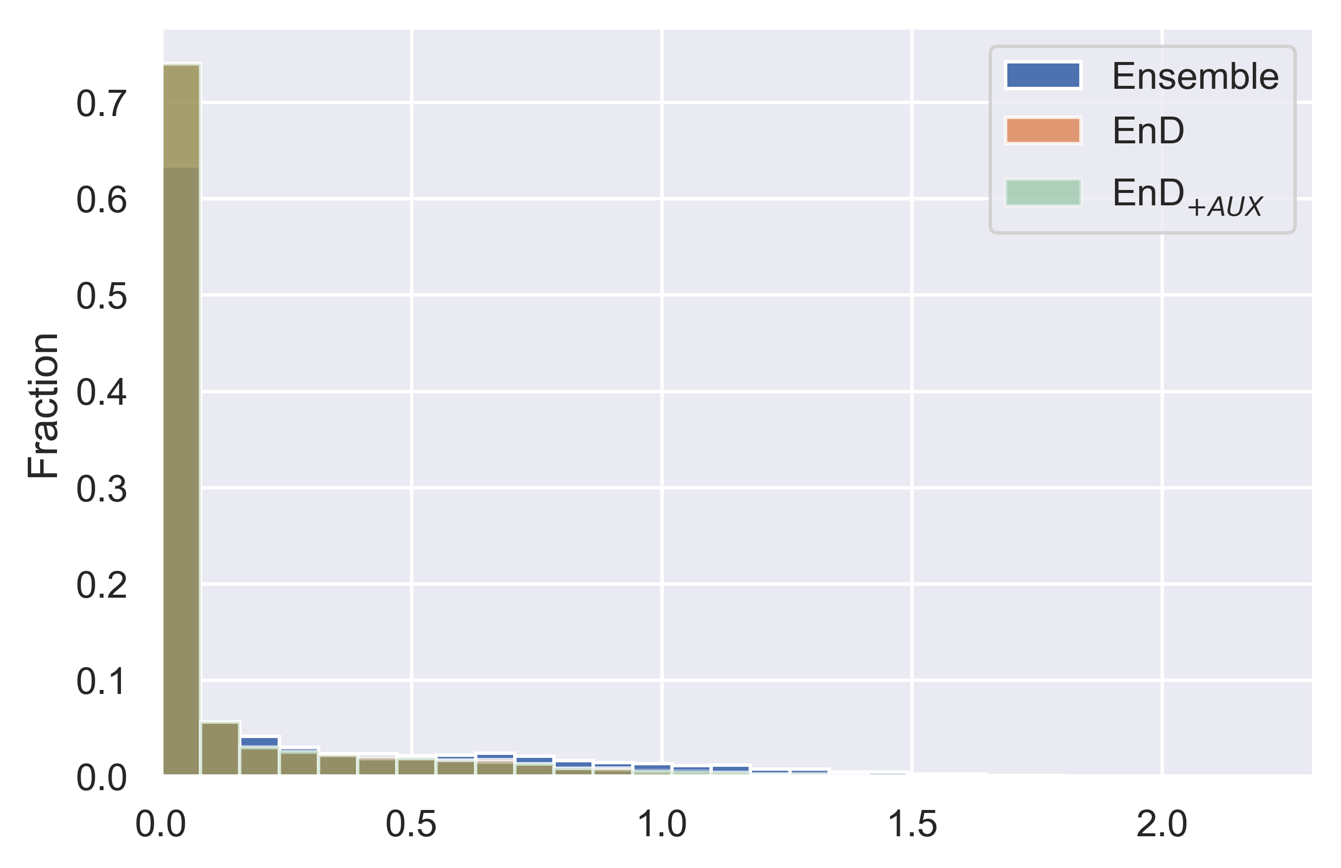
(a) C10 Total Uncertainty - ID

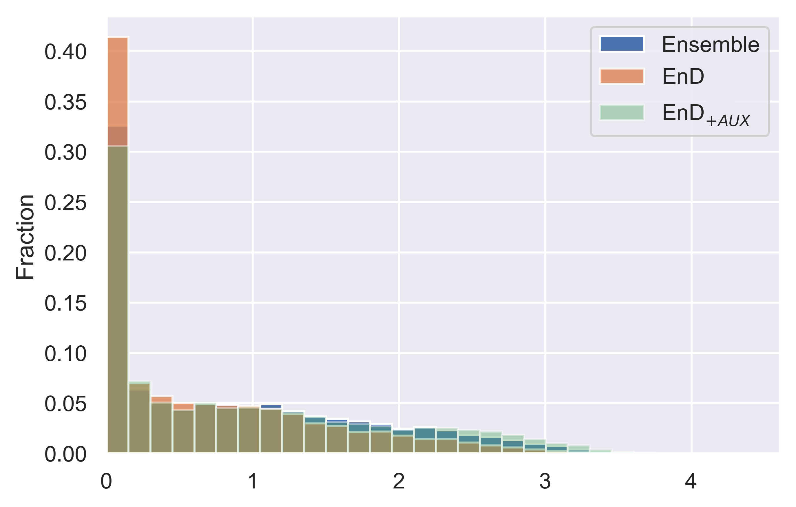
(b) C100 Total Uncertainty - ID

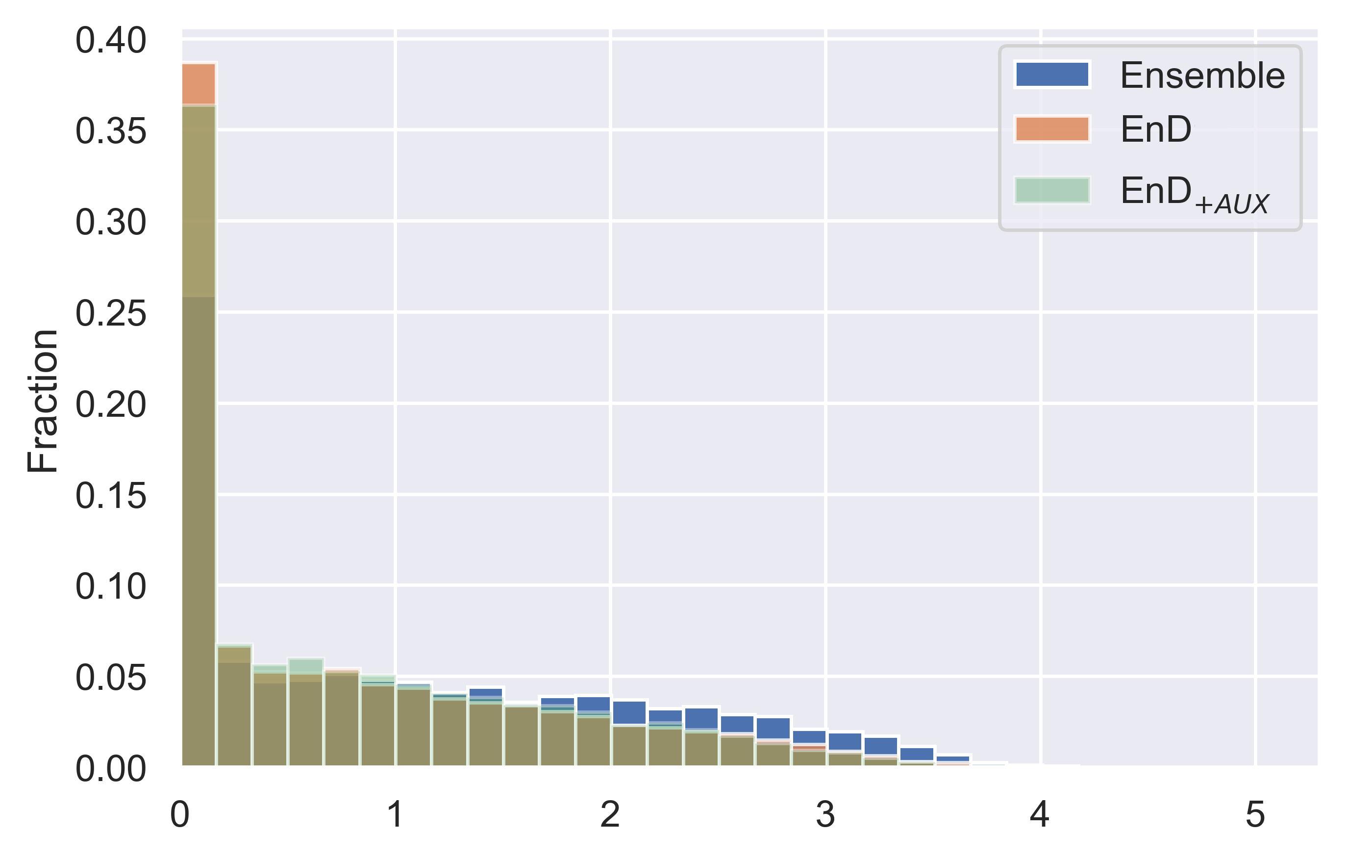
(c) TIM Total Uncertainty - ID

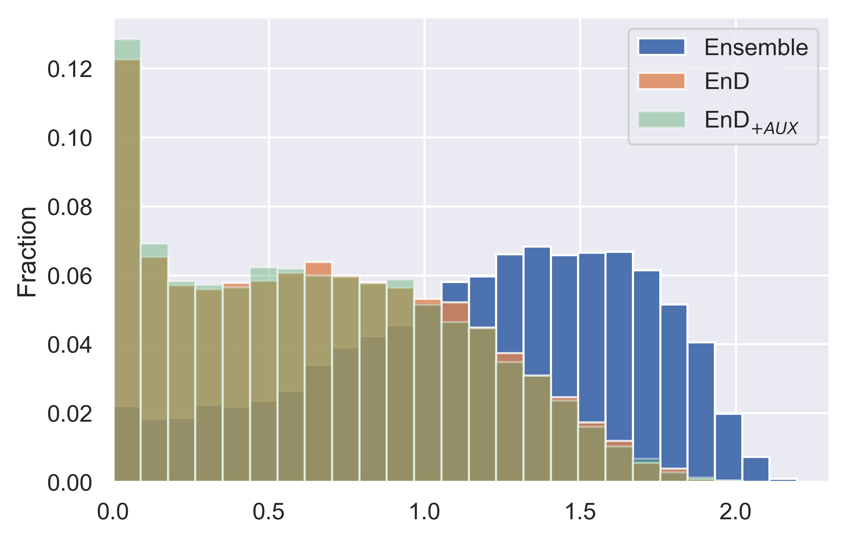
(d) C10 Total Uncertainty - OOD

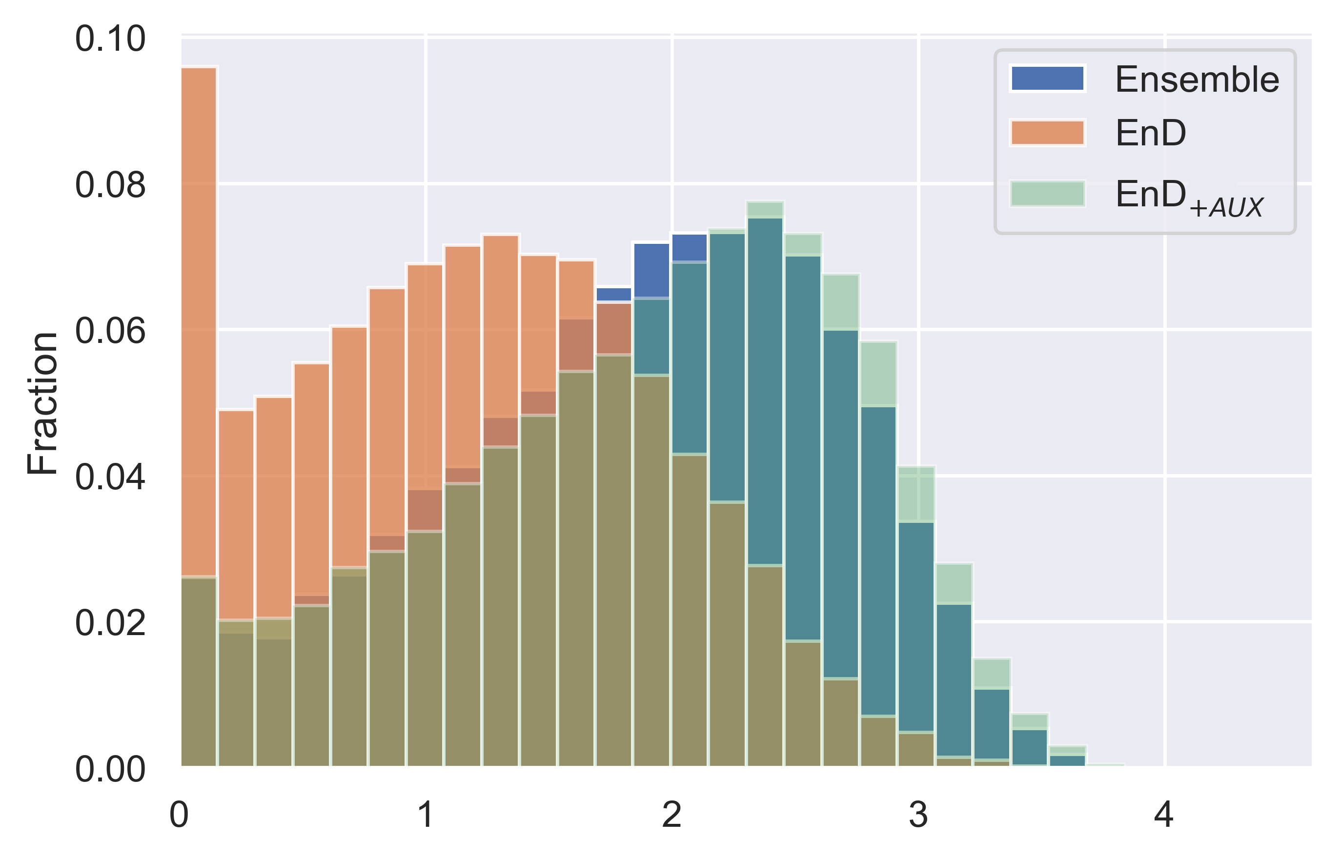
(e) C100 Total Uncertainty - OOD

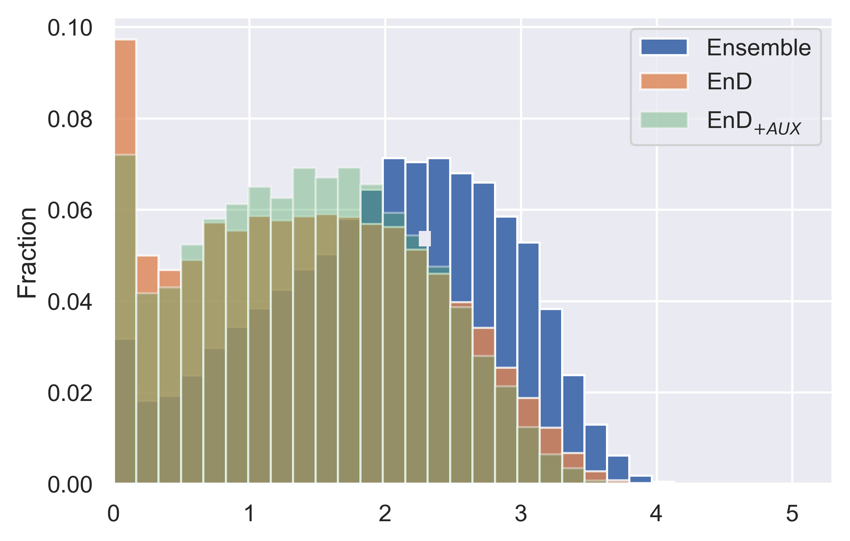
(f) TIM Total Uncertainty - OOD

Figure 7: Histograms of measures of total uncertainty derived from ensemble EnD, and EnD_+AUX on in-domain (ID) and test out-of-domain (OOD) data.

Appendix D Ablation Studies

In this paper we made several important design choices. Firstly, we chose to use rich ensembles of 100 models, in order to generate a good estimate of the empirical distribution of the ensemble on the simplex and assess whether the Dirichlet distribution was flexible enough to model it. Secondly, we used a temperature annealing schedule with an initial temperature of 10. In this section we conduct two ablation studies. Firstly, we assess whether Ensemble Distribution Distillation is possible when using an ensemble of 5, 20, 50 and 100 models. Secondly, we investigate a range of initial temperatures (1, 2, 5, 10, and 20) for temperature annealing for the models trained on the CIFAR-10 and CIFAR-100 datasets. Here, only the EnD${}^{2}_{+AUX}$ model is considered. Results are presented in figures 8-13. All figures depict the mean across 3 models (for each configuration) $\pm$ 1 standard deviation.

Overall, the results show two important trends. Firstly, using using 20 models does better than using 5 models, but there are no conclusive gains for ensemble distribution distillation from using more than 20 models. This suggests that it is sufficient to use ensemble of fewer models for Ensemble Distribution Distillation with models which parameterize the Dirichlet Distribution. This is beneficial in terms computation and memory savings. It is possible, however, that if a more flexible distribution is used, such as a Mixture of Dirichlets, then it might be possible to derive further gains from a larger ensemble. The second trend is that it is necessary to use a temperature of at least 5 in order to successfully distribution-distill the ensemble. Using initial temperatures of 10 and 20 did not result in any significant further increase in performance. These results show that the temperature annealing process is important for Ensemble Distribution Distillation to work well.

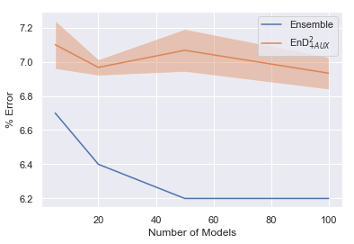
(a) % Classification Error

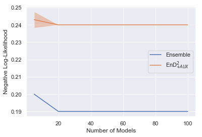
(b) Negative Log-likelihood

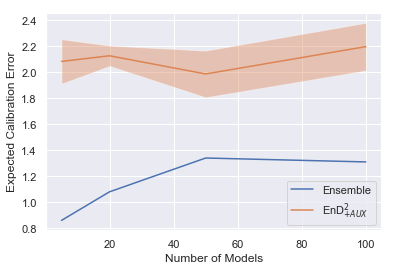
(c) Expected Calibration Error

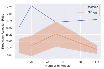
(d) Prediction Rejection Ratio

Figure 8: CIFAR-10 Model Ablation

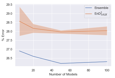
(a) % Classification Error

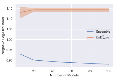
(b) Negative Log-likelihood

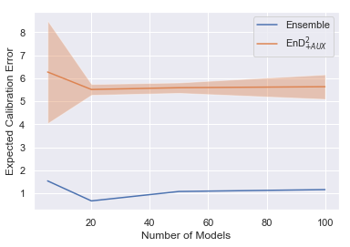
(c) Expected Calibration Error

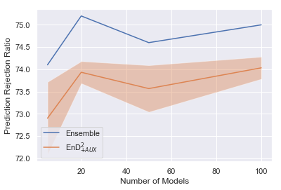
(d) Prediction Rejection Ratio

Figure 9: CIFAR-100 Model Ablation

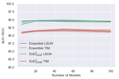
(a) C10 Total Uncertainty

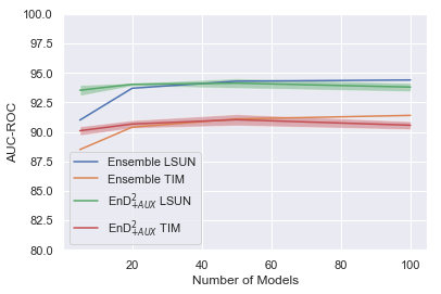
(b) C10 Knowledge Uncertainty

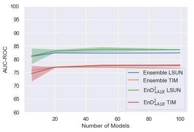
(c) C100 Total Uncertainty

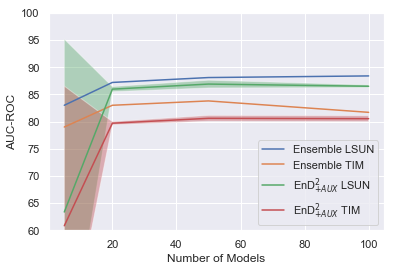
(d) C100 Knowledge Uncertainty

Figure 10: CIFAR-10 and CIFAR-100 Model Ablation - Uncertainties

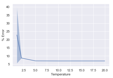
(a) % Classification Error

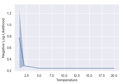
(b) Negative Log-likelihood

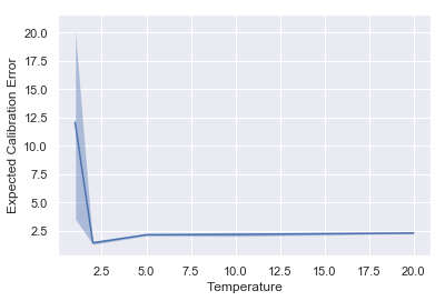
(c) Expected Calibration Error

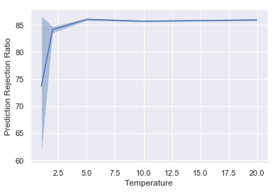
(d) Prediction Rejection Ratio

Figure 11: CIFAR-10 Temperature Ablation

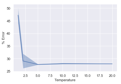
(a) % Classification Error

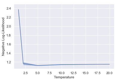
(b) Negative Log-likelihood

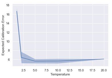
(c) Expected Calibration Error

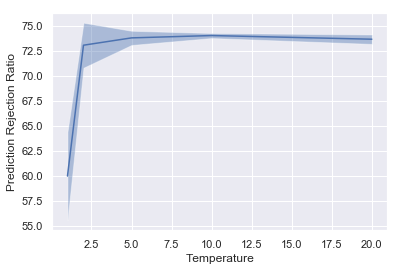
(d) Prediction Rejection Ratio

Figure 12: CIFAR-100 Temperature Ablation

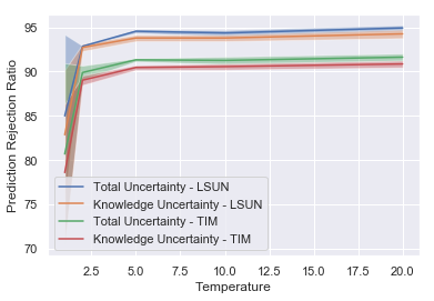
(a) CIFAR-10 Uncertainties

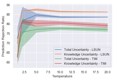
(b) CIFAR-100 Uncertainties

Figure 13: CIFAR-10 and CIFAR-100 Temperature Ablation - Uncertainties

References

- Alipanahi et al. (2015) Babak Alipanahi, Andrew Delong, Matthew T. Weirauch, and Brendan J. Frey. Predicting the sequence specificities of DNA- and RNA-binding proteins by deep learning. Nature Biotechnology, 33(8):831–838, July 2015. ISSN 1087-0156. doi: 10.1038/nbt.3300. URL http://dx.doi.org/10.1038/nbt.3300.
- Amodei et al. (2016) Dario Amodei, Chris Olah, Jacob Steinhardt, Paul F. Christiano, John Schulman, and Dan Mané. Concrete problems in AI safety. http://arxiv.org/abs/1606.06565, 2016. arXiv: 1606.06565.
- Buciluǎ et al. (2006) Cristian Buciluǎ, Rich Caruana, and Alexandru Niculescu-Mizil. Model compression. In Proceedings of the 12th ACM SIGKDD International Conference on Knowledge Discovery and Data Mining, KDD ’06, pp. 535–541, New York, NY, USA, 2006. ACM. ISBN 1-59593-339-5. doi: 10.1145/1150402.1150464. URL http://doi.acm.org/10.1145/1150402.1150464.
- Caruana et al. (2015) Rich Caruana, Yin Lou, Johannes Gehrke, Paul Koch, Marc Sturm, and Noemie Elhadad. Intelligible models for healthcare: Predicting pneumonia risk and hospital 30-day readmission. In Proc. 21th ACM SIGKDD International Conference on Knowledge Discovery and Data Mining, KDD ’15, pp. 1721–1730, New York, NY, USA, 2015. ACM. ISBN 978-1-4503-3664-2. doi: 10.1145/2783258.2788613. URL http://doi.acm.org/10.1145/2783258.2788613.
- CS231N (2017) Stanford CS231N. Tiny ImageNet. https://tiny-imagenet.herokuapp.com/, 2017.
- De Fauw et al. (2018) Jeffrey De Fauw, Joseph R Ledsam, Bernardino Romera-Paredes, Stanislav Nikolov, Nenad Tomasev, Sam Blackwell, Harry Askham, Xavier Glorot, Brendan O’Donoghue, Daniel Visentin, et al. Clinically applicable deep learning for diagnosis and referral in retinal disease. Nature medicine, 24(9):1342, 2018.
- Depeweg et al. (2017a) Stefan Depeweg, José Miguel Hernández-Lobato, Finale Doshi-Velez, and Steffen Udluft. Decomposition of uncertainty for active learning and reliable reinforcement learning in stochastic systems. stat, 1050:11, 2017a.
- Depeweg et al. (2017b) Stefan Depeweg, José Miguel Hernández-Lobato, Finale Doshi-Velez, and Steffen Udluft. Decomposition of uncertainty in bayesian deep learning for efficient and risk-sensitive learning. arXiv preprint arXiv:1710.07283, 2017b.
- Englesson & Azizpour (2019) Erik Englesson and Hossein Azizpour. Efficient evaluation-time uncertainty estimation by improved distillation. arXiv preprint arXiv:1906.05419, 2019.
- Gal (2016) Yarin Gal. Uncertainty in Deep Learning. PhD thesis, University of Cambridge, 2016.
- Gal & Ghahramani (2016) Yarin Gal and Zoubin Ghahramani. Dropout as a Bayesian Approximation: Representing Model Uncertainty in Deep Learning. In Proc. 33rd International Conference on Machine Learning (ICML-16), 2016.
- Garipov et al. (2018) Timur Garipov, Pavel Izmailov, Dmitrii Podoprikhin, Dmitry P Vetrov, and Andrew G Wilson. Loss surfaces, mode connectivity, and fast ensembling of dnns. In S. Bengio, H. Wallach, H. Larochelle, K. Grauman, N. Cesa-Bianchi, and R. Garnett (eds.), Advances in Neural Information Processing Systems 31, pp. 8803–8812. Curran Associates, Inc., 2018. URL http://papers.nips.cc/paper/8095-loss-surfaces-mode-connectivity-and-fast-ensembling-of-dnns.pdf.
- Girshick (2015) Ross Girshick. Fast R-CNN. In Proc. 2015 IEEE International Conference on Computer Vision (ICCV), pp. 1440–1448, 2015.
- Hannun et al. (2014) Awni Y. Hannun, Carl Case, Jared Casper, Bryan Catanzaro, Greg Diamos, Erich Elsen, Ryan Prenger, Sanjeev Satheesh, Shubho Sengupta, Adam Coates, and Andrew Y. Ng. Deep speech: Scaling up end-to-end speech recognition, 2014. URL http://arxiv.org/abs/1412.5567. arXiv:1412.5567.
- He et al. (2016) Kaiming He, Xiangyu Zhang, Shaoqing Ren, and Jian Sun. Deep residual learning for image recognition. In Proc. 2016 IEEE Conference on Computer Vision and Pattern Recognition (CVPR), pp. 770–778, 2016.
- Hendrycks & Gimpel (2016) Dan Hendrycks and Kevin Gimpel. A Baseline for Detecting Misclassified and Out-of-Distribution Examples in Neural Networks. http://arxiv.org/abs/1610.02136, 2016. arXiv:1610.02136.
- Hinton et al. (2012) Geoffrey Hinton, Li Deng, Dong Yu, George Dahl, Abdel rahman Mohamed, Navdeep Jaitly, Andrew Senior, Vincent Vanhoucke, Patrick Nguyen, Tara Sainath, and Brian Kingsbury. Deep neural networks for acoustic modeling in speech recognition. Signal Processing Magazine, 2012.
- Hinton et al. (2015) Geoffrey Hinton, Oriol Vinyals, and Jeffrey Dean. Distilling the knowledge in a neural network. In NIPS Deep Learning and Representation Learning Workshop, 2015. URL http://arxiv.org/abs/1503.02531.
- Kingma & Ba (2015) Diederik P. Kingma and Jimmy Ba. Adam: A Method for Stochastic Optimization. In Proc. 3rd International Conference on Learning Representations (ICLR), 2015.
- Korattikara Balan et al. (2015) Anoop Korattikara Balan, Vivek Rathod, Kevin P Murphy, and Max Welling. Bayesian dark knowledge. In C. Cortes, N. D. Lawrence, D. D. Lee, M. Sugiyama, and R. Garnett (eds.), Advances in Neural Information Processing Systems 28, pp. 3438–3446. Curran Associates, Inc., 2015. URL http://papers.nips.cc/paper/5965-bayesian-dark-knowledge.pdf.
- Krizhevsky (2009) Alex Krizhevsky. Learning multiple layers of features from tiny images. 2009. URL https://www.cs.toronto.edu/~kriz/learning-features-2009-TR.pdf.
- Lakshminarayanan et al. (2017) B. Lakshminarayanan, A. Pritzel, and C. Blundell. Simple and Scalable Predictive Uncertainty Estimation using Deep Ensembles. In Proc. Conference on Neural Information Processing Systems (NIPS), 2017.
- LeCun et al. (2015) Yann LeCun, Yoshua Bengio, and Geoffrey Hinton. Deep learning. nature, 521(7553):436, 2015.
- Li & Hoiem (2019) Zhizhong Li and Derek Hoiem. Reducing overconfident errors outside the known distribution, 2019. URL https://openreview.net/forum?id=S1giro05t7.
- Maddox et al. (2019) Wesley Maddox, Timur Garipov, Pavel Izmailov, Dmitry Vetrov, and Andrew Gordon Wilson. A simple baseline for bayesian uncertainty in deep learning. arXiv preprint arXiv:1902.02476, 2019.
- Malinin et al. (2017) A. Malinin, A. Ragni, M.J.F. Gales, and K.M. Knill. Incorporating Uncertainty into Deep Learning for Spoken Language Assessment. In Proc. 55th Annual Meeting of the Association for Computational Linguistics (ACL), 2017.
- Malinin (2019) Andrey Malinin. Uncertainty Estimation in Deep Learning with application to Spoken Language Assessment. PhD thesis, University of Cambridge, 2019.
- Malinin & Gales (2018) Andrey Malinin and Mark Gales. Predictive uncertainty estimation via prior networks. In Advances in Neural Information Processing Systems, pp. 7047–7058, 2018.
- Malinin & Gales (2019) Andrey Malinin and Mark Gales. Reverse kl-divergence training of prior networks: Improved uncertainty and adversarial robustness. Advances in Neural Information Processing Systems, 2019.
- Mikolov et al. (2010) Tomas Mikolov, Martin Karafiát, Lukás Burget, Jan Cernocký, and Sanjeev Khudanpur. Recurrent Neural Network Based Language Model. In Proc. INTERSPEECH, 2010.
- Mikolov et al. (2013a) Tomas Mikolov, Kai Chen, Greg Corrado, and Jeffrey Dean. Efficient Estimation of Word Representations in Vector Space, 2013a. URL http://arxiv.org/abs/1301.3781. arXiv:1301.3781.
- Mikolov et al. (2013b) Tomas Mikolov et al. Linguistic Regularities in Continuous Space Word Representations. In Proc. NAACL-HLT, 2013b.
- Murphy (2012) Kevin P. Murphy. Machine Learning. The MIT Press, 2012.
- Osband et al. (2016) Ian Osband, Charles Blundell, Alexander Pritzel, and Benjamin Van Roy. Deep exploration via bootstrapped dqn. In D. D. Lee, M. Sugiyama, U. V. Luxburg, I. Guyon, and R. Garnett (eds.), Advances in Neural Information Processing Systems 29, pp. 4026–4034. Curran Associates, Inc., 2016. URL http://papers.nips.cc/paper/6501-deep-exploration-via-bootstrapped-dqn.pdf.
- Ovadia et al. (2019) Yaniv Ovadia, Emily Fertig, Jie Ren, Zachary Nado, D Sculley, Sebastian Nowozin, Joshua V Dillon, Balaji Lakshminarayanan, and Jasper Snoek. Can you trust your model’s uncertainty? evaluating predictive uncertainty under dataset shift. arXiv preprint arXiv:1906.02530, 2019.
- Papamakarios (2015) George Papamakarios. Distilling model knowledge. arXiv preprint arXiv:1510.02437, 2015.
- Paszke et al. (2017) Adam Paszke, Sam Gross, Soumith Chintala, Gregory Chanan, Edward Yang, Zachary DeVito, Zeming Lin, Alban Desmaison, Luca Antiga, and Adam Lerer. Automatic differentiation in PyTorch. In NIPS Autodiff Workshop, 2017.
- Quiñonero-Candela (2009) Joaquin Quiñonero-Candela. Dataset Shift in Machine Learning. The MIT Press, 2009.
- Schroff et al. (2015) Florian Schroff, Dmitry Kalenichenko, and James Philbin. Facenet: A unified embedding for face recognition and clustering. In Proceedings of the IEEE conference on computer vision and pattern recognition, pp. 815–823, 2015.
- Simonyan & Zisserman (2015) Karen Simonyan and Andrew Zisserman. Very Deep Convolutional Networks for Large-Scale Image Recognition. In Proc. International Conference on Learning Representations (ICLR), 2015.
- Smith & Gal (2018) L. Smith and Y. Gal. Understanding Measures of Uncertainty for Adversarial Example Detection. In UAI, 2018.
- Villegas et al. (2017) Ruben Villegas, Jimei Yang, Yuliang Zou, Sungryull Sohn, Xunyu Lin, and Honglak Lee. Learning to Generate Long-term Future via Hierarchical Prediction. In Proc. International Conference on Machine Learning (ICML), 2017.
- Wang et al. (2018) Y. Wang, J. H. M. Wong, M. J. F. Gales, K. M. Knill, and A. Ragni. Sequence teacher-student training of acoustic models for automatic free speaking language assessment. In 2018 IEEE Spoken Language Technology Workshop (SLT), pp. 994–1000, 2018. doi: 10.1109/SLT.2018.8639557.
- Welling & Teh (2011) Max Welling and Yee Whye Teh. Bayesian Learning via Stochastic Gradient Langevin Dynamics. In Proc. International Conference on Machine Learning (ICML), 2011.
- Wong & Gales (2017) J. H. M. Wong and M. J. F. Gales. Multi-task ensembles with teacher-student training. In 2017 IEEE Automatic Speech Recognition and Understanding Workshop (ASRU), pp. 84–90, 2017. doi: 10.1109/ASRU.2017.8268920.
- Yu et al. (2015) Fisher Yu, Yinda Zhang, Shuran Song, Ari Seff, and Jianxiong Xiao. LSUN: construction of a large-scale image dataset using deep learning with humans in the loop, 2015. URL http://arxiv.org/abs/1506.03365. arXiv:1506.03365.