Categorical Feature Compression via Submodular Optimization

Abstract

In the era of big data, learning from categorical features with very large vocabularies (e.g., 28 million for the Criteo click prediction dataset) has become a practical challenge for machine learning researchers and practitioners. We design a highly-scalable vocabulary compression algorithm that seeks to maximize the mutual information between the compressed categorical feature and the target binary labels and we furthermore show that its solution is guaranteed to be within a $1-1/e\approx 63\%$ factor of the global optimal solution. To achieve this, we introduce a novel re-parametrization of the mutual information objective, which we prove is submodular, and design a data structure to query the submodular function in amortized $O(\log n)$ time (where $n$ is the input vocabulary size). Our complete algorithm is shown to operate in $O(n\log n)$ time. Additionally, we design a distributed implementation in which the query data structure is decomposed across $O(k)$ machines such that each machine only requires $O(\frac{n}{k})$ space, while still preserving the approximation guarantee and using only logarithmic rounds of computation. We also provide analysis of simple alternative heuristic compression methods to demonstrate they cannot achieve any approximation guarantee. Using the large-scale Criteo learning task, we demonstrate better performance in retaining mutual information and also verify competitive learning performance compared to other baseline methods.

1 Introduction

In modern large scale machine learning tasks, the presence of categorical features with extremely large vocabularies is a standard occurrence. For example, in tasks such as product recommendation and click-through rate prediction, categorical variables corresponding to inventory id, webpage identifier, or other such high cardinality values, can easily contain anywhere from hundreds of thousands to tens of millions of unique values. The size of machine learning models generally grows at least linearly with the vocabulary size and, thus, the memory required to serve the model, the training and inference cost, as well as the risk of overfitting become an issue with very large vocabularies. In the particular case of neural networks model, one generally uses an embedding layer to consume categorical inputs. The number of parameters in the embedding layer is $O(nh)$, where $n$ is the size of the vocabulary and $h$ is the number of units in the first hidden layer.

To give a concrete example, the Criteo click prediction benchmark has about 28 million categorical feature values (CriteoLabs, 2014), thus resulting in an embedding layer more than 1 billion parameters for a modestly sized first hidden layer. Note, this number dwarfs the number of parameters found in the remainder of the neural network. Again, to give a concrete example, even assuming a very deep fully connected network of depth $10^{2}$ with hidden layers of size $10^{3}$, we have $(10^{3}\times 10^{3})10^{2}=10^{8}$ parameters in the hidden network – still an order of magnitude smaller than the embedding layer alone. This motivates the problem of compressing the vocabulary into a smaller size while still retaining as much information as possible.

In this work, we model the compression task by considering the problem of maximizing the mutual information between the compressed version of the categorical features and the target label. We first observe a connection between this problem and the quantization problem for discrete memoryless channels, and note a polynomial-time algorithm for the problem (Kurkoski and Yagi, 2014; Iwata and Ozawa, 2014). The resulting algorithm, however, is based on solving a quadratic-time dynamic program, and is not scalable. Our main goal in this paper is to develop a scalable and distributed algorithm with a guaranteed approximation factor. We achieve this goal by developing a novel connection to submodular optimization. Although in some settings, entropy-based set functions are known to be submodular, this is not the case for the mutual information objective we consider (mutual information with respect to the target labels). Our main insight is in proving the submodularity of a particular transformation of the mutual information objective, which still allows us to provide an approximation guarantee on the quality of the solution with respect to the original objective. We also provide a data structure that allows us to query this newly defined submodular function in amortized logarithmic time. This logarithmic-time implementation of the submodular oracle empowers us to incorporate the fastest known algorithm for submodular maximization (Mirzasoleiman et al., 2015), which leads us to a sequential quasi-linear-time $(1-1/e-\epsilon)$-approximation algorithm for binary vocabulary compression. Next, we provide a distributed implementation for binary vocabulary compression. Previous distributed algorithms for submodular maximization assume a direct access the query oracle on every machine (e.g., see (Barbosa et al., 2015; Mirrokni and Zadimoghaddam, 2015; Mirzasoleiman et al., 2013)). However, the query oracle itself requires $O(n)$ space, which may be restrictive in the large scale setting. In this work, we provide a truly distributed implementation of the submodular maximization algorithm of (Badanidiyuru and Vondrák, 2014) (or similarly  (Kumar et al., 2015)) for our application by distributing the query oracle. In this distributed implementation we manage to decompose the query oracle across $O(k)$ machines such that each machine only requires $O(\frac{n}{k})$ space to store the partial query oracle. As a result, we successfully provide a distributed $(1-1/e-\epsilon)$-approximation algorithm for vocabulary compression in logarithmic rounds of computation. Our structural results for submodularity of this new set function is the main technical contribution of this paper, and can also be of independent interest in other settings that seek to maximize mutual information.

We also study a number of heuristic and baseline algorithms for the problem of maximizing mutual information, and show that they do not achieve a guaranteed approximation for the problem. Furthermore, we study the empirical performance of our algorithms on two fronts: First, we show the effectiveness of our greedy scalable approximation algorithm for maximizing mutual information. Our study confirms that this algorithm not only achieves a theoretical guarantee, but also it beats the heuristic algorithms for maximizing mutual information. Finally, we examine the performance of this algorithm on the vocabulary compression problem itself, and confirm the effectiveness of the algorithm in producing a high-quality solution for vocabulary compression large scale learning tasks.

Organization. In the remainder of this section we review related previous works and introduce the problem formally along with appropriate notation. Then in Section 2, we introduce the novel compression algorithm and corresponding theoretical guarantees as well as analysis of some basic heuristic baselines. In Section 3, we present our empirical evaluation of optimizing the mutual information objective as well as an end-to-end learning task.

1.1 Related Work

Feature Clustering: The use of vocabulary compression has been studied previously, especially in text classification applications where it is commonly known as feature (or word) clustering. In particular, Baker and McCallum (1998) and Slonim and Tishby (2001) both propose agglomerative clustering algorithms, which start with singleton clusters that are iteratively merged using a Jenson-Shannon divergence based function to measure similarity between clusters, until the desired number of clusters is found. Both algorithms are greedy in nature and do not provide any guarantee with respect to a global objective. In (Dhillon et al., 2003), the authors introduce an algorithm that empirically performs better than the aforementioned methods and that also seeks to optimize the same global mutual information objective that is analyzed in this work. Their proposed iterative algorithm is guaranteed to improve the objective at each iteration and arrive at a local minimum, however, no guarantee with respect to the global optimum is provided. Furthermore, each iteration of the algorithm requires $O(mn)$ time (where $m$ is the size of the compressed vocabulary) and the number of iterations is only guaranteed to be finite (but potentially exponential). Later in this work, we compare the empirical performance of this algorithm with our proposed method.

Figure 1: Translation of terminologies of the DMC quantizer design problem and the feature compression problem.

Compression in Discrete Memoryless Channels: An area from information theory that is closely related to our vocabulary compression problem, and which our algorithm draws inspiration from, is compression in a discrete memoryless channels (DMC) (Cicalese et al., 2018; Zhang and Kurkoski, 2016; Iwata and Ozawa, 2014). In this problem, we assume there is a DMC which (in machine learning terminology) receive a class label and produces a corresponding categorical feature value drawn according to a fixed underlying distribution. The goal is to design a quantizer that maps the space of categorical features in lower cardinatility set, while preserving as much of the mutual information between the class label and newly constructed vocabulary. In Figure 1, we present a diagram that illustrates the DMC quantization problem and vocabulary compression problem as well as the translation of terminologies of these two problems. The results of Kurkoski and Yagi (2014) are of particular interest, as they show a cubic-time dynamic programming based algorithm is able to provide an optimal solution in the case of binary labels. Following this work, Iwata and Ozawa (2014) improve the computational complexity of this approach to quadratic time using the SMAWK algorithm (Aggarwal et al., 1987). Such algorithms are useful in the smaller scale regime, however, the use of a cubic- or even quadratic-time algorithm will be infeasible for our massive vocabulary size use cases. Finally, Mumey and Gedeon (2003) shows that in the general case of greater than two class labels, finding the optimal compression is NP-complete. In this work, we will be focusing on the binary label setting.

Feature Selection: A related method for dealing with very large vocabularies is to do feature selection, in which we simply select a subset of the vocabulary values and remove the rest (see (Guyon and Elisseeff, 2003) and the many references therein). One can view this approach as a special case of vocabulary compression, where we are restricted to only singleton “clusters”. Restricting the problem by selecting a subset of the vocabulary may have some benefits, such as potentially simplifing the optimization problem and the use of a simple filter to transform data at inference time. However, the obvious downside to this restriction is the loss of information and potentially poorer learning performance (see introduction of (Jiang et al., 2011)). In this work we focus on the more general vocabulary compression setting.

Other Feature Extraction Approaches: Clustering features in order to compress a vocabulary is only one approach to lower dimensional feature extraction. There are of course many classical approaches to feature extraction (see Chapter 15 of (Mohri et al., 2018)), such as learning linear projections (e.g., Principle Component Analysis, Linear Discriminant Analysis) or non-linear transformations (e.g., Locally Linear Embeddings, ISOMAP, Laplacian Eigenmaps). However, these classical methods generally incur more than quasilinear computational cost, for both learning and the application the transformation, and are not feasible for our setting.

1.2 Notation

In the vocabulary compression problem we are given a correlated pair of random variables $X$ (a categorical feature) and $C$ (a label), where $X\in\{1,2,\dots,n\}$ and $C\in\{0,1\}$. We aim to define a random variable $Z\in\{1,2,\dots,m\}$ as a function of $X$ that maximizes the mutual information with the label $C$, i.e., $I(Z;C)$, where for general random variables $A$ and $B$ taking values in $\mathcal{A}$ and $\mathcal{B}$, respectively,

$$I(A;B)=\sum_{A\in\mathcal{A}}\sum_{B\in\mathcal{B}}\Pr\left[A,B\right]\log\Big{(}\frac{\Pr\left[A,B\right]}{\Pr\left[A\right]\Pr\left[B\right]}\Big{)}\,.$$ (1)

Note that $Z$ is a function of $X$ and hence we have $I(Z;C)\leq I(X;C)$. If we let $m\geq n$, $Z=X$ maximizes the mutual information $I(Z;C)$. We are interested in the nontrivial case of $m\ll n$. Intuitively, we are compressing the vocabulary of feature $X$ from size $n$ to a smaller size $m$, while preserving the maximum amount of information about $C$.

2 Algorithm and Analysis

In this section, we first show how to transform the original objective into a set function and then prove that this set function is in fact submodular. Next, we describe the components of a quasi-linear and parallelizable algorithm to optimize the objective. Finally, we consider a few simple intuitive baselines and show that they may create features that fail to capture any mutual information with the label.

2.1 Objective Transformation

Without loss of generality assume $\Pr\left[C=0|X=i\right]$ for $i\in\{1,\ldots,n\}$ is sorted in increasing order. Once the feature values are sorted in this order, Lemma 3 of Kurkoski and Yagi (2014) crucially shows that in the optimum solution each value of $Z$ corresponds to a consecutive subsequence of $\{1,\ldots,n\}$ — this is a significant insight that we take from the quantization for DMC literature. Thus, we will cluster consecutive feature values into $m$ clusters, with each cluster corresponding to a value in the compressed vocabulary of $Z$. Formally, define a function $F(S):2^{\{1,\dots,n-1\}}\rightarrow\mathbb{R}$ as follows: Let $S=\{s_{1},\dots,s_{m-1}\}$, and assume $s_{1}<s_{2}<\dots<s_{m-1}$. For simplicity, and without any loss in quality, we set $s_{0}=0$ and $s_{m}=n$. Let $Z$ be a random variable constructed from $X$ that has value $i$, if and only if $s_{i-1}<X\leq s_{i}$. We define $F(S)=I(Z;C)$. Notice that we have

$$\max_{S\subseteq\{2\dots n-1\}\colon|S|=m-1}F(S)=\max_{Z}I(Z;C)\,,$$

where $Z$ is a function of $X$ with vocabulary size $m$. The non-negativity of mutual information implies that the function $F(S)=I(Z;C)$ is always non-negative (Cover and Thomas, 2006, p. 28). The monotonicity is equivalent to $I(Z_{1};C)\leq I(Z_{2};C)$ for any $S_{1}\subseteq S_{2}\subseteq\{1,\dots,n-1\}$, where $Z_{1}$ and $Z_{2}$ are the random variables constructed from $S_{1}$ and $S_{2}$, respectively. Since $S_{2}$ represents a subdivision of $S_{1}$, $Z_{1}$ is a function of $Z_{2}$. By the data-processing inequality, we have $I(Z_{1};C)\leq I(Z_{2};C)$ (Cover and Thomas, 2006, p. 34). In the following section, we show that the function $F(S)$ is in fact submodular.

2.2 Submodularity of $F(S)$

For a set $S\subseteq\{1,\dots,n-1\}$ and a number $s\in\{1,\dots,n-1\}\setminus S$ we define $\Delta_{s}F(S)=F(S\cup\{s\})-F(S)$. Let $s^{\prime}$ be the item right before $s$ when we sort $S\cup\{s\}$. Note that, the items that are mapped to $s^{\prime}$ by $F(S)$ are either mapped to $s^{\prime}$ or $s$ by $F(S\cup\{s\})$. We first observe the following useful technical lemma (the proof of all lemmas can be found in the supplement).

Lemma 1

Define the quantities $p=\Pr\left[Z=s^{\prime}\right]$, $q=\Pr\left[Z=s\right]$, $\alpha=\Pr\left[C=0|Z=s^{\prime}\right]$ and $\beta=\Pr\left[C=0|Z=s\right]$, then the following equality holds

$$\Delta_{s}F(S)={pf(\alpha)+qf(\beta)}-(p+q)f\big{(}\frac{p\alpha+q\beta}{p+q}\big{)}\,,$$ (2)

where $f(\cdot)$ the following convex function over $(0,1)$:

$$f(t)=t\log\frac{t}{\Pr\left[C=0\right]}+(1-t)\log\frac{1-t}{\Pr\left[C=1\right]}\,.$$ (3)

Next, we provide several inequalities that precisely analyze expressions of the same form as $\eqref{eq:delta1}$ with various values of $\alpha,\beta,p$ and $q$.

Lemma 2

Pick $\alpha\leq\beta\leq\gamma\in\mathbb{R}$, and $p\in[0,1]$. Let $q=1-p$ and let $f$ be an arbitrary convex function. We have

$$pf(\alpha)+qf(\beta)-f(p\alpha+q\beta)\leq pf(\alpha)+qf(\gamma)-f(p\alpha+q\gamma).$$

Replacing $p$ and $q$ in Lemma 2 with $\frac{p}{p+q}$ and $\frac{q}{p+q}$ and multiplying both sides by $p+q$ implies the following corollary.

Corollary 1

Pick $\alpha\leq\beta\leq\gamma\in\mathbb{R}$, and $p,q\in\mathbb{R}^{+}$. Let $f$ be an arbitrary convex function. We have

$${pf(\alpha)+qf(\beta)}-(p+q)f\big{(}\frac{p\alpha+q\beta}{p+q}\big{)}\leq{pf(\alpha)+qf(\gamma)}-(p+q)f\big{(}\frac{p\alpha+q\gamma}{p+q}\big{)}.$$

Similarly, we have the following corollary (simply by looking at $f(-x)$ instead of $f(x)$).

Corollary 2

Pick $\gamma\leq\alpha\leq\beta\in\mathbb{R}$, and $p,q\in\mathbb{R}^{+}$. Let $f$ be an arbitrary convex function. We have

$${pf(\alpha)+qf(\beta)}-(p+q)f\big{(}\frac{p\alpha+q\beta}{p+q}\big{)}\leq{pf(\gamma)+qf(\beta)}-(p+q)f\big{(}\frac{p\gamma+q\beta}{p+q}\big{)}.$$

We require one final lemma before proceeding to the main theorem.

Lemma 3

Pick $\alpha,\beta\in\mathbb{R}$, and $p,q,q^{\prime}\in(0,1]$ such that $q<q^{\prime}$. Let $f$ be an arbitrary convex function. We have

$$pf(\alpha)+qf(\beta)-(p+q)f\big{(}\frac{p\alpha+q\beta}{p+q}\big{)}\leq pf(\alpha)+q^{\prime}f(\beta)-(p+q^{\prime})f\big{(}\frac{p\alpha+q^{\prime}\beta}{p+q^{\prime}}\big{)}.$$

Theorem 3 (Submodularity)

For any pair of sets $S_{1}\subseteq S_{2}\subseteq\{1,\dots,n-1\}$ and any $s\in\{1,\dots,n-1\}\setminus S_{2}$ we have

$$\Delta_{s}F(S_{1})\geq\Delta_{s}F(S_{2}).$$

Proof

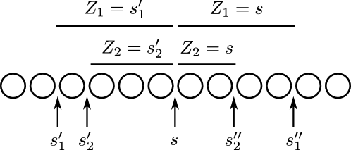
Figure 2: Illustration of boundaries used in proof of Theorem 3.

Let $s^{\prime}_{1}$ and $s^{\prime\prime}_{1}$ be the items right before and right after $s$ when we sort $S_{1}\cup\{s\}$. Also, let $Z_{1}$ and $Z^{\prime}_{1}$ be the random variables corresponding to $F(S_{1}\cup\{s\})$ and $F(S_{1})$ respectively. Similarly let $s^{\prime}_{2}$ and $s^{\prime\prime}_{2}$ be items right before and right after $s$ when we sort $S_{2}\cup\{s\}$, and let $Z_{2}$ and $Z^{\prime}_{2}$ be the random variables corresponding to $F(S_{2}\cup\{s\})$ and $F(S_{2})$ respectively.

Let us set $p_{1}=\Pr\left[Z_{1}=s^{\prime}_{1}\right]$, $q_{1}=\Pr\left[Z_{1}=s\right]$, $\alpha_{1}=\Pr\left[C=0|Z_{1}=s^{\prime}_{1}\right]$ and $\beta_{1}=\Pr\left[C=0|Z_{1}=s\right]$. Similarly let us set $p_{2}=\Pr\left[Z_{2}=s^{\prime}_{2}\right]$, $q_{2}=\Pr\left[Z_{2}=s\right]$, $\alpha_{2}=\Pr\left[C=0|Z_{2}=s^{\prime}_{2}\right]$ and $\beta_{2}=\Pr\left[C=0|Z_{2}=s\right]$. Note that since $S_{1}\subseteq S_{2}$, we have $s^{\prime}_{1},s^{\prime\prime}_{1}\in S_{2}$ and hence we have $s^{\prime}_{2}\geq s^{\prime}_{1}$ and $s^{\prime\prime}_{2}\leq s^{\prime\prime}_{1}$ (see Figure 2). Therefore, we have following set of inequalities

$$p_{2}=\Pr\left[Z_{2}=s^{\prime}_{2}\right] \leq\Pr\left[Z_{1}=s^{\prime}_{1}\right]=p_{1}\,,$$ (4)

$$q_{2}=\Pr\left[Z_{2}=s\right] \leq\Pr\left[Z_{1}=s\right]=q_{1}\,.$$ (5)

Since in the definition of $F(\cdot)$ the elements are ordered by $\Pr\left[C=0|X=x\right]$, we have the following set of inequalities

$$\alpha_{1}=\Pr\left[C=0|Z_{1}=s^{\prime}_{1}\right] \leq\Pr\left[C=0|Z_{1}=s\right]=\beta_{1}\,,$$ (6)

$$\alpha_{2}=\Pr\left[C=0|Z_{2}=s^{\prime}_{2}\right] \leq\Pr\left[C=0|Z_{2}=s\right]=\beta_{2}\,,$$ (7)

$$\alpha_{1}=\Pr\left[C=0|Z_{1}=s^{\prime}_{1}\right] \leq\Pr\left[C=0|Z_{2}=s^{\prime}_{2}\right]=\alpha_{2}\,,$$ (8)

$$\beta_{2}=\Pr\left[C=0|Z_{2}=s\right] \leq\Pr\left[C=0|Z_{1}=s\right]=\beta_{1}\,.$$ (9)

Finally, we have

$$\Delta_{s}F(S_{2})$$

$$\overset{(a)}{=}{} p_{2}f(\alpha_{2})+q_{2}f(\beta_{2})-(p_{2}+q_{2})f\big{(}\frac{p_{2}\alpha_{2}+q_{2}\beta_{2}}{p_{2}+q_{2}}\big{)}$$

$$\overset{(b)}{\leq}{} p_{2}f(\alpha_{2})+q_{2}f(\beta_{1})-(p_{2}+q_{2})f\big{(}\frac{p_{2}\alpha_{2}+q_{2}\beta_{1}}{p_{2}+q_{2}}\big{)}$$

$$\overset{(c)}{\leq}{} p_{2}f(\alpha_{1})+q_{2}f(\beta_{1})-(p_{2}+q_{2})f\big{(}\frac{p_{2}\alpha_{1}+q_{2}\beta_{1}}{p_{2}+q_{2}}\big{)}$$

$$\overset{(d)}{\leq}{} p_{1}f(\alpha_{1})+q_{2}f(\beta_{1})-(p_{1}+q_{2})f\big{(}\frac{p_{1}\alpha_{1}+q_{2}\beta_{1}}{p_{1}+q_{2}}\big{)}$$

$$\overset{(e)}{\leq}{} p_{1}f(\alpha_{1})+q_{1}f(\beta_{1})-(p_{1}+q_{1})f\big{(}\frac{p_{1}\alpha_{1}+q_{1}\beta_{1}}{p_{1}+q_{1}}\big{)}$$

$$\overset{(f)}{=}{} \Delta_{s}F(S_{1})\,,$$

where $(a)$ and $(f)$ follow from equality 2, $(b)$ follows from Corollary 1 and inequalities (9) and (7), $(c)$ follows from Corollary 2 and inequalities (8) and (6), $(d)$ follows from Lemma 3 and inequality (4), and $(e)$ follows from Lemma 3 and inequality (5). This completes the proof.  

2.3 Submodular Optimization Algorithms

Given that we have shown $F(\cdot)$ is submodular, we now show two approaches to optimization: a single machine algorithm that runs in time $O(n\log n)$ as well as an algorithm which allows the input to be processed in a distributed fashion, at the cost of an additional logarithmic factor in running time.

Single Machine Algorithm: We will make use of a $1-1/e-\epsilon$ approximation algorithm for submodular maximization that makes only $O(n)$ queries to $\Delta_{s}F(S)$ (Mirzasoleiman et al., 2015). First, fix an arbitrary small constant $\epsilon$ (this appears as a loss in the approximation factor as well as in the running time). The algorithm starts with an empty solution set and then proceeds in $m$ iterations where, in each iteration, we sample a set of $\frac{n\log{1/\epsilon}}{m}$ elements uniformly at random from the elements that have not been added to the solution so far and then add the sampled element with maximum marginal increase to the solution.

In general, we may expect that computing $\Delta_{s}F(S)$ requires at least $\Omega(|S|)$ time, which might be as large as $m$. However, we note that the algorithm of (Mirzasoleiman et al., 2015) (similar to most other algorithms for submodular maximization) only queries $\Delta_{s}F(S)$ for incrementally growing subsets of the final solution $S$. In that case, we can compute each incremental value of $\Delta_{s}F(S)$ in logarithmic time using a data structure that costs $O(n\log n)$ time to construct (see Algorithm  1). By using this query oracle, we do not require communicating the whole set $S$ for every query. Moreover, we use a red-black tree to maintain $S$, and hence we can search for neighbors ($s^{\prime}$ and $s^{\prime\prime}$) in logarithmic time. Thus, combining the submodular maximization algorithm that requires only a linear number of queries with the logarithmic time query oracle implies the following theorem.

Theorem 4

For any arbitrary small $\epsilon>0$, there exists a $(1-1/e-\epsilon)$-approximation algorithm for vocabulary compression that runs in $O(n\log n)$ time.

Procedure: Initialization
Input: Sorted list of probabilities $\Pr\left[C=0|X=x_{i}\right]$ and probabilities $\Pr\left[X=x_{i}\right]$.

1:  Initiate a red-black tree data structure $S$.

2:  Insert $0$ and $n$ into $S$.

3:  $p_{<0}\leftarrow 0$

4:  $p_{C=0|<0}\leftarrow 0$

5:  for $i=1$ to $n$ do

6:     $p_{<i}\leftarrow p_{<i-1}+\Pr\left[x=x_{i}\right]$

7:     $p_{C=0|<i}\leftarrow\frac{p_{C=0|<i-1}\times p_{<i-1}+\Pr\left[C=0|X=x_{i}\right]\times\Pr\left[x=x_{i}\right]}{p_{<i}}$.

8:  end for

Procedure: Query $\Delta_{s}F(S)$
Input: A number $s\in\{1,\dots,n-1\}\setminus S$

1:  $s^{\prime}\leftarrow$ largest element smaller than $s$ in $S$.

2:  $s^{\prime\prime}\leftarrow$ smallest element larger than $s$ in $S$.

3:  $p=p_{<s}-p_{<s^{\prime}}$

4:  $q=p_{<s^{\prime\prime}}-p_{<s}$

5:  $\alpha=\frac{p_{C=0|<s}\times p_{<s}-p_{C=0|<s^{\prime}}\times p_{<s^{\prime}}}{p}$

6:  $\beta=\frac{p_{C=0|<s^{\prime\prime}}\times p_{<s^{\prime\prime}}-p_{C=0|<s}\times p_{<s}}{q}$

7:  Return ${pf(\alpha)+qf(\beta)}-(p+q)f\big{(}\frac{p\alpha+q\beta}{p+q}\big{)}$ where $f(\cdot)$ is defined by equation (3).

Procedure: Insert $s$ to $S$
Input: A number $s\in\{1,\dots,n-1\}\setminus S$

1:  Insert $s$ into $S$.

Algorithm 1 Data structure to compute $\Delta_{s}F(S)$

Distributed Algorithm: Again, fix an arbitrary small number $\epsilon>0$ (for simplicity assume $\epsilon k$ and $\frac{n}{\epsilon k}$ are integers). In this distributed implementation we use $\epsilon k$ machines, requires $O(\frac{n}{\epsilon k})$ space per machine, and uses a logarithmic number of rounds of computation.

To define our distributed algorithm we start with the (non-distributed) submodular maximization algorithm of (Badanidiyuru and Vondrák, 2014), which provides a $1-1/e-\epsilon$ approximate solution using $O(n\log n)$ queries to the submodular function oracle. The algorithm works by defining a decreasing sequence of thresholds $w_{0},w_{1},\dots,w_{\log_{\frac{1}{1-\epsilon}}(n)}$, where $w_{0}$ is the maximum marginal increase of a single element, and $w_{i}=(1-\epsilon)^{i}w_{0}$. The algorithm proceeds in $\log_{\frac{1}{1-\epsilon}}(n)$ rounds, where in round $i$ the algorithm iterates over all elements and inserts an element $s$ into the solution set $S$ if $\Delta_{s}F(S)\geq w_{i}$. The algorithm stops once it has selected $k$ elements or if it finishes $\log_{\frac{1}{1-\epsilon}}(n)$ rounds, whichever comes first. As usual, this algorithm only queries $\Delta_{s}F(S)$ for incrementally growing subsets of the final solution $S$, and hence we can use Algorithm 1 to solve vocabulary compression in $O(n\log^{2}n)$ time.

Now, we show how to distribute this computation across multiple machines. First, for all $j\in\{1,\dots,\epsilon k-1\}$, we select the $(j\frac{n}{\epsilon k})$-th element and add it to the solution set $S$. This decomposes the elements into $\epsilon k$ continuous subsets of elements, each of size $\frac{n}{\epsilon k}$, and each of which we assign to one machine. Note that $\Delta_{s}F(S)$ only depends on the previous item and next item of $s$ in $S$ and, due to the way that we created the initial solution set $S$ and decomposed the input elements, the previous item and next item of $s$ are always both assigned to the same machine as $s$. Hence each machine can compute $\Delta_{s}F(S)$ locally. However, we assigned the first $\epsilon k-1$ to the solution set blindly and their marginal gain may be very small. Intuitively, we are potentially throwing away some of our selection budget for the ease of computation. Next we show that by forcing these elements into the solution we do not lose more than $\epsilon$ on the approximation factor.

First of all, notice that if we force a subset of the element to be included in the solution, the objective function is still submodular over the remaining elements. That is, the marginal impact of an element $s$ (i.e., $\Delta_{s}F(S)$) shrinks as $S$ grows. Next we show that if we force $\epsilon k-1$ elements into the solution, it does not decrease the value of the optimum solution by more than a $(1-\epsilon)$ factor. This means that if we provide a $(1-1/e-\epsilon)$-approximation to the new optimum solution, it is a $(1-\epsilon)\times(1-1/e-\epsilon)\leq(1-1/e-2\epsilon)$ approximate solution to the original optimum.

Let $S^{*}$ be a solution of size $k$ that maximizes $F(\cdot)$. Decompose $S^{*}$ into $\frac{1}{\epsilon}$ subsets of size $\epsilon k$. Note that by submodularity the value of $F(S^{*})$ is more than the sum of the marginal impacts of each $\frac{1}{\epsilon}$ subset (given the remainder of the subsets). Therefore, by the pigeonhole principle, the marginal impact of one of these subsets of $S^{*}$ is at most $\epsilon F(S^{*})$. If we remove this subset from $S^{*}$ and add the $\epsilon k-1$ forced elements, we find a solution of size (at most) $k$ that contains all of the forced elements and has value at least $(1-\epsilon)F(S^{*})$ as desired. Hence, by forcing these initial $\epsilon k-1$ elements to be in the solution we lose only an $\epsilon$ fraction on the approximation factor.

Now, to implement the algorithm of (Badanidiyuru and Vondrák, 2014), in iteration $i$, each machine independently finds and inserts all of its elements with marginal increase more than $w_{i}$. If the number of selected elements exceeds $k$, we remove the last few elements to have exactly $k$ elements in the solution. This implies the following theorem.

Theorem 5

For any arbitrary small $\epsilon>0$, there exists a $(1-1/e-\epsilon)$-approximation $(\log n)$-round distributed algorithm for vocabulary compression with $O(\frac{n}{k})$ space per machine and $O(n\log^{2}n)$ total work.

2.4 Heuristic Algorithms

In this subsection we review a couple of heuristics that can serve as simple alternatives to the algorithm we suggest and show that they can, in fact, fail entirely for some inputs. We also provide an empirical comparison to these, as well as the algorithm of Dhillon et al. (2003), in Section 3.

Bucketing Algorithm:

This algorithm splits the range of probabilities $[0,1]$ into $k$ equal size intervals $[0,1/k),[1/k,2/k),\dots,[(k-1)/k,1]$. Then it uses these intervals (or buckets) to form the compressed vocabulary. Specifically, each interval represents all elements $i$ such that $\Pr\left[C=0|X=i\right]\in[(j-1)/k,j/k)$. Note that there exists a set $S^{b}$ that such that $F(S^{b})$ correspond to the mutual information of the outcome of the bucketing algorithm and the labels. First we show that it is possible to give an upper bound on the mutual information loss, i.e., $I(X;C)-F(S^{b})$.

Theorem 6

Let $Z$ be the random variable provided by the bucketing algorithm. The total mutual information loss of the bucketing algorithm is bounded as follows.

$$I(X;C)-I(Z;C)\leq\Delta_{\max},$$

where $\Delta_{\max}=\max_{j}\big{(}\max_{r\in[(j-1)/k,j/k)}f(r)-\min_{r\in[\frac{j-1}{k},\frac{j}{k})}f(r)\big{)}$ and $f(\cdot)$ is defined in equation (3).

Proof Note that as we showed in Subsection 2.2 we have

$$F(S) =\sum_{z\sim Z}\Pr\left[Z=z\right]f(\Pr\left[C=0|Z=z\right])$$

$$=\sum_{z\sim Z}\Pr\left[Z=z\right]f\Big{(}E_{x\in z}\big{[}\Pr\left[C=0|X=x\right]\big{]}\Big{)}.$$ (10)

On the other hand we have

$$I(X;C)=\sum_{x\sim X}\Pr\left[X=x\right]f(\Pr\left[C=0|X=x\right])$$

$$= \sum_{z\sim Z}\sum_{x\in z}\Pr\left[X=x\right]f(\Pr\left[C=0|X=x\right])$$

$$= \sum_{z\sim Z}\Pr\left[Z=z\right]\sum_{x\in z}\frac{\Pr\left[X=x\right]}{\Pr\left[Z=z\right]}f(\Pr\left[C=0|X=x\right])$$

$$= \sum_{z\sim Z}\Pr\left[Z=z\right]E_{x\in z}\Big{[}f\big{(}\Pr\left[C=0|X=x\right]\big{)}\Big{]}.$$ (11)

Let $j$ be the index of the interval corresponding to $z$. Then, by convexity of $f(\cdot)$, we have

$$E_{x\in z}\big{[}f\big{(}\Pr\left[C=0|X=x\right]\big{)}\big{]}\leq\max_{r\in[\frac{j-1}{k},\frac{j}{k})}f(r)$$

and

$$f\big{(}E_{x\in z}\big{[}\Pr\left[C=0|X=x\right]\big{]}\big{)}\geq\min_{r\in[\frac{j-1}{k},\frac{j}{k})}f(r)\,.$$

Therefore we have

$$E_{x\in z}\Big{[}f\big{(}\Pr\left[C=0|X=x\right]\big{)}\Big{]}-f\Big{(}E_{x\in z}\big{[}\Pr\left[C=0|X=x\right]\big{]}\Big{)}\\ \leq\max_{r\in[(j-1)/k,j/k)}f(r)-\min_{r\in[(j-1)/k,j/k)}f(r)\leq\Delta_{\max}\,.$$

This together with Equations (2.4) and (11) show that $I(X;C)-F(S)\leq\sum_{z\sim Z}\Pr\left[Z=z\right]\Delta_{\max}=\Delta_{\max}$ and completes the theorem.  
The above theorem states that the information loss of the bucketing algorithm is no more than how much $f(\cdot)$ changes within one interval of size $1/k$. Note that this is an absolute loss and is not comparable to the approximation guarantee that we provide submodular maximization. The main problem with the bucketing algorithm is that it is to some extent oblivious to the input data and, thus, will fail badly for certain inputs as shown in the following proposition.

Proposition 7

There is an input $X$ to the bucketing algorithm such that $I(X;C)>0$ and $I(Z;C)=0$, where $Z$ is the output of the bucketing algorithm.

Proof Fix a number $j$. In this example for half of the items we have $\Pr\left[C=0|X=x\right]=\frac{j+1/3}{k}$ and for the other half we have $\Pr\left[C=0|X=x\right]=\frac{j+2/3}{k}$. We also set the probability of all values of $X$ to be the same, and hence $\Pr\left[C=0\right]=\frac{j+0.5}{k}$. The mutual information of $X$ with the label is non-zero since $\Pr\left[C=0\right]\neq\Pr\left[C=0|X=x\right]$. However, the bucketing algorithm merges all of the elements in the range $[\frac{j}{k},\frac{j+1}{k})$, thereby merging all values together giving us $I(Z;C)=0$ and completing the proof.  
Note, we can further strengthen the previous example by giving a tiny mass to all buckets, so that all values do not collapse into a single bucket. However, still in this case, the bucketing method can only hope to capture a tiny fraction of mutual information since the vast majority of mass falls into a single bucket.

Frequency Based Filtering:

This is very simple compression method (more precisely, a feature selection method) that is popular in practice. Given a vocabulary budget, we compute a frequency threshold $\tau$ which we use to remove any vocabulary value that appears in fewer than $\tau$ instances of our dataset and which results in a vocabulary of the desired size. Even though the frequency based algorithm is not entirely oblivious to the input, it is oblivious to the label and hence oblivious to conditional distributions. Similar to the bucketing algorithm with a simple example in the following theorem we show that the frequency based algorithm fails to provide any approximation gaurantee.

Proposition 8

There is an input $X$ to the frequency based algorithm such that $I(X;C)>0$ and $I(Z;C)=0$, where $Z$ is the outcome of the frequency based algorithm.

Proof Assume we have $n=3k$ values for $X$, namely $x_{1},\dots,x_{n}$. For all $i\in\{1,\dots,k\}$ define $\Pr\left[X=x_{i}\right]=2/n$, and for all $i\in\{k+1,\dots,n\}$ we have $\Pr\left[X=x_{i}\right]=0.5/n$. Note that the first $k$ values are the most frequent values, however, we are going to define them such that they are independent of the label.

For $\forall i\in\{1,\dots,k\}$ let $\Pr\left[X=x_{i}|C=0\right]=1/2$; for $\forall i\in\{k+1,\dots,2k\}$ let $\Pr\left[X=x_{i}|C=0\right]=0$; and for $\forall i\in\{2k+1,\dots,3k\}$ let $\Pr\left[X=x_{i}|C=0\right]=1$. Note that we have $\Pr\left[C=0\right]=\frac{1}{2}$. Therefore the mutual information of the $k$ most frequent values with the label is zero, which implies for a certain vocabulary budget, and thereby frequency threshold, $I(Z;C)=0$. Observe that even if we merge the last $2k$ values and use it as a new value (as opposed to ignoring them), the label corresponding the the merged value is $0$ with probability half, and hence has no mutual information with the label. However, we have $I(X;C)=\sum_{x\sim X}\Pr\left[X=x\right]f(\Pr\left[C=0|X=x\right])=\sum_{i=k+1}^{2k}\frac{0.5}{n}=\frac{0.5\times 2k}{3k}=\frac{1}{3}>0$, which completes the proof.  

3 Empirical Evaluation

In this section we report our empirical evaluation of the optimization the submodular function $F(S)$ described in the previous section. All the experiments are performed using the Criteo click prediction dataset (CriteoLabs, 2014), which consists of 37 million instances for training and 4.4 million held-out points. In addition to 13 numerical features, this dataset contains 26 categorical features with a combined total vocabulary of more than 28 million values. These features have varying vocabulary sizes, from a handful up to millions of values. Five features, in particular, have more than a million distinct feature values each.

In order to execute a mutual information based algorithm, we require estimates of the conditional probabilities $\Pr\left[C=0|X=x_{i}\right]$ and marginal probabilities $\Pr\left[X=x_{i}\right]$. Here, we simply use the maximum likelihood estimate based on the empirical count, i.e. given a sample of feature value and label pairs $\big{(}(\hat{x}_{1},\hat{c}_{1}),\ldots,(\hat{x}_{k},\hat{c}_{k})\big{)}$, we have

We note that such estimates may sometimes be poor, especially when certain feature values appear very rarely. Evaluating more robust estimates is outside the scope of the current study, but an interesting direction for future work.

3.1 Mutual information evaluation

We first evaluate the ability of our algorithm to maximize the mutual information retained by the compressed vocabulary and compare it to other baseline methods.

In particular, we compare our algorithm to the iterative divisive clustering algorithm introduced by Dhillon et al. (2003), as well as the frequency filtering and bucketing heuristics introduced in the previous section. The divisive clustering algorithm resembles a version of the $k$-means algorithm where $k$ is set to be the vocabulary size and distances between points and clusters are defined in terms of the KL divergence between the conditional distribution of the label variable given a feature value and the conditional distribution of the label variable given a cluster center. Notice that due to the large size of the dataset, we cannot run the dynamic programming algorithm introduced by Kurkoski and Yagi (2014) which would find the theoretically optimal solution. For ease of reference, we call our algorithm Submodular, and the other algorithms Divisive, Bucketing and Frequency.

Note that our algorithm, as well as previous algorithms, seek to maximize the mutual information between a single categorical variable and the label, while in the Criteo dataset we have several categorical variables that we wish to apply a global vocabulary size budget to. In the case of the Frequency heuristic, this issue is addressed by sorting the counts of feature values across all categorical variables and applying a global threshold. In the case of Submodular, we run the almost linear-time algorithm for each categorical variable to obtain a sorted list of feature values and their marginal contributions to the global objective. Then we sort these marginal values and pick the top-score feature values to obtain the desired target vocabulary size. Thus, both Submodular and Frequency are able to naturally employ global strategies in order to allocate the total vocabulary budget across different categorical features.

For the Divisive and Bucketing algorithms, a natural global allocation policy is not available, as one needs to define an allocation of the vocabulary budget to each categorical feature a priori. In this study, we evaluate two natural allocation mechanisms. The uniform allocation assigns a uniform budget across all categorical features, whereas the MI allocation assigns a budget that is proportional to the mutual information of the particular categorical feature.

The original vocabulary of over 28 million values is compressed by a factor of up to 2000. Using the methods mentioned above, we obtain vocabularies of size 10K, 20K, 40K, 80K, 120K and 160K. Then we compute the loss in average mutual information, which is defined as follows: let $X_{i}$ denote the mutual information of uncompressed categorical feature $i$ with the label and $Z_{i}$ denote mutual information of the corresponding compressed feature, then the average mutual information loss is equal to $(\sum_{i}X_{i}-Z_{i})/(\sum_{j}X_{j})$.

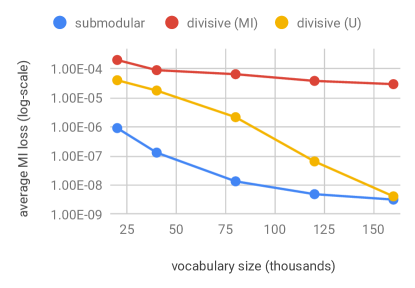
Figure 3: The average mutual information loss of several compression methods measured on to the Criteo dataset.

For the heuristic Frequency algorithm, the measured loss ranges from 0.520 (for budget of 160K) to 0.654 (for budget of 10K), while for Bucketing the loss ranges from $5\times 10^{-6}$ to $5\times 10^{-3}$. As expected, the mutual information based methods perform significantly better, in particular, the loss for Submodular ranges from $9\times 10^{-7}$ to $3\times 10^{-9}$ and consistently outperforms the Divisive algorithm (regardless of allocation strategy). Figure 3 provides a closer look at the mutual information based methods. Thus, we find that not only is our method fast, scalable and exhibits a theoretical $1-1/e$ lower bound on the performance, but that in practice it maintains almost all the mutual information between data points and the labels.

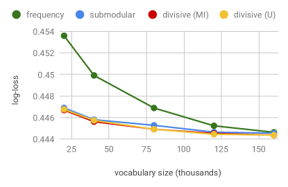
Figure 4: The log-loss of a neural network model trained with compressed vocabularies of several sizes and using several different compression methods.

3.2 Learning evaluation

Our focus thus far has been in optimizing the mutual information objective. In this section we also evaluate the compressed vocabularies in an end-to-end task to demonstrate its application in a learning scenario.

Given a compressed vocabulary we train a neural network model on the training split and measure the log-loss on the hold out set (futher details in supplement Section A.2). In Figure 4 we see that the mutual information based methods perform comparably to each other and significantly outperform popular heuristic method Frequency. We observe that our scalable quasi-linear compression algorithm with provable approximation guarantees also performs competitively in end-to-end learning.

4 Conclusion

In this work we have shown the first scalable quasi-linear compression algorithm for maximizing mutual information with the label that also exhibits and $1-1/e$ factor approximation guarantee. The algorithm, as well as our insights into constructing a submodular objective function, might be of interest in other applications as well (for example, quantization in DMC). One future line of work is extending this work to the multiclass (non-binary) setting.

A Supplement

A.1 Proof of technical lemmas

Proof of Lemma 1  Let $Z$ and $Z^{\prime}$ be the random variables corresponding to $F(S\cup\{s\})$ and $F(S)$ respectively. Note that we have

$$F(S) =\sum_{z^{\prime}\sim Z^{\prime}}\sum_{c\in\{0,1\}}\Pr\left[Z^{\prime}=z^{\prime},C=c\right]\log\frac{\Pr\left[Z^{\prime}=z^{\prime},C=c\right]}{\Pr\left[Z^{\prime}=z^{\prime}\right]\Pr\left[C=c\right]}$$

$$=\sum_{z^{\prime}\sim Z^{\prime}}\Pr\left[Z^{\prime}=z^{\prime}\right]\sum_{c\in\{0,1\}}\Pr\left[C=c|Z^{\prime}=z^{\prime}\right]\log\frac{\Pr\left[C=c|Z^{\prime}=z^{\prime}\right]}{\Pr\left[C=c\right]}$$

$$=\sum_{z^{\prime}\sim Z^{\prime}}\Pr\left[Z^{\prime}=z^{\prime}\right]f(\Pr\left[C=0|Z^{\prime}=z^{\prime}\right]),$$

where we have

$$f(t)=t\log\frac{t}{\Pr\left[C=0\right]}+(1-t)\log\frac{1-t}{\Pr\left[C=1\right]}\,,$$

which is a convex function over $t\in[0,1]$. Next, we have

$$\Delta_{s}F(S)={} F(S\cup\{s\})-F(S)$$

$$={} \sum_{z\sim Z}\Pr\left[Z=z\right]f(\Pr\left[C=0|Z=z\right])-\sum_{z^{\prime}\sim Z^{\prime}}\Pr\left[Z^{\prime}=z^{\prime}\right]f(\Pr\left[C=0|Z^{\prime}=z^{\prime}\right])$$

$$={} \Pr\left[Z=s^{\prime}\right]f(\Pr\left[C=0|Z=s^{\prime}\right])+\Pr\left[Z=s\right]f(\Pr\left[C=0|Z=s\right])$$

$$-\Pr\left[Z^{\prime}=s^{\prime}\right]f(\Pr\left[C=0|Z^{\prime}=s^{\prime}\right]).$$

Notice that $Z^{\prime}=s^{\prime}$ implies that $Z=s$ or $Z=s^{\prime}$. Hence we have $\Pr\left[Z^{\prime}=s^{\prime}\right]=\Pr\left[Z=s^{\prime}\right]+\Pr\left[Z=s\right]$ and

$$\Pr\left[C=0|Z^{\prime}=s^{\prime}\right]=\frac{\Pr\left[Z=s^{\prime}\right]\Pr\left[C=0|Z=s^{\prime}\right]+\Pr\left[Z=s\right]\Pr\left[C=0|Z=s\right]}{\Pr\left[Z=s^{\prime}\right]+\Pr\left[Z=s\right]}\,.$$

Now, if we set $p=\Pr\left[Z=s^{\prime}\right]$, $q=\Pr\left[Z=s\right]$, $\alpha=\Pr\left[C=0|Z=s^{\prime}\right]$ and $\beta=\Pr\left[C=0|Z=s\right]$, and combine the previous two inline equalities, we have

$$\Delta_{s}F(S)={pf(\alpha)+qf(\beta)}-(p+q)f\big{(}\frac{p\alpha+q\beta}{p+q}\big{)}\,.$$

 

Some Basic Tools: In Lemmas 2 and 3 we show two basic properties of convex functions that later become handy in our proof. We use the following property of convex functions to prove Lemma 2. For any convex function $f$ and any three numbers $a<b<c$ we have

$$\frac{f(b)-f(a)}{b-a}\leq\frac{f(c)-f(b)}{c-b}.$$ (12)

Note that this also implies

$$\frac{f(c)-f(a)}{c-a} =\frac{1}{c-a}\big{(}f(c)-f(b)+f(b)-f(a)\big{)}$$

$$\leq\frac{1}{c-a}\Big{(}f(c)-f(b)+\frac{b-a}{c-b}\big{(}f(c)-f(b)\big{)}\Big{)}$$ By Inequality 12

$$=\frac{1}{c-a}\Big{(}\frac{c-b+b-a}{c-b}\big{(}f(c)-f(b)\big{)}\Big{)}$$

$$=\frac{f(c)-f(b)}{c-b}.$$ (13)

Similarly we have

$$\frac{f(c)-f(a)}{c-a} =\frac{1}{c-a}\big{(}f(c)-f(b)+f(b)-f(a)\big{)}$$

$$\geq\frac{1}{c-a}\Big{(}\frac{c-b}{b-a}\big{(}f(b)-f(a)\big{)}+f(b)-f(a)\Big{)}$$ By Inequality 12

$$\geq\frac{1}{c-a}\Big{(}\frac{c-b+b-a}{b-a}\big{(}f(b)-f(a)\big{)}\Big{)}$$

$$=\frac{f(b)-f(a)}{b-a}.$$ (14)

Proof of Lemma 2  First, we prove

$$\frac{f(p\alpha+q\gamma)-f(p\alpha+q\beta)}{q\gamma-q\beta}\leq\frac{f(\gamma)-f(\beta)}{\gamma-\beta}.$$ (15)

Recall that $\alpha\leq\beta\leq\gamma$, and $p+q=1$. Hence we have $p\alpha+q\beta\leq p\alpha+q\gamma,\beta\leq\gamma$. We prove Inequality 15 in two cases of $p\alpha+q\gamma\leq\beta$, and $\beta<p\alpha+q\gamma$. Case 1. In this case we have $p\alpha+q\beta\leq p\alpha+q\gamma\leq\beta\leq\gamma$. we have

$$\frac{f(p\alpha+q\gamma)-f(p\alpha+q\beta)}{q\gamma-q\beta} =\frac{f(p\alpha+q\gamma)-f(p\alpha+q\beta)}{(p\alpha+q\gamma)-(p\alpha+q\beta)}$$

$$\leq\frac{f(\beta)-f(p\alpha+q\gamma)}{\beta-(p\alpha+q\gamma)}$$ By Inequality 12

$$\leq\frac{f(\gamma)-f(\beta)}{\gamma-\beta}$$ By Inequality 12

Case 2. In this case we have $p\alpha+q\beta\leq\beta\leq p\alpha+q\gamma\leq\gamma$. we have

$$\frac{f(p\alpha+q\gamma)-f(p\alpha+q\beta)}{q\gamma-q\beta} =\frac{f(p\alpha+q\gamma)-f(p\alpha+q\beta)}{(p\alpha+q\gamma)-(p\alpha+q\beta)}$$

$$\leq\frac{f(p\alpha+q\gamma)-f(\beta)}{(p\alpha+q\gamma)-\beta}$$ By Inequality A.1

$$\leq\frac{f(\gamma)-f(\beta)}{\gamma-\beta} \text{By Inequality \ref{eq:convexDef3}}.$$

Next we use Inequality 15 to prove the lemma. By multiplying both sides of Inequality 15 by $q(\gamma-\beta)$ we have

$${f(p\alpha+q\gamma)-f(p\alpha+q\beta)}\leq{qf(\gamma)-qf(\beta)}.$$

By rearranging the terms and adding $pf(\alpha)$ to both sides we have

$$\big{(}pf(\alpha)+qf(\beta)\big{)}-f(p\alpha+q\beta)\leq\big{(}pf(\alpha)+qf(\gamma)\big{)}-f(p\alpha+q\gamma),$$

as desired.  

Proof of Lemma 3  We have

$$\frac{p+q}{p+q^{\prime}}f\big{(}\frac{p\alpha+q\beta}{p+q}\big{)}+\frac{q^{\prime}-q}{p+q^{\prime}}f(\beta) \geq f\big{(}\frac{p+q}{p+q^{\prime}}\frac{p\alpha+q\beta}{p+q}+\frac{q^{\prime}-q}{p+q^{\prime}}\beta\big{)}$$ By convexity

$$=f\big{(}\frac{p\alpha+q\beta}{p+q^{\prime}}+\frac{q^{\prime}-q}{p+q^{\prime}}\beta\big{)}$$

$$=f\big{(}\frac{p\alpha+q^{\prime}\beta}{p+q^{\prime}}\big{)}.$$

By multiplying both sides by $p+q^{\prime}$ we have

$$(p+q)f\big{(}\frac{p\alpha+q\beta}{p+q}\big{)}+q^{\prime}f(\beta)-qf(\beta) \geq(p+q^{\prime})f\big{(}\frac{p\alpha+q^{\prime}\beta}{p+q^{\prime}}\big{)}.$$

By rearranging the terms and adding $pf(\alpha)$ to both sides we have

$$pf(\alpha)+qf(\beta)-(p+q)f\big{(}\frac{p\alpha+q\beta}{p+q}\big{)}\leq pf(\alpha)+q^{\prime}f(\beta)-(p+q^{\prime})f\big{(}\frac{p\alpha+q^{\prime}\beta}{p+q^{\prime}}\big{)},$$

as desired.  

A.2 Empirical Evaluation Details

We implement the neural network using TensorFlow and train it using the AdamOptimizer [Abadi et al., 2016, Kingma and Ba, 2014]. The following set of neural network hyperparameters are tuned by evaluating 2000 different configurations on the hold-out set as suggested by a Gaussian Process black-box optimization routine.

hyperparameter	search range
hidden layer size	[100, 1280]
num hidden layers	[1, 5]
learning rate	[1e-6, 0.01]
gradient clip norm	[1.0, 1000.0]
$L_{2}$-regularization	[0, 1e-4]

References

- Abadi et al. [2016] Martín Abadi, Paul Barham, Jianmin Chen, Zhifeng Chen, Andy Davis, Jeffrey Dean, Matthieu Devin, Sanjay Ghemawat, Geoffrey Irving, Michael Isard, et al. Tensorflow: a system for large-scale machine learning. In OSDI, volume 16, pages 265–283, 2016.
- Aggarwal et al. [1987] Alok Aggarwal, Maria M Klawe, Shlomo Moran, Peter Shor, and Robert Wilber. Geometric applications of a matrix-searching algorithm. Algorithmica, 2(1-4):195–208, 1987.
- Badanidiyuru and Vondrák [2014] Ashwinkumar Badanidiyuru and Jan Vondrák. Fast algorithms for maximizing submodular functions. In Proceedings of the twenty-fifth annual ACM-SIAM symposium on Discrete algorithms, pages 1497–1514. SIAM, 2014.
- Baker and McCallum [1998] L Douglas Baker and Andrew Kachites McCallum. Distributional clustering of words for text classification. In Proceedings of the 21st annual international ACM SIGIR conference on Research and development in information retrieval, pages 96–103. ACM, 1998.
- Barbosa et al. [2015] Rafael Barbosa, Alina Ene, Huy Nguyen, and Justin Ward. The power of randomization: Distributed submodular maximization on massive datasets. In International Conference on Machine Learning, pages 1236–1244, 2015.
- Cicalese et al. [2018] Ferdinando Cicalese, Luisa Gargano, and Ugo Vaccaro. Bounds on the entropy of a function of a random variable and their applications. IEEE Transactions on Information Theory, 64(4):2220–2230, 2018.
- Cover and Thomas [2006] Thomas M. Cover and Joy A. Thomas. Elements of Information Theory (Wiley Series in Telecommunications and Signal Processing). Wiley-Interscience, New York, NY, USA, 2006.
- CriteoLabs [2014] CriteoLabs. Display Advertising Challenge, 2014. URL https://www.kaggle.com/c/criteo-display-ad-challenge.
- Dhillon et al. [2003] Inderjit S Dhillon, Subramanyam Mallela, and Rahul Kumar. A divisive information-theoretic feature clustering algorithm for text classification. Journal of machine learning research, 3(Mar):1265–1287, 2003.
- Guyon and Elisseeff [2003] Isabelle Guyon and André Elisseeff. An introduction to variable and feature selection. Journal of machine learning research, 3(Mar):1157–1182, 2003.
- Iwata and Ozawa [2014] Ken-ichi Iwata and Shin-ya Ozawa. Quantizer design for outputs of binary-input discrete memoryless channels using smawk algorithm. In Information Theory (ISIT), 2014 IEEE International Symposium on, pages 191–195. IEEE, 2014.
- Jiang et al. [2011] Jung-Yi Jiang, Ren-Jia Liou, and Shie-Jue Lee. A fuzzy self-constructing feature clustering algorithm for text classification. IEEE transactions on knowledge and data engineering, 23(3):335–349, 2011.
- Kingma and Ba [2014] Diederik P Kingma and Jimmy Ba. Adam: A method for stochastic optimization. arXiv preprint arXiv:1412.6980, 2014.
- Kumar et al. [2015] Ravi Kumar, Benjamin Moseley, Sergei Vassilvitskii, and Andrea Vattani. Fast greedy algorithms in mapreduce and streaming. ACM Transactions on Parallel Computing (TOPC), 2(3):14, 2015.
- Kurkoski and Yagi [2014] Brian M Kurkoski and Hideki Yagi. Quantization of binary-input discrete memoryless channels. IEEE Transactions on Information Theory, 60(8):4544–4552, 2014.
- Mirrokni and Zadimoghaddam [2015] Vahab Mirrokni and Morteza Zadimoghaddam. Randomized composable core-sets for distributed submodular maximization. In Proceedings of the forty-seventh annual ACM symposium on Theory of computing, pages 153–162. ACM, 2015.
- Mirzasoleiman et al. [2013] Baharan Mirzasoleiman, Amin Karbasi, Rik Sarkar, and Andreas Krause. Distributed submodular maximization: Identifying representative elements in massive data. In Advances in Neural Information Processing Systems, pages 2049–2057, 2013.
- Mirzasoleiman et al. [2015] Baharan Mirzasoleiman, Ashwinkumar Badanidiyuru, Amin Karbasi, Jan Vondrák, and Andreas Krause. Lazier than lazy greedy. In AAAI, pages 1812–1818, 2015.
- Mohri et al. [2018] Mehryar Mohri, Afshin Rostamizadeh, and Ameet Talwalkar. Foundations of machine learning. MIT press, 2018.
- Mumey and Gedeon [2003] Brendan Mumey and Tomáš Gedeon. Optimal mutual information quantization is np-complete. In Proc. Neural Inf. Coding (NIC) Workshop, 2003.
- Slonim and Tishby [2001] Noam Slonim and Naftali Tishby. The power of word clusters for text classification. In 23rd European Colloquium on Information Retrieval Research, volume 1, page 200, 2001.
- Zhang and Kurkoski [2016] Jiuyang Alan Zhang and Brian M Kurkoski. Low-complexity quantization of discrete memoryless channels. In Information Theory and Its Applications (ISITA), 2016 International Symposium on, pages 448–452. IEEE, 2016.