Constraints on the redshift evolution of astrophysical feedback with Sunyaev-Zel’dovich effect cross-correlations

Abstract

An understanding of astrophysical feedback is important for constraining models of galaxy formation and for extracting cosmological information from current and future weak lensing surveys. The thermal Sunyaev-Zel’dovich effect, quantified via the Compton-$y$ parameter, is a powerful tool for studying feedback, because it directly probes the pressure of the hot, ionized gas residing in dark matter halos. Cross-correlations between galaxies and maps of Compton-$y$ obtained from cosmic microwave background surveys are sensitive to the redshift evolution of the gas pressure, and its dependence on halo mass. In this work, we use galaxies identified in year one data from the Dark Energy Survey and Compton-$y$ maps constructed from Planck observations. We find highly significant (roughly $12\sigma$) detections of galaxy-$y$ cross-correlation in multiple redshift bins. By jointly fitting these measurements as well as measurements of galaxy clustering, we constrain the halo bias-weighted, gas pressure of the Universe as a function of redshift between $0.15\lesssim z\lesssim 0.75$. We compare these measurements to predictions from hydrodynamical simulations, allowing us to constrain the amount of thermal energy in the halo gas relative to that resulting from gravitational collapse.

I Introduction

The nonlinear collapse of structure at late times leads to the formation of gravitationally bound dark matter halos. These massive objects are reservoirs of hot gas, with virial temperatures as high as $T\sim 10^{8}\,{\rm K}$. This gas can be studied via its thermal emission, which is typically peaked in x-ray bands (for a review, see e.g. Böhringer & Werner, 2010). Another way to study the gas in halos is via the thermal Sunyaev-Zel’dovich (tSZ) effect (Sunyaev & Zeldovich, 1972), caused by inverse Compton scattering of CMB photons with the hot gas. This scattering process leads to a spectral distortion which is observable at millimeter wavelengths (e.g. Carlstrom et al., 2002).

The amplitude of the tSZ effect in some direction on the sky is characterized by the Compton-$y$ parameter, which is related to an integral along the line of sight of the ionized gas pressure. By measuring contributions to $y$ as a function of redshift, we effectively probe the evolution of the gas pressure over cosmic time. For the most massive halos, the evolution of the gas pressure is expected to be dominated by gravitational physics. Gas falling into these halos is shock heated to the virial temperature during infall into the cluster potential (Evrard, 1990). For lower mass halos, on the other hand, other mechanisms may deposit energy and/or momentum into the gas; these mechanisms are generically referred to as "feedback."

An understanding of baryonic feedback is important for constraining models of galaxy formation (for a recent review, see Naab & Ostriker, 2017). Furthermore, since feedback can redistribute mass around halos (e.g. via gas outflows), an understanding of these processes is necessary for extracting cosmological constraints from small-scale measurements of the matter power spectrum with e.g. weak lensing surveys (Rudd et al., 2008; van Daalen et al., 2011).

Because $y$ is sensitive to the line-of-sight integrated gas pressure, measurements of $y$ alone (such as the $y$ power spectrum) cannot be used to to directly determine the redshift evolution of the gas pressure. However, given some tracer of the matter density field which can be restricted to narrow redshift intervals, cross-correlations of this tracer with $y$ can be used to isolate contributions to $y$ from different redshifts. We take the cross-correlation approach in this analysis.

By cross-correlating a sample of galaxies identified in data from the Dark Energy Survey (DES) (Flaugher et al., 2015) with $y$ maps generated from Planck data (Aghanim et al., 2015), we measure the evolution of the gas pressure as a function of redshift. As we discuss in §II, our cross-correlation measurements are sensitive to a combination of the gas pressure and the amplitude of galaxy clustering. To break this degeneracy, we perform a joint fit to measurements of the galaxy-$y$ cross-correlation and to galaxy-galaxy clustering to constrain both the redshift evolution of the galaxy bias, and the redshift evolution of a term depending on the average gas pressure in dark matter halos.

Our analysis relies on the so-called redMaGiC galaxy selection from DES. The redMaGiC algorithm yields a sample of galaxies whose photometric redshifts are well constrained (Rozo et al., 2016). We note that we do not attempt to model the halo-galaxy connection for the redMaGiC galaxies. Rather, we use these galaxies only as tracers of the density field for the purposes of isolating contributions to $y$ from different redshifts. Consequently, we will restrict our measurements to the two-halo regime, for which the galaxy-$y$ cross-correlation can be modeled without dependence on the precise way that redMaGiC galaxies populate halos (for a review of the halo model see Cooray & Sheth, 2002).

Several previous analyses have also considered the cross-correlation between galaxy catalogs and Compton-$y$ maps from Planck (Vikram et al., 2017; Hill et al., 2018; Makiya et al., 2018; Tanimura et al., 2019). Vikram et al. (2017) (hereafter V17) correlated Planck $y$ maps with a sample of galaxy groups identified from Sloan Digital Sky Survey (SDSS) data by Yang et al. (2007). Our analysis differs from that of V17 in several important respects. First, the galaxy sample used in this analysis is derived from DES data, and extends to significantly higher redshift ($z\sim 0.7$) than considered by V17 ($z\lesssim 0.2$). Additionally, while V17 divided their correlation measurements into bins of halo mass, we divide our measurements into bins of halo redshift. The measurements presented here can be considered complementary to those of V17 with regard to constraining feedback models.

Hill et al. (2018) used measurements and modeling similar to V17 in order to extract constraints on the halo $Y$-$M$ relation, finding hints of departure from the predictions of self-similar models at low halo masses. Our approach is similar to that of Hill et al. (2018), although we only fit measurements in the two-halo regime.

Planck Collaboration et al. (2013) correlated galaxies identified in SDSS data with Planck $y$ maps. The galaxy catalog used by Planck Collaboration et al. (2013) was restricted to "isolated" galaxies in order to probe the pressure profiles of individual small mass halos (although note the issues with this approach pointed out by Le Brun et al. (2015), Greco et al. (2015) and Hill et al. (2018)). Several authors have also investigated related correlations between Compton-$y$ and weak lensing (Van Waerbeke et al., 2014; Hill & Spergel, 2013) .

Recently, Tanimura et al. (2019) measured the correlation of luminous red galaxies (LRGs) with the Planck $y$ maps in order to study astrophysical feedback. Our analysis differs from that of Tanimura et al. (2019) in two crucial aspects. First, we are only interested in the galaxy-$y$ cross-correlations in the two-halo regime, whereas Tanimura et al. (2019) analyzed the full $y$ profile around LRGs, including in the one-halo regime. Second, and more importantly, the quantity of interest in the present work, namely the bias weighted pressure of the universe, is not sensitive to the connection between the galaxies used for cross-correlations and the parent halo, nor to the properties of the galaxies. The analysis of Tanimura et al. (2019) exhibits strong dependence on the connection between stellar mass and halo mass for their LRG sample.

The structure of the paper is as follows. In §II we present our model for the galaxy-$y$ and galaxy-galaxy cross-correlation measurements; in §III we describe the DES, Planck and simulation data sets used in our analysis; in §IV we describe our measurement and fitting procedure, and validate this procedure by applying it to simulations; in §V we present the results of our analysis applied to the data. We conclude in §VI.

II Formalism

We are interested in modeling both the galaxy-$y$ and galaxy-galaxy correlation functions to extract constraints on the redshift evolution of the gas pressure. Our analysis will focus on the large-scale, two-halo regime in which the details of the galaxy-halo connection can be ignored. The primary motivation for this choice is that in the two-halo regime, the galaxy-$y$ cross-correlation function is insensitive to the details of the galaxy-halo connection, significantly simplifying the analysis.

We will assume a fixed $\Lambda$CDM cosmological model throughout, and will therefore suppress dependence on cosmological parameters. When analyzing the data, we adopt a $\Lambda$CDM model with $h=0.7$, $\Omega_{\rm m}=0.28$, $\Omega_{b}=0.044$, $n_{s}=0.965$ and $\sigma_{8}=0.8$. Given the uncertainties on our measurement of the galaxy-$y$ cross-correlation, adopting instead the best-fit cosmology from e.g. Planck Collaboration et al. (2018) has a negligible impact on our main constraints.

II.1 Model for galaxy-$y$ cross-correlation

The observed temperature signal on the sky in the direction $\hat{n}$ and at frequency $\nu$ due to the tSZ effect can be written as

$$\Delta T(\hat{n},\nu)=T_{\rm CMB}y(\hat{n})f(\nu),$$ (1)

where $T_{\rm CMB}=2.73\,{\rm K}$ is the mean temperature of the CMB, and $y(\hat{n})$ is the Compton-$y$ parameter. In the non-relativistic limit, we have (Sunyaev & Zeldovich, 1980):

$$f(x=h\nu/k_{B}T_{\rm CMB})=x\frac{e^{x}+1}{e^{x}-1}-4,$$ (2)

where $h$ is Planck’s constant, and $k_{B}$ is the Boltzmann constant.

The Compton-$y$ parameter is in turn given by (suppressing the directional dependence):

$$y=\frac{\sigma_{T}}{m_{e}c^{2}}\int_{0}^{\infty}dl\,P_{e}(l),$$ (3)

where $P_{e}(l)$ is the electron gas pressure (which dominates the inverse Compton scattering process that gives rise to the tSZ effect) at line of sight distance $l$, $\sigma_{T}$ is the Thomson cross section, $m_{e}$ is the electron mass and $c$ is the speed of light. For a fully ionized gas consisting of hydrogen and helium, the electron pressure, $P_{e}$, is related to the total thermal pressure, $P_{th}$, by:

$$P_{e}=\left[\frac{4-2Y}{8-5Y}\right]P_{th},$$ (4)

where $Y$ is the primordial helium mass fraction. We adopt $Y=0.24$.

We denote the galaxy-$y$ cross-correlation with $\xi_{yg}(R)$. This quantity represents the expectation value of $y$ at transverse comoving separation $R$ from the galaxies in excess of the cosmic mean. We work in comoving coordinates because this choice preserves the size of a halo of constant mass as measured by a spherical overdensity radius as a function of redshift. We will use $r$ to denote the 3D comoving separation between the halo center and a given point.

The halo-$y$ cross-correlation function for galaxies at redshift $z$ can be written as

$$\xi_{yg}(R,z)=\frac{\sigma_{T}}{m_{e}c^{2}}\frac{1}{1+z}\int_{0}^{\infty}d\chi\,\xi_{Pg}\left(\sqrt{\chi^{2}+R^{2}},z\right),$$ (5)

where $\chi$ is the comoving distance along the line of sight, and $\xi_{Pg}(r,z)$ is the 3D correlation function between the electron pressure and the galaxy sample of interest (V17).

As functions of cluster-centric distance, halo mass, and halo redshift, we write the halo electron pressure profile and total density profile as $P_{e}(r,M,z)$ and $\rho(r,M,z)$. It is convenient to work with Fourier transformed quantities, rather than the real space ones, which we represent with $u_{P}(k,M,z)$ and $u_{m}(k,M,z)$, respectively. For $u_{P}$, for instance, we have

$$u_{P}(k,M,z)\equiv\int_{0}^{\infty}dr\,4\pi r^{2}\frac{{\rm sin}(kr)}{kr}P_{e}(r,M,z).$$ (6)

An analogous equation holds for $u_{M}$.

The galaxy-pressure cross-correlation function can be related to the galaxy-pressure cross-power spectrum via

$$\xi_{Pg}(r,z)=\int_{0}^{\infty}\frac{dk}{2\pi^{2}}k^{2}\frac{\sin(kr)}{kr}P_{Pg}(k,z),$$ (7)

where $k$ is the wavenumber, and $P_{Pg}(k,z)$ is the galaxy-pressure cross-power spectrum. This power spectrum can be decomposed into contributions from the halo in which the galaxy resides (i.e. one-halo) and contributions from other halos (i.e. two-halo):

$$P_{Pg}(k,z)=P_{Pg}^{\rm one-halo}(k,z)+P_{Pg}^{\rm two-halo}(k,z).$$ (8)

The one-halo part is given by:

$$P^{\rm one-halo}_{Pg}(k,z)=\int dM\,\frac{dn}{dM}\frac{N(M,z)}{\bar{n}(z)}u_{m}(k,M,z)u_{P}(k,M,z),$$ (9)

where $u_{m}(k,M,z)$ and $u_{P}(k,M,z)$ are the Fourier transforms of the halo mass and pressure profiles for halos of mass $M$ at redshift $z$. Here we have assumed that galaxies are distributed according to the dark matter profile. The average number of galaxies in a halo of mass $M$ at a redshift $z$ is given by $N(M,z)$ and the average number density of galaxies (across all masses) is given by $\bar{n}(z)$. The quantity $dn/dM$ is the halo mass function, specifying the number density of halos (per comoving volume) and per mass interval.

The two-halo term is then:

$$P^{\rm two-halo}_{Pg}(k,M,z)=\bigg{[}\frac{N(M,z)}{\bar{n}(z)}u_{m}(k,M,z)\bigg{]}\times\\ (1+z)^{3}\bigg{[}\int dM^{\prime}\bigg{(}\frac{dn}{dM^{\prime}}\bigg{)}u_{P}(k,M^{\prime},z)P_{hh}(k,M,M^{\prime})\bigg{]},$$ (10)

where $P_{hh}$ is the halo-halo power spectrum. In the two-halo limit, we can assume linear bias, i.e. $P_{hh}(k,M,M^{\prime})=b(M)b(M^{\prime})P_{\rm{lin}}(k)$. Note that the $(1+z)^{3}$ factor comes from converting between physical coordinates and comoving coordinates.

As stated above, we are interested here in the large scale, two-halo regime. In this limit (i.e. $k\rightarrow 0$),

$$u_{P}(k\rightarrow 0,M,z)=\int_{0}^{\infty}dr\,4\pi r^{2}P_{e}(r,M,z)\equiv E_{T}(M,z),$$ (11)

where we have defined $E_{T}$ as the total thermal energy in a halo of mass $M$ at redshift $z$. Similarly, we have

$$u_{m}(k\rightarrow 0,M)=\int_{0}^{\infty}dr\,4\pi r^{2}\frac{\rho(r,M)}{M}=\bigg{\langle}\frac{\rho}{M}\bigg{\rangle}.$$ (12)

Consequently, in this limit,

$$P_{Pg}(k,z)=\bigg{(}\int_{0}^{\infty}b_{g}(M,z)\frac{dn}{dM}dM\bigg{)}\\ \bigg{(}(1+z)^{3}\int_{0}^{\infty}dM^{\prime}\frac{dn}{dM^{\prime}}b(M^{\prime},z)E_{T}(M^{\prime},z)\bigg{)}P_{\rm lin}(k,z).$$ (13)

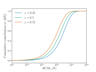
Figure 1: Cumulative contribution to the $\langle bP_{e}\rangle$ integral from theoretical estimates (using AGN feedback pressure profile described in §II.2) of Eq. 15 as a function of halo mass. Most contribution to the integral comes from halos in the range $10^{13}$ to $10^{15}$ $M_{\odot}/h$. There is significant contribution to $\langle bP_{e}\rangle$ from halos with $M<10^{14}\,M_{\odot}/h$; for current data, correlation analyses of the type considered here are the only way to probe this halo mass range.

We define the integral of $b_{g}$ over halos as the linear bias of our galaxy sample, i.e.

$$b_{g}(z)=\int_{0}^{\infty}\frac{N(M,z)}{\bar{n}(z)}\bigg{\langle}\frac{\rho}{M}\bigg{\rangle}\,b(M,z)\frac{dn}{dM}dM.$$ (14)

Eq. 13 can then be simplified further by defining:

$$\langle bP_{e}\rangle(z)\equiv(1+z)^{3}\int_{0}^{\infty}\frac{dn}{dM}b(M,z)E_{T}(M,z)dM.$$ (15)

This quantity represents the bias weighted thermal energy of all halos, and is the primary quantity of interest in this analysis. In order to estimate the $\langle bP_{e}\rangle$ from above equation, we use fitting formulae of halo mass function as described in Tinker et al. (2008) and large scale halo bias as descirbed in Tinker et al. (2010). We plot cumulative of the integrand of Eq. 15 at several redshifts in Fig. 1. The dominant contribution to $\langle bP_{e}\rangle$ comes from halos with masses in the range of about $3\times 10^{12}\lesssim M/(M_{\odot}/h)\lesssim 10^{15}$.

In the two-halo limit, the galaxy-pressure cross-power spectrum then simplifies to:

$$P^{\rm two-halo}_{Pg}(k,z)=b_{g}(z)\langle bP_{e}(z)\rangle P_{\rm lin}(k,z).$$ (16)

Substituting back into Eq. 5, the two-halo contribution to the galaxy-$y$ cross-correlation function becomes

$$\xi^{\rm two-halo}_{yg}(R,z)=\frac{\sigma_{T}}{m_{e}c^{2}}b_{g}(z)\langle bP_{e}(z)\rangle\\ \frac{1}{1+z}\int_{-\infty}^{\infty}d\chi\hskip 2.84544pt\xi_{\rm lin}\Bigg{(}\sqrt{\chi^{2}+R^{2}},z\Bigg{)}.$$ (17)

The integral in the above equation is the projected linear correlation function, $w_{p,lin}(R)$. So, succinctly, our model for the cross-correlation function becomes:

$$\xi^{\rm two-halo}_{yg}(R,z)=\frac{\sigma_{T}}{m_{e}c^{2}}b_{g}(z)\langle bP_{e}(z)\rangle\frac{w_{p,\rm{lin}}(R,z)}{1+z}.$$ (18)

A CMB experiment like Planck observes the sky convolved with a beam, which we must account for. To do this, we first transform the above equation to angular space. Since $R$ denotes the comoving size of a halo, we have $\theta=R/\chi(z)$, where $\chi(z)$ is the comoving distance to redshift $z$. In Fourier space, the halo-y cross-power spectrum is:

$$C^{\ell}_{yg}=\frac{\sigma_{T}}{m_{e}c^{2}}b_{g}(z)\langle bP_{e}\rangle\int d\theta\,2\pi\theta J_{0}(\ell\theta)\frac{w_{p,\rm{lin}}(\chi(z)\theta)}{1+z},$$ (19)

where $J_{0}$ is the Bessel function of the first kind.

Multiplying this power spectrum by the beam function, $B(\ell)$, and then inverse Fourier transforming, we obtain:

$$\xi^{s,\rm two-halo}_{yg}(\chi\theta,z)=\int\frac{d\ell\,\ell}{2\pi}J_{0}(\ell\theta)C_{yg}(\ell)B(\ell).$$ (20)

We thus obtain in the two-halo limit (see also V17):

$$\xi^{s,\rm two-halo}_{yg}(R,z)\approx\frac{\sigma_{T}}{m_{e}c^{2}}b_{g}(z)\langle bP_{e}(z)\rangle\frac{w^{S}_{\rm lin}(R,z)}{1+z},$$ (21)

where $w^{S}_{\rm lin}(R,z)$ is the projected linear correlation function, smoothed by the beam as shown above.

Eq. 21 describes the cross-correlation between galaxies and $y$ at a fixed redshift. The redMaGiC galaxies, however, are distributed over a broad redshift range, so we must average Eq. 21 over the normalized redshift distribution, $\omega^{i}(z)$, of the $i$th redMaGiC galaxy bin. Since the bias and bias-weighted pressure are expected to evolve slowly with redshift, and since the individual redshift bins of the redMaGiC galaxies are only $\Delta z\sim 0.15$, we can define effective parameters over the whole bin, $b_{g}$ and $\langle bP_{e}\rangle$. The projected correlation function is also averaged across the redshift bins in this way. Our final model for the galaxy-y cross-correlation is given by:

$$\xi^{s,i}_{yg}(R>>r_{\rm vir},\bar{z})\approx\frac{\sigma_{T}}{m_{e}c^{2}}b^{i}_{g}\langle bP_{e}\rangle^{i}\int_{0}^{\infty}\frac{w^{S}_{\rm lin}(R,z)\omega^{i}(z)}{1+z}dz.$$ (22)

Given a cosmological model, $w^{S}_{\rm lin}(R)$ is fixed. Consequently, specifying $b_{g}$ and $\langle bP_{e}\rangle$ is sufficient to specify the galaxy-$y$ cross-correlation function. As we will show below, we can determine $b_{g}$ using fits to the galaxy-galaxy correlation function, allowing us to use the galaxy-$y$ measurements to solve for $\langle bP_{e}\rangle$.

II.2 Pressure profile model

Until now, we have been agnostic about the form of the halo pressure profile, $P_{e}(r,M,z)$. Battaglia et al. (2012) (hereafter B12) measured the pressure profiles of halos in hydrodynamical simulations, and we will use fitting functions from those measurements in our analysis below. The B12 fits use spherical overdensity definitions of the halo mass and radius, $M_{\Delta}$ and $R_{\Delta}$, respectively. These are defined such that the mean density within $R_{\Delta}$ is $\Delta$ times critical density, $\rho_{\rm crit}(z)$, i.e.:

$$M_{\Delta}=\Delta\frac{4}{3}\pi R_{\Delta}^{3}\ \rho_{\rm crit}(z).$$ (23)

We will use both $\Delta=200$ and $\Delta=500$ definitions below where convenient. The B12 pressure profile fitting function is then a generalized NFW model:

$$P(x=r/R_{\Delta},M_{\Delta},z)=P_{\Delta}P_{0}(x/x_{c})^{\gamma}\left[1+(x/x_{c})^{\alpha}\right]^{-\beta},$$ (24)

where $\gamma$, $\alpha$, $\beta$ and $x_{c}$ are redshift and mass dependent parameters of the model and the pressure normalization, $P_{\Delta}$, is given by:

$$P_{\Delta}=\Delta\ \rho_{\rm crit}(z)\frac{\Omega_{b}}{\Omega_{m}}\frac{GM_{\Delta}}{2R_{\Delta}},$$ (25)

where $\Omega_{b}$ and $\Omega_{m}$ are the baryon and matter fractions, respectively, at redshift $z=0$. Because of significant degeneracy between the parameters, B12 set $\alpha=1.0$ and $\gamma=-0.3$.

The free parameters of the B12 fits are then $P_{0}$, $x_{c}$ and $\beta$. B12 additionally modelled the mass and redshift dependence of these parameters using fits of the form

$$A=A_{0}\left(\frac{M_{200}}{10^{14}M_{\odot}}\right)^{\alpha_{m}}(1+z)^{\alpha_{z}},$$ (26)

where $A$ represents $P_{0}$, $x_{c}$ or $\beta$. The best fit parameters are given in Table 1 of B12.

B12 considered different models for gas heating, described in more detail in Battaglia et al. (2010) (hereafter B10). In our analysis of the data we primarily rely on the ‘shock heating’ model from B10. In this model, gas is shock heated during infall into the cluster potential; no additional energy sources or cooling models are included. Below, we will extend this model to include the possibility of additional energy sources, which we will use the data to constrain. For the purposes of generating simulated $y$ maps, we will also employ the AGN feedback model from B10, which includes a prescription for radiative cooling, star formation, and supernovae feedback, in addition to AGN.

The quantity $\langle bP_{e}\rangle$ depends on the full pressure profile of the halos, and is therefore sensitive to its behavior at large $r$. At distances $r\gtrsim 2R_{200}$, B12 found that the pressure profile fits could depart from the mean profile in simulations by more than 5%. In our analysis, when computing $\langle bP_{e}\rangle$, we will truncate the model pressure profiles at $r=3R_{500}$. We will consider the impact of varying this choice in §V.2. Additionally, the $\langle bP_{e}\rangle$ integral receives some contribution from $M\sim 10^{13}\,M_{\odot}/h$ halos, below the halo mass limit of the B10 simulations. Consequently, when we model $\langle bP_{e}\rangle$ we will effectively be extrapolating the B10 fits to a regime just below where they were calibrated.

II.3 Model for additional energy sources

The main purpose of our analysis is to constrain the amount of energy in the halo gas relative to that expected from gravitational collapse. The energetics of the halo gas could be changed relative to the gravitational expectation by processes such as AGN feedback and cooling. As described above, the observable quantity $\langle bP_{e}\rangle$ is sensitive to the total thermal energy in halos in the mass range from about $10^{13}$ to $10^{15}\,M_{\odot}$. To constrain departures from the purely gravitational energy input to the gas, we adopt the model

$$E_{T}(M)=E_{T}^{\rm sh}(M)(1+\alpha(M)),$$ (27)

where $E_{T}^{\rm sh}(M)$ is the thermal energy computed as in Eq. 11 using the shock heating model for the pressure profile from B12 (i.e. gravitational energy input only, and no cooling). We adopt a simple phenomenological model for $\alpha(M)$:

$$\alpha(M)=\begin{cases}\alpha&\text{if\,}M<M_{\rm th}\\ 0&\text{if\,}M>M_{\rm th}\end{cases},$$ (28)

where $\alpha$ is a constant. The motivation for introducing $M_{\rm th}$ is that for very massive halos, we expect the gravitational energy to dominate over all other energy sources. Below, we will set $M_{\rm th}=10^{14}\,M_{\odot}$, although we will also consider the impact of taking $M_{\rm th}\rightarrow\infty$.

We emphasize that $\langle bP_{e}\rangle$ is sensitive to the total thermal energy in halos. Any process which changes the pressure profile, but does not change the total thermal energy content should not change $\langle bP_{e}\rangle$. Such process might include, for instance, bulk motions of gas. An additional point worth emphasizing is that the $\langle bP_{e}\rangle$ measurements for a particular redshift bin constrain the total thermal energy in the halos at that redshift. This thermal energy could be impacted by heating or cooling at higher redshift. For instance, AGN feedback at $z>1$ could impact the measured $\langle bP_{e}\rangle$, provided that gas has not had sufficient time to cool by the redshift of observation.

II.4 Model for galaxy-galaxy clustering

At fixed cosmology, Eq. 21 shows that the galaxy-$y$ cross-correlation in the two-halo regime is completely determined once $\langle bP_{e}\rangle$ and $b_{g}$ are specified. We can break the degeneracy between the two quantities using information from galaxy clustering, which is sensitive to $b_{g}$, but not $\langle bP_{e}\rangle$. By performing a joint fit to the galaxy-$y$ and galaxy-galaxy correlation functions, we can therefore constrain $\langle bP_{e}\rangle$ as a function of $z$.

To constrain $b_{g}$ we rely on measurements of galaxy-galaxy clustering. We now develop a model for this observable in the two-halo regime. The power spectrum of the galaxies in the two-halo regime is given by:

$$P^{\rm two-halo}_{gg}(k,z)=\\ \bigg{[}\int dM\frac{dn}{dM}\frac{N(M,z)}{\bar{n}(z)}u_{m}(k,M,z)b(M,z)\bigg{]}^{2}P_{\rm lin}(k,z).$$ (29)

In the two-halo regime, we can take the low-$k$ limit for the dark matter halo profile $u_{m}(k,M,z)$, yielding:

$$P^{\rm two-halo}_{gg}(k,z)=\\ \bigg{[}\int dM\frac{dn}{dM}\frac{N(M,z)}{\bar{n}(z)}\bigg{\langle}\frac{\rho}{M}\bigg{\rangle}b(M,z)\bigg{]}^{2}P_{\rm lin}(k,z).$$ (30)

Using the same definition of $b_{g}$ as in Eq. 14, we find the galaxy-galaxy power spectrum to be:

$$P^{\rm two-halo}_{gg}(k,z)=b_{g}(z)^{2}P_{\rm lin}(k,z).$$ (31)

The Limber approximation (Limber, 1953; Loverde & Afshordi, 2008) can then be used to relate the 3D power spectrum to the harmonic-space power spectrum on the sky:

$$C_{gg}(\ell)=\int d\chi\frac{q^{2}_{g}(z)}{\chi^{2}}P_{\rm lin}\left(\frac{\ell+1/2}{\chi},\chi\right),$$ (32)

where $q$ is the weight function given by:

$$q_{g}(z)=b_{g}\omega(z)\frac{dz}{d\chi}.$$ (33)

The angular correlation functions can then be related to the harmonic cross-spectra for any given redshift bin i via:

$$w^{ii}(\theta)=\sum_{\ell}\frac{2\ell+1}{4\pi}P_{\ell}\left(\cos(\theta)\right)\,C_{gg}^{ii}(\ell)\,$$ (34)

where $P_{\ell}\left(\cos(\theta)\right)$ is the Legendre polynomial of the $\ell$-th order. We note that this model is equivalent to that employed in the DES Collaboration et al. (2017) analysis, which uses the same galaxy clustering measurements as employed here.

III Data

III.1 DES redMaGiC catalog

The primary goal of this analysis is to constrain the redshift evolution of the pressure of the Universe by measuring the correlation between galaxies and maps of the Compton-$y$ parameter. To this end, we require a sample of galaxies that have well measured redshifts, and which can be detected out to large redshift. An ideal catalog for this purpose is the redMaGiC catalog (DES Collaboration et al., 2017) derived from first year (Y1) DES observations.

The Dark Energy Survey is a 5.5 year survey of 5000 sq. deg. of the southern sky in five optical bands (g, r, i, z, and $Y$) to a depth of $r>24$. In this analysis, we use first Y1 data from DES covering approximately 1321 sq. deg. to roughly $r\sim 23$ (Flaugher et al., 2015; Dark Energy Survey Collaboration et al., 2016).

redMaGiC galaxies are identified in DES data based on a fit to a red sequence template using the methods described in Rozo et al. (2016). The photometric accuracy of the selection is high: $\sigma_{\rm rmg}=0.0167(1+z)$. For details of the validation of the redMaGiC redshift estimates, see Rozo et al. (2016) and Cawthon et al. (2018).

Throughout this analysis, we use the same selection of galaxies and redshift binning as used in the analysis of DES Collaboration et al. (2017). Using the same selection as in DES Collaboration et al. (2017) is advantageous since systematic errors in the redshift estimates for this sample have been thoroughly studied in Cawthon et al. (2018), and the impact of observational systematics on redMaGiC galaxy detection have been studied in Elvin-Poole et al. (2018).

The Y1 redMaGiC sample was divided into five redshift bins from $z=0.15$ to $z=0.9$. The first three redshift bins use a luminosity cut of $L/L_{*}>0.5$, while the fourth and fifth redshift bins use cuts of $L/L_{*}>1.0$ and $L/L_{*}>1.5$, respectively, where $L_{*}$ is computed using a Bruzual and Charlot model (Bruzual & Charlot, 2003), as described in Rozo et al. (2016). Given the small number of galaxies in the fifth bin and the potential for higher contamination of the galaxy-$y$ cross-correlation measurements in that bin (see below), we restrict our analysis to the first four redshift bins.

Galaxies are placed into redshift bins based on their photometric redshift as estimated by the redMaGiC algorithm Rozo et al. (2016). redMaGiC assigns a redshift estimate, $z_{\rm rmg}$, to each galaxy. The estimated $\omega(z)$ for each bin is then computed as a sum of Gaussian probability distribution functions centered at $z^{i}_{\rm rmg}$, with standard deviation $\sigma_{\rm rmg}$. The corresponding redshift distributions are shown in Fig. 2.

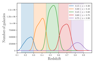
Figure 2: Redshift distributions of Y1 redMaGiC galaxies used in this analysis. The galaxy sample is divided into five redshift bins, which are identical to the ones used in DES Collaboration et al. (2017). We only use the first four of these bins in the present analysis, as described in §III.1. The integral of each curve over $dz$ is equal to the number of galaxies in the bin. In total, the sample contains approximately 600,000 galaxies.

III.2 Planck maps

We correlate the redMaGiC galaxies with maps of the Compton-$y$ parameter derived from Planck data. Planck observed the sky in nine frequency bands from 30 GHz to 857 GHz from 2009 to 2013 (Tauber et al., 2010; Planck Collaboration et al., 2011a). The resolution of the Planck experiment is band dependent, varying from roughly 30 arcminutes at the lowest frequencies to 5 arcminutes at the highest.

We use the publicly available 2015 Planck High Frequency Instrument (HFI) and Low Frequency Instrument (LFI) maps in this analysis (Planck Collaboration et al., 2016a, b) and construct Compton-$y$ maps using the Needlet Internal Linear Combination (NILC) algorithm that is described in Delabrouille et al. (2009) and Guilloux et al. (2007). For comparison, we will also make use of the publicly available Planck estimates of $y$ described in Aghanim et al. (2015) which uses the same set of temperature maps.

While constructing various versions of Compton-$y$ map (see below), we use the same galactic mask as used in Aghanim et al. (2015) which blocks 2% of the sky area (mostly in the galactic center). We also use the point source mask which is the union of the individual frequency point-source masks discussed in Planck Collaboration et al. (2014b).

III.3 Simulated sky maps

One of the primary concerns for the present analysis is possible contamination of the estimated $y$ maps by astrophysical foregrounds. The most significant potential contaminant is the cosmic infrared background (CIB), which is predominantly sourced by thermal emission from galaxies throughout the Universe. CIB emission comes from a broad range of redshifts, roughly $z\sim 0.1$ to 4.0, with the bulk of emission coming from $z\gtrsim 1$ (e.g. Schmidt et al., 2015). The majority of CIB emission is therefore beyond the redshift range of the galaxies considered in this analysis, and will therefore be uncorrelated with the redMaGiC galaxies. Such emission could constitute an additional noise source, but will not in general lead to a bias in the estimated galaxy-$y$ cross-correlation functions.

However, some CIB emission is sourced from $z\lesssim 0.7$, which overlaps with the redshift range of the redMaGiC galaxies. Since the CIB is traces the large-scale structure, it will be correlated with the redMaGiC galaxies. Consequently, any leakage of CIB into the estimated $y$ maps over this redshift range could result in a bias to the estimated galaxy-$y$ cross-correlation functions.

Another possible source of contamination is bright radio sources. Although the brightest sources are detected and masked, there will also be radio point sources that are not individually detected. For instance, in a recent study by Shirasaki (2019), it was found that radio sources can bias the tSZ-lensing correlation when using Planck data. Lastly, we may also have to worry about the potential biases and loss of signal-to-noise that may arise due to galactic dust contamination. We assess the effects of all the above mentioned biases using simulated sky maps as described below.

We rely on both the Websky mocks and the Sehgal et al. (2010) simulations. These two sets of simulations are useful in this analysis because they have produced correlated CIB maps and partially cover the frequency range used by Planck.

The Websky mocks are full sky simulations of the extragalactic microwave sky generated using the mass-Peak Patch approach, which is a fully predictive initial-space algorithm, and a fast alternative to a full N-body simulation. As described in Stein et al. (2018), the mass-Peak Patch method finds an overcomplete set of just-collapsed structures through coarse-grained ellipsoidal dynamics and then resolves those structures further. These maps are provided for frequencies 143, 217, 353, 545, and 857 GHz which are very similar to the Planck HFI channels.

The Sehgal et al. (2010) simulations are another set of full sky simulations which provide maps for the cosmic microwave background, tSZ, kinetic SZ, populations of dusty star forming galaxies, populations of galaxies that emit strongly at radio wavelengths, and dust from the Milky Way galaxy. Maps are provided at six different frequencies: 30, 90, 148, 219, 277, and 350 GHz which are very similar to the Planck LFI channels and some of the HFI channels. These sets of maps allow us to directly test the effects of bright radio sources and galactic dust on the Compton-$y$ and its cross-correlation with halos that populate redMaGiC -like galaxies.

We generate simulated sky maps in Healpixformat by combining the various component maps from the simulations described above. For the Websky mocks, we combine Compton-$y$, lensed CMB and CIB; for the Sehgal simulations, we combine Compton-$y$, lensed CMB, CIB, radio galaxies and Milky Way galactic dust emission. The "true" sky maps are then convolved with Gaussian beams with frequency-dependent full width half maxima (FWHM) corresponding to the Planck data. Finally, we add Planck-like white noise to each channel at the levels given in Table 6 of Planck Collaboration et al. (2014a).

III.4 MICE and Buzzard N-body simulations

In addition to the estimation of $y$ from the Planck maps, the other major step in our analysis is the inference of $\langle bP_{e}\rangle$ from the measured correlation functions. In order to test the methodology and assumptions involved in this step of the analysis, we rely on simulated redMaGiC galaxy catalogs and $y$ maps. The simulations used for this purpose are the MICE (Fosalba et al., 2015b; Carretero et al., 2015; Fosalba et al., 2015a) and Buzzard (DeRose et al., 2019) N-body simulations. Both simulations have been populated with galaxy samples approximating redMaGiC .

MICE Grand Challenge simulation (MICE-GC) is an N-body simulation run on a 3 Gpc/$h$ box with $4096^{3}$ particles produced using the Gadget-2 code (Springel, 2005). The mass resolution of this simulation is $2.93\times 10^{10}M_{\odot}/h$ across the full redshift range that we analyze here ($z<0.75$), and halos are identified using a FoF algorithm using a linking length of 0.2. These halos are then populated with galaxies using a hybrid sub-halo abundance matching and a halo occupation distribution (HOD) approach, as detailed in Carretero et al. (2015). These methods are designed to match the joint distributions of luminosity, $g-r$ color, and clustering amplitude observed in SDSS (Zehavi et al., 2005). The construction of the halo and galaxy catalogs is described in Crocce et al. (2015). A DES Y1-like catalog of galaxies with the spatial depth variations matching the real DES Y1 data is generated as described in MacCrann et al. (2018). MICE assumes a flat $\Lambda$CDM cosmological model with $h=0.7$, $\Omega_{\rm m}=0.25$, $\Omega_{b}=0.044$ and $\sigma_{8}=0.8$.

Buzzard is a suite of simulated DES Y1-like galaxy catalogs constructed from dark matter-only N-body lightcones and including galaxies with DES $griz$ magnitudes with photometric errors, shape noise, and redshift uncertainties appropriate for the DES Y1 data (DeRose et al., 2019). This simulation is run using the code L-Gadget2 which is a proprietary version of the Gadget-2 code and the galaxy catalogs are built from the lightcone simulations using the ADDGALS algorithm (DeRose et al., 2019; MacCrann et al., 2018; Weschler, R. et al., prep). Spherical-overdensity masses are assigned to all halos in Buzzard . Buzzard assumes a flat $\Lambda$CDM cosmological model with $h=0.7$, $\Omega_{\rm m}=0.286$, $\Omega_{b}=0.047$ and $\sigma_{8}=0.82$.

We generate mock Compton-$y$ maps for the N-body simulations by pasting $y$ profiles into mock sky maps at the locations of simulated halos. The $y$ profile used for this purpose is the AGN feedback model (with $\Delta=200$) from Table 1 of B12. This approach to generating Compton-$y$ maps misses contributions to $y$ from halos below the resolution limit of the simulation. However, given that Buzzard and MICE identify halos above $3\times 10^{12}M_{\odot}/h$ and $10^{11}M_{\odot}/h$, respectively, Fig. 1 shows that for both simulations, we capture at least 95% of the contribution to $\langle bP_{e}\rangle$. Since the statistical errors on the simulation measurements are significantly larger than $5\%$, any missing contribution to $\langle bP_{e}\rangle$ is not important for this work. Note that since MICE uses only FoF masses, it is not strictly correct to apply the B12 profile to these halo mass estimates. However, this inconsistency should not impact our validation tests described below.

IV Analysis

IV.1 Measuring the galaxy-$y$ cross-correlation and galaxy-galaxy clustering

Our estimator for the galaxy-$y$ cross-correlation for galaxies in a single redshift bin and in the angular bin labeled by $\theta_{\alpha}$ is

$$\hat{\xi}^{yg}(\theta_{\alpha})=\frac{1}{N_{D}}\sum^{N_{D}}_{ij}y_{m}f(\theta_{ij})-\frac{1}{N_{R}}\sum_{i_{R}j}^{N_{R}}y_{m}f(\theta_{i_{R}j}),$$ (35)

where $i$ ($i_{R}$) labels a galaxy (random point), $m$ labels a map pixel, $\theta_{im}$ is the angle between point $i$ and map pixel $m$, and $f$ is an indicator function such that $f(\theta)=1$ if $\theta$ is in the bin $\theta_{\alpha}$ and $f(\theta)=0$ otherwise. The total number of galaxies and random points are $N_{D}$ and $N_{R}$, respectively. By subtracting the cross-correlation of random points with $y$, we can undo the effects of chance correlations between the mask and the underlying $y$ field.

We measure the galaxy-galaxy correlation using the standard Landy & Szalay (1993) estimator. Because we use the same catalogs, redshift bins, and angular bins as in Elvin-Poole et al. (2018), our measurements of clustering of the redMaGiC galaxies are identical to those in Elvin-Poole et al. (2018). For both the galaxy-$y$ and galaxy-galaxy correlations, we compute the estimators using TreeCorr (Jarvis et al., 2004).

We measure the galaxy-$y$ cross-correlation in 20 radial bins from 1 Mpc/$h$ to 40 Mpc/$h$. We measure galaxy-galaxy clustering in 20 angular bins from 2.5 arcmin to 250 arcmin which is the binning used in Elvin-Poole et al. (2018). However, as described below in §IV.5, we do not include all measured scales when fitting these correlation functions, since the model is not expected to be valid at all scales. Our angular scale cut choices are validated in §IV.6.

IV.2 Covariance Estimation

Jointly fitting the measurements of the galaxy-$y$ and galaxy-galaxy correlations requires an estimate of the joint covariance between these two observables. For this purpose, we use a hybrid covariance matrix estimate built from a combination of jackknife and theoretical estimates. We validate the covariance estimation in §IV.6.

For the covariance block describing only the galaxy clustering measurements, we use the theoretical halo-model based covariance described in Krause et al. (2017). This covariance has been extensively validated as part of the DES Collaboration et al. (2017) analysis.

For the block describing the galaxy-$y$ covariance and for the cross-term blocks between galaxy-$y$ and galaxy clustering, we use jackknife estimates of the covariance. The use of a jackknife is well motivated because several noise sources in the $\hat{y}$ map are difficult to estimate. These include noise from CIB and galactic dust. Since the jackknife method uses the data itself to determine the covariance, it naturally captures these noise sources.

The jackknife method for estimating the covariance of correlation functions on the sky is described in Norberg et al. (2009). To construct jackknife patches on the sky, we use the KMeans algorithm. We find that 800 jackknife patches is sufficient for robust covariance estimation. This means that each jackknife patch is approximately 85 arcmin across, which is approximately 1.5 times larger than our maximum measured scale for each redshift bin.

Our jackknife estimates of the cross-covariance between the galaxy-clustering and galaxy-$y$ measurements are noisy. When applying the jackknife covariance estimation to simulations (see §IV.6), we find that this cross-covariance is largest when it is between two of the same redshift bins, as expected. For the simulated measurements, zeroing cross-covariance between clustering and galaxy-$y$ measurements of different redshift bins has no impact on the inferred $\langle bP_{e}\rangle$. To reduce the impact of noise in our covariance estimates, we therefore set these blocks to zero in our data estimate of the covariance. The final covariance estimate is shown in Fig. 11.

IV.3 $y$ map estimation

IV.4 Overview

The $y$ signal on the sky can be estimated as a linear combination of multi-frequency maps. The constrained internal linear combination (CILC) method chooses weights in the linear combination that:

• (a) impose the constraint that the estimator has unit response to a component with the frequency dependence of $y$,

• (b) impose a constraint that the estimator has null response to some other component with known frequency dependence,

• (c) minimize the variance of the estimator subject to the constraints from (a) and (b). Below, we will consider several different analysis variations that attempt to null different components (or none at all).

Note that the more components that are "nulled," the larger the variance of the resultant estimator, since imposing the nulling condition effectively reduces the number of degrees of freedom that can be used to minimize the variance.

When forming the estimated $y$ map with the CILC, the multi-frequency maps themselves must be decomposed into some set of basis functions, such as pixels or spherical harmonics. In this analysis, we use maps decomposed using the needlet frame on the sphere (Guilloux et al., 2007; Marinucci et al., 2008; Delabrouille et al., 2009). The Planck estimate of $y$ generated using CILC methods in the needlet frame goes under the name Needlet Internal Linear Combination (NILC) and is described in Aghanim et al. (2015). We will use both the Planck NILC map and also construct our own versions for the purposes of testing biases due to contamination by the CIB and other astrophysical foregrounds. A brief description of the analysis choices and methodology is given in §IV.4.1; details are provided in Appendix A.

IV.4.1 Attempting to mitigate CIB bias in the $y$ map

The Planck NILC $\hat{y}$ map (Aghanim et al., 2015) enforces null response to components on the sky with the same frequency dependence as the CMB. This choice is well motivated, since the CMB constitutes the dominant noise source over the frequency range that has significant signal-to-noise for the estimation of $y$. We will refer to this choice as unit-y-null-cmb. We will also consider a variation that does not explicitly null any components, which we refer to as unit-y.

In the end, however, we only care about the cross-correlation of $\hat{y}$ with galaxies. The CMB correlates only very minimally with galaxies (due, for instance, to the integrated Sachs-Wolfe effect), and so should not result in a bias to the estimated galaxy-$y$ cross-correlation functions. Since the CILC imposes a minimum variance condition on $\hat{y}$, explicitly nulling the CMB is not necessary for our purposes. Attempting to null the CIB, on the other hand, is well motivated to prevent potential biases in the $\langle bP_{e}\rangle$ estimation; we call this method unit-y-null-cib. To null the CIB, one must adopt some reasonable choice for its frequency dependence. Unfortunately, the frequency dependence of the CIB signal is uncertain, and furthermore, may vary with redshift, angular scale, or position on the sky.

We determine the frequency scaling of the CIB in the Sehgal simulations and the Websky mocks by cross-correlating the mock halos with the mock CIB maps. To approximate the redMaGiC selection, we correlate halos in the mass range $2\times 10^{13}M_{\odot}/h<M<3\times 10^{13}M_{\odot}/h$ and redshift range $0.45<z<0.6$ with the simulated CIB maps. We then measure the frequency scaling of these correlations at 100 arcmin, near the regime of interest for our $\langle bP_{e}\rangle$ constraints. We compare this fiducial CIB frequency dependence to Planck (Planck Collaboration et al., 2011b) and Sehgal simulations in Fig. 3. The Planck points are derived from the rms fluctuations of the CIB anisotropy spectrum over the range $200<\ell<2000$. We note these measurements are consistent with the frequency scaling of the mean of the CIB field, as described in Planck Collaboration et al. (2011b).

Fig. 3 shows that the frequency dependence of the CIB in both the simulations and the Planck data are consistent at roughly the 10% level over the frequency range relevant to this analysis. Larger deviations are observed at 545 and 857 GHz, but these channels are not used in the $y$ map reconstruction (see below). We also show the redshift dependence of the frequency scaling by cross-correlating with halos in different redshift bins, finding some variation. As mass of halos hosting the redMaGiC galaxies is not completely certain, we also test the dependence of the CIB frequency scaling on the mass of halo used for cross-correlation.

The CIB intensity rises quickly at the higher frequency channels of Planck. In order to reduce potential CIB contamination of the $y$ maps, we do not use the 545 or 857 GHz channels in our $y$ map reconstruction. This choice differs from that made by Aghanim et al. (2015), where both the 545 and 857 GHz channels were employed. We see that variations in halo selection criteria impact the frequency dependence of CIB by less than 20% for frequency channels below 545 GHz. We have found that this choice makes the reconstructed $y$ maps less sensitive to the details of the CIB modelling, with only a minor degradation in signal-to-noise.

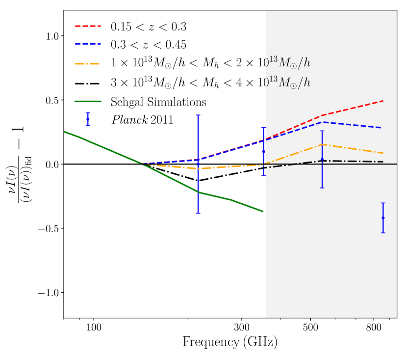
Figure 3: Frequency scaling of the halo-CIB correlation in the Websky mocks for different halo selections in redshift (dashed) and mass (dot-dashed). Measurements are shown relative to the fiducial CIB model, as described in the text. We also show the frequency scaling of the CIB in the Sehgal simulations (green solid curve), and the measurements from Planck Collaboration et al. (2011a) (blue points with errorbars). For frequencies less than 545 GHz (i.e. the frequency range used in this analysis, corresponding to the unshaded region in this plot), departures from our fiducial CIB model are less than 20%, and are consistent with the Planck measurements.

Finally, when analyzing the Sehgal mocks, we employ a large scale contiguous apodized mask that covers 10% of the sky (near the galactic plane) in all the temperature maps to minimize the biases that might result from bright pixels in galactic plane. To minimize similar issues due to bright radio sources, we apply a point source mask that covers radio galaxies in the top decile. This mask is similar to the point source mask provided by the Planck collaboration that we use in the analysis of data. Since this is a highly non-contiguous mask, we inpaint masked pixels in the temperature maps.

IV.4.2 Validation of $y$ estimation with mock skys

We apply our NILC pipeline to the simulated skies described in §III.3, making the three nulling condition choices described above. We correlate the resultant $y$ maps with a sample of halos that approximate the redMaGiC selection, with $2\times 10^{13}M_{\odot}/h<M_{h}<3\times 10^{13}M_{\odot}/h$. The correlation results for the Sehgal simulation with halos in the redshift range $0.15<z<0.3$ are shown in Fig. 4. In general, all three methods yield roughly consistent results that are also in good agreement with the true correlation signal.

The CIB model of the Sehgal simulations is not complete in the sense that it does not capture CIB contributions from halos below the mass limit of the simulation. The CIB frequency model assumed in the Sehgal simulations is also somewhat out of date, and does not match current Planck observations. For these reasons, we additionally use the Websky mocks for testing potential CIB biases. The Websky mocks employ a model for CIB contributions from halos below the mass limit of the simulation, and also shows better agreement with recent Planck constraints on the CIB frequency dependence. However, because the Websky mocks do not include radio sources or galactic dust, we primarily rely on the Sehgal simulations for validation. We discuss tests using the Websky mocks in §B.

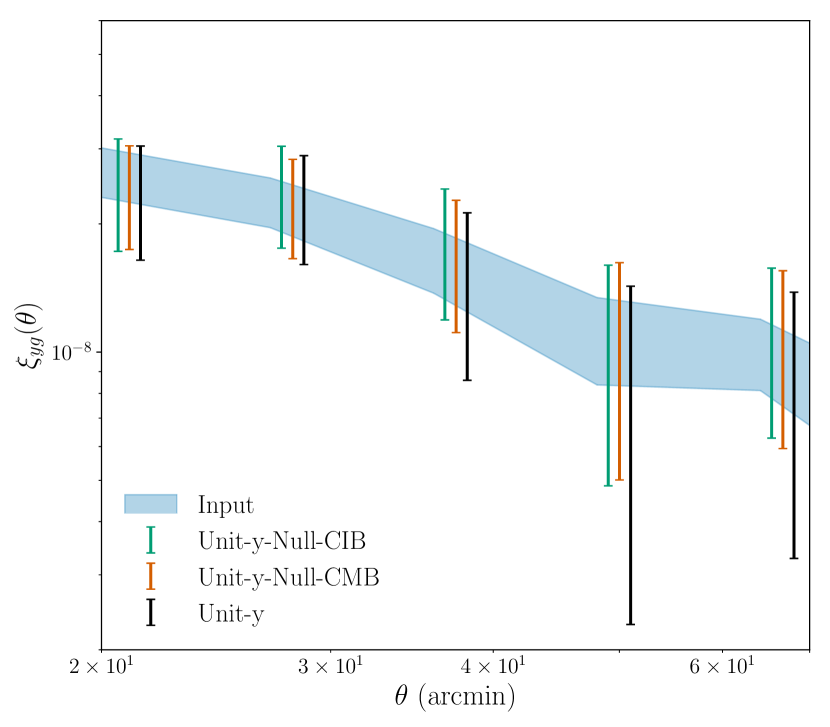
Figure 4: Galaxy-$y$ cross-correlation measurements with reconstructed $y$ maps from the Sehgal simulations. We show results for the halo bin with $2\times 10^{13}M_{\odot}/h<M_{h}<3\times 10^{13}M_{\odot}/h$ and $0.15<z<0.3$. The results for other redshift bins are similar. We find that our $y$ reconstruction methods are sufficient to recover an essentially unbiased estimate of the halo-$y$ cross-correlation over the scales of interest.

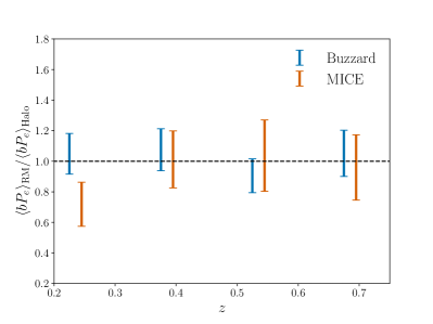
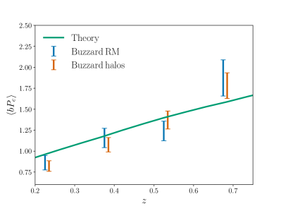
Figure 5: Left panel shows the ratio of $\langle bP_{e}\rangle$ inferred in simulations from measurements with redMaGiC galaxies to that inferred from halos. For both the Buzzard (blue) and MICE (orange) simulations, the redMaGiC galaxies and halos lead to consistent determinations of $\langle bP_{e}\rangle$. This supports the notion that the measurements are sufficiently far in the two-halo regime that the inference of $\langle bP_{e}\rangle$ is independent of the halo-galaxy connection. Right panel shows the measurements of $\langle bP_{e}\rangle$ in the Buzzard simulation compared to the theoretical prediction.

IV.5 Model fitting

Our measurements of the galaxy-$y$ and galaxy-galaxy correlations in different redshift bins can be concatenated to form a single data vector

$$\vec{d}=\left(d^{gg}_{1},d^{gy}_{1},d^{gg}_{2},d^{gy}_{2},\ldots,d^{gg}_{4},d^{gy}_{4}\right),$$ (36)

where $d^{gg}_{i}$ and $d^{gy}_{i}$ are the clustering and galaxy-$y$ correlations measurements in the $i$th redshift bin, respectively. We consider a Gaussian likelihood for the data:

$$\mathcal{L}(\vec{d}\ |\ \vec{\theta})=-\frac{1}{2}\left(\vec{d}-\vec{m}(\vec{\theta})\right)^{T}\mathbf{C}^{-1}\left(\vec{d}-\vec{m}(\vec{\theta})\right),$$ (37)

where $\mathbf{C}$ is the covariance matrix described in §IV.2, $\vec{\theta}$ represents the model parameters (galaxy bias, $b_{i}$, and bias-weighted pressure, $\langle bP_{e}\rangle_{i}$ for redshift bin $i$) for all redshift bins, and $\vec{m}$ represent the model vector calculated as described in §II. We adopt flat priors on all of the parameters, and sample the posterior using Monte Carlo Markov Chain methods as implemented in the code emcee (Foreman-Mackey et al., 2013).

We restrict our fits to the galaxy-galaxy correlation functions to scales $R>8\,{\rm Mpc}/h$. This restriction is imposed to ensure that the measurements are in the two-halo dominated regime, as discussed in §II, and is consistent with the scale cut choices motivated in Krause et al. (2017) and MacCrann et al. (2018).

The determination of appropriate scale cuts for the galaxy-$y$ cross-correlation is somewhat more involved. As described in Appendix IV.3, the Compton-$y$ map used in this analysis is smoothed with a beam of FWHM of $10$ arcmin. The beam has the effect of pushing power from small to large scales, and therefore shifts the location of the one-to-two-halo transition. For the highest redshift redMaGiC bins, this shift can be significant and hence we have to increase our scale cuts as we go to higher redshift bins. For the bins detailed in §III.1, we ensure that we only include the scale cuts that are approximately twice the beam size away for any given redshift bin in our analysis. This results in minimum scale cuts for each of the four redshift bins at 4, 6, 8 and 10 Mpc/$h$. For the maximum scale cut, we make sure that for each redshift bin, the size of an individual jackknife patch is approximately 1.5 times the maximum scale cut for that particular bin. To obtain a sufficiently low-noise estimate of the covariance matrix from the jackknifing procedure, we need of order 800 jackknife patches. These considerations yield maximum scale cuts for each of the 4 bins of 11, 17, 25 and 30 Mpc/$h$.

IV.6 Validation of model assumptions and pipeline

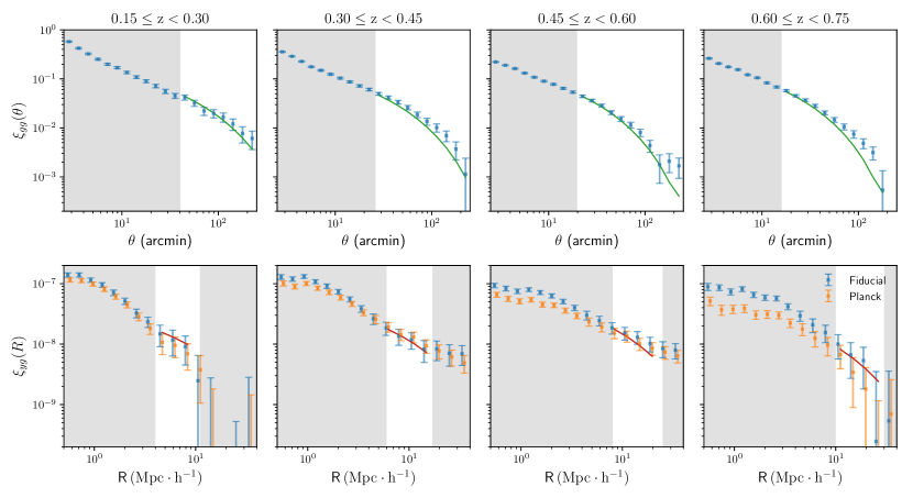
Figure 6: Measurements of the galaxy auto-correlation (top row) and Compton-y galaxy cross-correlation (bottom row) at different redshift bins corresponding to four redshift bins used in the analysis. Solid line is the best-fit to the fiducial model of Compton-$y$ which is generated after removing 545GHz and 857GHz frequency channels from the analysis. Only data in the unshaded regions are used for fitting. These scale cut choices are validated in §IV.6

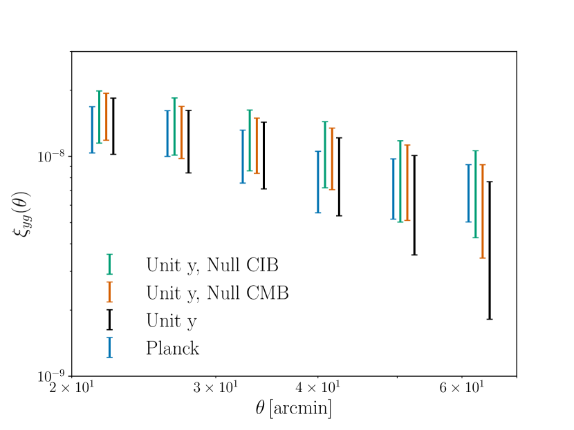
Figure 7: The galaxy-$y$ cross-correlation function over the scales of interest when the component separation method used to estimate $y$ is varied. We show the correlation measurements for the highest signal to noise redshift bin, $0.45<z<0.6$, but results for the other redshift bins are similar. We find that the estimated correlation function does not vary significantly when the $y$ estimation choices are varied. Together with our validation with simulations, this constitutes strong evidence that our correlation measurements are not significantly biased by astrophysical contaminants in the estimated $y$.

We apply our analysis pipeline to the simulated data by correlating the mock $y$ maps with both the simulated redMaGiC and halo catalogs. In the two-halo regime, both the redMaGiC galaxies and the halos should lead to consistent estimates of $\langle bP_{e}\rangle$. The left panel of Fig. 5 shows the ratio of these two measurements for both the Buzzard and MICE simulations. Indeed, we find that the redMaGiC and halo measurements are consistent in both simulations, a strong test of our modeling assumptions and methodology.

We can also compare the recovered values of $\langle bP_{e}\rangle$ from the simulations to the value computed from the Eq. 15. Since we know the true cosmological and profile parameters used to generate the simulated $y$ map, the measurement in simulations should match the theory calculation, provided our assumptions and methodology are correct. The right panel of Fig. 5 shows this comparison (using both halos and redMaGiC galaxies) for the Buzzard simulation. We find that the inferred values of $\langle bP_{e}\rangle$ are consistent with the theoretical expectation, providing a validation of our modeling, methodology, and scale cut choices. Note that we do not perform this test with the MICE simulation, since as discussed in §III.4, MICE uses FoF halo masses, while the B12 profile used to generate the simulated $y$ maps requires spherical overdensity masses.

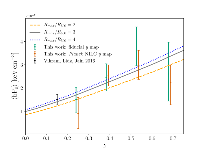
Figure 8: Constraints on the redshift evolution of the bias weighted pressure of the Universe (Eq. 15). We compare the datapoints obtained from this work with V17 and theory curves corresponding to shock heating model as described in B12. For theory curves, all models are evaluated for $\Delta=500$ and for various choices of $R_{max}/R_{\Delta}$.

.

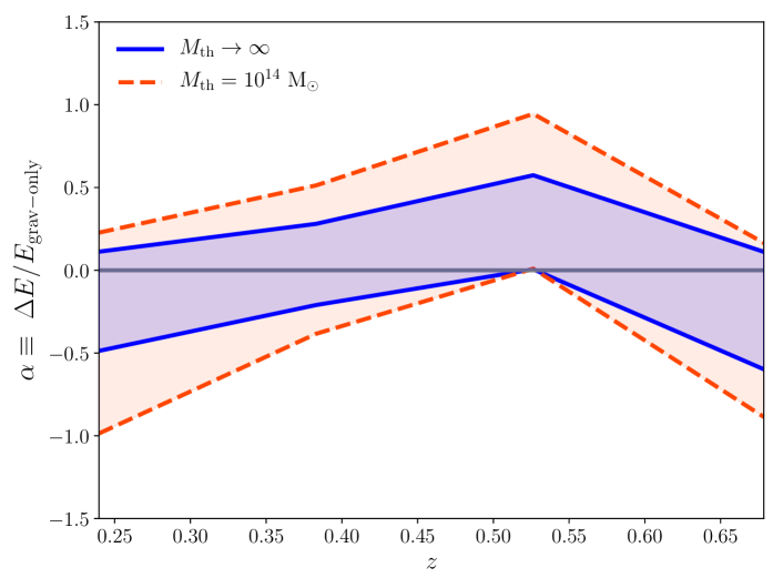
Figure 9: Constraints on the thermal energy of the gas as a function of redshift. The parameter, $\alpha$, defined in Eq. 28, measures the fractional departure of the gas thermal energy from the predictions of a model that only includes gravitational energy. Large $\alpha$ means that some process must have contributed extra thermal energy to the gas, while negative $\alpha$ means that the gas must have cooled. In our model, the addition (or deficit of) thermal energy impacts all halos below a threshold mass, $M_{\rm th}$. We show the results for $M_{\rm th}\rightarrow\infty$ (region between blue solid curves) and for $M_{\rm th}=10^{14}\,M_{\odot}$ (region between orange-red dashed curves). The $\langle bP_{e}\rangle$ measurements presented in this work are sensitive to halos with $10^{13}\lesssim M\lesssim 10^{15}\,M_{\odot}$, as shown in Fig. 1.

V Results

V.1 Galaxy-$y$ cross-correlation measurements

Our measurements of galaxy clustering (top) and the galaxy-$y$ correlation (bottom) using DES and Planck data are shown in Fig. 6. We show the galaxy-$y$ measurements with both our fiducial $\hat{y}$ map and the Planck $y$ map in Fig. 6. We obtain significant detections of galaxy-$y$ cross-correlation in all four redshift bins. Across all radial scales, the galaxy-$y$ cross-correlation is detected at a significance of $12.3$, $12.9$, $12.2$ and $8.4\sigma$ for four redshift bins in order of increasing redshift. We restrict our model fits to the scales outside of the shaded regions to ensure that we remain in the two-halo regime where our modeling approximations are valid, as discussed in §IV. The restrictions at large scales ensure that our jackknife estimate of the covariance is accurate; this cut leads to only a small degradation in signal-to-noise.

In order to assess potential biases in our measurements of the galaxy-$y$ cross-correlation, we repeat these measurements using the unit-y-null-cib and unit-y variations. In the absence of a correlated contaminant in the estimated $y$ maps, different variations on the fiducial component separation choices should not lead to significant changes in the recovered mean galaxy-$y$ cross-correlation. On the other hand, significant changes in the measured cross-correlation functions for varying component separation choices would be indicative of potential biases. Note, though, that different component separation choices can lead to significant changes in the uncertainties on the estimates of the galaxy-$y$ cross-correlation, even in the absence of any contaminant.

The impact of changing the component separation choices on the galaxy-$y$ cross-correlation measurements is shown in Fig. 7. The results are shown only for the third redshift bin of redMaGiC galaxies, since this has highest signal-to-noise. The results obtained for the other redshift bins are similar. We find that the different $y$ estimation procedures yield statistically consistent measurements of the galaxy-$y$ cross-correlation over the range of scales used in this analysis. These measurements are also consistent with the cross-correlations performed with the Planck $y$ map over the same range. The insensitivity of the galaxy-$y$ cross-correlations to the component separation choices suggests that are our measurements are not biased by astrophysical contaminants.

However, as seen in Fig. 6, there is a trend with increasing redshift for the Planck measurements at small scales to be lower in amplitude than the measurements with our fiducial $y$ map. The main difference between our fiducial $y$ map and the Planck map is that we do not use the 545 and 857 GHz channels in our $y$ reconstruction, as described in §IV.4.1. It is difficult to determine precisely the cause of the small scale discrepancy between the two $y$ map estimates seen in Fig. 6. It appears broadly consistent with contamination due to CIB, which would be expected to increase at higher redshift. We note that Aghanim et al. (2015) also found evidence for CIB bias in the tSZ angular power spectrum at small scales. We note, however, that the amount and direction of this CIB bias in the $y$ map obtained from NILC pipeline is sensitive to the frequency channels used, and that we consider here bias in galaxy-$y$ cross-correlation rather than the $y$ angular power spectrum considered in Aghanim et al. (2015). We emphasize, though, that over the range of scales fitted in this analysis, the estimates of the galaxy-$y$ correlations are consistent between the different $y$ maps.

V.2 Constraints on bias-weighted pressure

The quantity $\langle bP_{e}\rangle$, defined in Eq. 15 represents the halo bias weighted thermal energy of the gas at redshift $z$. Fig. 8 shows our constraints on this quantity as a function of redshift for two different $y$ maps: our fiducial unit-y-null-cmb map and the Planck NILC $y$ map. The measurements with the two $y$ maps appear consistent, although precisely assessing the statistical consistency is complicated by the fact that the maps are highly correlated. We find significant detections of $\langle bP_{e}\rangle$ in all redshift bins considered. The multidimensional constraints on the model parameters are shown in Fig. 12.

The black point in Fig. 8 shows the constraint on $\langle bP_{e}\rangle$ from the analysis of V17 using data from SDSS and Planck. The V17 point is at significantly lower redshift than the samples considered here ($z\sim 0.15$ as opposed to $0.2\lesssim z\lesssim 0.75$). The small errorbars on the V17 measurements result from the large area of SDSS, roughly 10,000 sq. deg. Our analysis with DES Y1 data uses roughly 1300 sq. deg, although the galaxy density of the DES Y1 measurements is significantly higher than the group catalog considered by V17.

V.3 Constraints on feedback models

The quantity $\langle bP_{e}\rangle$ depends on the cosmological parameters and on the pressure profiles of gas in halos. Given the current uncertainty on the cosmological parameters from e.g. Planck Collaboration et al. (2018), and the large model uncertainties on the gas profiles (especially at large radii), we focus on how $\langle bP_{e}\rangle$ can be used to constrain gas physics in this analysis. Fig. 1 shows that $\langle bP_{e}\rangle$ is sensitive primarily to halos with masses between $10^{13}$ and $10^{15}\,M_{\odot}$, with sensitivity to lower mass halos at high redshift. Because $\langle bP_{e}\rangle$ effectively measures the total thermal energy in halos, it is particularly sensitive to the thermodynamics of gas in halo outskirts, where the volume is large. As seen in B10, it is precisely the large-radius, high-redshift regime probed in this analysis for which the predictions of different feedback models are significantly different.

The curves in Fig. 8 show several predictions for the redshift evolution of $\langle bP_{e}\rangle$ for the ‘shock heating’ model of B12 and B10. In this model, the baryons are shock heated during infall into the cluster potential, and subsequently thermalize (with no AGN feedback or radiative cooling).

We show several model predictions in Fig. 8, corresponding to different maximum radii for the halo gas profile. In our fiducial analysis, we compute $\langle bP_{e}\rangle$ by integrating the pressure profile to $3R_{500}$. Similarly, the curve with $R_{\rm max}/R_{500}=a$ corresponds to integrating the profile to $aR_{500}$. The data is consistent with shock heating models for $a=2$, $a=3$ and $a=4$ with $\chi^{2}/\rm d.o.f.$ of $2.9/4$, $2.11/4$ and $2.26/4$, respectively.

For our fiducial shock heating model with $R_{\rm max}=3R_{500}$, we find $\chi^{2}$ per degree of freedom ($\rm d.o.f.$), $\chi^{2}/\rm d.o.f.=2.11/4$ for the cross-correlation measurements with the unit-y-null-cmb map, and $\chi^{2}/\nu=3.99/4$ for the cross-correlation with the Planck map. In both cases, the data are statistically consistent with the shock heating model from B12.

As described in §II.3, the quantity $\langle bP_{e}\rangle$ is sensitive to the (bias weighted) total thermal energy in the halo gas. We can use the measured $\langle P_{e}\rangle$ to constrain any sources of energy beyond that associated with gravitational collapse, such as could be generated by feedback. The additional energy model is described in §II.3, and parameterizes any additional energy contributions for halos with mass $M<M_{\rm th}$ as a fractional excess, $\alpha(M)$, beyond that predicted by the shock heating model from B10, which only includes gravitational energy.

The constraints on $\alpha(z)$ are shown in Fig. 9. In the limit that the threshold mass is very large ($M_{\rm th}\rightarrow\infty$, blue solid curve), we find that any mechanisms that change the thermal energy of the gas must not increase (or decrease) the thermal energy beyond about 30% of the total gravitational energy over the redshift range $0.15<z<0.75$. Note that this constraint applies to any thermal energy in the halos at that redshift. If, for instance, significant energy injection occurred at higher redshift and the gas was not able to cool by redshift $z$, this injected energy would still contribute to our measurement.

The red dashed curve in Fig. 9 shows the impact of restricting the additional energy contributions to halos with $M<M_{\rm th}=10^{14}\,M_{\odot}$. The limit in this case is necessarily weaker since fewer halos contribute additional thermal energy. We find that over the redshift range probed and for halos with $M<10^{14}\,M_{\odot}$, feedback (or other processes) must not contribute an amount of thermal energy greater than about 60% of the halo gravitational energy (or reduce the thermal energy below about 60% of the gravitational energy). This constraint demonstrates part of the power of the $\langle bP_{e}\rangle$ constraints: we obtain constraints on additional energy input into low mass halos, even without explicitly probing the one-halo regime.

The implications of this constraint for feedback models depends, among other things, on how black holes populate their host halos and a careful comparison with simulations of AGN feedback is warranted. However, a rough estimate may nevertheless be helpful. A plausible estimate of the energy added by black hole feedback is $E_{\rm feed}=\epsilon_{r}\eta M_{\rm BH}c^{2}$, where $\epsilon_{r}$ is the radiative efficiency and $\eta$ is the fraction of the radiated energy which couples (here thermally) to the surrounding gas. Assuming $\epsilon_{r}=0.1$ and $\eta=0.05$ (Di Matteo et al., 2005), a black hole of mass $10^{9}M_{\odot}$ adds $E_{\rm feed}=9\times 10^{60}$ ergs to the gas. This is comparable to the thermal energy resulting from gravitational collapse (i.e. in the shock heating model) of a halo of mass $M_{h}=10^{13}M_{\odot}$, and 40% of that of a $M_{h}=10^{14}M_{\odot}$ halo. This suggests that our constraints — limiting the extra thermal energy to about 60% of the gravitational energy for halos with $M<M_{h}=10^{14}\,M_{\odot}$ — are reaching an interesting regime, and there are prospects to improve on them in the future.

It is also interesting to quantify the fraction of the total (i.e integrated over all redshifts) Compton-$y$ parameter accounted for in our measurements, which span roughly $z\sim 0.15$ to $z\sim 0.75$. Assuming the B12 shock heating pressure profile and $R_{\rm max}=3R_{500}$, the total average Compton-$y$ parameter is $\langle y\rangle=2.9\times 10^{-6}$ , while the contribution from the redshifts of the redMaGiC sample, $0.15\lesssim z\lesssim 0.75$ is $\langle y(0.15\leq z\leq 0.75)\rangle=6.7\times 10^{-7}$ . In some sense, our measurement thererefore accounts for $23\%$ of the total Compton-$y$ parameter (compared to only $2.5\%$ by the analysis of V17).

One caveat to the above statements is that our analysis necessarily misses any unclustered contribution to the thermal energy. Such a component would not be picked up in the galaxy-$y$ cross-correlation. Furthermore, we have not accounted for the possibility of overlapping halos in our halo model calculation. If there is significant overlap of the pressure profiles, then we could be double counting some of hot gas.

VI Conclusions

We have measured the cross-correlation of DES-identified galaxies with maps of the Compton-$y$ parameter generated from Planck data. We detect significant cross-correlation in four redshift bins out to $z\sim 0.75$. Using these measurements and measurements of galaxy clustering with the same galaxy sample, we constrain the redshift evolution of the bias-weighted thermal energy of the Universe, which we call $\langle bP_{e}\rangle$. Our measurement of $\langle bP_{e}\rangle$ extends the previous measurement of this quantity from V17 from $z\sim 0.15$ to $z\sim 0.75$. High redshifts are of particular interest given the large uncertainties in both the modeling and data in this regime.

Several features make $\langle bP_{e}\rangle$ an interesting probe of gas physics. First, it can be measured robustly even without a complete understanding of the galaxy-halo connection, as demonstrated in this analysis. Second, $\langle bP_{e}\rangle$ is expected to be a sensitive probe of feedback models for several reasons. First, unlike pressure profile measurements around massive clusters ($M\gtrsim{\rm few}\times 10^{14}\,M_{\odot}$) (typically studied using x-ray measurements), the $\langle bP_{e}\rangle$ measurements probe mass scales down to $M\sim 10^{13}\,M_{\odot}/h$, and lower masses at high redshifts, as seen in Fig. 1. It is precisely the low-mass halos for which feedback is expected to have a large impact. Additionally, $\langle bP_{e}\rangle$ is sensitive to the outer pressure profiles ($R\gtrsim R_{\rm vir}$), as shown in Fig. 8. As shown in B10, various feedback prescriptions can make very different predictions in the outer halo regime. Finally, $\langle bP_{e}\rangle$ probes the total thermal energy in halos. Consequently, any process which changes the gas pressure profile, but does not inject or remove energy from the gas will not impact $\langle bP_{e}\rangle$. For instance, our measurements would not be sensitive to feedback processes that only move gas around without injecting any additional energy. If one is interested in separating changes to the thermal energy from changes in the bulk distribution of gas, then $\langle bP_{e}\rangle$ is a powerful tool to this end.

As shown in Fig. 8, our measurements are consistent with the shock heating model from B10, with small variations depending on the extent of the profile. We use the $\langle bP_{e}\rangle$ measurements to constrain departures from the purely gravitational shock heating model, with the results shown in Fig. 9. Our measurements constrain such departures at roughly the 20-60% level.

The measurements presented here use data from only the first year of DES observations, covering roughly 25% of the full survey area of DES. We also employ several conservative data cuts: (1) the highest redshift bin ($0.75<z<0.9$) is removed owing to low numbers of galaxies and greater potential for CIB contamination, (2) we restrict the measurements to only the two-halo regime, (3) we remove the largest angular scales due to the limitations of our jackknife covariance estimation. With future improvements in data and methodology, these restrictions can be removed, enabling the full signal-to-noise of the measurements to be exploited.

We also note that in the present analysis, we have assumed a fixed cosmological model. This is reasonable given the uncertainties in our measurements and the precision of existing cosmological constraints. However with future observations, it may be necessary to include uncertainty in cosmological parameters.

Current and future CMB observations will also enable higher signal-to-noise and higher resolution measurements of Compton-$y$. Ground based CMB experiments like the South Pole Telescope (Carlstrom et al., 2011) and the Atacama Cosmology Telescope (Swetz et al., 2011) have achieved significantly lower noise levels than Planck over significant fractions of the sky. Ongoing CMB experiments like Advanced ACTPol (Henderson et al., 2016), SPT-3G (Benson et al., 2014), the Simons Observatory (Ade et al., 2019) and CMB Stage-4 (Abazajian et al., 2016) will yield very high signal-to-noise maps of $y$. One challenge facing current and future ground based experiments, though, is potentially greater contamination of Compton-$y$ maps by foregrounds, owing to the narrower frequency coverage of these experiments.

The large apertures of ground based CMB experiments enables measurement of $y$ at significantly higher resolution than with Planck. Because the analysis presented here was restricted to the two-halo regime, it is not necessarily the case that higher resolution measurements will dramatically extend the range of scales that can be exploited. Some improvement is expected, though, especially for high-redshift galaxies, for which the beam pushes into the two-halo regime. Future analyses with ground-based $y$ maps will gain significantly from using data in the one-halo regime.

Appendix A NILC pipeline

In this appendix we elaborate on the $y$ map reconstruction pipeline. We follow the pipeline exactly as used in Planck $y$ map reconstruction with the freedom of changing the frequency dependence of the component that gets unit response as well as the number of components that get null response. The basic steps in the reconstruction are as follows:

1. In the simulations, create the temperature maps by adding various relevant component Healpix maps of simulations at a given value of NSIDE. In the analysis using the Websky mocks and Sehgal simulations, we add the components described in §III.3 with NSIDE of 1024 and in common units of $\mu K_{CMB}$. In data we are given the temperature maps which we convert to common NSIDE of 1024 and to units of $\mu$ $K_{CMB}$ using the factors given in table 6 of Planck Collaboration et al. (2014a)

   $$T_{\nu}(\mathbf{\theta})=a_{\nu}y(\mathbf{\theta})+b^{(1)}_{\nu}C(\mathbf{\theta})+b^{(2)}_{\nu}S(\mathbf{\theta})+n_{\nu}(\mathbf{\theta}),$$ (38)

   where $T_{\nu}(\mathbf{\theta})$ is the temperature map at a given frequency $\nu$ at $\mathbf{\theta}$ position in sky, $y(\mathbf{\theta})$ is the Compton-y map with $a_{\nu}$ frequency scaling, $C(\mathbf{\theta})$ is the CIB map (here we have assumed that it scales as $b^{(1)}_{\nu}$ across whole sky which may not be correct), $S(\mathbf{\theta})$ is the lensed CMB map and it scales as $b^{(2)}_{\nu}$ and $n_{\nu}(\mathbf{\theta})$ denotes all other components combined. For data, we download the publicly available temperature maps from the Planck collaboration . We also apply the relevant masks as described in the main text on these temperature maps before further processing .

2. Smooth all the temperature maps ($T_{\nu}\rightarrow T_{\nu,s}$) with a Gaussian beam of FWHM = 10 arcmin. We choose this beam size as the Compton-y map by Planck Collaboration is also created with temperature maps smoothed with 10 arcmin beam.

   $$T_{\nu,s}=\mathcal{F}^{-1}(B(\ell)\times\mathcal{F}(T_{\nu})),$$ (39)

   where $T_{\nu,s}$ are the smoothed temperature maps of frequency $\nu$ with gaussian window of given FWHM ($B(\ell)$). Here $\mathcal{F}$ denotes taking spherical harmonic transform to convert Healpix maps to $\ell,m$ space and $\mathcal{F}^{-1}$ takes the inverse fourier transform and converts back to map space.

3. Construct and save the spherical Fourier components, $T_{f,\nu}^{\ell,m}$ for each of above smoothed temperature maps ($f$ in the subscript denote the fourier space quantity).

4. Use the 10 needlet band window functions ($h^{i}(\ell)$) provided by Planck Collaboration. These bands have the property that sum of square of all the bands is equal to 1 for all $\ell$. For each band, filter each frequency map with the corresponding window function.

   $$\hat{T^{i}_{\nu}}=\mathcal{F}^{-1}(h^{i}(\ell)\times T_{f,\nu}^{\ell,m})$$ (40)

5. Calculate the weights for each frequency and needlet band corresponding to the input constraints for generating $y$ map. We always give unit response to Compton-$y$, that means we always have $\sum_{\nu}w_{\nu}a_{\nu}=1$ for each needlet band $i$. Now, we experiment with either nulling one of the CIB signal and the CMB signal (nulling both would degrade our signal to noise) or not nulling any component. These weights are given by:

   $$\vec{w}=\frac{(\vec{b}^{(i),T}\mathbf{R}^{-1}\vec{b}^{(i)})(\mathbf{R}^{-1}\vec{a})-(\vec{b}^{(i),T}\mathbf{R}^{-1}\vec{a})(\mathbf{R}^{-1}\vec{b}^{(i)})}{(\vec{a}^{T}\mathbf{R}^{-1}\vec{a})(\vec{b}^{(i),T}\mathbf{R}^{-1}\vec{b}^{(i)})-(\vec{a}^{T}\mathbf{R}^{-1}\vec{b}^{(i)})^{2}},$$ (41)

   where $i$ can be 1 or 2 corresponding to the case of unit-y-null-cib and unit-y-null-cmb respectively. Here $\mathbf{R}$ is the covariance caluclated in a smaller patch of sky that is determined by the maximum $\ell$ of each needlet band, number of frequencies and ilc-bias that we choose (Delabrouille et al., 2014; Delabrouille et al., 2009; Remazeilles et al., 2011; Remazeilles et al., 2013). We choose an ilc bias ($b_{\rm ilc}$) value of 0.1%. This means that we need to calculate covariance using approximately ($\frac{N^{i}_{\nu}-1}{b_{\rm ilc}}$) pixels for any needlet band $i$, which uses $N^{i}_{\nu}$ channels for Compton-y estimation in any needlet band $i$.

6. For each needlet band, $i$, multiply the weights obtained for each frequency with the needlet window filtered temperature maps. Now, sum all the resultant maps to get the final map for the given needlet band $i$.

7. Now multiply the final map obtained for each band in previous step with the corresponding needlet window function and sum the resultant maps for all the bands. This gives us the estimated Compton-$y$ map for given sets of conditions and parameters.

Appendix B Validation of $y$ estimation on Websky mocks

As described in the text, the Sehgal CIB model is somewhat out of date, and is not expected to perfectly capture dependence of the CIB on frequency, redshift, and halo mass. Consequently, we also test our $y$ estimation pipelines using the Websky mocks.

We reconstruct Compton-$y$ maps from the Websky mocks using the temperature maps corresponding to the frequencies less than 545GHz, as in our analysis of data. We cross-correlate the reconstructed maps with halos in the mass range $2\times 10^{13}M_{\odot}/h<M_{h}<3\times 10^{13}M_{\odot}/h$. The result of this cross-correlation for the redshift bin $0.45<z<0.6$ is shown in Fig. 10. We see that Compton-$y$ maps obtained from various choices of reconstruction methods, as detailed in §IV.4.1, result in halo-$y$ correlations that agree with each other as well as with the correlations with the true $y$ map. We find similar results for other redshift bins. As noted in the main text, since we do not have simulated radio galaxies for the Websky mocks, we rely mostly on the Sehgal simulations for validating our $y$ analysis choices.

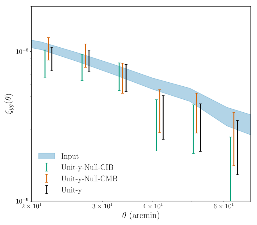
Figure 10: Cross-correlation of reconstructed Compton-$y$ with the halos in Websky mocks for various reconstruction methods. We correlate halos satisfying $0.3<z<0.45$ and $2\times 10^{13}M_{\odot}/h<M_{h}<3\times 10^{13}M_{\odot}/h$. The points labelled ‘input’ correspond to the true halo-$y$ cross-correlation in the absence of any contamination. The other points show the results of applying component separation to simulated sky maps that include the CIB signal. In all cases, we use frequencies 100, 143, 217 and 343 GHz. We find that the choice of unit-$y$, null-CMB leads to no significant bias in the inferred halo-$y$ cross-correlation.

Appendix C Covariance and Multidimensional Parameter constraints

We show the estimated covariance and correlation matrices for the measurements in Fig. 11. As described in §IV.2, we use a jackknife resampling approach to estimating the blocks of the covariance matrix involving the galaxy-$y$ cross-correlation. For the block involving only galaxy-galaxy clustering, we use the theoretical covariance estimate from Krause et al. (2017). We also set to zero the cross redshift-bin covariance for the blocks corresponding to cross-covariance between galaxy-galaxy and galaxy-$y$.

The multidimensional parameter constraints on the galaxy bias and $\langle bP_{e}\rangle$ parameters are shown in Fig. 12 resulting from the MCMC analysis. The MCMC is well converged, and there are no strong degeneracies between the parameters.

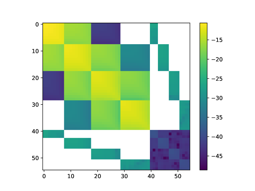
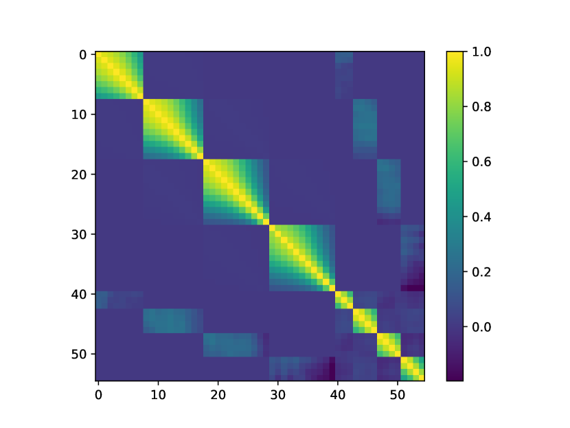
Figure 11: Top panel shows the log of the absolute value of the final covariance matrix. Bottom panel shows the corresponding cross-correlation matrix

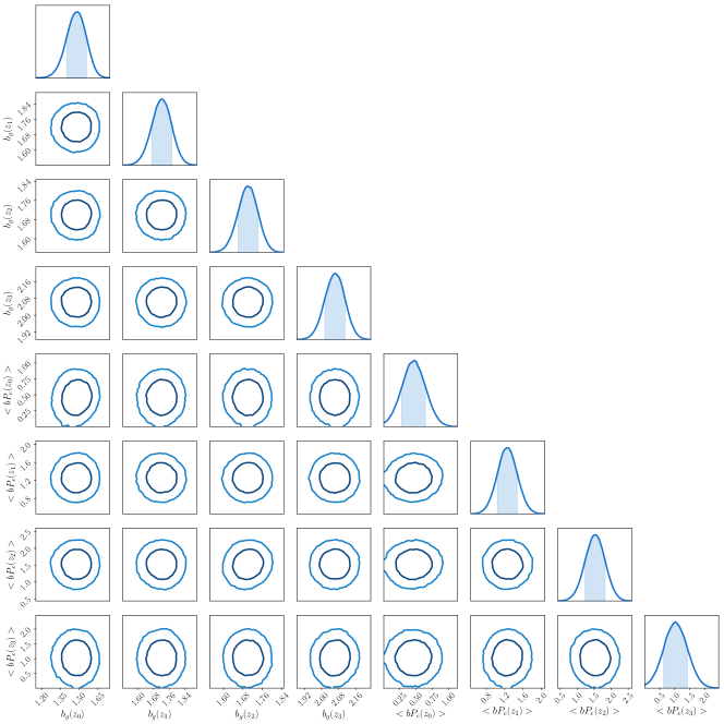
Figure 12: Multi-dimensional parameter constraints from the model fits to data. First four parameters are galaxy bias for each of the four redshift bin used in this analysis and next four are bias weighted pressure corresponding to same bins

References

- Abazajian et al. (2016) Abazajian K. N., et al., 2016, preprint, (arXiv:1610.02743)
- Ade et al. (2019) Ade P., et al., 2019, Journal of Cosmology and Astro-Particle Physics, 2019, 056
- Aghanim et al. (2015) Aghanim P. C. N., Arnaud M., Ashdown M., Aumont J., Baccigalupi C., Banday A. J., Barreiro R. B., 2015, arXiv: 1502.01596v1 [astro-ph.CO 10.1051/0004-6361/201525826, p. 25
- Battaglia et al. (2010) Battaglia N., Bond J. R., Pfrommer C., Sievers J. L., Sijacki D., 2010, ApJ, 725, 91
- Battaglia et al. (2012) Battaglia N., Bond J. R., Pfrommer C., Sievers J. L., 2012, ApJ, 758, 75
- Benson et al. (2014) Benson B. A., et al., 2014, in Millimeter, Submillimeter, and Far-Infrared Detectors and Instrumentation for Astronomy VII. p. 91531P (arXiv:1407.2973), doi:10.1117/12.2057305
- Böhringer & Werner (2010) Böhringer H., Werner N., 2010, A&A Rev., 18, 127
- Bruzual & Charlot (2003) Bruzual G., Charlot S., 2003, MNRAS, 344, 1000
- Carlstrom et al. (2002) Carlstrom J. E., Holder G. P., Reese E. D., 2002, Annual Review of Astronomy and Astrophysics, 40, 643
- Carlstrom et al. (2011) Carlstrom J. E., et al., 2011, Publications of the Astronomical Society of the Pacific, 123, 568
- Carretero et al. (2015) Carretero J., Castander F. J., Gaztañaga E., Crocce M., Fosalba P., 2015, MNRAS, 447, 646
- Cawthon et al. (2018) Cawthon R., et al., 2018, MNRAS, 481, 2427
- Cooray & Sheth (2002) Cooray A., Sheth R., 2002, Phys. Rep., 372, 1
- Crocce et al. (2015) Crocce M., Castander F. J., Gaztañaga E., Fosalba P., Carretero J., 2015, MNRAS, 453, 1513
- DES Collaboration et al. (2017) DES Collaboration et al., 2017, preprint, (arXiv:1708.01530)
- Dark Energy Survey Collaboration et al. (2016) Dark Energy Survey Collaboration et al., 2016, MNRAS, 460, 1270
- DeRose et al. (2019) DeRose J., et al., 2019, arXiv e-prints, p. arXiv:1901.02401
- Delabrouille et al. (2009) Delabrouille J., Cardoso J.-F., Le Jeune M., Betoule M., Fay G., Guilloux F., 2009, A&A, 493, 835
- Delabrouille et al. (2014) Delabrouille J., Cardoso J. F., Jeune M. L., Betoule M., Fay G., Guilloux F., 2014
- Di Matteo et al. (2005) Di Matteo T., Springel V., Hernquist L., 2005, Nature, 433, 604
- Elvin-Poole et al. (2018) Elvin-Poole J., et al., 2018, Phys. Rev. D, 98, 042006
- Evrard (1990) Evrard A. E., 1990, ApJ, 363, 349
- Flaugher et al. (2015) Flaugher B., et al., 2015, The Astronomical Journal, 150, 150
- Foreman-Mackey et al. (2013) Foreman-Mackey D., Hogg D. W., Lang D., Goodman J., 2013, Publications of the Astronomical Society of the Pacific, 125, 306
- Fosalba et al. (2015a) Fosalba P., Gaztañaga E., Castander F. J., Crocce M., 2015a, MNRAS, 447, 1319
- Fosalba et al. (2015b) Fosalba P., Crocce M., Gaztañaga E., Castander F. J., 2015b, MNRAS, 448, 2987
- Greco et al. (2015) Greco J. P., Hill J. C., Spergel D. N., Battaglia N., 2015, ApJ, 808, 151
- Guilloux et al. (2007) Guilloux F., Fay G., Cardoso J.-F., 2007, arXiv e-prints, p. arXiv:0706.2598
- Henderson et al. (2016) Henderson S. W., et al., 2016, Journal of Low Temperature Physics, 184, 772
- Hill & Spergel (2013) Hill J. C., Spergel D. N., 2013, Journal of Cosmology and Astroparticle Physics, 2014, 030
- Hill et al. (2018) Hill J. C., Baxter E. J., Lidz A., Greco J. P., Jain B., 2018, Phys. Rev. D, 97, 083501
- Jarvis et al. (2004) Jarvis M., Bernstein G., Jain B., 2004, MNRAS, 352, 338
- Krause et al. (2017) Krause E., et al., 2017, arXiv e-prints, p. arXiv:1706.09359
- Landy & Szalay (1993) Landy S. D., Szalay A. S., 1993, ApJ, 412, 64
- Le Brun et al. (2015) Le Brun A. M. C., McCarthy I. G., Melin J.-B., 2015, Monthly Notices of the Royal Astronomical Society, 451, 3868
- Limber (1953) Limber D. N., 1953, ApJ, 117, 134
- Loverde & Afshordi (2008) Loverde M., Afshordi N., 2008, Phys. Rev. D, 78, 123506
- MacCrann et al. (2018) MacCrann N., et al., 2018, MNRAS, 480, 4614
- Makiya et al. (2018) Makiya R., Ando S., Komatsu E., 2018, MNRAS, 480, 3928
- Marinucci et al. (2008) Marinucci D., et al., 2008, MNRAS, 383, 539
- Naab & Ostriker (2017) Naab T., Ostriker J. P., 2017, Annual Review of Astronomy and Astrophysics, 55, 59
- Norberg et al. (2009) Norberg P., Baugh C. M., Gaztañaga E., Croton D. J., 2009, MNRAS, 396, 19