Learning Fair Representations via an Adversarial Framework

Abstract.

Fairness has become a central issue for our research community as classification algorithms are adopted in societally critical domains such as recidivism prediction and loan approval. In this work, we consider the potential bias based on protected attributes (e.g., race and gender), and tackle this problem by learning latent representations of individuals that are statistically indistinguishable between protected groups while sufficiently preserving other information for classification. To do that, we develop a minimax adversarial framework with a generator to capture the data distribution and generate latent representations, and a critic to ensure that the distributions across different protected groups are similar. Our framework provides theoretical guarantee with respect to statistical parity and individual fairness. Empirical results on four real-world datasets also show that the learned representation can effectively be used for classification tasks such as credit risk prediction while obstructing information related to protected groups, especially when removing protected attributes is not sufficient for fair classification.

1. Introduction

Consequential decisions in societally critical domains, ranging from criminal justice, to banking, to medicine, are increasingly informed by predictions from machine learning models. These machine learning models heavily rely on historical data and can inherit existing biases, leading to discriminative outcomes. For instance, in the criminal justice system, Angwin et al. (2016) find that African-American defendants tend to be assessed with a higher risk than they actually are compared with white defendants; in online advertisting, a female user may be shown lower-priced products than a male user, even though they have similar preferences (Datta et al., 2015; Sweeney, 2013). As a result, fair machine learning is emerging as a central issue for deploying machine learning models in human society (Holstein et al., 2019).

We focus on the issue of fairness with respect to protected attributes such as gender and race in a classification setting to ensure “fair” decisions across protected groups. However, the formulation of “fairness” is non-trivial and a growing body of research has examined a variety of definitions and developed computational approaches for achieving desired characteristics (Pleiss et al., 2017; Hardt et al., 2016; Agarwal et al., 2018; Hajian and Domingo-Ferrer, 2013; Luong et al., 2011; Calders and Verwer, 2010; Kamishima et al., 2012; Kamiran et al., 2010, 2012a; Hajian and Domingo-Ferrer, 2013; Kamiran and Calders, 2012; Žliobaite et al., 2011; Feldman et al., 2015). For example, statistical parity entails that the proportion of the individuals in a protected group classified as positive instances are identical to the proportion of the whole population, and Kamishima et al. (2012) use regularization techniques to achieve statistical parity. Other popular metrics include false negative rates, false positive rates, and calibration within groups (see Corbett-Davies and Goel (2018) for a recent survey). Here we highlight two important theoretical results: 1) simultaneously satisfying multiple fairness metrics can be challenging and even provably impossible for three intuitive metrics (Kleinberg et al., 2016); 2) Dwork et al. (2012) show that if the distributional distance between features of different groups is small, Lipschitz conditions imply both statistical parity and individual fairness

We build on the theoretical results in Dwork et al. (2012) and propose an adversarial representation learning framework that achieves statistical parity and individual fairness. Specifically, we formulate fairness as an optimization problem of learning representations for individuals, such that given an individual’s latent representation, a task-specific classifier can obtain good performance, while one can hardly distinguish individuals in any protected groups. Our approach reduces the Wasserstein distance between the feature distributions of people in different protected groups through an adversarial framework. Namely, a generator learns the data distribution and transform the original (biased) features into latent representations, while a “critic” ensures the distributions of latent representations are indistinguishable across projected groups.

The advantage of our framework is twofold. First, our framework provides theoretical guarantees on two important fairness metrics, statistical parity and individual fairness. Such guarantees are particularly strong given the impossibility results in Kleinberg et al. (2016). Second, compared to prior work on adversarial learning for fair classification (Edwards and Storkey, 2015; Zhang et al., 2018; Madras et al., 2018), our framework directly minimizes the distributional distance of latent representations between protected groups rather than minimizing the ability to predict protected attributes. Our method effectively blocks the information related to protected attributes and hence ensures fairness properties with any downstream models that satisfy Lipschitz conditions.

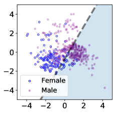
(a) Original features.

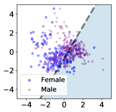
(b) Original features except gender.

(c) Fair Representation.

Figure 1. Illustration of fair representations. Figure 1(a) shows the original features, Figure 1(b) shows the the original features excluding the gender attribute, and Figure 1(c) shows the fair representations learned by our model. The features are scaled and projected into $\mathbb{R}^{2}$ using PCA. The solid orange points represent male individuals, and hallow blue points represent females. The solid lines are decision boundaries by linear classifiers, where the light blue areas are classified as having more than $50,000 annual income, and the white areas are the opposite. 2,000 random samples from the Adult dataset are plotted.

To illustrate the intuition of our fair representations, we present an example from the Adult dataset (Lichman et al., 2013), where individuals are labeled by whether their income exceeds $50,000 per year. We visualize the dataset by projecting the attributes to $\mathbb{R}^{2}$ by PCA in Figure 1. The black dashed line is the decision boundary of logistic regression w.r.t. the label, and different colors indicate different gender. In this dataset, females are less likely to have a high income compared to their male counterparts, and such bias carries over into the predictions from the original features. Based on the original features, the distributional difference between males and females is clear (Figure 1(a)) and the logistic regression classifier gives males about 2.39 (Figure 3(d)) more chances of having a high income. A straightforward strategy to mitigate such bias is to remove the attribute “gender” from the data. However, even after removing “gender”, the distributional difference still exists in Figure 1(b), and males are now 1.95 (Figure 3(d)) more likely to have a high income. This is because the data suffers from “indirect discrimination” (Žliobaite, 2015; Hajian and Domingo-Ferrer, 2013): other attributes relevant to “gender” may still inflict discrimination upon females. This motivates us to reduce both direct and indirect discrimination by learning fair representations of data that are independent of gender. Figure 1(c) showcases our learned fair representations, where one can hardly distinguish males and females as a whole, and males and females are equally likely to have a high income when this representation is used by a learning algorithm.

To further evaluate the effectiveness of our algorithm in promoting fair decision-making, we conduct experiments on four real-world datasets in Section 5. First, we use gender as the protected attribute for all four datasets. Experimental results show that classification is fairer using our learned representations than by using original attributes, with or without the protected attribute, in terms of multiple fairness metrics. Furthermore, we extended our model to the case where the protected attribute is categorical with more than two classes, e.g., race and demonstrate how our method can also be used to discover biases.

Finally, we highlight our contributions as follows:

• We use the Wasserstein Distance to measure if a learned representation is fair and as a result, provide theoretical guarantee for two common formulations of fairness constraints, statistical parity and individual fairness.

• We develop an adversarial framework to incorporate our new metric and learn fair representations for given individuals.

• We validate our proposed framework by conducting extensive experiments on real-world datasets. Using the learned latent representations, we can obtain a competitive prediction performance while ensuring that the protected attributes are unidentifiable. We will release our code upon publication.

2. Related Work

We summarize related work in the following three strands.

Fair representation learning. Most relevant to our work are studies on fair representation learning. Zemel et al. (2013) was the first to propose learning fair intermediate representations: their method involves finding $k$ prototypes in the same space as the input data. Their approach is similar $k$-means, which assigns each sample point to the closest prototype while adding the fairness constraint and classification performance to the optimization objective. However, their representation is inflexible and loses too much information.

Recent advances in generative adversarial networks have also inspired studies that learn fair representations (Edwards and Storkey, 2015; Beutel et al., 2017; Madras et al., 2018). Edwards and Storkey (2015) first made the connection between adversarial and fair machine learning, and Beutel et al. (2017) analyzed Edwards and Storkey’s algorithm and found that their method can be instable when the demographics of the protected attribute are imbalanced. Zhang et al. (2018) used a adversarial agent which attempts to predict the protected attribute solely based on the classifier output; Madras et al. (2018) used an adversary objective based on the learned representations in order to achieve statistical parity and equalized odds. These methods are all based on using a classifier that predicts the protected attribute as the adversarial component.

However, such an adversarial setup requires that any adversary cannot predict the protected attribute, which can be too difficult to optimize in practice. Our method directly reduces the distributional distances between different groups induced by the protected attribute in the latent space. Thus, it is automatically ensured that any classifier cannot predict the protected attribute better than random guessing and the two fairness constraints are satisfied. Hence, with our model, a rather simple architecture is enough for both efficiently preserving information and ensuring fairness constraints, which makes the optimization of our model much easier.

Adversarial learning and autoencoder. Wang et al. (2014) summarizes the framework of autoencoders, and there exists many variations  (Bengio et al., 2013; Kingma and Welling, 2013). Adversarial networks were first proposed by Goodfellow et al. (2014). Most relevant to our work is WGAN proposed by Arjovsky et al. (2017), which replaces the KL-divergence with the Wasserstein Distance, to improve stability of convergence.

Discovering biases. Another important direction we have not discussed is to discover biases in algorithmic systems. Many studies give concrete examples and case analysis of biases in algorithmic systems (Sweeney, 2013; Datta et al., 2015; Roth and Peranson, 1997; Kamiran et al., 2012b; Romei et al., 2013; Mikians et al., 2012). The existence and origin of algorithmic bias and its legal background were thoroughly surveyed by Calders and Žliobaitė (2013); Romei and Ruggieri (2014); Gellert et al. (2013). Several criteria are proposed for quantifying the extent of biases (Luong et al., 2011; Dwork et al., 2012; Zemel et al., 2013; Romei and Ruggieri, 2014; Pedreschi et al., 2012, 2009).

3. Problem Definition

Given a set of individuals $\{u_{1},\cdots,u_{N}\}$, each individual $u_{i}$ is denoted as a triple $(\mathbf{x}_{i},y_{i},p_{i})$, where $\mathbf{x}_{i}\in\mathbb{R}^{d}$ represents their attributes, $y_{i}\in\{0,1\}$ is the label used for the specific relevant classification task, and $p_{i}\in\{0,1\}$ is the protected attribute that we hope to conceal in the classification process.

Indeed, there are some attributes, such as gender, race, age, etc., which should not be used in the decision-making process, because using it would violate fairness and legitimacy of the result, no matter how accurate the model is fitted on the observed data. It is our intention that the protected attributes have no impact on the decision-making process. This process should give due consideration to an individual’s traits and talents instead of a relevant group to which they belong. To this end, simply ignoring the protected attribute alone is not enough, because other attributes are often correlated with the protected attribute, and it is often useful when removing possible bias.

In this section, we consider only binary protected attributes. In Section 4.4, we extended the model to the multi-class scenario and conducted experiments. As such, samples can be categorized into different groups according to their protected attributes. Groups that suffer from discrimination are called protected groups. Furthermore, we define $n_{c}$ as the number of samples that belongs to a particular protected category (i.e., $p_{i}=c$) and denote $U^{(c)}$ as the subset with $p_{i}=c$.

It is natural to assume that some different distributional rules govern the generation of data of the different groups. We define two probability measures over the Borel sets of $\mathbb{R}^{d}$, say $\mu_{0}$ and $\mu_{1}$, as the generator of data with $p_{i}=0$ and $p_{i}=1$, respectively.

Learning fair representations. The goal is to learn a representation vector for each individual in some latent feature space $\mathbb{R}^{k}(k\leq d)$. We define a mapping $f:\mathbb{R}^{d}\rightarrow\mathbb{R}^{k},\mathbf{x}_{i}\mapsto\mathbf{z}_{i}$, where $\mathbf{z}_{i}$ is the desired representation of $\mathbf{x}_{i}$. Each component of $\mathbf{z}_{i}$ is real-valued and continuous. Let $\mathbf{Z}=[\mathbf{z}_{1},\ldots,\mathbf{z}_{n}]$, for a classification task, we first map $\mathbf{X}=[\mathbf{x}_{1},\ldots,\mathbf{x}_{n}]$ to $\mathbf{Z}$, and then map $\mathbf{Z}$ to $\mathbf{Y}=[y_{1},\ldots,y_{n}]$.

Usually, a good representation vector is expected to preserve most of the information from the original vector. However, when fairness is at risk, we wish to further impose some constraints on the distribution of instances in the feature space, such that statistical parity and individual fairness are met.

Fairness constraints. We define $\Psi:\mathbb{R}^{k}\rightarrow[0,1]$ as the classifier that assigns each individual a classification score. In this paper, we discuss two popular realizations of fairness constraints, as listed below. Similar ideas are also discussed in Dwork et al. (2012); Corbett-Davies et al. (2017); Zemel et al. (2013).

• Statistical parity (Corbett-Davies et al. (2017)): all groups with the protected attribute receive similar expected classification scores, i.e., $\mathbb{E}[\Psi(\mathbf{Z})|P]=\mathbb{E}[\Psi(\mathbf{Z})]$;

• Individual fairness (Dwork et al. (2012)): similar individuals receive similar scores, i.e., $|\Psi(\mathbf{z}_{1})-\Psi(\mathbf{z}_{2})|\leq K\|\mathbf{z}_{1}-\mathbf{z}_{2}\|_{2}$. In other words, the difference between the classification scores is bounded by the difference between individual features.

These are two representative definitions of algorithmic fairness from relevant literature. Throughout the paper, we use these definitions to refer to their respective notions of fairness.

4. Our Approach

In this section, we propose a minimax adversarial gaming framework to learn the fair representations of the relevant individuals. Intuitively, to meet fairness constants, the fair representations are those that lose the information about the protected attributes while preserving as much of the other information of that individual as possible. In other words,

• It contains little or no information about the protected attributes. Therefore, it is difficult to distinguish the protected groups from the others according to fair representations.

• Still, it can preserve as much information as possible except for the protected attribute. , except for the protected attribute, as possible.

4.1. Framework

To hide the protected attributes, we impose the constraint that the conditional distributions given the protected attributes are identical across the feature space. Therefore, we define a fairness metric to evaluate the quality of a learned representation:

(1) $$L=L_{A}+\alpha L_{D}$$

The proposed metric $L$ comprises of two parts: $L_{A}$ is the information loss term, evaluating how much information the embedding mapping $f$ has not preserved compared with the original feature matrix; and $L_{D}$ measures how close the distributions over different groups of the protected attribute (i.e., $\mu_{0}$ and $\mu_{1}$) are in the latent space. We expect that a fair representation has small-valued $L_{A}$ and $L_{D}$. The hyperparameter $\alpha$ controls the trade-off of the system.

Later in this section, we introduce the relationship between the proposed fair metric $L$ and the fairness constraints theoretically. Prior to that, we present the overall structure of our approach.

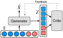
Figure 2. Structure of our proposed model. Red circles (square) represent $\mathbf{X}$ ($\mathbf{U}$) of individuals in protected group, while blue ones indicate that of other individuals.

Overall, as Figure 2 shows, the proposed framework consists of two components: 1) the generator, which takes individual features $\mathbf{X}$ as the input, learns representations $\mathbf{Z}$ of individuals, and recovers individual features according to the learned representations and 2) the critic, which measures the distance between $\mu_{0}$ and $\mu_{1}$. The critic guides the learning process of the generator, ensuring that the different values of the protected attributes can hardly be distinguished in the representation space while the generator provides the representations of individuals. Note that the goal of the critic and the generator correspond to $L_{D}$ and $L_{A}$ respectively. We next introduce how to implement the critic and the generator.

Generator. The generator aims to generate data representations. In this paper, we use an autoencoder as an example to implement the generator and learn the representations of the individuals. In particular, the autoencoder comprises of two multilayer perceptrons: the encoder $f$, which takes data as input and produces latent representation; and the decoder $g$, which operates inversely. We define $L_{A}$ in (1) as the mean square error between $X$ and $g(f(X))$, since $g\circ f$ tries to reproduce $X$ when $X$ is given.

For simplicity and interpretability, we use a single linear layer for both the encoder and the decoder. Thus, the latent features are simply linear transformations of the original attributes. We denote, therefore, $\mathbf{Z}=\mathbf{X}\mathbf{A}$, where $\mathbf{A}\in\mathbb{R}^{d\times k}$ defines a linear mapping to the feature space.

$\mu_{0},\mu_{1}$ and the encoder $f$ induces probability measures on the latent space $\mathbb{R}^{k}$, $f(\mu_{0})$ and $f(\mu_{1})$, representing the distributions of data with different $p_{i}$’s in the latent space. Since we are always concerned with the distributions on the latent space, for notational convenience, in the following paper, we use $\mu_{0},\mu_{1}$ themselves to refer to the probability measures on the latent space without specifying $f$.

Critic. The goal of the critic is to keep the protected attributes similar for different groups. To calculate $L_{D}$, we measure the distance between $\mu_{0}$ and $\mu_{1}$ by the Wasserstein Distance, or the Earth Mover’s Distance (EMD), as follows:

(2) $$L_{D}=D_{W}(\mu_{0},\mu_{1})=\inf_{\gamma\in\Gamma(\mu_{0},\mu_{1})}\left(\int_{\mathbb{R}^{k}\times\mathbb{R}^{k}}\|\mathbf{z}_{0}-\mathbf{z}_{1}\|_{2}d\gamma(\mathbf{z}_{0},\mathbf{z}_{1})\right)$$

The sole context is Euclidean metric space. $\mu_{0},\mu_{1}$ are two probability measures defined on $\mathbb{R}^{k}$, which represent the distribution of data with different $p_{i}$ in the latent space. $\Gamma(\mu_{0},\mu_{1})$ is the collection of all probability measures on $\mathbb{R}^{k}\times\mathbb{R}^{k}$, with two marginal distributions of $\mu_{0}$ and $\mu_{1}$ respectively.

This definition is based on the intuition of optimal transport, i.e., the minimum “weight” that needs to be transferred to transform the density of $\mu_{0}$ into $\mu_{1}$.

Unfortunately, the computation of (2) is intractable. Instead, we use the Kantorovich-Rubinstein Duality (Villani, 2008):

(3) $$D_{W}(\mu_{0},\mu_{1})=\frac{1}{K}\sup_{\|D\|_{L}\leq K}\mathbb{E}_{\mathbf{z}\sim\mu_{0}}D(\mathbf{z})-\mathbb{E}_{\mathbf{z}\sim\mu_{1}}D(\mathbf{z})$$

Here, $D$ is our critic, which is taken across all functions $\mathbb{R}^{k}\rightarrow\mathbb{R}$ satisfying the Lipschitz condition. The Lipschitz condition provides that $|D(\mathbf{z}_{0})-D(\mathbf{z}_{1})|\leq K\|\mathbf{z}_{0}-\mathbf{z}_{1}\|_{2}$. $K$ here is called the Lipschitz constant, denoted by $\|D\|_{L}$, as in (3).

In this paper, we use a linear mapping to implement the critic $D$, which is used to approximate the EMD. This approach, in turn, provides a useful gradient for the generator to ensure that the EMD is close to zero. The efficiency of this approach is tested in (Arjovsky et al., 2017). Therefore, our objective can be written in the following minimax form:

(4) $$\min_{A}{}\max_{D}{}L(A,D) = L_{A}+\alpha L_{D}$$

Here, $L_{A}$ is the information loss term, and $L_{D}$ is the approximation of EMD provided by the critic $D$. $L_{D}$ is first maximized to ensure good approximation and to yield a usable gradient for the generator. Then the generator $A$ minimizes both the information loss and the EMD distance. Note that the critic is a real-valued linear mapping, and is therefore a vector in $\mathbb{R}^{k}$.

To ensure Lipschitz condition in general multilayer neural networks, we may clamp the model parameters to the range of $[-c,c]$, where $c$ is a positive real number. This is the approach practiced by (Arjovsky et al., 2017). Since neural networks are differentiable, this ensures bounded first-order derivative and therefore the Lipschitz condition.

4.2. Relation to Fairness Constraints

Dwork et al. (2012) explained that statistical parity and individual fairness can be jointly achieved if the Wasserstein Distance between two groups is small. Here, we give concrete reasons for why we have selected the Wasserstein Distance as an optimization objective by showing that it may ensure the fairness of the classification results on the learned features for a wide range of well-conditioned classifiers.

Definition 0.

Suppose $\Psi$ is a mapping $\mathbb{R}^{k}\rightarrow\mathbb{R}$ satisfying

$$|\Psi(\mathbf{z}_{0})-\Psi(\mathbf{z}_{1})|\leq K\|\mathbf{z}_{0}-\mathbf{z}_{1}\|_{2}$$

where $K$ is a positive constant, then we say $\Psi$ satisfies the Lipschitz condition, and denote it by $\|\Psi\|_{L}\leq K$, where $K$ is called the Lipschitz constant.

Theorem 2.

If $\Psi$ is a mapping $\mathbb{R}^{k}\rightarrow\mathbb{R}$ representing a classifier, and $\|\Psi\|_{L}\leq K$, $\mu_{0},\mu_{1}$ are two probability measures defined over $\mathbb{R}^{k}$ that generates the two categories of the protected attribute, then the individual fairness is bounded by the Lipschitz constant as is the Definition 1. Furthermore, the statistical parity is bounded by the Wasserstein disance and the Lipschitz constant:

(5) $$|\mathbb{E}_{\mathbf{z}\sim\mu_{0}}\Psi(\mathbf{z})-\mathbb{E}_{\mathbf{z}\sim\mu_{1}}\Psi(\mathbf{z})|\leq KD_{W}(\mu_{0},\mu_{1})$$

Theorem 5 shows how to principally ensure both statistical parity and individual fairness. Clamping parameters or $\ell_{2}$ weight decay both reduce the Lipschitz constant of the classifier. (5) shows that by reducing the EMD distance, enforcing individual fairness achieves statistical parity as well.

Algorithm 1 The learning algorithm.

1:  Normalize the input data

2:  for $n_{iter}$ training epochs do

3:     Sample a batch of data $x_{0}^{(i)},\ldots,x_{L}^{(i)}$ from $U^{(i)}$ for $i=0,1$

4:     while not converged do

5:        Update the parameters of the critic:

$$L_{D}=\frac{1}{L}\sum_{i=1}^{L}{D(f(x_{i}^{(0)}))-D(f(x_{i}^{(1)}))}$$

$$\theta_{D}=\theta_{D}+\mu\frac{\partial}{\partial\theta_{D}}L_{D}$$

6:        Clipping the values of $\theta_{D}$ to the range of $[-c,c]$

7:     end while

8:     Update the parameters of the autoencoder:

$$L_{A}=\frac{1}{L}\sum_{i=1}^{2}\sum_{j=1}^{L}(g(f(x_{j}^{(i)}))-x_{j}^{(i)})$$

$$L_{D}=\frac{1}{L}\sum_{i=1}^{L}{D(f(x_{i}^{(0)}))-D(f(x_{i}^{(1)}))}$$

$$\theta_{A}=\theta_{A}-\mu\frac{\partial}{\partial\theta_{A}}(L_{A}+\alpha L_{D})$$

9:  end for

4.3. Model Learning

By putting everything together, we obtain our model with the dynamics as a minimax adversarial game:

$$\min_{A}{}\max_{D}{}L(A,D) = L_{A}+\alpha L_{D}$$

$$= \frac{1}{n}\sum_{i=1}^{n}(g(f(x_{i}))-x_{i})^{2}$$

$$+ \frac{1}{n_{0}n_{1}}\sum_{i}\sum_{j}D(f(x_{i}^{(0)}))-D(f(x^{(1)}_{j}))$$

Let $\theta_{A}$ and $\theta_{D}$ indicate the parameters of the autoencoder and the critic respectively, we introduce how to learn $\theta_{A}$, $\theta_{D}$, and the latent representation $\mathbf{U}$ simultaneously. Algorithm 1 is the training process. First, the critic is trained sufficiently until the terminal condition is met. In our experiments, we keep training the critic until the change in value is less than $1e-3$. Then, the autoencoder is trained to minimize the MSE loss and the EMD by using the gradients provided by the critic.

4.4. Beyond Binary Protected Attributes

Previously, we assume the protected attribute is binary, i.e. gender. In practice, protected attributes are often multi-class categorical variables. Suppose the protected attribute is converted to numeric representation $P=0,1,\ldots,n_{p}-1$, where $n_{p}$ is the number of categories that the protected attribute may assume.

Our original formulation of the model in the binary case may be viewed as an approximation of the following objective:

(6) $$\min \frac{1}{n}\sum_{i}(g(f(x_{i}))-x_{i})^{2}$$

$$\operatorname{s.t.} D_{W}(f(U^{(0)}),f(U^{(1)}))=0$$

where $U^{(j)}$ represents the collection of samples which satisfies $p_{i}=j$, $j=0,1$.

The direct extension to the multi-class case would be adding as many constraints as to ensure that the distributional difference between any two classes is zero. However, this would add $\binom{p}{2}$ constraints. Therefore, it is more desirable to define the multi-class objective in a “one-vs-rest” manner. We denote $U^{(-j)}$ as all the samples that $p_{i}\neq j$. The multi-class objective is then

(7) $$\min \frac{1}{n}\sum_{i}(g(f(x_{i}))-x_{i})^{2}$$

$$\operatorname{s.t.} D_{W}(f(U^{(j)}),f(U^{(-j)}))=0, j=0,\ldots,n_{p}-1$$

Intuitively, this adds $p$ constraints and $p$ critics that are needed to approximate the Wasserstein distances. However, we discovered in our experiments that using only one linear critic for all the distributions has similar performance comparing with using one linear critic for each of the distributions. Therefore, we used only one linear critic to approximate the distributions.

Implementation note. For a given $i$, a training iteration is exactly like Algorithm 1, replacing $U^{(0)},U^{(1)}$ with $U^{(j)},U^{(-j)}$. In practice, to ensure that each class’s distributional difference with the rest is sufficiently optimized, we train for one specific class for 10 iterations before we turn to the next class.

5. Experimental Setup

In this section, we describe the datasets, baselines, and evaluation metrics used in our experiments.

Datasets. We conduct experiments on four real-world datasets:

• Adult (Lichman et al., 2013). This dataset is extracted from the 1994 Census database. Each sample represents an individual and is classified based on whether the individual’s annual income exceeds $50,000.

• Statlog (Lichman et al., 2013). This is the German credit data. In this dataset, every individual is classified as either good or bad in terms of credit risks.

• Fraud. This dataset is provided by PPDai, the largest unsecured micro-credit loan platform in China. It consists of over 200,000 registered users and over 37 million call logs between them. Each user’s features are extracted from their basic information (e.g., age, gender, education, etc.) and call behavior (e.g., call number, call duration, etc.). We aim to determine each user’s credit risk by deducing whether they will default pn a loan for more than 90 days.

• Investor. This dataset is provided by PPDai. It consists of almost 10,000 registered investors, and each of which is classified as investing over $73,000. The attributes are the user’s basic information (e.g., age, gender, residential place, house price) and behavior (e.g., frequency of use of the app, etc.)

For all datasets, we choose Gender as the protected attribute. Female is the protected group in our tasks. Note that although gender is a binary attribute in all the four datasets, we recognize that gender may not be binary.

	Samples	Attributes	Protected (%)	Positive (%)
Adult	48,842	14	33.0	24.0
Statlog	1,000	20	15.0	30.0
Fraud	205,835	37	21.1	10.0
Investor	9,827	6	42.0	11.0

Table 1. Statistics concerning datasets. The columns are the numbers of samples and attributes and percentages of protected group (female) and positive samples.

Tasks. In our experiments, we first learn the latent representations according to the given feature matrix $\mathbf{X}$, then we conduct the following classification tasks to validate the effectiveness of the learned representations:

• Task I. We use the representation methods to learn the latent features of the data and estimate the information loss by MSE and the distributional distance between different groups of the protected attribute.

• Task II. We further use the learned latent features to classify against the data label and examine the size of performance drop and whether the results meet fairness constraints.

Baseline methods. In our experiments, we employ and compare the following different methods for representation learning.

• Original. This method directly uses all features to train a classifier for task I.

• Original-P. This process employs all features except for the protected one to train the classifier.

• AutoEncoder. This process uses an autoencoder to learn representations according to all features.

• AutoEncoder-P. This method uses an autoencoder to learn representations according to all features but the protected one.

• LFR. This is a model for learning fair representations that was proposed by (Zemel et al., 2013). In this method, instances are assigned to certain prototypes as latent representations. We use the parameters advised by the authors (Zemel et al., 2013).

• NRL. This is the proposed fair representation learning method.

We also have compared NRL with the methods proposed by Madras et al. (2018) and Edwards and Storkey (2015). However, we omit the detailed results considering their unstable performance. More specifically, these two methods often require a more complex network architecture than ours. In addition, when using a three-layer neural network for autoencoder and the adversary on the Adult dataset, we found the adversary in Madras et al. (2018) and Edwards and Storkey (2015)’s model indeed cannot predict the protected attribute. However, after the representation is learned, a classifier of the same architecture usually separates well the protected groups.

	Adult	Statlog	Fraud	Investor
AutoEncoder	0.02	0.02	0.02	0.04
AutoEncoder-P	0.05	0.02	0.09	0.15
LFR	1.12	1.17	0.86	1.10
NRL	0.10	0.15	0.21	0.06

Table 2. MSE loss when reconstructing the original features. Lower values indicate less information loss of the corresponding representation of the original data.

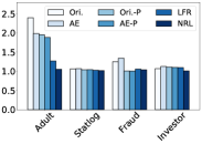
(a) Statistical Parity

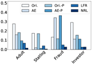
(b) EMD Distance

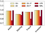
(c) Consistency

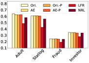
(d) Classification (F1-score)

Figure 3. Evaluation of fairness and classification performance. Ori., AE are short for Original and AutoEncoder. For statistical parity and EMD distance, lower values indicate fairer performance. For consistency, higher scores suggest better results in terms of individual fairness. For Classification, higher scores indicate better performance.

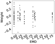
(a) Adult

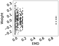
(b) Statlog

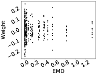
(c) Fraud

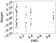
(d) Investor

Figure 4. EMD distance and the weight of the linear encoder. The x-axis is the EMD distance of each individual features between the protected groups. The y-axis is the weight corresponding to the feature in the linear encoders. The higher the absolute value, the more importance the model gives the feature in the representation. It can be observed that as the EMD increases, the weight converges to zero, indicating that the model is more reluctant in using that feature in the representation.

Methods of evaluation. We evaluate the quality of the representation learning using the following metrics:

• The mean square error of the autoencoder, which estimates the information loss of the representation.

• The EMD distance between the representations of different groups.

In addition, in order to investigate the actual effect of our method, classification based on the learned latent representations is also studied. To obtain the classification results, we employ RLR($\ell_{2}$-regularized Logistic Regression, also known as the ridge logistic regression) on $\mathbf{X}$ and $\mathbf{Z}$. The following metrics are used to quantify the quality of classification.

• Classification performance against labels, evaluated by the F1-score. F1-score is calculated by the harmonic average of the precision and recall scores of the prediction.

• The statistical parity score of the classification result against labels, defined as

  $$\frac{\max{(\frac{1}{n_{0}}\sum_{p_{i}=0}\Psi(\mathbf{z}_{i}),\frac{1}{n_{1}}\sum_{p_{i}=1}\Psi(\mathbf{z}_{i}))}}{\min{(\frac{1}{n_{0}}\sum_{p_{i}=0}\Psi(\mathbf{z}_{i}),\frac{1}{n_{1}}\sum_{p_{i}=1}\Psi(\mathbf{z}_{i}))}}$$

• Consistency score of the classification, defined as

  $$yNN=1-\frac{1}{n}\sum_{i=1}^{n}\left|\hat{y}_{i}-\frac{1}{k}\sum_{j\in kNN(\mathbf{x}_{i})}\hat{y}_{j}\right|$$

  This equation evaluates the average differences in classification scores between a point and its $k$-nearest neighbors. A similar calculation is also used in (Zemel et al., 2013). In our experiments, we use $k=1$.

Specifically, to evaluate performance, fair representations are first learned and then fixed. On the learned latent features (or the original features, if no representation is learned), the EMD distance between the groups of the protected attribute and the MSE reconstruction loss are computed.

Then, we train a logistic regression on the latent features to predict labels of data. The logistic regression predicts for each sample a score between 0 and 1 representing its probability of being positively labeled. Using the predicted score, the statistical parity score and the consistency score are calculated.

6. Experimental Results

We first compare our model performance with other approaches using a binary gender attribute, and then extend this to multi-class categorical variables. We further show how our models can be used to discover bias in the dataset.

6.1. Model Performance

Since we attempt to impose fairness constraints, our method is necessarily outperformed in classification by methods without consideration of fairness, including Original, Original-P, AutoEnecoder, and Autoencoder-P. However, the advantage of our method is twofold: 1) it better satisfies fairness constraints than methods without consideration of fairness; 2) it preserves more information and better satisfies fairness constraints than prior approaches, namely, LFR.

Reconstruction loss. Table 2 shows the MSE loss of reconstructing the original features. As we expected, NRL sacrifices performance in information preservation at the cost of enforcing the distributions between two groups being identical, compared to AutoEncoder and AutoEncoder-P. However, NRL preserves much more information than LFR.

Fairness constraints in classification. Figure 3 shows the metrics to evaluate fairness, including the statistical parity score, the EMD distance, and the consistency score. For the former two metrics, lower values indicate better results: lower statistical parity means that the classification has no preference for one category of the protected attribute over the other; lower EMD distance indicates that the information of the protected attribute is better obstructed. For consistency, higher values are better since they capture individual fairness of the classification: similar samples are treated similarly.

NRL consistently provides the best performance in all fairness constraints. We note that AutoEncoder and AutoEncoder-P are sometimes sufficient for achieving strong performance in statistical parity and consistency (Fraud and Investor), because both of these metrics rely on predictions and gender does not really matter in these prediction tasks. In comparison, LFR is not even competitive in these easy cases.

Figure 3(d) shows the cost of fairness. Since we actively loses any information relevant to the protected attribute which is often correlated to the label, the performance in classification inevitability drops compared to methods without considering fairness. However, our method is better compared to LFR, indicating better information preservation, consistent to results in Table 2. Our results suggest that our method can serve as a benchmark to test whether simply approaches such as AE-P and Original-P are enough for achieving desired fairness constraints.

Our experiments evidence that in most cases, simply removing the protected attribute is insufficient. In three of the four datasets, AE-P and Original-P cannot be fairer than NRL. For the Investor dataset, AE-P obtains even lower F1-score and a higher MSE loss.

The Fraud dataset deserves special attention: its statistical parity and consistency is already low enough due to the removal of the protected attribute. Representations learned by NRL and LFR could not be fairer than in the original dataset with the protected attribute removed. Although removing the attribute cannot keep the EMD low, if one is concerned only with classification results, such a simple modification is fair.

How fair representations are generated. It is also of crucial interest that how the model chooses to represent the data. In this section, we give some concrete examples to illustrate how the model learns the proper representation of data that is fair.

For each individual feature of a dataset, we explored the relationship between EMD of that feature across the protected groups and the weight of that feature in the linear encoder. We scatter-plotted the EMD and the weights in Figure 4. One may observe the trend that the linear encoder tends to assign smaller weights in terms of absolute value to features with higher EMD. Since features with higher EMD contribute more to the difference of the joint distribution of all features, it is an empirical evidence that the linear encoder attempts to suppress information related to the protected attribute with the help of the critic.

6.2. Multiclass Protected Attributes

We take the race for an example of a multi-class protected attribute. In Adult dataset, the feature ”race” may take as many as five categories: “White”, “Asian-Pac-Islander”, “Amer-Indian-Eskimo”, “Other”, and “Black”.

For model implementation and parameters in this experiment, the encoder is a three-layer neural network with ReLU nonlinearity. The dimensions of all the hidden layers and the output layer are 10. The decoder is the reversal of the encoder. Finally, the critic is a linear mapping to $\mathbb{R}$, as in previous univariate experiments, and the weight of the loss, $\alpha$, is set as 1000.

For evaluation, the metric which measures the statistical fairness of a prediction, statistical parity, can be thus defined in the multi-class case:

(8) $$\frac{\max_{1\leq i\leq 0n_{p}-1}(\frac{1}{n_{j}}\sum_{p_{i}=j}\Phi(\mathbf{z}_{i}))}{\min_{1\leq i\leq n_{p}-1}(\frac{1}{n_{j}}\sum_{p_{i}=j}\Phi(\mathbf{z}_{i}))}$$

which is the ratio of the maximum to the minimum of the average predicted scores of each class derived by the protected attribute.

Originally, the F1-score of the classification task is as high as 0.64, as indicated in Figure 3(d) Through our learned representation, the F1-score is dropped to 0.42 at the cost of fairness. This is lower than shown in Figure 3(d), indicating that race is more costly than gender when concealed. As a comparison, we also trained vanilla autoencoder on the Adult dataset, with the same architectures for the encoder and the decoder. However, it is hard to converge to a more efficient representation than a simple linear autoencoder, and the average of our attempts yields 1.9 MSE and 0.530 F1 score. Therefore, we also trained a linear autoencoder for comparison.

Experiment results are listed in Table 3, in which we listed two metrics: average prediction score, obtained by a regularized linear classifier based on specific representations; and one-vs-rest EMD, obtained by calculating the distribution difference between one specific class and all others. Using the average prediction score, we may compute the statistical parity for the four methods: 1.70 for original features, 1.77 for multilayer autoencoder, 2.18 for linear autoencoder, and 1.01 for NRL. This indicates that NRL may efficiently prevent discrimination when the protected attribute is multiclass.

One should note that when race information is not hindered by NRL, all other three methods tend to assign lower probabilities of high income to groups of American-Indian-Eskimos and Blacks. This reflects that such discriminatory tendency exists in the data. Our model shows an alternative reality: what would happen if all except race is considered? In Table 3, we see that the probabilities across ethnic groups are leveled around 0.24, a rather high probability, and is close to the White and Asian-Pacific-Islanders, as predicted by original features. The results may shed light on how the economic status of some individuals or ethnic groups as a whole would have been were they not discriminated based on their race.

Metric	Method	AIE	API	Black	Other	White
Avg. Score	Ori.	0.185	0.261	0.153	0.160	0.255
	MAE	0.164	0.291	0.174	0.178	0.249
	LAE	0.359	0.544	0.280	0.613	0.314
	NRL	0.239	0.240	0.238	0.237	0.239
1vsR EMD	Ori.	0.468	0.430	0.281	0.418	0.274
	MAE	0.097	0.098	0.096	0.151	0.075
	LAE	0.164	0.291	0.174	0.178	0.249
	NRL	0.001	0.001	0.002	0.002	0.0017

Table 3. Results for multiclass protected attribute. We listed two metrics for fairness: Avg. Score, which stands for average prediction score, and 1vsR EMD, which stands for one-vs-rest EMD distance. AIE stands for Asian-Indian-Eskimo, and API stands for Asian-Pac-Islander. Four methods are considered: original features, MAE (multilayer autoencoder), LAE (linear autoencoder), and our approach.

6.3. Discovering Biases

Another important problem in the field of algorithmic bias is to discover potential biases. We have so far presented some concrete examples of how the model can “correct” the labels of some females whose labels are “unfairly” negative, while these females have similar male counterparts with positive labels. To see if our model can be used for discovering biases, we explicitly “discriminate” some females by flipping their labels. Specifically, we match each male to its nearest female in terms of Euclidean distance and select the pairs in which both the male and female are positively labeled. We use two approaches to examine the robustness of our framework to such added discrimination: 1) whether we can predict the real label; 2) whether we can detect such discrimination.

Detecting flipped labels. We apply a linear classifier to both our learned representation and the original features. The regularization strength for each classifier is tuned to maximize the proportion of which the flipped labels are corrected. For Adult dataset, 1399 such pairs are selected, and the same amount of female’s labels are manually changed to be negative. Based on our learned representation, 84.4% of the flipped females are predicted as positive by a linear classifier, while on the original features, only 40.6% are. Similarly, 93 pairs are selected for Statlog dataset, and learning on our representation corrects 46.2% of the flipped labels, while on the original features, only 8.6% are successfully classified as positive.

Locating discriminated individuals. The problem of locating discriminated individuals may also be conveniently formulated as locating “mislabeled” samples due to the influence of the protected attribute that ought to have no influence. In practice, an important problem is how to efficiently locate samples that are probably mislabeled, and human experts may proceed to check the labels in detail. In our experiment setting, it is desirable to locate the females whose labels we manually flipped.

An individual is likely to be discriminated or mislabeled if when the protected attribute is not considered, he or she has a high prediction score compared to when the protected attribute is considered. Suppose the prediction score based on original features is $p_{o}$ and the score based on our fair representation is $p_{f}$. We define the following statistics to quantify the “strength” of discrimination against an individual as follows:

(9) $$s_{d}=1-\frac{p_{o}}{p_{f}}$$

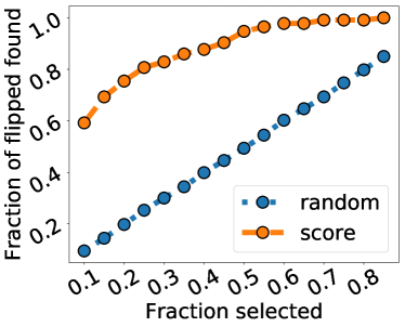
(a) Adult

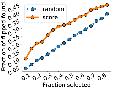
(b) Statlog

Figure 5. Locating discriminated individuals. The x-axis is the fraction of females selected, and the y-axis is the fraction of “discriminated” (flipped) females discovered.

Then we sort the female individuals by $s_{d}$ in descending order, and check the proportion of flipped females among females with the highest $s_{d}$. The results in Adult and Stalog are in Figure 5. Individuals identified with high $s_{d}$ are clearly much more likely to be these “discriminated” ones, compared to a random baseline.

7. Conclusion

In this paper, we proposed learning a latent representation of attributes that achieves fairness by obstructing information concerning a protected attribute as much as possible, while preserving other useful information. Our method pre-processes the data and removes both direct and indirect discrimination for downstream tasks. We formulate this problem in a minimax adversarial framework by learning a transformation of features such that the distributions between different groups of the protected attribute, e.g., male and female, are indistinguishable. This framework provides theoretical guarantee on statistical parity and individual fairness, and also achieves strong empirical results on four real-world datasets. We also note that for some tasks where protected attributes do not play any role, it seems sufficient to remove the protected attributes. Our method can be used as a benchmark to detect these cases.

For future work, it is interesting to explore if our approach can be extended to applications beyond fairness. For example, it is often useful to infer the counterfactual scenario: what would happen when one variable is absence? With that variable as the protected attribute, one may further analyze the problem. Another promising direction is to further consider continuous protected attributes or discrete ones with a large value range, such as age.

Appendix A Supplementary Materials

A.1. Model Parameters.

We employ a simple linear layer for the encoder, the decoder, and the critic. Thus, the representation $\mathbf{U}$ is simply a linear transformation of the input $\mathbf{X}$.

The continuous variables of all four datasets are scaled by their mean and standard variance. For NRL and AE, the dimension for the feature space is 12 for Adult, 23 for Statlog, 30 for Fraud, and 5 for Investor. The dimension for AE-P is reduced by one. $\alpha$ for NRL is 10 for Adult, Fraud, and Investor, and 100 for Statlog. The inverse of the regularization strength for logistic regression for all datasets is 0.01.

A.2. Details of Evaluation.

We used NRL to learn fair representations on the entire dataset. After that, two classifiers are trained on the learned representations to evaluate performance as described in Section 4.

For each classifier, the parameters are trained on 70% of the data, i.e. the training set, randomly and uniformly sampled from the whole dataset. The scores are calculated on the remaining test set. This process is repeated 5 times and the scores are averaged.

The whole process from training fair representations to training classifiers is repeated 10 times and the final displayed scores in Table 2 and Table LABEL:table:metric:cls is the average of the 10 repeated experiments.

A.3. Parameter Analysis

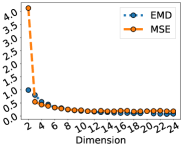
(a) Statlog

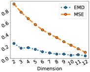
(b) Adult

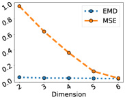
(c) Investor

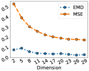
(d) Fraud

Figure 6. Dimension and MSE and EMD. Generally, as the dimension increases, both MSE and EMD reduces.

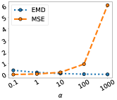
(a) Statlog

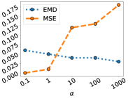
(b) Adult

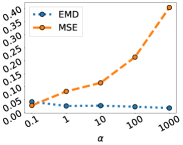
(c) Investor

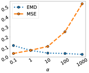
(d) Fraud

Figure 7. Parameter $\alpha$ and MSE and EMD. $\alpha$ controls the strength of fairness constraints; higher $\alpha$ enforces the model to generate fairer representation by reducing EMD.

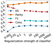
(a) Statlog

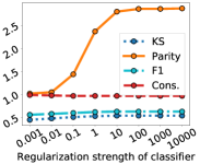
(b) Adult

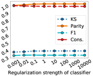
(c) Investor

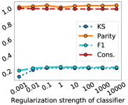
(d) Fraud

Figure 8. Inverse of regularization strength of the classifier and the performance. The x-axis is the inverse of the regularization strength; higher values means weaker regularization. The right-most value is proximal to the case where there is no regularization at all.

We analyzed the influence of several hyperparameters, including the dimension of the feature space, the trade-off parameter $\alpha$, and the regularization strength of the linear classifier, on information preservation, classification performance, and fairness. When studying one of them in particular, other hyperparameters are fixed, as described earlier in this section.

Figure 6 shows the influence of dimension. As we observed in experiments, a sufficiently high dimension, usually close to the original number of attributes, helps MSE and EMD reduction. In a higher dimension, MSE is more easily reduced, which makes it easier at reducing EMD as well. Therefore, we would suggest a sufficiently high dimension, often close to the dimension of the original attributes, unless there is need for dimensionality reduction.

Figure 7 shows the trade-off between fairness and information preservation, controlled by $\alpha$. Figure 8 shows the influence of the regularization strength of the classifier, which maps the samples in our learned feature space to the classification scores. Except for Adult, the influence of the regularization strength is mild, but the classification is still fairer when the regularization is stronger. Furthermore, the cost of achieving fairness in terms of classification results is not expensive.

References

- (1)
- Agarwal et al. (2018) Alekh Agarwal, Alina Beygelzimer, Miroslav Dudík, John Langford, and Hanna Wallach. 2018. A reductions approach to fair classification. In Proceedings of ICML.
- Angwin et al. (2016) Julia Angwin, Jeff Larson, Surya Mattu, and Lauren Kirchner. 2016. Machine bias: There’s software used across the country to predict future criminals and it’s biased against blacks. ProPublica (2016).
- Arjovsky et al. (2017) Martin Arjovsky, Soumith Chintala, and Léon Bottou. 2017. Wasserstein GAN. arXiv preprint arXiv:1701.07875 (2017).
- Bengio et al. (2013) Yoshua Bengio, Li Yao, Guillaume Alain, and Pascal Vincent. 2013. Generalized denoising auto-encoders as generative models. In Advances in Neural Information Processing Systems. 899–907.
- Beutel et al. (2017) Alex Beutel, Jilin Chen, Zhe Zhao, and Ed H Chi. 2017. Data decisions and theoretical implications when adversarially learning fair representations. arXiv preprint arXiv:1707.00075 (2017).
- Calders and Verwer (2010) Toon Calders and Sicco Verwer. 2010. Three naive Bayes approaches for discrimination-free classification. Data Mining and Knowledge Discovery 21, 2 (2010), 277–292.
- Calders and Žliobaitė (2013) Toon Calders and Indrė Žliobaitė. 2013. Why unbiased computational processes can lead to discriminative decision procedures. In Discrimination and privacy in the information society. Springer, 43–57.
- Chouldechova (2017) Alexandra Chouldechova. 2017. Fair prediction with disparate impact: A study of bias in recidivism prediction instruments. Big data 5, 2 (2017), 153–163.
- Corbett-Davies and Goel (2018) Sam Corbett-Davies and Sharad Goel. 2018. The measure and mismeasure of fairness: A critical review of fair machine learning. arXiv preprint arXiv:1808.00023 (2018).
- Corbett-Davies et al. (2017) Sam Corbett-Davies, Emma Pierson, Avi Feller, Sharad Goel, and Aziz Huq. 2017. Algorithmic decision making and the cost of fairness. In Proceedings of the 23rd ACM SIGKDD International Conference on Knowledge Discovery and Data Mining. ACM, 797–806.
- Datta et al. (2015) Amit Datta, Michael Carl Tschantz, and Anupam Datta. 2015. Automated experiments on ad privacy settings. Proceedings on Privacy Enhancing Technologies 2015, 1 (2015), 92–112.
- Dwork et al. (2012) Cynthia Dwork, Moritz Hardt, Toniann Pitassi, Omer Reingold, and Richard Zemel. 2012. Fairness through awareness. In ITCS’12. ACM, 214–226.
- Edwards and Storkey (2015) Harrison Edwards and Amos Storkey. 2015. Censoring representations with an adversary. arXiv preprint arXiv:1511.05897 (2015).
- Feldman et al. (2015) Michael Feldman, Sorelle A Friedler, John Moeller, Carlos Scheidegger, and Suresh Venkatasubramanian. 2015. Certifying and removing disparate impact. In Proceedings of the 21th ACM SIGKDD International Conference on Knowledge Discovery and Data Mining. ACM, 259–268.
- Flores et al. (2016) Anthony W Flores, Kristin Bechtel, and Christopher T Lowenkamp. 2016. False Positives, False Negatives, and False Analyses: A Rejoinder to Machine Bias: There’s Software Used across the Country to Predict Future Criminals. And It’s Biased against Blacks. Fed. Probation 80 (2016), 38.
- Gellert et al. (2013) Raphaël Gellert, Katja De Vries, Paul De Hert, and Serge Gutwirth. 2013. A comparative analysis of anti-discrimination and data protection legislations. In Discrimination and privacy in the information society. Springer, 61–89.
- Goodfellow et al. (2014) Ian Goodfellow, Jean Pouget-Abadie, Mehdi Mirza, Bing Xu, David Warde-Farley, Sherjil Ozair, Aaron Courville, and Yoshua Bengio. 2014. Generative adversarial nets. In Advances in neural information processing systems. 2672–2680.
- Hajian and Domingo-Ferrer (2013) Sara Hajian and Josep Domingo-Ferrer. 2013. A methodology for direct and indirect discrimination prevention in data mining. IEEE transactions on knowledge and data engineering 25, 7 (2013), 1445–1459.
- Hardt et al. (2016) Moritz Hardt, Eric Price, Nati Srebro, et al. 2016. Equality of opportunity in supervised learning. In Proceedings of NIPS.
- Holstein et al. (2019) Kenneth Holstein, Jennifer Wortman Vaughan, Hal Daumé III, Miro Dudík, and Hanna Wallach. 2019. Improving fairness in machine learning systems: What do industry practitioners need?. In Proceedings of CHI.
- Kamiran and Calders (2012) Faisal Kamiran and Toon Calders. 2012. Data preprocessing techniques for classification without discrimination. Knowledge and Information Systems 33, 1 (2012), 1–33.
- Kamiran et al. (2010) Faisal Kamiran, Toon Calders, and Mykola Pechenizkiy. 2010. Discrimination aware decision tree learning. In Data Mining (ICDM), 2010 IEEE 10th International Conference on. IEEE, 869–874.
- Kamiran et al. (2012b) Faisal Kamiran, Asim Karim, Sicco Verwer, and Heike Goudriaan. 2012b. Classifying socially sensitive data without discrimination: an analysis of a crime suspect dataset. In 2012 IEEE 12th International Conference on Data Mining Workshops. IEEE, 370–377.
- Kamiran et al. (2012a) Faisal Kamiran, Asim Karim, and Xiangliang Zhang. 2012a. Decision theory for discrimination-aware classification. In Data Mining (ICDM), 2012 IEEE 12th International Conference on. IEEE, 924–929.
- Kamishima et al. (2012) Toshihiro Kamishima, Shotaro Akaho, Hideki Asoh, and Jun Sakuma. 2012. Fairness-aware classifier with prejudice remover regularizer. In Proceedings of ECML PKDD.
- Kingma and Welling (2013) Diederik P Kingma and Max Welling. 2013. Auto-encoding variational bayes. arXiv preprint arXiv:1312.6114 (2013).
- Kleinberg et al. (2016) Jon Kleinberg, Sendhil Mullainathan, and Manish Raghavan. 2016. Inherent trade-offs in the fair determination of risk scores. arXiv preprint arXiv:1609.05807 (2016).
- Lichman et al. (2013) Moshe Lichman et al. 2013. UCI machine learning repository.
- Luong et al. (2011) Binh Thanh Luong, Salvatore Ruggieri, and Franco Turini. 2011. k-NN as an implementation of situation testing for discrimination discovery and prevention. In KDD’11. ACM, 502–510.
- Madras et al. (2018) David Madras, Elliot Creager, Toniann Pitassi, and Richard Zemel. 2018. Learning adversarially fair and transferable representations. arXiv preprint arXiv:1802.06309 (2018).
- Mikians et al. (2012) Jakub Mikians, László Gyarmati, Vijay Erramilli, and Nikolaos Laoutaris. 2012. Detecting price and search discrimination on the internet. In Proceedings of the 11th ACM Workshop on Hot Topics in Networks. acm, 79–84.
- Pedreschi et al. (2009) Dino Pedreschi, Salvatore Ruggieri, and Franco Turini. 2009. Measuring discrimination in socially-sensitive decision records. In Proceedings of the 2009 SIAM International Conference on Data Mining. SIAM, 581–592.
- Pedreschi et al. (2012) Dino Pedreschi, Salvatore Ruggieri, and Franco Turini. 2012. A study of top-k measures for discrimination discovery. In Proceedings of the 27th Annual ACM Symposium on Applied Computing. ACM, 126–131.
- Pleiss et al. (2017) Geoff Pleiss, Manish Raghavan, Felix Wu, Jon Kleinberg, and Kilian Q Weinberger. 2017. On fairness and calibration. In NIPS’17. 5684–5693.
- Romei and Ruggieri (2014) Andrea Romei and Salvatore Ruggieri. 2014. A multidisciplinary survey on discrimination analysis. The Knowledge Engineering Review 29, 5 (2014), 582–638.
- Romei et al. (2013) Andrea Romei, Salvatore Ruggieri, and Franco Turini. 2013. Discrimination discovery in scientific project evaluation: A case study. Expert Systems with Applications 40, 15 (2013), 6064–6079.
- Roth and Peranson (1997) Alvin E Roth and Elliott Peranson. 1997. The effects of the change in the NRMP matching algorithm. JAMA 278, 9 (1997), 729–732.
- Sweeney (2013) Latanya Sweeney. 2013. Discrimination in online ad delivery. Queue 11, 3 (2013), 10.
- Villani (2008) Cédric Villani. 2008. Optimal transport: old and new. Vol. 338. Springer Science & Business Media.
- Žliobaite (2015) Indre Žliobaite. 2015. A survey on measuring indirect discrimination in machine learning. arXiv preprint arXiv:1511.00148 (2015).
- Wang et al. (2014) Wei Wang, Yan Huang, Yizhou Wang, and Liang Wang. 2014. Generalized autoencoder: A neural network framework for dimensionality reduction. In Proceedings of the IEEE conference on computer vision and pattern recognition workshops. 490–497.
- Zemel et al. (2013) Rich Zemel, Yu Wu, Kevin Swersky, Toni Pitassi, and Cynthia Dwork. 2013. Learning fair representations. In ICML’13. 325–333.
- Zhang et al. (2018) Brian Hu Zhang, Blake Lemoine, and Margaret Mitchell. 2018. Mitigating unwanted biases with adversarial learning. arXiv preprint arXiv:1801.07593 (2018).
- Žliobaite et al. (2011) Indre Žliobaite, Faisal Kamiran, and Toon Calders. 2011. Handling conditional discrimination. In Data Mining (ICDM), 2011 IEEE 11th International Conference on. IEEE, 992–1001.