Country-wide high-resolution vegetation height mapping with Sentinel-2

Abstract

Sentinel-2 multi-spectral images collected over periods of several months were used to estimate vegetation height for Gabon and Switzerland. A deep convolutional neural network (CNN) was trained to extract suitable spectral and textural features from reflectance images and to regress per-pixel vegetation height. In Gabon, reference heights for training and validation were derived from airborne LiDAR measurements. In Switzerland, reference heights were taken from an existing canopy height model derived via photogrammetric surface reconstruction. The resulting maps have a mean absolute error (MAE) of 1.7 m in Switzerland and 4.3 m in Gabon (a root mean square error (RMSE) of 3.4 m and 5.6 m, respectively), and correctly estimate vegetation heights up to $>$50 m. They also show good qualitative agreement with existing vegetation height maps. Our work demonstrates that, given a moderate amount of reference data (i.e., 2000 km² in Gabon and $\approx$5800 km² in Switzerland), high-resolution vegetation height maps with 10 m ground sampling distance (GSD) can be derived at country scale from Sentinel-2 imagery.

1 Introduction

Vegetation height is a basic variable to characterise a forest’s structure, and is known to correlate with important biophysical parameters like primary productivity [Thomas et al., 2008], above-ground biomass [Anderson et al., 2006] and bio-diversity [Goetz et al., 2007]. However, direct measurement of tree height does not scale to large areas and/or high spatial resolution: in-situ observations are in practice only feasible for a limited number of sample plots and logging sites. Airborne light detection and ranging (LiDAR) can map canopy height over ground densely and accurately, but the financial cost and the limited area covered per day only allow for small regional projects (some countries of moderate size have complete coverage, but with low revisit times of several years between subsequent acquisitions). Finally, space-borne LiDAR provides world-wide coverage, but the measurements are sparse in both space and time: distances between adjacent profiles are in the tens of kilometers, and nearby observations have been acquired up to 6 years apart. After 7 years of data collection, the point density in Gabon, for example, is only 1.26 shots per  km² [Baghdadi et al., 2013]. Moreover, each measurement is averaged over a ground footprint of 70 m radius.

Hence, dense wide-area maps of canopy height are typically obtained by regression from multi-spectral satellite images, using in-situ or LiDAR heights as reference data to fit the regression model [Lefsky, 2010, Hudak et al., 2002]. This approach has made it possible to produce tree height maps with ground resolutions down to 30 m, by exploiting the Landsat archive [Hansen et al., 2016].

Here, we demonstrate country-wide mapping of canopy height with a ground resolution of 10 m, by regression from Sentinel-2 multi-spectral data. At such high resolutions, the spectral signature of an individual pixel is no longer sufficient to predict tree height. Rather, the physical phenomena underlying the monocular prediction of tree height, like shadowing, roughness, and species distribution give rise to reflectance patterns across neighbourhoods of multiple pixels. It is, however, not obvious how to encode the resulting image textures into predictive feature descriptors that support the regression. To sidestep this problem, we resort to deep learning. Recent progress in computer vision and image analysis has impressively demonstrated that very deep convolutional neural networks (CNNs) are able to learn a tailored multi-level feature encoding for a given prediction task from raw images, given a sufficient (large) amount of training data. Our experiments reveal that texture patterns are particularly important in areas of high (tropical) forest, extending the sensitivity of the regressor to heights up to $\approx$55 m. End-to-end learning of rich contextual feature hierarchies underlies several successes of image and raster data analysis, including visual recognition of objects [Krizhevsky et al., 2012], understanding human speech from spectrograms [Abdel-Hamid et al., 2014] and assessment of positions in board games like go or chess [Silver et al., 2018].

We employ a deep convolutional neural network to regress country-wide canopy height for Gabon and Switzerland from 13-channel Sentinel-2 Level 2A images (corrected to bottom-of-atmosphere reflectance), using reference values obtained from airborne LiDAR scans and photogrammetric stereo matching as training data. The two countries were selected because in both we have access to reference data for training and quantitative evaluation: in Switzerland from the national forest inventory program; in Gabon via NASA’s LVIS project. At the same time, the two countries are very different in terms of their geography and biomes, which supports our belief that the proposed approach can be scaled up to global coverage. Importantly, we also find that no long time series or multi-temporal signatures are required. A few observations per pixel (4 to 12) already achieve low prediction errors – in fact, even predicting from a single image yields fairly decent results. This means that, at the 5-day revisit cycle of Sentinel-2, we are able to obtain almost complete coverage using only the 10 clearest images within the leaf-on season (May – September) for Switzerland or within a period of 12 months in tropical forest regions with frequent cloud cover.

Our work is, to our knowledge, the first to demonstrate large-scale vegetation height mapping from optical satellites at 10 m GSD. The model is able to retrieve tree heights up to $\approx$55 m, well beyond the saturation level of existing high-resolution canopy height maps [e.g., Hansen et al., 2016]. At the technical level, we are not aware of any other work that employs deep CNNs for canopy height estimation from optical satellite data.

Based on the present work, the next goal is to generate a global, wall-to-wall map of canopy height.

2 Related work

Figure 1: Overview of the ground truth regions. The red squares are the sub-regions shown in Figures 10 and  11. The histograms at the bottom show the height distribution for the seven regions.

2.1 Remote sensing of vegetation height

The most straightforward approach to measure canopy height over large areas is airborne or spaceborne LiDAR. By directly measuring range from the sensor to both points near the tree tops and points on the ground (as well as further ones in between), LiDAR delivers a direct and very accurate observation of the canopy height over ground, and also makes it possible to derive further information about vegetation structure. That approach was developed as soon as airborne LiDAR systems were available [e.g., Naesset, 1997], quickly became popular for forest monitoring and management [e.g., St-Onge et al., 2003, Clark et al., 2004], and today is in operational use in many countries around the world.

A limitation of airborne LiDAR is its high operating cost: due to the limited flying height, covering large areas is time-consuming and expensive. To scale LiDAR to wide-area (in fact, global) coverage, it was a natural idea to deploy it from satellites, at the cost of sparser spatial sampling. Most prominently, the Geoscience Laser Altimeter System (GLAS) on the ICESat mission [Abshire et al., 2005] provides LiDAR profiles along polar orbits with a footprint of 70 m, and along-track spacing of $\approx$170 m. A next generation spaceborne LiDAR system, the Global Ecosystem Dynamics Investigation (GEDI) mission, has been installed on the International Space Station. The instrument (first data release scheduled for approximately June 2019) shall acquire 8 LiDAR profiles along an orbit, with 25 m footprint, 60 m along-track spacing and 600 m across-track spacing [GEDI Team, 2019].

Given the availability of canopy heights in some locations, and dense global coverage by optical satellite sensors, several researchers have attempted to fuse the two data sources into dense canopy height maps. Technically, this amounts to regressing canopy height from monocular (multi-spectral) images, using known tree heights as reference data. These “ground truth” tree heights can be either derived from LiDAR or by collecting enough in-situ observations.

At first sight it may appear an ill-posed task to measure canopy height in monocular images. However, the spectral pixel signatures do provide information about proxies like shadowing, the type of vegetation and its density. Representative examples are for instance Foody and Hill [1996], where Landsat ETM data are used to classify rainforest into different ecological forest types, using discriminant analysis; and Hansen et al. [2002], where the fractional tree cover is retrieved from multi-temporal signatures of MODIS, respectively AVHRR, imagery, using a tree-based regression algorithm.

With a similar technique, Lefsky [2010] produced a global canopy height map, using GLAS observations as ground truth. The input to their regression are multi-temporal optical signatures, obtained by transforming MODIS to the brightness/greenness/wetness space, stacking observations from 9 consecutive months into a time series, and compressing those to 3-dimensional signatures with principal component analysis (PCA), independently per channel. Remarkably, that model is able to retrieve canopy heights up to 70 m; while its mapping resolution is limited by the GSD of MODIS.

At higher spatial resolution, the main sensor used for canopy height regression is Landsat ETM. Hudak et al. [2002] demonstrate kriging of vegetation height from raw per-pixel Landsat spectra, again using LiDAR as ground truth. The processing of Ota et al. [2014] is technically more similar to the models used with moderate resolution sensors: they regress canopy height from “disturbance indicators”, i.e., pixel-wise statistics over annual time series, computed over brightness/greenness/wetness-transformed Landsat images. Similarly, Tyukavina et al. [2015] regress canopy height from raw Landsat data and GLAS measurements, in order to quantify forest carbon loss over time, reaching a mean absolute error (MAE) of 5.9 m. In follow-up work their (tree-based) regression algorithm has been used with the same data sources, but using multi-temporal features per Landsat channel [Hansen et al., 2016], for a 1^∘ wide north-south transect of tropical Africa. This resulted in a MAE of 2.5 m across the entire transect (with a mean tree height $<$10 m). Whereas in regions of high forest the heights are systematically under-estimated, with MAEs of $\approx$5 m at 25 m tree height and $>$13 m for trees taller than 30 m. Consequently, the resulting maps saturate above 25 m. We note that, interestingly, all these works base their inference only on (in some cases multi-temporal) spectral data from a single pixel location, although planimetric texture could potentially serve as a further proxy signal to reveal information about the vegetation structure, especially at high resolutions.

While our work is based on optical satellite images, tree height can also be retrieved from RADAR. Kellndorfer et al. [2014] combine Landsat with intensity and coherence images from ALOS PALSAR-1 to map canopy height in Chile, using again ensembles of regression trees, with in-situ data and airborne LiDAR as ground truth. Root mean square errors of $\approx$2 m are achieved for trees up to 30 m, whereas the accuracy drops to $\approx$4 m if also higher trees up to 40 m are present. In fact, their ablation studies suggest that for high trees the retrieval is mainly supported by the optical Landsat imagery. A variant of that method was also used to generate a world-wide map for the tropics with GSD 30 m, based only on PALSAR-1 in combination with GLAS ground truth [WHRC, 2015]. That map only resolves vegetation heights up to $15$ m, a rather low cut-off for tropical forests. While the main objective of the satellite mission TanDEM-X is the generation of a global digital elevation model, the data recorded by its Synthetic Aperture Radar (SAR) instrument was also used to derive vegetation heights for several forest types [Kugler et al., 2014] and to map biomass in Sweden [Persson et al., 2017]. Moreover, tree height can also be regressed from spatially explicit maps of correlated environmental parameters (many of which are in turn derived, at least in part, from satellite observations): Simard et al. [2011] use quantities like precipitation, temperature, elevation, tree cover etc. to infer canopy height, again based on GLAS samples.

Finally, we mention that similar regression approaches have been employed for the closely related task of (above-ground) biomass estimation from satellite images. For instance, Baccini et al. [2008] map biomass in tropical Africa by tree-based regression from MODIS, using in-situ observations from forest inventories and logging as ground truth. Avitabile et al. [2012] regress forest biomass for Uganda from Landsat imagery and land cover maps, based on ground truth field plots. And Asner et al. [2012] derive indices from Landsat imagery and SRTM elevation data, and use them together with LiDAR ground truth to map carbon density in Colombia.

2.2 Forest remote sensing from Sentinel-2

In spite of its technical superiority in terms of spatial, temporal and spectral resolution, relatively few studies have so far used Sentinel-2 to map forest properties, possibly because of the still short time series. Tree species classification has been tested for temperate mixed forest in Central Europe [Immitzer et al., 2016] and in Western Europe [Karasiak et al., 2017].

To our knowledge, there is only one study that tests tree height prediction from Sentinel-2 [Astola et al., 2019], for boreal forest. A two-layer perceptron is trained on a small number ($<$200) of field plots. They find [like Chrysafis et al., 2017, Korhonen et al., 2017, discussed below] that predictions from Sentinel-2 have slightly lower errors than those from Landsat, in other words one does not pay a performance penalty for going to higher spatial resolution. There are a few studies that evaluate the retrieval of other biophysical forest parameters, including growing stock volume for Mediterranean forest, using regression tree ensembles [Chrysafis et al., 2017]; and canopy cover as well as leaf area index (LAI) for boreal forest, with generalised linear models [Korhonen et al., 2017]. Interestingly, the two latter studies report that prediction performance using directly the Sentinel-2 bands was at least as good, or better, than with vegetation indices derived from the data.

.

2.3 Deep regression models in remote sensing

In the last few years, deep learning with convolutional neural networks has become a dominant technology for image analysis, including image-level classification [Krizhevsky et al., 2012], pixel-level semantic segmentation [Sermanet et al., 2014, Long et al., 2015] as well as regression of continuous variables [Eigen et al., 2014].

Deep learning has also been adopted for remote sensing, see for example the recent overview by Zhu et al. [2017]. So far the bulk of work applies them for classification tasks like landcover mapping [e.g., Mnih and Hinton, 2010, Chen et al., 2014, Maggiori et al., 2017, Kussul et al., 2017, Marmanis et al., 2018].

Although neural networks are a generic machine learning technology that can, with the same machinery, solve both classification and regression tasks, relatively few works have used them to retrieve continuous biophysical variables or indicators. Kuwata and Shibasaki [2015] estimate crop yields from MODIS EVI and weather maps. Wang et al. [2016] retrieve sea ice concentration from Radarsat images. Srivastava et al. [2017] set up a single deep network with two output branches to jointly solve the classification of landcover and the retrieval of height-above-terrain (a.k.a. normalised digital surface model, nDSM) from airborne G-R-NIR images. Xie et al. [2016] map a poverty indicator from downsampled Google Maps satellite images. To sidestep the problem that deep learning needs large amounts of reference data for training, they use transfer learning from the auxiliary task of predicting night-time lights, for which world-wide ground truth is available from NASA [NOAA, 2014]. Perhaps most closely related to our work, Rodriguez and Wegner [2018] generate large-scale maps of tree density from Sentinel-2 images. To obtain enough training data, they employ another deep network that detects individual trees in Google Maps satellite images, and downscale the resulting maps.

3 Data

3.1 Sentinel-2

Sentinel-2 is a satellite mission within the European Space Agency’s (ESA) Copernicus program, consisting of two identical satellites launched in 2015 and 2017, respectively, with an expected lifetime of 7.25 years. The satellites each carry a multi-spectral instrument, and together reach a revisit time of 5 days. The sensor captures 13 spectral bands with varying spatial resolution (10 m, 20 m, 60 m). Four bands provide 10 m ground sampling distance (GSD), in the blue, green, red, and near infrared (NIR) regions of the spectrum [further details about the band specifications can be found in Drusch et al., 2012]. With its near and short-wave infrared bands, Sentinel-2 is designed specifically to capture, among others, vegetation characteristics. The available Level 1C product contains top-of-atmosphere reflectance values, organised in geo-referenced 100$\times$100 km² tiles in UTM WGS84 projection. For the present study we queried all Level 1C tiles over our regions of interest (ROIs) in Gabon with a temporal difference to the ground truth acquisition dates up to 9 months, and having $\leq$70% cloud cover. For ROIs in Switzerland we only considered images captured during the 2016 leaf-on season (May – September). By mixing multiple recording dates during training, the model is forced to acquire invariance against time-varying distractors like phenology or soil wetness.

3.2 Gabon / tropical Africa

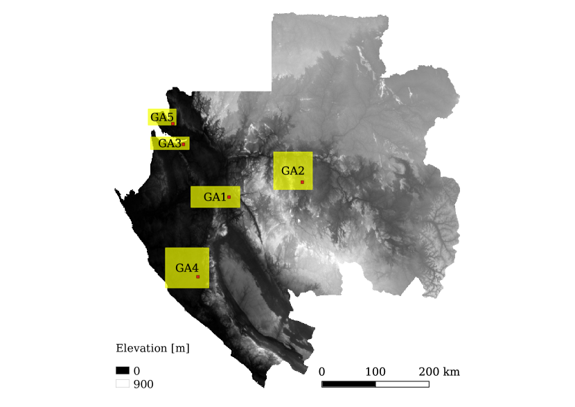
In February/March 2016 NASA’s airborne Land, Vegetation, and Ice Sensor (LVIS) captured full waveform LiDAR scans in five regions in Gabon, see Figure 1. The measurement campaign covers mangrove forests with a maximum height of 71.1 m in the Pongara National Park (GA3) and tropical forests with canopy heights up to $>$85 m in the Lope National Park (GA2). With a nominal flight altitude of 7300 m the LiDAR beams have a footprint of 18 m, with along-track and across-track spacing of $\approx$10 m. The LVIS data is available in two products [Blair and Hofton, 2018]. The Level 1B product contains geolocated laser return waveforms and the Level 2 product height metrics derived from them. We use the geo-referenced canopy top and ground points from the Level 2 product to construct the ground truth canopy height model (CHM) with 10 m GSD. In the resulting CHM we bi-linearly interpolate missing heights that are completely surrounded by valid canopy height values to obtain a dense ground truth map. We regard the heights derived from full-waveform LiDAR as ground truth, with for our purpose negligible errors. Note, combining training data from several different, sizeable areas (in total more than 2000 km²), and recorded during five different flights, greatly reduces the risk of systematic errors from individual measurement campaigns.

Figure 2: Switzerland ground truth: Canopy height vs. slope visualised as 2D histogram.

3.3 Switzerland / Alps

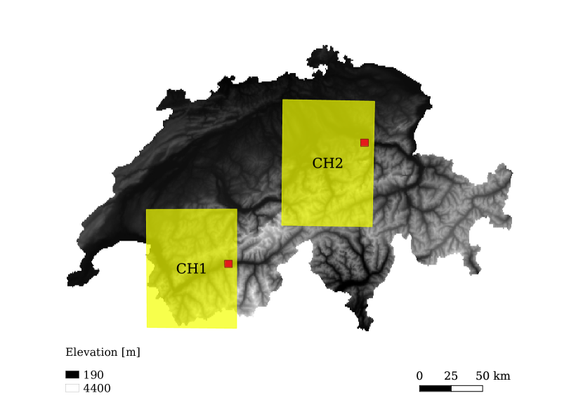
The Swiss Federal Institute for Forest, Snow and Landscape (abbreviation: WSL) created a digital surface model (DSM) by photogrammetric stereo matching [Ginzler and Hobi, 2015], based on aerial imagery acquired by the Federal Office of Topography (swisstopo). The resulting DSM was then converted to a canopy height model by subtracting an existing digital terrain model (DTM) and masking out the buildings. The original CHM has 1 m GSD, we reproject it to UTM WGS84 and resample it to the 10 m GSD of Sentinel-2. The base imagery is acquired in a continuous, cyclic scheme in a way that all of Switzerland is covered in leaf-on conditions (May–September) over a period of six years. We use two regions updated in 2016, the same year for which we collect the satellite images over Switzerland. These regions contain parts of the Swiss Plateau, the Pre-Alps, and the Alps, with an altitude range of 190 to 4400 m and a variety of forest types [Ginzler and Hobi, 2015].

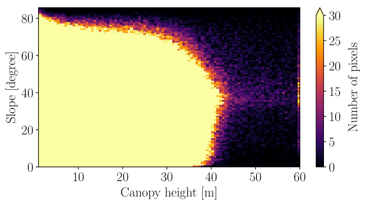
The accuracy of the CHM (in forest areas, after filtering out outliers) was assessed using terrestrial measurements and achieved a RMSE between 3.6 m and 5.0 m. The evaluation indicates that the canopy height errors correlate with slope angle. In some (small) regions with steep terrain, errors in the DSM and DTM – probably residual mis-registration, perhaps also slope-dependent biases – cause grossly wrong canopy heights. Some samples reach up to 60 m, while values $>$40 m are unrealistic for the observed alpine forests. Figure 2 shows the distribution of canopy heights against the slope, where canopy heights $>$40 m occur systematically on steep slopes $>$30^∘. Since these samples account only for a tiny portion of the data (0.03% in region CH1, 0.08% in region CH2), we simply discard them from the test set and validate the performance only on samples with reference height $<$40 m. We note that (both positive and negative) biases of the ground truth due to mis-registration can of course also occur at lower canopy heights $<$40 m. The (small) influence of such cases is ignored.

4 Method

Figure 3: Method overview: A single Sentinel-2 image with 13 spectral bands is used as input (left) to predict canopy height at 10 m GSD. The entry block of our proposed CNN gradually increases the channel depth up to 728 channels using pointwise convolutions. The 18 identical separable convolution (SepConv) blocks do not only learn spectral features that correlate with canopy height, but also spatial context and texture features.

Figure 4: Illustration of the depthwise separable convolution layer [adapted from Bendersky, 2018]. First, separate 2D-kernels are learned for the input layers, each producing its own activation map. Second, these activation maps are combined by applying $1\times 1$ kernels.

4.1 Preprocessing

ESA’s sen2cor toolbox provides standard algorithms to correct atmospheric effects [Mueller-Wilm, 2018]. As a best practice, we use this toolbox for radiometric correction and create the Level 2A product, i.e., bottom-of-atmosphere reflectance. By decreasing variability due to atmospheric effects, the distribution of the image values is homogenised across different sensing dates and geographic regions, which simplifies the regression problem and may lead to improved generalisation. Moreover, the Level 2A product provides also a cloud probability mask, and a pixel-level land cover classification. After atmospheric correction, the lower-resolution bands (20 m and 60 m) are bi-linearly upsampled to 10 m, to obtain a 13-channel data cube with 10 m GSD.

As a final preprocessing step we normalise each channel separately to have mean 0 and standard deviation 1 (across the entire training set), so as to match the requirements of the subsequent model fitting stage. On the one hand, random initialisation then leads to neural network weights of appropriate magnitude for all channels, which speeds up convergence of the training. On the other hand, transforming all feature channels to the same magnitude ensure that parameter regularisation affects them equally. The per-channel means and standard deviations of the training set are stored and, at inference time, used to shift and scale the test data in the same way.

4.2 Deep regression network

Convolutional neural networks (CNNs) are the state-of-the-art technology for many image interpretation tasks, due to their ability to learn multi-scale feature encodings with excellent predictive power from data. Here, we employ them for canopy height estimation from multi-spectral Sentinel-2 images. The principle of CNNs is to extract image features by convolving the input with a set of linear filter kernels, followed by a point-wise non-linear activation function, to obtain so-called activation maps. Stacking that operation, i.e., using the activation maps as input for another layer of convolutions with subsequent activation functions, yields a deep network that gradually transforms the inputs to the desired output values via a sequence of increasingly discriminative representations. The parameters of the filter kernels (also called weights) are learned directly from the data in a supervised fashion.

Our proposed network is adapted from the Xception architecture [Chollet, 2017], see Figure 3. It consists of an entry block followed by 18 identical separable convolution (SepConv) blocks. Activation functions are always rectified linear units (ReLU) that leave positive values unchanged and clip negative values, formally $x_{\text{out}}=\max(0,x_{\text{in}})$. All blocks are residual blocks, i.e., their input is also passed on through a skip connection that bypasses the block and is added to the output activation map, so that the overall block learns an additive residual function to the identity mapping. Skip connections facilitate the learning of very deep networks by creating shortcuts and thus preventing error gradients from vanishing before they reach the early layers. The entry block, inspired by He et al. [2016], consists of three pointwise convolution layers that gradually increase the channel depth of the data cube to 728 channels. I.e., the filter kernels are of size $1\times 1\times d_{\text{in}}$ and together form a non-linear per-pixel mapping to 728-dimensional spectral feature vectors. Since the entry block changes the channel depth, the identity mapping in the skip connection must be replaced by a single linear convolution layer (also with learned weights) that increases the depth from 13 to 728.

The structurally identical SepConv blocks that make up the remainder of the network each consist of two depthwise separable convolutional (SepConv) layers and an identity residual connection that bypasses both. A SepConv starts with the ReLU non-linearity. Then follows a depthwise separable convolution layer (Figure 4). In that layer, the overall 2D-convolution with a 3D-kernel is factored into 2D-kernels (in our case, $3\times 3$) applied to each input channel, and a 1D-kernel (linear combination) that combines the results from all channels. The factorisation decouples spatial and across-channel correlations, thereby reducing the number of parameters to be learned. The number of parameters is reduced by reusing the activation maps of the spatial kernels ($3\times 3$) as input to all subsequent point-wise kernels – in our case by a factor of $\approx$9. After the separable convolution follows a batch normalisation (BatchNorm), which renormalises the data cube for a batch (training examples are passed through the network in small batches, see below). The repeated re-normalisation reduces the sensitivity of the network to the initialisation and allows for much higher learning rates during gradient descent [Ioffe and Szegedy, 2015]. Moreover in conjunction with the ReLU activation it amplifies the non-linearity, by ensuring the presence of negative activations.

After 18 SepConv blocks the final layer of our network is a pointwise convolution that combines the 728 activation maps into a single canopy height value per pixel. Overall, the network has 19,604,225 trainable weights. Since we are facing a regression problem with continuous (height) values as targets, we learn those parameters by minimising the $\ell_{2}$-loss, i.e., the mean square error over the training examples. Furthermore, we include an optional $\ell_{2}$-penalty on the parameters (“weight decay”) to regularise the fit, such that the total loss function we minimise is

$$Loss=\frac{1}{N}\sum_{i=1}^{N}\left(f(x_{i})-y_{i}\right)^{2}+\lambda\frac{1}{W}\sum_{j=1}^{W}\left(w_{j}\right)^{2}$$ (1)

, with the model $f$ and its weights $w_{i}$ (including the constant biases per kernel), input intensities $x_{i}$, ground truth canopy heights $y_{i}$, and the prediction $f(x_{i})$ at pixel $i$. $N$ and $W$ denote the numbers of samples and weights, respectively. The hyperparameter $\lambda$ controls the strength of the regularization. We note that, in contrast to a number of CNN architectures popular in generic computer vision, we deliberately do not down- or up-sample the activation maps at any point. There is no max-pooling and all convolutions are computed with stride 1. The data cube is padded at its borders before every 3$\times$3 convolution, to maintain the size of the input.

4.3 Model learning

We use a patchwise training procedure with patches of size $15\times 15$ pixels, corresponding to $150\times 150$ m² on the ground. These patches are sampled randomly from all valid ground truth locations in the training areas, consequently each patch has at least one valid ground truth pixel at its center. Pixels with missing ground truth do not contribute to the per-patch loss, such that they do not affect the training procedure. At training time we used the Level 2A cloud probability mask to exclude cloudy patches: pixels with $>$10% cloud probability are considered as cloudy, and any patch with $\geq 10$% cloudy pixels is discarded. With this procedure we avoid showing the network confusing patches with too little signal, but enable it to learn textural features that are robust near the cloud borders.

The optimisation of the parameters in deep networks is done by mini-batch stochastic gradient descent (SGD). To that end, one applies the network to a (small) subset of training samples, which is called forward pass, and from the response computes an approximation to the gradient (partial derivative) of the loss function w.r.t. every network weight. As the CNN constitutes a nested sequence of transformations, those derivatives can be computed with the chain rule and back-propagated through the network, traversing it from the output to the input. The training procedure consists of iteratively drawing batches of training samples, back-propagating the error gradients, and updating the weights with small steps in the negative gradient direction. The step size is controlled by scaling the gradients with a hyper-parameter called the learning rate. We use a popular variant of SGD called ADAM [Kingma and Ba, 2014] that adaptively adjusts the learning rate for each trainable parameter by normalizing the global learning rate with the running average of the gradient. This has the effect of amplifying the step size along low gradients and attenuating it for high gradients. In this way, the solver is less sensitive to the chosen base learning rate, and there is no need to design a careful learning schedule.

For the experimental evaluation of our method the base learning rate is set to 0.0001 and the batch size to 36 patches, dictated by memory constraints of the GPU hardware (in our case an Nvidia GTX 1080 with 8 GB memory). I.e., during a complete training run of $\approx$50,000 iterations the network sees about 1.8 million randomly sampled patches.

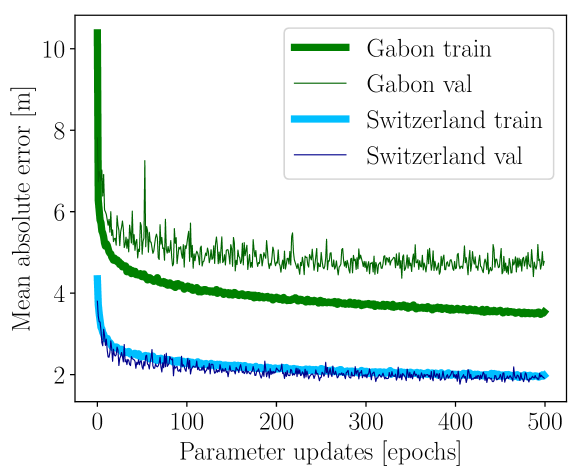
The available data is first split into two geographically separated parts, a training set and a test set that is never seen during training and only used to evaluate the performance of the trained model. The training set is, in turn, split into a training part and a (smaller) validation part, where the latter is never used to compute gradients for back-propagation. The learning process is monitored by observing both the training loss and the validation loss. The former indicates how well the model fits the training data, whereas the latter is an estimate of how well the model generalises to unseen data. Stagnation of the validation loss is a sign that the training has converged and further iterations may cause overfitting of the training data. We keep training until the loss on the training set has converged, which takes $\approx$50,000 iterations for a single training region, and $\approx$250,000 iterations when training a single model across all regions. Following standard practice, we regularly (in our case every 500 iterations) calculate also the loss on the validation set. Figure 5 depicts the two loss curves over the training iterations. As our final set of model parameters we pick those that achieved the lowest validation loss.

Figure 5: Loss curves for the training and validation data in Gabon and Switzerland. One epoch corresponds to 500 training iterations.

4.4 Evaluation

The performance of the trained model is then evaluated on the unseen test region, by measuring the mean absolute error (MAE),

$$MAE=\frac{1}{N}\sum_{i=1}^{N}\left|f(x_{i})-y_{i}\right|\;$$ (2)

and the root mean square error (RMSE),

$$RMSE=\sqrt{\frac{1}{N}\sum_{i=1}^{N}\Big{(}f(x_{i})-y_{i}\Big{)}^{2}}\;.$$ (3)

Our proposed architecture is fully convolutional, meaning that all layers can be applied to input images of arbitrary size, within hardware memory limits. To generate large-scale maps, test images are cut into tiles of $128\times 128$ pixels, with 8 pixels overlap to mitigate tiling artifacts. We run inference on all tiles, recompose them into a map, then mask pixels with cloud probability $>10$%. Moreover, water pixels according to the Level 2A land-cover classification are excluded from the quantitative evaluation to avoid over-optimistic results: water has a rather distinctive spectral signature and correctly predicting 0 m canopy height over water bodies is fairly trivial. In Switzerland we also exclude pixels classified as snow, because snow strongly alters the spectral signatures.While we do not exclude the possibility that vegetation height could also be estimated from data with some degree of snow cover, this would likely require a separate, dedicated model.

5 Results and discussion

We quantitatively evaluate our approach on 7 regions in total, 5 in Gabon (GA) and 2 in Switzerland (CH). See Figure 1. Each region is split into spatially disjoint training, validation, and test sets. Depending on the region, four to twelve Sentinel-2 images are available that have overall cloud coverage $<$70% (Table 1). The CNN is trained on images from multiple acquisition dates, assuming that the vegetation height did not change significantly within the investigated time interval. This makes the CNN more robust against radiometric variations due to remaining atmospheric effects, illumination, vegetation activity, or water content. In the test set, we predict high-resolution vegetation height maps individually for each date, and merge the resulting stack of predictions. This greatly reduces gaps due to clouds. We have tested two simple merging strategies, choosing the median height and selecting for each pixel the prediction with the lowest cloud probability (minCloud). The median, which benefits from the redundancy of multiple predictions and is less affected by inaccuracies of atmospheric correction and cloud masking, works slightly better; reaching MAE of 4.3 m for Gabon and 1.7 m for Switzerland. The RMSE is more sensitive to rare, large deviations and achieves 5.6 m and 3.4 m for Gabon and Switzerland, respectively. See Table 2. Given the tight correlation between the two metrics, we only show the MAE for further analyses. We point out that even the minCloud strategy, which effectively is based on a single “best” spectral signature per pixel without any temporal redundancy, achieves decent results of 4.9 m, respectively 2.0m; indicating that, if need be, one can retrieve reasonable vegetation heights from a single cloud-free view. Furthermore, the spread between individual per-image estimates from different days of the year is only a fraction of the MAE: their standard deviation lies between 0.1 m and 0.2 m for Switzerland, and between 0.3 m and 0.6 m for Gabon. See Figure 9. Unless explicitly stated, the reported results in the remainder of this section are median values over all cloud-free dates. It should be noted in this context that the multi-temporal co-registration accuracy of Sentinel-2 is $\approx$12m [Clerc and MPC Team, 2019], corresponding to 1.2 pixels at 10 m GSD. Consequently, computing the median across time likely induces a mild spatial smoothing of the canopy height maps.

We evaluate the generalisation across sensing dates and across geographical regions within Gabon and Switzerland, respectively. Furthermore, an ablation study is conducted to assess the importance of different spectral bands for canopy height estimation. Finally, we also empirically test the influence of spatial texture patterns, by disabling the ability of our model to exploit spatial context.

Ablation studies are carried out on the two regions GA3 and CH2, which are the most suitable representatives of their respective geographic regions. Both span the whole range of canopy heights and have a moderate cloud-cover so that generalisation across time could be tested. In experiments that use only a single region for training we empirically set the regularisation of the model parameters to $\lambda=0.001$. When training on (more and more diverse) data from across the country, the best results were achieved without regularisation, $\lambda=0.0$.

ROI name	Images	train [px]	val [px]	test [px]
GA1	6	4822K	647K	1124K
GA2	7	5826K	955K	1575K
GA3	4	4393K	1012K	1008K
GA4	5	3674K	964K	1077K
GA5	4	2171K	498K	490K
CH1	8	31913K	7499K	9681K
CH2	12	26947K	6701K	8461K

Table 1: Test regions with available ground truth data.

Figure 6: Example images for the test area in GA1, showing strong cloud coverage.

5.1 Results for reference areas

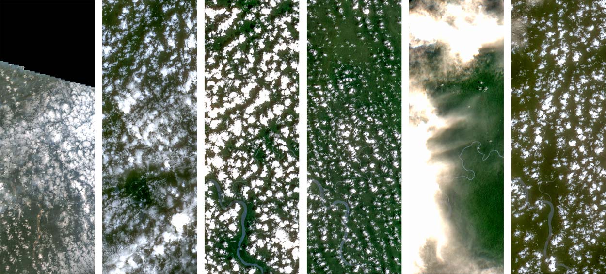
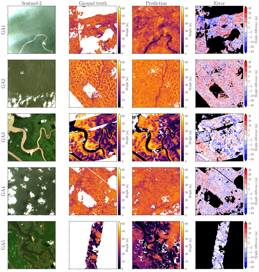
In Table 2 we show the retrieval accuracy for each of the seven regions, as well as the overall performance per country. The CNN trained jointly on the five different training areas in Gabon yields predictions with MAE 4.3 m across all test regions in Gabon. The test area with the lowest error is Pongara National Park (GA3), an area of mangrove forest, where the MAE is 3.7 m, despite being based on only four sensing dates, due to frequent cloud cover. In line with previous results, the predictions have higher error in dense and high forest. In Lope National park (GA2) the MAE is 4.6 m. The worst result is 5.2 m MAE for region GA1, presumably due to the influence of cloud shadows (Figure 6).

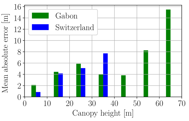
When fitting to both training areas in Switzerland, the predictions across both test areas have a much lower MAE of 1.7 m. This confirms the general trend that prediction is easier for lower vegetation height and density. Accordingly, for CH1 with on average lower canopy height we obtain MAE 1.5 m, whereas the higher CH2 has MAE 2.0 m. A more detailed view of the prediction performance in different (ground truth) height classes is given in Figure 7. Switzerland exhibits a roughly linear correlation between height and MAE, where the relative prediction error is about 20% across all heights. In Gabon the general behaviour is similar, but we observe significantly better relative accuracy in the range of 30-55 m.

Figure 7: Mean absolute errors per 10 m canopy height intervals.

(a) Gabon

(b) Switzerland

Figure 8: Confusion plots for Gabon and Switzerland: Ground truth vs. prediction visualised as 2D-histograms with 1 m bins.

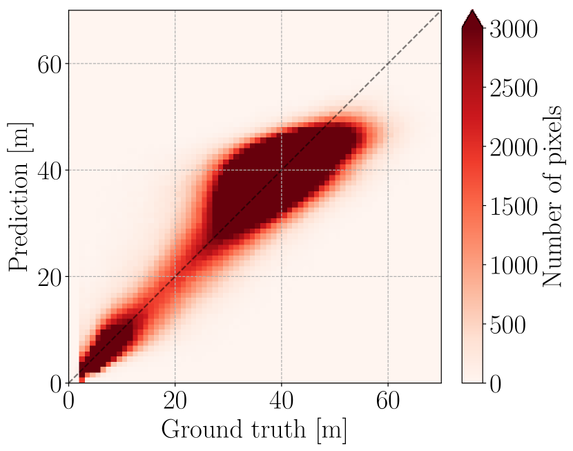
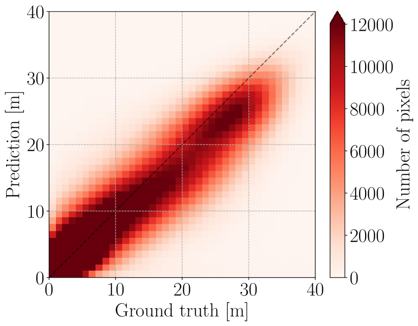
The scatter plots in Figure 8 show good agreement between predictions and ground truth heights. One can see that, in Gabon, there is a slight trend to overestimate canopy heights around 30 m. A closer inspection reveals that this happens mainly in regions densely covered by high forest, where those 30 m represent the lowest observed values. Moreover, the model does not predict values above $\approx$55 m and therefore underestimates very high vegetation in the range 50-70 m. This effect in high and dense forest is in line with previous results, it appears that the canopy reflectance of rainforest saturates at a certain height and then no longer changes [Hansen et al., 2016, Simard et al., 2011]. We find that also the textural information is not discriminative above that height, which is perhaps not surprising, because the species composition as well as the shape of individual tree crowns do not vary a lot above 50 m. In Switzerland, the predictions in general follow the ground truth more closely. Also here, underestimation occurs for high vegetation. Interestingly, we see an almost constant offset of about -2.5 m for canopy height $>$15 m. Furthermore, underestimation of low vegetation heights $<$5 m is more frequent. In part this is probably simply a consequence of the large proportion of samples at that height. We note, though, that a part of the error may be due to the reference data, since photogrammetric surface reconstruction is less reliable on low and sparse vegetation. Also temporal changes due to agricultural plants might play a small role (e.g., corn grows to $>$2 m).

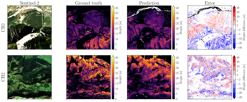
Example results are depicted in Figures 10 and 11. Each row corresponds to a different region, showing a 5$\times$5 km² sub-sample from the test set. The spatial distribution of the vegetation height is recovered well, also large local variations in vegetation height are resolved correctly (such as in region GA3). Even fine canopy structures with extents $<$100 m are captured, but they tend to be over-smoothed (for instance in GA2). I.e., while very high trees $>$50 m are under-estimated (as discussed above), lower ones near them tend to be over-estimated. This effect seems to be a main reason for the over-estimation of canopy heights around 30 m (see scatter plot in Figure 8), as that is the typical height of the lower vegetation occurring near very high stands.

Name	All minCloud		All median		W/O median
	mae	rmse	mae	rmse	mae	rmse
GA1	5.7	7.3	5.2	6.7	5.7	7.3
GA2	5.4	6.9	4.6	5.9	6.9	8.6
GA3	4.1	5.6	3.7	5.1	6.9	9.3
GA4	4.5	5.8	4.1	5.3	4.7	6.0
GA5	4.2	5.7	4.0	5.3	4.1	5.5
CH1	1.6	3.3	1.5	3.0	1.9	3.7
CH2	2.4	4.5	2.0	3.8	2.2	4.1
GA all	4.9	6.5	4.3	5.6	6.0	7.9
CH all	2.0	3.9	1.7	3.4	2.1	3.9

Table 2: Fusion strategies, and generalisation across different geographic regions in a country. The table compares MAE and RMSE (in meters) for: (i) Merging multi-temporal predictions with the median vs. the minCloud strategy (1${}^{\text{st}}$ and 2${}^{\text{nd}}$ column). (ii) Training on training areas of all regions in a country vs. training only on training areas of the 4, respectively 1, other regions (W/O), without seeing data from the immediately adjacent training area (2${}^{\text{nd}}$ and 3${}^{\text{rd}}$ column).

Figure 9: MAEs of individual per-image predictions (grey) with the average MAE and standard deviation (error bar).

Figure 10: Qualitative results for Gabon: Rows show 5$\times$5 km² sub-samples (10 m GSD) from the test areas of the five regions (GA1-5). From left to right the columns show the clearest Sentinel-2 image, the ground truth canopy height, the prediction of our model, and the error (prediction minus ground truth). Positive errors (red) occur when the prediction is higher than the ground truth. No data is displayed in white or black, respectively.

In Switzerland (Figure 11) the absolute error for zero canopy height is $<$1 m, i.e., the model has implicitly learned to recognise the absence of trees and bushes. Moreover, low forest (10-20 m) tends to be underestimated, such as in CH1. One specific problem in Switzerland are outliers in the reference data used as ground truth. On very steep slopes the reference data contains narrow strips of implausible heights up to 60 m. These are likely due to the way the CHM has been generated, by subtracting a reference bare-earth DEM from a surface model. Mis-registration or systematic errors on steep slopes can then cause large differences, even in the absence of any high vegetation. Figure 12 shows an example of such a situation, where the ground truth CHM contains values up to 60 m, whereas our model predicts canopy height 0 m, consistent with a visual inspection of the images. As explained above, we therefore remove the tiny portion of samples $>$40 m from the test set. We did not find it necessary to remove the incorrect pixels from the training set, as the training is apparently robust against them and the model never predicts heights $>$40 m. Overall, the prediction errors for Switzerland are in the same range as the 3.3 to 5.5 m uncertainty of the canopy height model that we use as ground truth, according to Ginzler and Hobi [2015]. We believe that complementary observations (e.g., airborne LiDAR) or extensive field work would be necessary to disentangle biases of the model from biases in the training data as well as the reference data.

Figure 11: Qualitative results for Switzerland: Rows show 5$\times$5 km² sub-samples (10 m GSD) from the test areas of the two regions (CH1/2). From left to right the columns show the clearest Sentinel-2 image, the ground truth canopy height, the prediction of our model, and the error (prediction minus ground truth). Positive errors (red) occur when the prediction is higher than the ground truth. No data is displayed in white or black, respectively.

In both geographic regions we observe some degree of over-smoothing. This is a price to pay for using CNNs and modelling texture context, as information is accumulated and mixed over larger receptive fields. It may be possible to mitigate the smoothing by using different loss functions. The $\ell_{2}$-penalty (mean square error) used here is known to be biased towards smooth outputs without height discontinuities. E.g., an $\ell_{1}$-penalty (mean absolute error) would instead induce a bias towards piecewise constant heights with bigger jumps. Further investigations in this direction are left for future work.

Figure 12: Illustration of DEM errors in Swiss CHM. The blue box in the first image marks a 1$\times$1 km² example area with steep slopes, magnified in the remaining columns.

5.2 Generalisation across time and space

Name overall 0-10 [m] 10-20 [m] 20-30 [m] 30-40 [m] 40-50 [m] 50-60 [m] 60-70 [m] GA3 5.7 (0.7) 3.5 (1.4) 5.8 (1.6) 6.7 (1.3) 6.5 (0.6) 7.2 (2.0) 9.8 (2.1) 13.8 (2.4) CH2 2.8 (0.3) 1.4 (0.3) 5.3 (0.6) 5.8 (1.3) 8.3 (2.0) - - -

Table 3: MAE with cross-validation over sensing dates. Numbers in parenthesis are empirical standard deviations. Compare to 2${}^{\text{nd}}$ column of Table 2.

To analyse our model’s ability to generalise to new sensing dates, we perform leave-one-out cross-validation across different dates (respectively, satellite passes), for the regions GA3 and CH2. All retrieved acquisition dates in our considered time period except one are used for training, the remaining one for testing. This leads to 4-fold cross-validation for GA3, respectively 12-fold cross-validation for CH2. In Table 3 we report the average MAE over all folds, together with its empirical standard deviation. The baseline performance with all dates is given in Tables 4 and 5. For the Gabon site we obtain a MAE of 5.7$\pm$0.7 m, compared to 3.7 m when training on all dates. For the Swiss site the MAE is 2.8$\pm$0.3 m, compared to 2.6 m with all dates. Note, the experiment is not able to separate the impact of simply having less, and less varied, training data from the influence of not having trained on the exact same imaging conditions. Both effects should, according to conventional wisdom, diminish as larger training sets with greater diversity are used.

The generalisation across geographical regions (that share reasonably similar climate and biome) was tested by leave-one-out cross-validation between the regions of the respective country. I.e., we train on the training areas of all but one region in Gabon (respectively, Switzerland) and test on the test area of the remaining region, such that no training data from near the test area is seen during training; resulting in 5-fold, respectively 2-fold cross-validation. The outcomes of that test are summarised in Table 2. As expected from Tobler’s First Law of Geography, the performance drops a bit for all regions, as the domain gap between training and test data increases with growing distance. The largest drops are observed for Lope National Park (GA2) from 4.6 m to 6.9 m and for Pongara National Park (GA3) from 3.7 m to 6.9 m. While again the larger MAE is a combination of seeing less data and seeing less representative data, in these cases the latter effect is very likely the dominant cause, as these two regions exhibit rather unique vegetation characteristics not present in the remaining regions. GA2, in particular, has very high vegetation with average height $>$40 m in the test area, a situation which the model is not exposed to when training on the remaining regions. The assertion that each of those two regions has a significant domain gap to all others is supported by the fact that for the other three regions in Gabon performance drops only by 0.1 to 0.6 m.

For Switzerland the performance when training on one region and testing on the other only decreases by 0.4 m, respectively 0.2 m. Since we only have data from two distinct regions of similar size, but fairly similar vegetation type, that drop is probably mostly caused by the lower amount of training data (roughly half).

5.3 Ablation study: spectral bands

To gain some insight into the importance of different spectral bands of Sentinel-2 for vegetation height mapping, we train and test with several different band combinations. The following subsets of bands have been evaluated, by simply changing the spectral channel depth of the input and retraining, leaving all other specifications of the CNN unchanged. RGB: the visible bands with 10 m GSD (B02, B03, B04); N: only the 10 m NIR band (B08); RGBN: all four 10 m bands; woRGBN: all 20 m and 60 m bands (B01,B05-07,B08a-12); ALL: all 13 bands. In Tables 4 and 5 the results are shown for the regions GA3 and CH2. For both regions the performance of ALL and RGBN are similar, indicating that the high-resolution bands carry most of the relevant information, whereas the other nine bands (upsampled to 10 m GSD) contribute only little. A tentative common pattern is that towards the top of the height range the 20 m and 60 m bands seem to rather deteriorate than improve the regression. This would be consistent with the observation that for high trees texture features are more beneficial (see below). But further investigations with more geographic diversity are needed to confirm that trend. In Gabon, only RGBN also achieves markedly lower MAE for very low vegetation. Further research is needed to understand why, one may speculate that it has to do with the implicit spatial smoothing of the spectral information when upsampling low-resolution bands to 10 m. All other band selections perform significantly worse in Gabon.

In Switzerland one even obtains a slight improvement when using only RGBN instead of ALL channels – again it is not statistically meaningful to assess the significance of that result based on one test region, and further tests are needed. Contrary to Gabon, even using only the visible RGB works rather well. Whereas the perhaps clearest message of the study is that using only near-infrared is not sufficient.

Name overall 0-10 [m] 10-20 [m] 20-30 [m] 30-40 [m] 40-50 [m] 50-60 [m] 60-70 [m] ALL 3.7 2.6 3.7 4.4 3.8 4.5 5.9 7.5 RGB 5.0 2.7 5.4 6.9 5.9 5.1 7.2 10.3 N 6.0 2.7 5.4 8.1 7.6 8.7 8.3 8.6 RGBN 3.8 1.8 3.4 5.1 4.8 5.3 5.8 6.9 woRGBN 4.8 2.0 4.7 5.8 5.2 7.6 11.2 14.5 ALL 1$\times$1 6.0 1.8 5.1 7.7 6.6 11.3 17.1 22.0

Table 4: Ablation study Gabon (GA3): MAE for various band selections, and for strictly pixel-wise spectral features (ALL 1$\times$1).

Name overall 0-10 [m] 10-20 [m] 20-30 [m] 30-40 [m] ALL 2.6 0.9 4.4 6.0 8.6 RGB 2.5 1.3 4.4 5.1 8.8 N 3.3 2.0 6.0 6.0 8.3 RGBN 2.2 1.1 4.5 4.9 7.1 woRGBN 2.7 1.2 4.9 6.3 9.9 ALL 1$\times$1 3.6 2.2 4.4 6.8 12.8

Table 5: Ablation study Switzerland (CH2): MAE for various band selections, and for strictly pixel-wise spectral features (ALL 1$\times$1).

(a)

(b)

(c)

(d)

Figure 13: Activation maps of selected $3\times 3$ filter kernels our model learns. Left corresponds to shallower, right to deeper network layers. White means low activation, red/blue are strong positive/negative responses. One can see sensitivity to vertical and horizontal edges (a,b), water (c) and high vegetation (d).

5.4 Influence of texture features

One reason for using a CNN as regressor has been our assumption that at resolutions as high as the 10 m of Sentinel-2, where single trees can be as big as the pixel footprint, textural features may play an important role. By stacking many convolutional layers with 3$\times$3 filter kernels, our network learns to pick up texture patterns in a larger receptive field centred at each pixel, if they correlate with vegetation height. To check whether this is indeed necessary, we restrict the network to look only at the spectral distribution of each individual pixel, by setting the spatial size of all convolution kernels to $1\times 1$. This prevents it from seeing any texture or spatial context. Otherwise the CNN architecture (number of layers, channel depth per layer) is the same, so that the restricted network derives its prediction at a given pixel only from that pixel’s spectral intensities, but still allows for the same degree of non-linearity in the mapping. The results are also reported in Tables 4 and 5, denoted as ALL 1$\times$1. For GA3 the MAE grows from 3.7 m to 6.0 m, for CH2 it increases from 2.6 m to 3.6 m. The biggest differences occur in the height range of 40-60 m. This demonstrates the benefit of including texture features when dealing with high-resolution images, especially in areas of very high vegetation. Previous work dealing with vegetation height and structure [e.g., Ota et al., 2014, Tyukavina et al., 2015, Hansen et al., 2016] has mostly ignored texture. There may indeed not be as much benefit in looking beyond per-pixel signatures when one deals with lower sensor resolutions like the 30  m of Landsat, or even less.

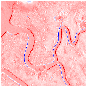
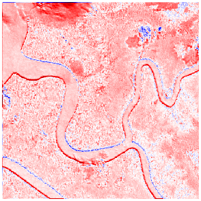
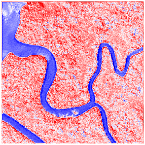
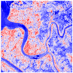
In Figure 13 we illustrate a few of the learned texture features that have a clear interpretation. We show the activation maps after applying the respective convolution kernel. Filters in early layers extract low-level primitives such as vertical and horizontal contrast edges. Deeper layers combine those lower-level activations over larger receptive fields into more task-specific features that fire, for instance, on high vegetation or on water.

An open question in this context is whether spatial textures should be used in conjunction with longer time series and more sophisticated multi-temporal representations than our simple median, to further improve the predictions. The fact that we can get very reasonable predictions even from single images could also indicate that texture might, to some degree, be able to compensate for temporal redundancy and vice versa.

5.5 Large-scale canopy height maps

(a) Our map for 2017 (10 m GSD)

(b) NASA map for 2005 (1 km GSD)

(c) WHRC map (30 m GSD)

Figure 14: Our country wide vegetation height map of Gabon (top row) compared to existing maps from NASA [Simard et al., 2011, bottom left] and WHRC [WHRC, 2015, bottom right]. The latter is only available as RGB colour image, hence we depict it with the original colour map. Note that the height saturates at 15 m.

(a) Our map for 2017 (10 m GSD)

(b) WSL map 2007-2016 (10 m GSD)

(c) NASA map for 2005 (1 km GSD)

Figure 15: Our country wide vegetation height map of Switzerland (top) compared to existing maps from WSL [Ginzler and Hobi, 2015, bottom left] and NASA [Simard et al., 2011, bottom right].

Figure 16: Cumulative distribution of country-wide canopy height predictions.

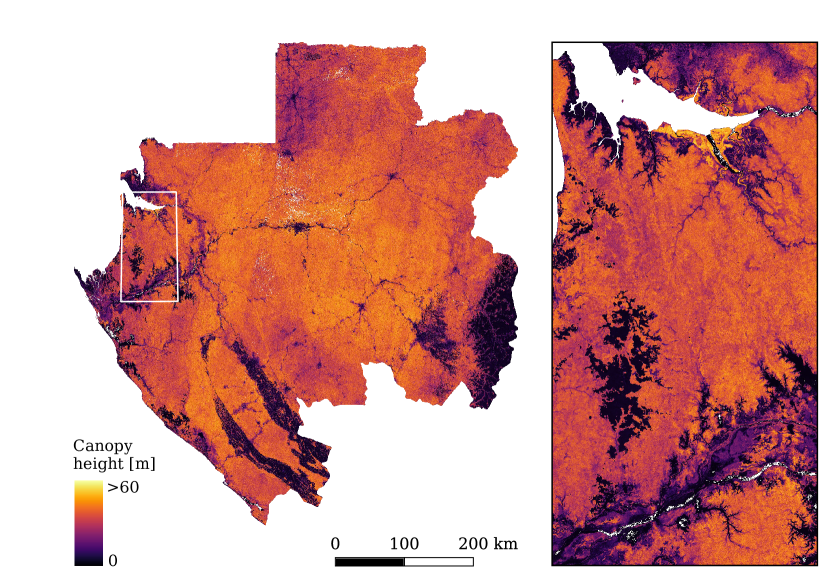
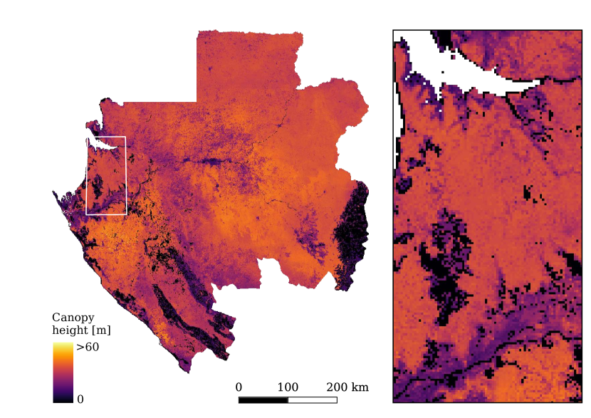
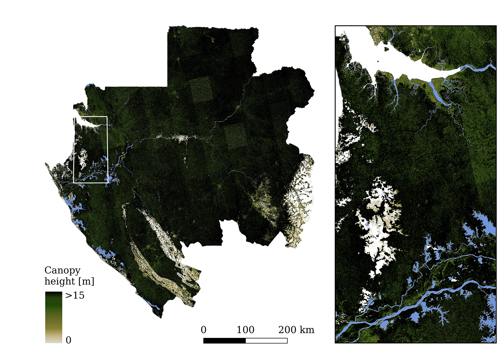
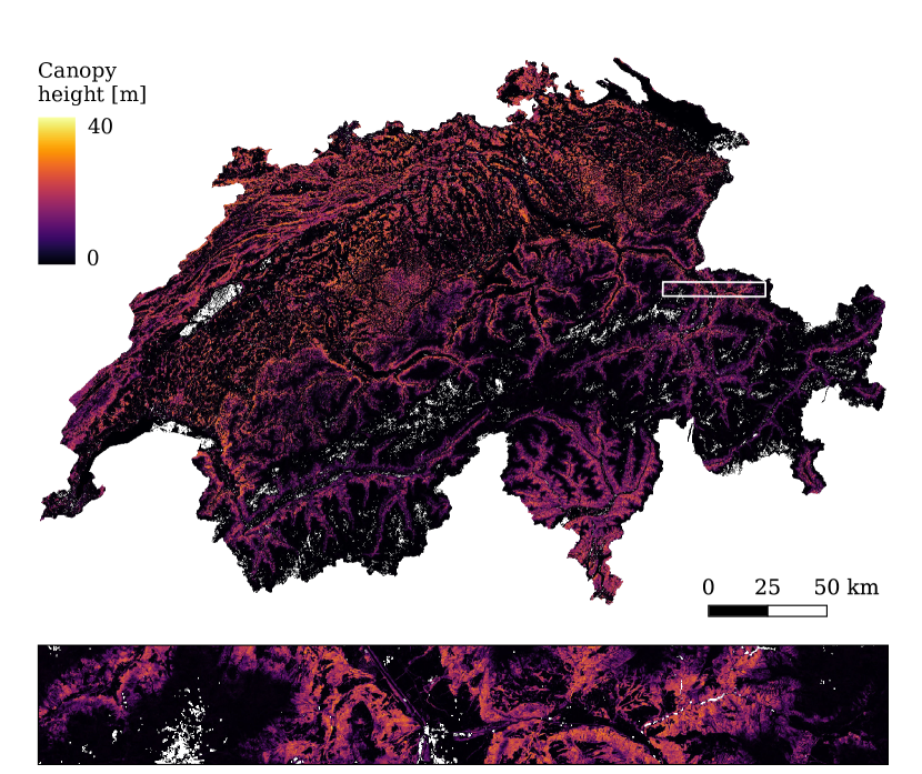
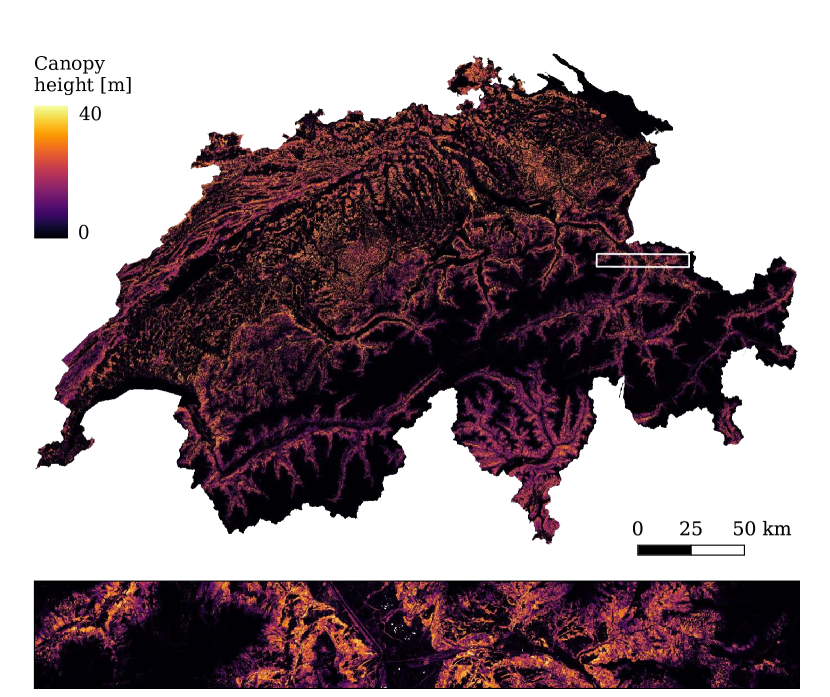
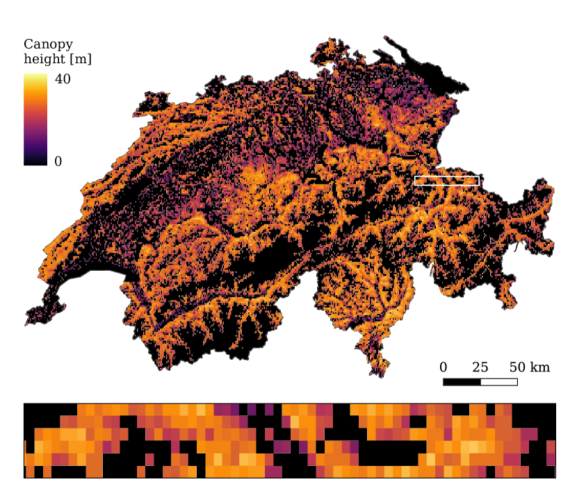
We have also computed country-wide canopy height maps at 10 m resolution for Gabon (Figure 14) and Switzerland (Figure 15). Sentinel-2 images are organised in 100$\times$100 km² tiles, such that 56,984 tiles cover the globe.

Hence, 47 tiles are needed to cover Gabon, 13 are needed for Switzerland. To ensure cloud-free coverage of (almost) the entire country, we automatically pick, for every tile, the 10 dates within 2017 (May–September for Switzerland) that have the lowest cloud coverage, predict canopy heights for all cloud-free pixels, and take the median over the cloud-free predictions at each pixel.

We qualitatively compare the resulting vegetation height maps to existing maps from NASA [Simard et al., 2011, both locations], WHRC [WHRC, 2015, Gabon; map available only for the tropics], and WSL [Ginzler and Hobi, 2015, map produced locally for Switzerland]. Temporal offsets are inevitable: our maps represent the state in 2017. The others mix inputs over longer time periods, due to the recording schedules of the underlying image and/or reference data. Both, the NASA map and the WHRC map are fitted to ICESat GLAS LiDAR heights. While Simard et al. [2011] used global high-level products such as tree cover, elevation, and climatology to interpolate the LiDAR samples to a global 1 km grid, WHRC [2015] fit a regression from ALOS PALSAR to the LiDAR heights, with 30 m GSD. For the WSL map [Ginzler and Hobi, 2015] DSMs were generated with airborne photogrammetry and reduced to vegetation heights with an existing country-wide bare-earth DTM. The original data has nominal GSD 1 m, we downsampled it to 10 m for a direct comparison.

For Gabon, we find that the large-scale structures are in good agreement between all three maps. The NASA map tends to miss small structures due to its coarser resolution. While this is not an issue for large-scale studies, e.g., of the global climate; detailed information is important for local decisions, such as the protection of high forest near settlements, as recommended by the High Carbon Stock (HCS) approach. Moreover, in the NASA map very high regions, like the Mangrove forest in Pongara National Park near the top of the zoomed region, are missed. Also the somewhat lower heights around central Gabon’s Lope National Park appear implausible, we speculate that the very frequent cloud coverage in that region may have impacted some of the products on which the map is based. In that region our map still has a few missing pixels, which were cloud-covered in all 10 selected images. Further images for that tile need to be processed to fill the gaps. In the north of the country, around the city of Oyem, our model predicts visibly lower heights than NASA. At this point we do not have ground truth to determine which prediction is more correct.

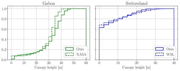
The WHRC map appears to be very accurate in regions of low or missing vegetation, as expected for a RADAR-based estimate. On the contrary, strong under-estimates are observed in wetlands such as Pongara. In general, the low 15 m cut-off is a serious limitation in Gabon, where practically all forest is higher than 30 m, such that the map largely degenerates into a binary forest layer – the overwhelming majority of apparent height structures on closed canopies are in fact noise. According to our prediction (see cumulative distribution in Figure 16) only $\approx$10% of Gabon’s area has vegetation height $<$15 m. More than 60% of Gabon is covered with forest higher than 30 m, and $>$20% are $>$40 m. While the NASA map indicates an average canopy height of 29.6 m, our prediction yields an average of 32.1 m.

For Switzerland, the inter-comparison results look rather different. The WSL map and ours show good agreement. Our result looks a bit smoother, which is likely a result of the implicit smoothing when using large receptive fields. Moreover, like in the quantitative evaluation, our model systematically tends to predict slightly lower values for very high vegetation. The NASA map appears to strongly over-estimate both the vegetated area and the vegetation height throughout Switzerland. The reason for this behaviour is unclear, we speculate that it may partly be due to some uncompensated influence of the steep, mountainous topography on the underlying input products.

In both of our large-scale maps some boundary artifacts remain at the borders of the satellite passes. Bigger overlaps and/or cross-fading between adjacent images may mitigate this effect. Furthermore, it may be beneficial to perform additional radiometric adjustment at the borders of the input tiles.

Processing a 10,000 km² (bottom-of-atmosphere reflectance) tile with our model takes $\approx$35 minutes on one GPU. In total we used 274 GPU-hours for Gabon (470 tiles) and 76 GPU-hours for Switzerland (130 tiles). It has been reported that 94,093 Sentinel-2 tiles are needed to create a cloud-free composite of the global land masses [Kempeneers and Soille, 2017]. From this we can estimate a processing time of a bit over 6 GPU-years for a world-wide map. While this may seem a lot, it is equivalent to 2.3 days on a computing cluster with 1000 GPUs – which nowadays is feasible without major problems.

6 Conclusion

Our proposed data-driven approach allows one to map vegetation height at 10 m resolution. We show that the regression from few Sentinel-2 images achieves low error in the tropics as well as in central Europe, and that our method is suitable for country-scale canopy height mapping in terms of generalisation and computation time. Our CNN-based learning engine, which is able to exploit spatial context and texture features, can predict a high-resolution vegetation height map from a single cloud-free image with good accuracy. Based on these findings, we are convinced that global-scale vegetation height mapping at an unprecedented 10 m resolution can be done operationally, especially in combination with new data sources like the GEDI mission [GEDI Team, 2019]. That resolution would enable a new set of applications requiring localized vegetation structure, e.g., targeted forest protection in the context of the High Carbon Stock approach, or fine-grained biodiversity studies relating vegetation heterogeneity to species richness. Ultimately, retrieval from Sentinel-2 could in some cases reduce the need for expensive LiDAR flight campaigns. Besides the high spatial resolution, Sentinel-2 provides a new image every 5 days, which enables frequent updates, and helps to obtain good coverage even in regions with frequent clouds. That capability, in turn, opens up the possibility to continuously monitor forest degradation and loss around settlements and agricultural lands.

A limitation of our current approach, to be addressed in future work, is its rudimentary use of multi-temporal information. Spectral time series could potentially correlate even better with canopy height. However, we found that satisfactory performance can be reached without relying on long cloud-free time series.

For us, the most important question is: how to extend our method to global coverage? While Sentinel-2 data is globally available, the current models are limited by the available training data and will likely not generalise well to unseen regions of the world. A viable approach, albeit logistically challenging, could be to collect diverse training data for different vegetation types from around the world – GEDI can be seen as a means to that end, even though its footprint of 25 m on the ground may not support a 10 m output resolution. Although it is not possible to quantify in advance the amount of reference data required to build a globally applicable model, GEDI will likely be enough. Besides more diverse training data, the fusion of Sentinel-2 with other map layers, e.g., elevation as additional inputs to the CNN could improve generalisation. Note, however, that several important drivers of tree growth, like temperature or precipitation, are not available at the desired, high resolution. A scientifically exciting, but perhaps more risky approach would be to attempt unsupervised domain adaptation to new geographic regions, based on the statistics of unlabeled Sentinel-2 data that are available worldwide.

7 Acknowledgement

We thank Christian Ginzler from WSL for sharing the reference data for Switzerland. We greatly appreciate the open data policies of the LVIS project and the ESA Copernicus program. The project received funding from Barry Callebaut Sourcing AG, as a part of a Research Project Agreement.

References

- Abdel-Hamid et al. [2014] Abdel-Hamid, O., Mohamed, A.r., Jiang, H., Deng, L., Penn, G., Yu, D., 2014. Convolutional neural networks for speech recognition. IEEE/ACM Transactions on Audio, Speech, and Language Processing 22, 1533–1545.
- Abshire et al. [2005] Abshire, J.B., Sun, X., Riris, H., Sirota, J.M., McGarry, J.F., Palm, S., Yi, D., Liiva, P., 2005. Geoscience laser altimeter system (GLAS) on the ICESat mission: on-orbit measurement performance. Geophysical Research Letters 32.
- Anderson et al. [2006] Anderson, J., Martin, M.E., Smith, M.L., Dubayah, R.O., Hofton, M.A., Hyde, P., Peterson, B.E., Blair, J.B., Knox, R.G., 2006. The use of waveform lidar to measure northern temperate mixed conifer and deciduous forest structure in new hampshire. Remote Sensing of Environment 105, 248–261.
- Asner et al. [2012] Asner, G., Clark, J.K., Mascaro, J., Galindo García, G., Chadwick, K., Navarrete Encinales, D., Paez-Acosta, G., Cabrera Montenegro, E., Kennedy-Bowdoin, T., Duque, Á., et al., 2012. High-resolution mapping of forest carbon stocks in the Colombian Amazon. Biogeosciences 9, 2683–2696.
- Astola et al. [2019] Astola, H., Häme, T., Sirro, L., Molinier, M., Kilpi, J., 2019. Comparison of Sentinel-2 and Landsat 8 imagery for forest variable prediction in boreal region. Remote Sensing of Environment 223, 257–273.
- Avitabile et al. [2012] Avitabile, V., Baccini, A., Friedl, M.A., Schmullius, C., 2012. Capabilities and limitations of Landsat and land cover data for aboveground woody biomass estimation of Uganda. Remote Sensing of Environment 117, 366–380.
- Baccini et al. [2008] Baccini, A., Laporte, N., Goetz, S., Sun, M., Dong, H., 2008. A first map of tropical Africa’s above-ground biomass derived from satellite imagery. Environmental Research Letters 3, 045011.
- Baghdadi et al. [2013] Baghdadi, N.N., El Hajj, M., Bailly, J.S., Fabre, F., 2013. Viability statistics of glas/icesat data acquired over tropical forests. IEEE Journal of Selected Topics in Applied Earth Observations and Remote Sensing 7, 1658–1664.
- Bendersky [2018] Bendersky, E., 2018. Depthwise separable convolutions for machine learning. [Online: https://eli.thegreenplace.net/2018/depthwise-separable-convolutions-for-machine-learning/, accessed 11 July 2019].
- Blair and Hofton [2018] Blair, J.B., Hofton, M., 2018. AfriSAR LVIS L2 geolocated surface elevation product, version 1. Boulder, Colorado USA. NASA National Snow and Ice Data Center Distributed Active Archive Center. [Online: https://doi.org/10.5067/A0PMUXXVUYNH, accessed 1 March 2019].
- Chen et al. [2014] Chen, Y., Lin, Z., Zhao, X., Wang, G., Gu, Y., 2014. Deep learning-based classification of hyperspectral data. IEEE Journal of Selected Topics in Applied Earth Observations and Remote Sensing 7, 2094–2107.
- Chollet [2017] Chollet, F., 2017. Xception: Deep learning with depthwise separable convolutions, in: Proceedings of the IEEE conference on computer vision and pattern recognition, pp. 1251–1258.
- Chrysafis et al. [2017] Chrysafis, I., Mallinis, G., Siachalou, S., Patias, P., 2017. Assessing the relationships between growing stock volume and Sentinel-2 imagery in a Mediterranean forest ecosystem. Remote Sensing Letters 8, 508–517.
- Clark et al. [2004] Clark, M.L., Clark, D.B., Roberts, D.A., 2004. Small-footprint lidar estimation of sub-canopy elevation and tree height in a tropical rain forest landscape. Remote Sensing of Environment 91, 68–89.
- Clerc and MPC Team [2019] Clerc, S., MPC Team, 2019. S2 MPC - Data Quality Report. ESA, reference S2-PDGS-MPC-DQR, issue 36. [Online: https://sentinel.esa.int/documents/247904/685211/Sentinel-2_L1C_Data_Quality_Report, accessed 01 April 2019].
- Drusch et al. [2012] Drusch, M., Del Bello, U., Carlier, S., Colin, O., Fernandez, V., Gascon, F., Hoersch, B., Isola, C., Laberinti, P., Martimort, P., et al., 2012. Sentinel-2: Esa’s optical high-resolution mission for gmes operational services. Remote sensing of Environment 120, 25–36.
- Eigen et al. [2014] Eigen, D., Puhrsch, C., Fergus, R., 2014. Depth map prediction from a single image using a multi-scale deep network, in: Advances in Neural Information Processing Systems (NIPS).
- Foody and Hill [1996] Foody, G., Hill, R., 1996. Classification of tropical forest classes from Landsat TM data. International Journal of Remote Sensing 17, 2353–2367.
- GEDI Team [2019] GEDI Team, 2019. GEDI ecosystem LiDAR. NASA / University of Maryland. [Online: https://gedi.umd.edu, accessed 10 April 2019].
- Ginzler and Hobi [2015] Ginzler, C., Hobi, M., 2015. Countrywide stereo-image matching for updating digital surface models in the framework of the swiss national forest inventory. Remote Sensing 7, 4343–4370.
- Goetz et al. [2007] Goetz, S.J., Steinberg, D., Dubayah, R.O., Blair, J.B., 2007. Laser remote sensing of canopy habitat heterogeneity as a predictor of bird species in an eastern temperate forest, USA. Remote Sensing of Environment 108, 254–263.
- Hansen et al. [2002] Hansen, M., DeFries, R., Townshend, J., Sohlberg, R., Dimiceli, C., Carroll, M., 2002. Towards an operational MODIS continuous field of percent tree cover algorithm: examples using AVHRR and MODIS data. Remote Sensing of Environment 83, 303–319.
- Hansen et al. [2016] Hansen, M.C., Potapov, P.V., Goetz, S.J., Turubanova, S., Tyukavina, A., Krylov, A., Kommareddy, A., Egorov, A., 2016. Mapping tree height distributions in sub-saharan africa using landsat 7 and 8 data. Remote Sensing of Environment 185, 221–232.
- He et al. [2016] He, K., Zhang, X., Ren, S., Sun, J., 2016. Deep residual learning for image recognition, in: Proceedings of the IEEE conference on computer vision and pattern recognition, pp. 770–778.
- Hudak et al. [2002] Hudak, A.T., Lefsky, M.A., Cohen, W.B., Berterretche, M., 2002. Integration of lidar and Landsat ETM+ data for estimating and mapping forest canopy height. Remote Sensing of Environment 82, 397–416.
- Immitzer et al. [2016] Immitzer, M., Vuolo, F., Atzberger, C., 2016. First experience with Sentinel-2 data for crop and tree species classifications in central Europe. Remote Sensing 8, 166.
- Ioffe and Szegedy [2015] Ioffe, S., Szegedy, C., 2015. Batch normalization: Accelerating deep network training by reducing internal covariate shift. arXiv preprint arXiv:1502.03167 .
- Karasiak et al. [2017] Karasiak, N., Sheeren, D., Fauvel, M., Willm, J., Dejoux, J.F., Monteil, C., 2017. Mapping tree species of forests in southwest france using sentinel-2 image time series, in: 2017 9th International Workshop on the Analysis of Multitemporal Remote Sensing Images (MultiTemp), IEEE. pp. 1–4.
- Kellndorfer et al. [2014] Kellndorfer, J., Cartus, O., Bishop, J., Walker, W., Holecz, F., 2014. Large scale mapping of forests and land cover with synthetic aperture radar data, in: Holecz, F., Pasquali, P., Milisavljevic, N., Closson, D. (Eds.), Land Applications of Radar Remote Sensing. Intech Open.
- Kempeneers and Soille [2017] Kempeneers, P., Soille, P., 2017. Optimizing Sentinel-2 image selection in a big data context. Big Earth Data 1, 145–158.
- Kingma and Ba [2014] Kingma, D.P., Ba, J., 2014. Adam: A method for stochastic optimization. arXiv preprint arXiv:1412.6980 .
- Korhonen et al. [2017] Korhonen, L., Packalen, P., Rautiainen, M., et al., 2017. Comparison of Sentinel-2 and Landsat 8 in the estimation of boreal forest canopy cover and leaf area index. Remote Sensing of Environment 195, 259–274.
- Krizhevsky et al. [2012] Krizhevsky, A., Sutskever, I., Hinton, G.E., 2012. Imagenet classification with deep convolutional neural networks, in: Advances in Neural Information Processing Systems.
- Kugler et al. [2014] Kugler, F., Schulze, D., Hajnsek, I., Pretzsch, H., Papathanassiou, K.P., 2014. Tandem-x pol-insar performance for forest height estimation. IEEE Transactions on Geoscience and Remote Sensing 52, 6404–6422.
- Kussul et al. [2017] Kussul, N., Lavreniuk, M., Skakun, S., Shelestov, A., 2017. Deep learning classification of land cover and crop types using remote sensing data. IEEE Geoscience and Remote Sensing Letters 14, 778–782.
- Kuwata and Shibasaki [2015] Kuwata, K., Shibasaki, R., 2015. Estimating crop yields with deep learning and remotely sensed data, in: IGARSS.
- Lefsky [2010] Lefsky, M.A., 2010. A global forest canopy height map from the Moderate Resolution Imaging Spectroradiometer and the Geoscience Laser Altimeter System. Geophysical Research Letters 37.
- Long et al. [2015] Long, J., Shelhamer, E., Darrell, T., 2015. Fully convolutional networks for semantic segmentation, in: Proceedings of the IEEE conference on computer vision and pattern recognition, pp. 3431–3440.
- Maggiori et al. [2017] Maggiori, E., Tarabalka, Y., Charpiat, G., Alliez, P., 2017. Convolutional neural networks for large-scale remote-sensing image classification. IEEE Transactions on Geoscience and Remote Sensing 55, 645–657.
- Marmanis et al. [2018] Marmanis, D., Schindler, K., Wegner, J.D., Galliani, S., Datcu, M., Stilla, U., 2018. Classification with an edge: Improving semantic image segmentation with boundary detection. ISPRS Journal of Photogrammetry and Remote Sensing 135, 158–172.
- Mnih and Hinton [2010] Mnih, V., Hinton, G.E., 2010. Learning to detect roads in high-resolution aerial images, in: European Conference on Computer Vision.
- Mueller-Wilm [2018] Mueller-Wilm, U., 2018. Sen2cor. ESA science toolbox exploitation platform. [Online: http://step.esa.int/main/third-party-plugins-2/sen2cor/, accessed 10 April 2019].
- Naesset [1997] Naesset, E., 1997. Determination of mean tree height of forest stands using airborne laser scanner data. ISPRS Journal of Photogrammetry and Remote Sensing 52, 49–56.
- NOAA [2014] NOAA, 2014. 2013 night time lights composite. National Geophysical Data Center.
- Ota et al. [2014] Ota, T., Ahmed, O.S., Franklin, S.E., Wulder, M.A., Kajisa, T., Mizoue, N., Yoshida, S., Takao, G., Hirata, Y., Furuya, N., et al., 2014. Estimation of airborne lidar-derived tropical forest canopy height using landsat time series in cambodia. Remote Sensing 6, 10750–10772.
- Persson et al. [2017] Persson, H., Olsson, H., Soja, M., Ulander, L., Fransson, J., 2017. Experiences from large-scale forest mapping of sweden using tandem-x data. Remote Sensing 9, 1253.
- Rodriguez and Wegner [2018] Rodriguez, A.C., Wegner, J.D., 2018. Counting the uncountable: deep semantic density estimation from space, in: German Conference on Pattern Recognition.
- Sermanet et al. [2014] Sermanet, P., Eigen, D., Zhang, X., Mathieu, M., Fergus, R., LeCun, Y., 2014. Overfeat: Integrated recognition, localization and detection using convolutional networks. ICLR .
- Silver et al. [2018] Silver, D., Hubert, T., Schrittwieser, J., Antonoglou, I., Lai, M., Guez, A., Lanctot, M., Sifre, L., Kumaran, D., Graepel, T., Lillicrap, T., Simonyan, K., Hassabis, D., 2018. A general reinforcement learning algorithm that masters chess, shogi, and go through self-play. Science 6419, 1140––1144.
- Simard et al. [2011] Simard, M., Pinto, N., Fisher, J.B., Baccini, A., 2011. Mapping forest canopy height globally with spaceborne lidar. Journal of Geophysical Research: Biogeosciences 116.
- Srivastava et al. [2017] Srivastava, S., Volpi, M., Tuia, D., 2017. Joint height estimation and semantic labeling of monocular aerial images with cnns, in: 2017 IEEE International Geoscience and Remote Sensing Symposium (IGARSS), IEEE. pp. 5173–5176.
- St-Onge et al. [2003] St-Onge, B., Treitz, P., Wulder, M.A., 2003. Tree and canopy height estimation with scanning lidar, in: Remote Sensing of Forest Environments. Springer, pp. 489–509.
- Thomas et al. [2008] Thomas, R.Q., Hurtt, G.C., Dubayah, R., Schilz, M.H., 2008. Using lidar data and height‐structured ecosystem model to estimate forest carbon stocks and fluxes over mountainous terrain. Canadian Journal of Remote Sensing 34, S351–S363.
- Tyukavina et al. [2015] Tyukavina, A., Baccini, A., Hansen, M., Potapov, P., Stehman, S., Houghton, R., Krylov, A., Turubanova, S., Goetz, S., 2015. Aboveground carbon loss in natural and managed tropical forests from 2000 to 2012. Environmental Research Letters 10, 074002.
- Wang et al. [2016] Wang, L., Andrea Scott, K., Xu, L., Clausi, D.A., 2016. Sea ice concentration estimation during melt from dual-pol SAR scenes using deep convolutional neural networks: A case study. IEEE Transactions on Geoscience and Remote Sensing 54.
- Weiss and Baret [2016] Weiss, M., Baret, F., 2016. S2ToolBox level 2 products: LAI, FAPAR, FCOVER. Algorithm Theoretical Basis Document, http://step.esa.int/docs/extra/ATBD_S2ToolBox_L2B_V1.1.pdf.
- WHRC [2015] WHRC, 2015. Pan-tropical vegetation height map. Woods Hole Research Center. [Online: https://whrc.org/publications-data/datasets/detailed-vegetation-height-estimates-across-the-tropics/, accessed 10 April 2019].
- Xie et al. [2016] Xie, M., Jean, N., Burke, M., Lobell, D., Ermon, S., 2016. Transfer learning from deep features for remote sensing and poverty mapping, in: AAAI Conference on Artificial Intelligence.
- Zhu et al. [2017] Zhu, X.X., Tuia, D., Mou, L., Xia, G.S., Zhang, L., Xu, F., Fraundorfer, F., 2017. Deep learning in remote sensing. IEEE Geoscience and Remote Sensing Magazine , 8–36.