Weakly Supervised Open-set Domain Adaptation by
Dual-domain Collaboration

Abstract

In conventional domain adaptation, a critical assumption is that there exists a fully labeled domain (source) that contains the same label space as another unlabeled or scarcely labeled domain (target). However, in the real world, there often exist application scenarios in which both domains are partially labeled and not all classes are shared between these two domains. Thus, it is meaningful to let partially labeled domains learn from each other to classify all the unlabeled samples in each domain under an open-set setting. We consider this problem as weakly supervised open-set domain adaptation. To address this practical setting, we propose the Collaborative Distribution Alignment (CDA) method, which performs knowledge transfer bilaterally and works collaboratively to classify unlabeled data and identify outlier samples. Extensive experiments on the Office benchmark and an application on person re-identification show that our method achieves state-of-the-art performance.

1 Introduction

We have recently seen state-of-the-art performances in many computer vision applications , most ly with deep learning. Nevertheless, most of that impressive progress strongly depends on a large collection of labeled data. However, in real-world applications, labeled data are often scarce or sometimes even unobtainable. A straightforward solution is to utilize off-the-shelf labeled datasets (e.g., ImageNet [6]). However, datasets collected in different scenarios could be in different data domains due to differences in many aspects (e.g., background, light and sensor resolution). Therefore, there is a strong demand to align the two domains and leverage labeled data from the source domain to train a classifier that is applicable in the target domain. This approach is termed domain adaptation [33].

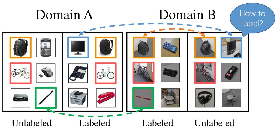
Figure 1: An illustration of weakly supervised open-set domain adaptation for domain collaboration. In each domain, there are some labeled and unlabeled samples. The frame colors represent the class of each item, while the unknown-class items have black frames. Without domain collaboration, the blue-framed item in Domain B cannot be classified properly because there are no labeled blue-framed data in its own domain. This is the same for the green-framed item in Domain A. (Best viewed in color)

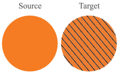
(a) Closed-set

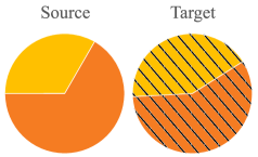
(b) Open-set

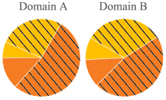
(c) Weakly Supervised Open-set

Figure 2: (a) closed-set domain adaptation, which assumes that the source and target domains contain the same set of interested classes (orange), and the two domains are either fully labeled (pure color), or unlabeled (with shade). (b) open-set domain adaptation [2], which allows both domains to contain unknown-class images (yellow). (c) weakly supervised open-set domain adaptation, in which both domains are scarcely labeled, with unknown-class images included. (Best viewed in color)

In conventional domain adaptation, the label spaces of the source and target domains are identical. However, such a setting may be restricted in applications. Recently in [2], open-set domain adaptation was proposed, where there exist samples in the target domain that do not belong to any class in the source domain, and vice versa. These samples cannot be represented by any class in the known label space, and they are therefore aggregated to an additional unknown class. One of our main goals is to detect these unknown-class samples in the target domain and in the meantime still classify the remaining known-class samples.

Moreover, in real applications, there often exists a large number of partially labeled datasets, where we cannot always find an off-the-shelf source dataset. Therefore, in the absence of an ideally large source domain, it is meaningful to perform domain adaptation collaboratively between these partially labeled domains. Hence, we consider the open-set domain adaptation together with the partially labeled datasets, which we call weakly supervised open-set domain adaptation. The differences between our setting and the existing ones are illustrated in Figure 2.

The weakly supervised open-set domain adaptation is practical whenever research or commercial groups need to collaborate by sharing datasets. This situation often happens when two groups each collected a large dataset in related areas, but each of them has only annotated a subset of all the item classes of interest (see Figure 1). To fully label the collected datasets, the groups need to share their datasets and let them learn from each other, which exactly fits our proposed setting, while traditional domain adaptation settings are not applicable.

Moreover, the proposed setting is practical when collecting a large source domain is unrealistic. This is often the case in real applications, as it is difficult to find large labeled data for items that only appear in specific tasks, which makes existing domain adaptation methods not applicable. For example, in person re-identification (see Section 4.2), it is impossible to find off-the-shelf labeled datasets for person identities captured by a certain camera view. Under this situation, one can let partially labeled datasets collected in different circumstances (e.g., data collected by different camera views) help label each other, for which our proposed setting is very suitable.

A key challenge of solving the weakly supervised open-set domain adaptation problem is how to perform domain adaptation when there only exists a small quantity of labeled data in both domains. To address this challenge, we propose to align two domains in a collaborative fashion. By implementing a novel dual mapping method, i.e., learning domain-specific feature transformations for each domain, we iteratively map the feature spaces of two domains $\mathcal{D_{A}}$ and $\mathcal{D_{B}}$ onto a shared latent space. To alleviate the effect of the unknown class, during the dual mapping optimization, we simultaneously maximize the margin between known-class and unknown-class samples , along with minimizing feature distribution discrepancy and intraclass variation . Therefore, we are able to obtain more robust unknown detection under the open-set setting . In addition, to enrich the discriminant ability, we propose to enlarge the label set by making pseudo-label predictions for the unlabeled samples, which are further selected by information entropy and used in dual-mapping optimization. After the domains are aligned in the shared latent space, we finally learn a classifier with labeled data from both domains. We call the above process that covers all the main challenges the Collaborative Distribution Alignment (CDA) method. Figure 3 shows an overview of our method.

The contributions of our paper are as follows:

1. We proposed the weakly supervised open-set domain adaptation, which allows partially labeled domains to be fully annotated by learning from each other. This setting extends domain adaptation to the scenarios where an ideal source domain is absent.

2. We proposed a collaborative learning method to address the proposed problem, which is well designed to handle the challenges introduced by both weakly supervised and open-set settings.

3. We evaluated our method on the standard domain adaptation benchmark Office and a real-world person re-identification application and showed its effectiveness.

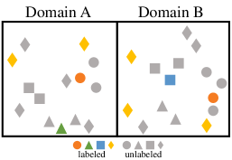
(a) Original Domains

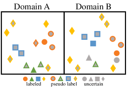
(b) Pseudo-Label Assignment

(c) Transformed Domains

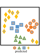
(d) Latent Space

Figure 3: An overview of our approach. In (a), labeled samples from different classes are filled with corresponding colors, while the gray samples are unlabeled. The shape of each sample indicates its ground-truth class. Specifically, the diamond-shaped samples represent the unknown-class samples. Note that the unknown-class samples are those that cannot be represented in the known label space, while the unlabeled samples are those without label information. Therefore, an unknown-class sample can be either labeled or unlabeled. In (b), we assign pseudo-labels (represented by frame colors) for some unlabeled samples, while excluding the remaining uncertain samples as outliers. In (c), we learn a set of domain-specific mappings that transform samples onto a latent domain, where domain discrepancy is reduced, same-class samples are aggregated, and separations between unknown and known class samples are formed. We then use the transformed features to update pseudo-labels in (b) and iterate between (b) and (c) until convergence. Finally, in the latent space shown in (d), we use a base classifier to annotate all the unlabeled samples, which we expect to be predicted as one of the known classes (red, green, and blue), or as an unknown-class sample (yellow). (Best viewed in color)

2 Related Works

Conventional Domain Adaptation. Domain adaptation is an important research area in machine learning. The core task of standard domain adaptation is to transfer discriminative knowledge from one fully labeled source domain to a scarcely labeled or unlabeled target domain [33]. A large number of methods have been proposed to solve this problem. A main stream of these works is to align the feature distributions of different domains onto a latent space. Along these lines, TCA [32] and JDA [28] were proposed to explicitly align marginal or joint distributions, while several models further extended the distribution alignment with structural consistency or geometrical discrepancy [16, 47]. Several recent works also introduced dataset shift losses to train deep networks that learn domain-invariant features [26, 29, 30, 42]. Another stream of work focuses on learning a subspace where both domains have a shared representation. SA [9] was proposed to align the PCA subspace, while CORAL [39] utilizes second-order statistics to minimize domain shift. Manifold learning was also conducted to find a geodesic path from the source to target domain [11, 13]. More recently, various generative adversarial models have been proposed [7, 17, 36, 41], in which feature extractors are trained to generate features for target samples that are not discriminated from the source samples. Although these methods are state-of-the-art for conventional domain adaptation tasks, none of them can directly tackle the weakly supervised open-set domain adaptation problem. On one hand, many of these methods require a fully labeled domain as a source, which does not exist in our setting. On the other hand, all of them are designed for the setting where the label spaces are identical, while in our setting, the label spaces of the two domains are overlapping but not identical. Thus, the performances of these methods are hindered by the unknown-class samples in each domain. In contrast, our proposed method is well designed for scarcely labeled domain pairs under the open-set setting.

Open-set Setting. In real-word application, the unknown impostors, which cannot be represented by any class in the label space of known classes, could significantly influence the overall performance. This problem has been receiving attention in the field of open-set object recognition [23, 37]. A typical solution is the OSVM [18], in which impostors are detected by estimating the inclusion probability. In the context of person re-identification, Zheng et al. proposed to explicitly learn a separation between a group of nontarget and target people [51]. Recently, Busto and Gall proposed the open-set setting for domain adaptation [2]. Their solution is to iteratively associate target samples with potential labels and map samples from the source domain to target domain, in which the unknown class is regarded as a normal class. More recently, the proposed OpenBP [36] adversarially learn s a decision boundary for the unknown class. In contrast to these methods, we explicitly construct large margins between the known and unknown class samples and in the meantime ensure that the unknown-class samples are not aligned between domains. Therefore, we can detect unknown-class samples more robustly.

Multi-task Learning. Our collaborative distribution alignment is a bilateral transfer, which is related to multi-task learning [48]. Through multi-task learning, tasks collaborate by sharing parameters [21, 27, 31] or features [5, 22], while in our method, domain collaboration is achieved by directly sharing data. Further, one may simply tackle the weakly supervised open-set domain adaptation problem with two tasks, each of which aims at training an independent classifier for a single domain. However, as illustrated in Figure 1, without the sharing of cross-domain data, many samples cannot be properly labeled. On the other hand, if we train a single classifier with shared data, the problem degenerates to single-task learning.

3 Collaborative Distribution Alignment

3.1 Approach Overview

To address the weakly supervised open-set domain adaptation problem, we aim to learn a shared latent space in which samples from different domains are well aligned. Suppose that we have two different domains $\mathcal{D_{A}}$ and $\mathcal{D_{B}}$, both of which have partially labeled samples. Let $\{\mathcal{D}_{i}=\mathcal{L}_{i}\bigcup\mathcal{U}_{i}\}_{i=A,B}$, where $\mathcal{L}_{i}=\{(x_{i}^{j},y_{i}^{j})\}_{j=1}^{l_{i}}$ denotes the labeled set with sample $x_{i}^{j}\in\mathbb{R}^{d}$ and label $y_{i}^{j}$, and $\mathcal{U}_{i}=\{(x_{i}^{j})\}_{j=l_{i}+1}^{l_{i}+u_{i}}$ is the unlabeled portion with unlabeled samples. Here, $x$ is the $d$-dimensional feature representation of each image sample, while $l_{i}$ and $u_{i}$ represent the sizes of $\mathcal{L}_{i}$ and $\mathcal{U}_{i}$, respectively. In practice, we have $l_{i}<<u_{i}$. Given a set $\mathcal{C}_{i}$ in labeled portion $\mathcal{L}_{i}$, which includes ${\color[rgb]{0,0,0}|\mathcal{C}_{i}|}-1$ known classes and an additional unknown class that gathers instances from all the classes that cannot be found in the known label space, our goal is to label each sample in $\mathcal{U}_{i}$ with a known class or detect it as an unknown-class sample.

From Figure 3(a), we can see that some samples in $\mathcal{U}_{A}$ do not belong to $\mathcal{C}_{A}$ but to $\mathcal{C}_{B}$. For example, there are unlabeled square samples in Domain A, but no labeled square sample exists in this domain. Merely using $\mathcal{L_{A}}$, we cannot properly label these samples. We then leverage the total labeled set $\mathcal{L}$, which consists of the labeled set $\mathcal{L}_{A}$ and $\mathcal{L}_{B}$ with the classes $\mathcal{C_{L}}=\mathcal{C_{A}}\bigcup\mathcal{C_{B}}$, to label all the samples in $\mathcal{U}_{A}$ and $\mathcal{U}_{B}$ as one of the classes in $\mathcal{C_{L}}$. However, due to domain shift between $\mathcal{D_{A}}$ and $\mathcal{D_{B}}$, direct ly using $\mathcal{L}$ would cause significant performance degeneration [33]. To solve this problem under our proposed setting, we focused on the following two most important features of our setting, which have not been well studied before:

1) Under the weakly supervised setting, we need to transfer knowledge bilaterally. Thus, for the first time, we introduce dual mapping (learning dual domain-specific mappings) into the domain adaptation area. Dual mapping can better exploit domain-specific information and align both domains onto the shared latent space (see Table 4).

2) Under the open-set setting, there could be a large number of unknown-class samples. To avoid confusing these samples with known-class ones, we are the first in domain adaptation to explicitly form large margins between known-class and unknown-class samples (Eq.3).

In general, our method works as follows. In each iteration, we first assign pseudo-labels to a subset of samples in $\mathcal{U_{A}}$ and $\mathcal{U_{B}}$. Then, we use the estimated pseudo-labels as well as the labeled set $\mathcal{L}$ to learn optimized values $W_{A}^{\prime}$ and $W_{B}^{\prime}$. Next, $\mathcal{D_{A}}W_{A}^{\prime}$ and $\mathcal{D_{B}}W_{B}^{\prime}$ are used to update the pseudo-labels, and a new iteration starts. This circle continues until it converges. After the termination, any base classifiers (SVM, k-NN) can be trained on $\mathcal{L_{A}}W_{A}$ and $\mathcal{L_{B}}W_{B}$ and predict labels for $\mathcal{U_{A}}W_{A}$ and $\mathcal{U_{B}}W_{B}$. We expect that the domain shift has been largely alleviated by performing this iterative optimization. The whole process is shown in Figure 3 and detailed in the following sections.

3.2 Pseudo-Label Assignment

Label Prediction. In the real world, there are usually much fewer labeled samples than unlabeled ones. With the scarce labeled samples, we are not able to robustly perform the subsequent optimization of $W_{A}$ and $W_{B}$. Therefore, to enlarge the label information set, we propose to first estimate the pseudo-labels of samples from $\mathcal{U}_{A}$ and $\mathcal{U}_{B}$. This can be easily done by applying base classifiers trained on $\mathcal{L}$ to predict labels of $\mathcal{U}_{A}$ and $\mathcal{U}_{B}$. This base classifier can be either k-NN, standard or variants of SVM, or neural networks. In our method, we simply utilize the standard linear SVM (LSVM) with probability estimation in the libsvm package [4] due to its wide use in domain adaptation works [2, 24, 39, 45].
Outlier Detection. However, due to domain discrepancy, some of the pseudo-labels are assigned uncertainly, and therefore, false estimation would result. We need to eliminate those uncertain labels from the optimization step in order to avoid iterative propagation of false estimations. As we have gained probability distribution estimations for each sample from LSVM, we propose to leverage information entropy $H$ to estimate the certainty of the prediction for each sample. A higher $H$ means that the probability distribution is more sparse, indicating that this prediction is more likely to be false. Therefore, we tend to only use samples with relatively low information entropy in the mapping step. Let $x_{i}$ be the $i^{th}$ sample and $C$ be the total number of classes, and $\textbf{Y}_{ij}$ is the probability of $x_{i}$ belonging to class $j$, given by LSVM. The information entropy of this prediction is denoted as

$$H(x_{i})=-\sum_{j=1}^{C}\textbf{Y}_{ij}log(\textbf{Y}_{ij}).$$ (1)

Then, if $H(x_{i})\geq\gamma$, we mark $x_{i}$ as an outlier that will not be used for dual mapping; otherwise, $x_{i}$ will be used. Here, $\gamma$ is an auto-adaptive threshold, which is set to the mean value of $H$ over all the samples. In the next iteration, all the unlabeled samples will be regarded equally again. Please note that unknown-class samples that are not close to any of the labeled samples would more likely be detected by this process for their low confidence.

3.3 Dual Mapping Under Open-set Condition

We intend to perform the dual mapping process by learning $W_{A},W_{B}\in{\color[rgb]{0,0,0}\mathbb{R}}^{d\times d}$ for $\mathcal{D_{A}}$ and $\mathcal{D_{B}}$, respectively. It is expected that $W_{A}$ and $W_{B}$ are able to map $\mathcal{D_{A}}$ and $\mathcal{D_{B}}$ onto a shared latent space. By learning these domain-specific matrices, we can better exploit domain-specific information for the two domains. This is different from most domain adaptation methods that only learn a single transform to transfer samples between domains [2, 28, 32, 39]. In Section 4, we have also empirically found that learning domain-specific transformation is more flexible for solving the weakly supervised open-set domain adaptation, as both domains play equal roles in this problem.

Known-Unknown Class Separation. Under the open-set setting, a main task is to detect and separate the unknown-class samples [2]. If there is no robust separation between known and unknown class samples, the overlapping of the known and unknown class samples would probably cause the problem of labelling a known-class sample as an unknown impostor, or vice versa. This significantly degenerates the overall performance. To solve this problem, we propose to encourage each known-class sample to be closer to its class center than to any of the unknown-class samples by a large margin.

To begin, we first compute the distances of each known-unknown sample pair in the transformed space. For each known-class sample $x$ in domain $D$ $\in$ {$A$, $B$}, we find its nearest unknown-class neighbor $x_{u}$, which is the unknown-class sample with the smallest distance from $x$. We formally define this distance as $f_{u}(x)=\left\|xW_{D}-x_{u}W_{D^{\prime}}\right\|^{2}_{F}$, where $D^{\prime}$ is the domain that $x_{u}$ belongs to. Similarly, we define the distance between $x$ and its class center $\overline{x}_{D}^{c}$ as $f_{c}(x)=\left\|(x-\overline{x}_{D}^{c})W_{D}\right\|^{2}_{F}$. We hope that for every $x$, we have

$$f_{c}(x)+1<f_{u}(x),$$ (2)

where 1 is the margin parameter that sets the scale of $W_{A}$ and $W_{B}$ [43]. We define $\mathcal{C}_{K}$ as the set of all the known classes and $\textbf{X}_{D}^{c}$ as the sample set of class $c$ in domain $D$. Then, the loss function for unknown separation in domain $D$ can be defined as

$$U_{D} =\sum\limits_{c\in\mathcal{C}_{K},x^{i}\in\textbf{X}_{D}^{c}}\left[1+f_{c}(x^{i})-f_{u}(x^{i})\right]_{+},$$ (3)

where the term $[x]_{+}=\max\{x,0\}$ is the standard hinge loss, which allows us to only penalize the unknown impostors that are inside the safety margin of $x$ and $\overline{x}_{D}^{c}$. For unknown-class samples that are far enough, the hinge loss becomes $0$ and does not contribute to $U_{D}$. The total unknown separation loss of $\mathcal{D_{A}}$ and $\mathcal{D_{B}}$ is defined as

$$U=\frac{1}{2}(U_{A}+U_{B}).$$ (4)

Aligning Known-class Samples between Domains. Under the open-set setting, aligning all samples between two domains is unnecessary because the purpose of dual mapping is to align all the known-class samples to gain a better classification performance while dragging all the unknown-class samples away from the known ones to make a clear separation.

To this end, we discard all the unknown class samples in the distribution alignment process for domain adaptation. To measure the domain discrepancy, we adopt the maximum mean discrepancy (MMD) [1], which is a widely used nonparametric domain discrepancy measurement in domain adaptation works [26, 28, 32, 42].

More specifically, the marginal distribution distance between the transformed domains can be computed by

$$Dist_{M}=\frac{1}{2}\left\|P_{A}W_{A}-P_{B}W_{B}\right\|^{2}_{F},$$ (5)

where $P_{D}=\frac{1}{n^{k}_{D}}\sum_{i=1}^{n_{D}^{k}}x_{D}^{i}$ is the mean of known samples in domain $D$, and $n_{D}^{k}$ denotes the number of those samples. Similarly, the distance between conditional distributions $Dist_{C}$ can be measured by the sum of the distances between the corresponding known class centers in both domains. That is defined as

$$Dist_{C}=\frac{1}{2}\sum_{c\in\mathcal{C}_{K}}\left\|P_{A}^{c}W_{A}-P_{B}^{c}W_{B}\right\|^{2}_{F},$$ (6)

where $P_{D}^{c}=\frac{1}{n_{D}^{c}}\sum_{i=1}^{n_{D}^{c}}x_{D}^{c,i}$ is the mean of class $c$ samples, and $x_{D}^{c,i}$ is the $i^{th}$ sample of class $c$ in domain $D$. The label of each sample is either provided by the dataset or assigned by pseudo-label prediction.

By minimizing $Dist_{M}$ and $Dist_{C}$, the discrepancies between both marginal and conditional distributions of known-class samples in $\mathcal{D_{A}}$ and $\mathcal{D_{B}}$ are reduced, while the unknown-class samples will not be improperly aligned.

Aggregating Same-class Samples. To facilitate the center-based separation between known and unknown class samples (Eq.4) as well as the alignment between known class samples based on MMD (Eq.6), we propose to explicitly aggregate all the samples to their class centers.

In detail, we define $\overline{x}_{D}^{c}$ as the estimated center of class $c$ in domain $D$ and $\textbf{X}_{D}^{c}$ as the sample set of class $c$ with size $n_{D}^{c}$. Then, the aggregation loss function $G_{D}$ can be expressed by

$$G_{D}=\sum_{c\in\mathcal{C_{L}}} \frac{1}{n_{D}^{c}}\sum_{x^{i}\in\textbf{X}_{D}^{c}}\left\|(x^{i}-\overline{x}_{D}^{c})W_{\color[rgb]{0,0,0}D}\right\|^{2}_{F}.$$ (7)

Overall, the total loss $G$ of $\mathcal{D_{A}}$ and $\mathcal{D_{B}}$ is then defined as

$$G=\frac{1}{2}(G_{A}+G_{B}).$$ (8)

Objective Function. With all the components discussed above, our method can be formed now. To configure the strength of each component, we introduce balancing parameters $\lambda_{M},\lambda_{G},\text{ and }\lambda_{U}$ for marginal distribution alignment, center aggregation and known-unknown class separation, respectively. We define the total loss function as

$$\begin{aligned} f=Dist_{C}+\lambda_{M}Dist_{M}+\lambda_{G}G+\lambda_{U}U\end{aligned}.$$ (9)

Then, our objective function can be concluded as follows:

$$(W_{A}^{*},W_{B}^{*})=\mathop{\arg\min}_{W_{A},W_{B}}f(\mathcal{D_{A}},\mathcal{D_{B}},W_{A},W_{B}).$$ (10)

Details of the optimization process are given in the supplementary material due to lack of space.

4 Experiments

4.1 Office Dataset

The Office dataset [35] is a standard benchmark for domain adaptation evaluation [2, 26, 39, 36] and consists of three real-word object domains: Amazon (A), Webcam (W) and DSLR (D). In total, it has 4,652 images with 31 classes. We construct three dual collaboration tasks: A $\leftrightarrow$ W, A $\leftrightarrow$ D and W $\leftrightarrow$ D, where $\leftrightarrow$ denotes the collaboration relation between two domains. Similar to [2], we extract the features using ResNet-50 [14] pretrained on ImageNet [6]. For parameters, we set $\lambda_{M}=10,\lambda_{G}=1$ and $\lambda_{U}=0.1$.

Protocol. We randomly selected 15 classes as the known classes, and the remaining classes are set as one unknown class, i.e., there are 16 classes in total. Both domains contain all 16 classes, while only a subset of them have labeled samples. Specifically, we randomly selected 10 known classes to form the labeled known-class set for each domain, with the constraint that 5 classes are shared between them. Similar to [2], for each domain, we randomly took 3 samples from each class in the labeled known-class set and 9 samples from the unknown class, as labeled samples, and set all the remaining as unlabeled. We expect each unlabeled sample to be correctly labeled either as one of the 15 known classes or the unknown class. The above is repeated 5 times, and the mean accuracy and standard deviation of each method are reported.

Compared Methods. We first compared the proposed CDA with two open-set domain adaptation methods, ATI [2] and OpenBP [36]. The conventional unsupervised domain adaptation methods, including TCA [32], GFK [11], CORAL [39], JAN [30] and PADA [3], are compared as well. Since our method learns dual projections, to undertake a fair comparison, for methods that require a single labeled domain (ATI, OpenBP, JAN, and PADA), we apply them by two steps: given $\mathcal{L_{A}}$ as the source and $\mathcal{D_{B}}$ as the unlabeled target, we learn to transform $\mathcal{L_{A}}$ to $\mathcal{D_{B}}$, and label $\mathcal{U_{B}}$ with $\mathcal{L_{A}}$ and $\mathcal{L_{B}}$. Then, we learn to label $\mathcal{U_{A}}$ in a symmetrical way. For other methods, we simply transform $\mathcal{D_{A}}$ to $\mathcal{D_{B}}$.

Since there are a small number of labeled samples in the target domain for semi-supervised domain adaptation, we also compared two semi-supervised methods, namely MMDT [15] and ATI-semi [2]. We test these methods in a way similar to methods such as ATI and JAN, except the target domain in each symmetry step here is semi-supervised.

In addition, we compared multi-task learning methods since our method benefits from the collaborative transfer between two domains, which is related to multi-task learning. For compariso n, we report the results of CLMT [5], AMTL [21], and MRN [27]. By following [5, 21], every task in CLMT and AMTL is set as a one-vs-all binary classification problem. For MRN, we denote two tasks as learning classifiers on $\mathcal{D_{A}}$ and $\mathcal{D_{B}}$, separately.

The results of the above methods are obtained by linear SVM and trained and tested on transformed features, except for CLMT and AMTL, which directly learn classifiers. As baselines, we report results of the LSVM trained with non-adaptation data $\mathcal{L}$, which we call NA. We also report another baseline called NA-avg, which is the average accuracy of training and testing a LSVM for each domain independently. Moreover, we have also undertaken a comparison with methods in [9, 10, 26, 28, 40, 47, 42], the results of which are less competitive and are thus only included in the supplementary material for sake of space.

Methods	A $\leftrightarrow$ W	A $\leftrightarrow$ D	W $\leftrightarrow$ D	AVG.
NA-avg	62.2 $\pm$ 3.19	61.0 $\pm$ 3.05	66.3 $\pm$ 1.72	63.12
NA	72.6 $\pm$ 2.04	69.4 $\pm$ 2.22	84.2 $\pm$ 3.89	75.40
TCA [32]	73.3 $\pm$ 1.67	70.6 $\pm$ 1.99	83.5 $\pm$ 3.96	75.80
GFK [11]	56.9 $\pm$ 2.89	55.7 $\pm$ 1.46	70.9 $\pm$ 4.85	61.17
CORAL [39]	69.9 $\pm$ 4.41	67.7 $\pm$ 3.13	83.7 $\pm$ 3.65	73.77
JAN [30]	63.8 $\pm$ 1.27	65.5 $\pm$ 0.76	74.7 $\pm$ 1.41	68.00
PADA [3]	60.3 $\pm$ 1.09	60.2 $\pm$ 0.98	70.9 $\pm$ 1.88	63.80
ATI [2]	70.4 $\pm$ 4.15	65.9 $\pm$ 1.80	81.7 $\pm$ 4.74	72.67
OpenBP [36]	62.6 $\pm$ 4.11	62.9 $\pm$ 1.71	67.9 $\pm$ 2.31	64.47
ATI-semi [2]	73.4 $\pm$ 2.28	72.0 $\pm$ 2.87	77.8 $\pm$ 3.40	74.72
MMDT [15]	72.6 $\pm$ 2.15	69.4 $\pm$ 2.19	84.4 $\pm$ 3.99	75.47
AMTL [21]	50.2 $\pm$ 1.45	48.8 $\pm$ 0.90	62.1 $\pm$ 2.17	53.70
CLMT [5]	50.3 $\pm$ 1.47	50.0 $\pm$ 0.77	61.7 $\pm$ 1.23	54.00
MRN [27]	62.2 $\pm$ 3.38	62.4 $\pm$ 2.44	77.4 $\pm$ 3.43	67.33
CDA	77.1 $\pm$ 1.35	75.2 $\pm$ 1.63	88.1 $\pm$ 2.45	80.13

Table 1: Comparing state-of-the-art methods on Office. The $1^{\text{st}}/2^{\text{nd}}$ best results are indicated in red/blue.

Method	1 $\leftrightarrow$ 2		2 $\leftrightarrow$ 3		3 $\leftrightarrow$ 4		4 $\leftrightarrow$ 5		5 $\leftrightarrow$ 6		6 $\leftrightarrow$ 7		7 $\leftrightarrow$ 8		8 $\leftrightarrow$ 1		AVG.
	r=1	r=5	r=1	r=5	r=1	r=5	r=1	r=5	r=1	r=5	r=1	r=5	r=1	r=5	r=1	r=5	r=1	r=5
NA-avg	43.6	55.3	29.6	38.2	50.1	54.8	69.2	95.2	38.2	54.4	33.5	42.4	22.0	40.3	76.7	95.4	45.4	59.5
NA	59.3	75.1	41.4	53.2	64.4	78.8	74.1	98.9	49.0	67.1	51.9	65.4	27.6	49.6	78.3	98.9	55.7	73.4
TCA [32]	58.6	74.7	41.0	53.7	64.3	79.0	75.3	98.9	48.6	67.3	51.5	65.3	27.2	49.8	78.3	98.9	55.6	73.5
GFK [11]	59.1	75.1	41.5	53.5	64.5	79.0	75.3	99.0	49.0	67.4	51.9	65.5	27.7	50.3	78.5	98.9	55.9	73.6
CORAL [39]	58.9	75.8	41.6	54.2	64.2	78.4	74.5	98.8	47.7	66.3	51.5	64.6	26.5	48.6	78.4	98.8	55.4	73.2
JAN [30]	24.0	43.7	34.4	64.4	21.4	38.6	75.5	90.2	30.2	60.0	27.7	52.4	44.6	72.1	81.7	92.5	42.4	64.2
PADA [3]	14.0	30.7	39.4	62.2	22.1	35.3	75.4	89.0	30.1	57.4	27.2	50.4	47.4	70.9	77.6	91.1	41.6	60.9
ATI [2]	58.6	74.0	40.6	49.5	65.4	79.2	36.1	78.0	47.9	63.6	52.4	65.6	24.6	42.7	28.2	84.4	44.2	67.1
OpenBP [36]	34.7	49.7	45.9	66.5	27.3	39.8	77.1	90.6	8.1	26.5	37.6	53.5	47.5	67.3	83.5	93.3	45.2	54.9
MRN [27]	26.2	46.5	19.2	32.8	34.0	49.6	74.9	94.4	25.9	49.9	24.4	43.1	19.9	50.2	53.6	85.1	34.8	56.5
ATI-semi [2]	53.4	71.8	55.6	71.8	56.5	76.8	39.7	88.9	55.3	69.3	57.6	76.9	46.7	65.6	30.6	86.3	49.4	75.9
MMDT [15]	36.0	51.1	35.7	51.5	57.5	73.2	74.2	98.9	29.2	53.2	22.0	39.5	19.1	43.5	76.5	98.6	42.9	62.3
LMNN [43]	59.4	78.1	42.5	59.1	61.8	74.1	84.7	96.3	53.3	72.2	50.8	66.1	33.5	60.8	90.2	97.7	59.5	75.5
KISSME [20]	55.2	68.6	49.2	71.0	63.1	75.3	86.0	94.9	57.6	74.5	55.3	71.6	45.8	71.6	22.0	56.7	54.3	73.0
XQDA [25]	55.6	68.9	49.1	71.0	63.1	75.3	86.0	94.9	57.6	74.5	55.3	71.6	45.8	71.6	48.2	86.0	57.6	76.7
DLLR [19]	59.2	75.0	41.3	52.9	64.1	78.1	72.9	98.7	48.7	66.9	51.8	64.5	27.9	49.6	78.5	99.0	55.6	73.1
SPGAN [7]	41.6	59.9	31.3	47.5	44.7	58.6	69.6	97.7	41.4	61.0	43.3	59.6	22.8	46.3	74.1	98.0	48.7	69.6
CDA	64.6	80.4	62.4	88.1	67.9	84.9	76.0	98.9	61.5	82.1	59.6	78.1	67.2	83.8	85.6	98.5	68.1	86.9

Table 2: Comparing CMC accuracies with state-of-the-art methods on DukeMTMC-reID (%).

Comparison Results. The results are shown in Table 1. We can observe that our proposed CDA method outperforms all the other methods in the three tasks. For example, CDA respectively surpasses the best alternative TCA by 3.8%, 4.6% and 4.6% in A$\leftrightarrow$W, A$\leftrightarrow$D and W$\leftrightarrow$D, respectively. Further, CDA exceeds TCA by 4.33% (80.13%-75.80%) on average. The reasons may be as follows. (1) Unlike closed-set methods (such as TCA) that align distributions over all the samples, our CDA is well designed to only align feature distributions of the known classes. By doing so, we avoid a negative transfer caused by aligning distributions of the unknown class, the samples of which may actually come from different classes with inherently different features. (2) CDA learns more discriminative features by minimizing intraclass variation and explicitly separating known and unknown class samples, while most other methods only focus on learning domain-invariant features. (3) CDA simultaneously exploits unlabeled information in both domains, while other methods that require a fully labeled source domain (such as ATI) only use unlabeled data in a single domain in each symmetry step.

Additionally, our method outperformed semi-supervised domain adaptation methods. This could be because we simultaneously utilize unlabeled data from both domains, while these methods use them separately. Moreover, CDA largely exceeds multi-task learning methods, which occurs mainly because (1) CDA aligns both domains, but AMTL and CLMT ignore the domain discrepancy in training samples and because (2) CDA merges incomplete label spaces of $\mathcal{L_{A}}$ and $\mathcal{L_{B}}$ to form a complete one, while in MRN, these label spaces are separated.

4.2 Person Re-identification (re-id) Application

A natural practical example of our proposed setting can be the person re-identification (re-id) problem [12], which is widely and deeply researched in computer vision for visual surveillance [7, 8, 46, 51]. Re-id aims to match people’s images across nonoverlapping camera views. Currently, training state-of-the-art re-id models requires a large number of cross-camera labeled images [20, 25, 43], but it is very expensive to manually label (pairwise) people images across cameras views. Further, as mentioned before, we cannot find an off-the-shelf source domain for these people. Thus, it is meaningful to annotate images in each camera pair by performing domain adaptation collaboratively between these camera views. Moreover, it is hard to guarantee that people appearing in one camera view would also appear in another view. This problem introduces the open-set setting. Therefore, to show the practicality of the proposed setting and the effectiveness of CDA, we conduct an experiment on a real-world re-id application in this subsection.

DukeMTMC-reID [34] is a popular re-id benchmark [7, 8, 38, 44]. It consists of person images from 8 nonoverlapping camera views. The DukeMTMC-reID dataset is a genuine open-set re-id dataset, since for each camera pair, there are a number of identities that only appear in one view and thus lack an image to match in another view. For example, in camera pair 1 $\leftrightarrow$ 2, there are 105 identities unique to camera 1 and 84 identities unique to camera 2. For evaluation, we conducted our experiments on the largest portion gallery. We constructed 8 camera pairs for our experiment, where each camera view appears twice, and extracted features with ResNet-50 that was pretrained on Market-1501 [49] using the method in [50]. For parameters, we set $\lambda_{M}=10,\lambda_{G}=1$, and $\lambda_{U}=1$.

Protocol. For both camera views, we let the classes that only appear in a single camera view belong to the unknown class, while the shared classes are set as known classes. To simulate the weakly supervised setting, in each camera view, all the known classes exist, but only a subset of them have labeled samples. We call the set of known classes that have labeled samples the labeled known-class set. Suppose there are $N$ known classes. Then, for each camera view, we randomly select 2$N$/3 known classes to form its labeled known-class set, with the constraint that $N$/3 classes are shared between these sets of both views. Then, for each view, we randomly take 1 image as a labeled sample from each class in its labeled known-class set. Additionally, $N$/4 samples from the unknown class are labeled as well. All the rest are set as unlabeled. During testing, for each image in the unlabeled set, we retrieve the matched persons from the labeled set. Then, we use the cumulative match characteristic (CMC) to measure the re-id matching performance.

Compared Methods. We first evaluated all the methods mentioned in Section 4.1, except AMTL and CLMT, since they merely learn a classifier and are thus unsuitable for distance-based person re-id tasks. Moreover, we include common re-id oriented methods (1)LMNN [43], (2)KISSME [20], (3)XQDA [25], and (4) DLLR [19], as well as the newly proposed SPGAN [7]. To test SPGAN, for each pair, we use this model to transfer the image style of each sample in the first view to the other view and then evaluate on these transferred images. As baselines, we report results of directly computing Euclidean distances on the original space, namely, NA and NA-avg (similar to the baselines used in Section 4.1).

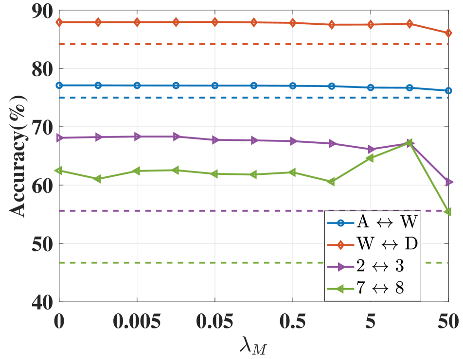
(a) $\lambda_{M}$

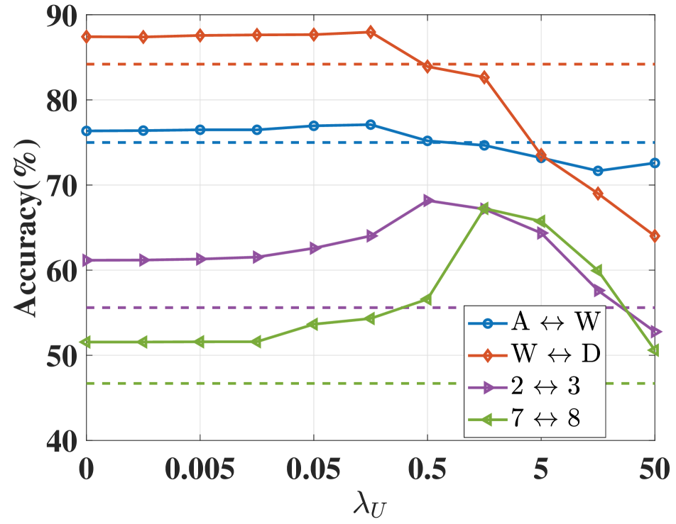
(b) $\lambda_{U}$

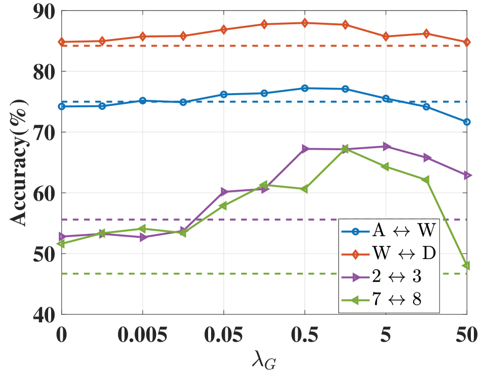
(c) $\lambda_{G}$

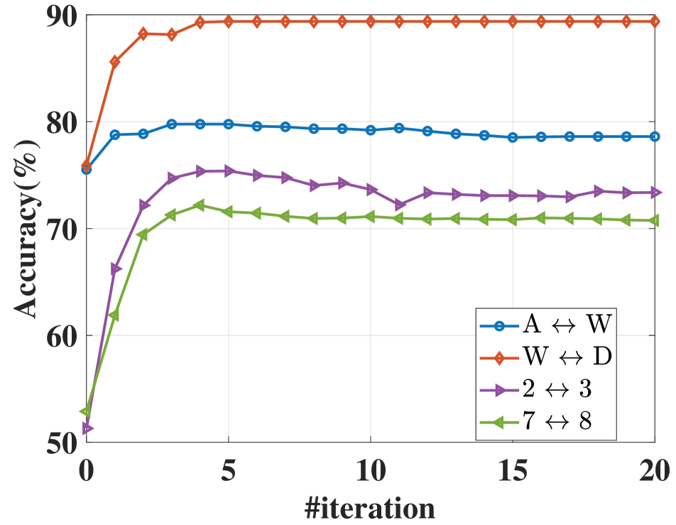
(d) convergence

Figure 4: Classification accuracy w.r.t. $\lambda_{M}$, $\lambda_{U}$, $\lambda_{\color[rgb]{0,0,0}G}$ in (a), (b), and (c), respectively, where the dashed lines represent the best state-of-the-art performances for each task. (d) illustrates the convergence of the proposed method.

Comparison Results. The results are shown in Table 2. Our method outperformed all the other methods in 6 of the 8 total tasks, for example, surpassing the best alternative LMNN by 5.2%, 19.9%, 8.2%, and 33.7% at rank-1 on 1$\leftrightarrow$2, 2$\leftrightarrow$3, 5$\leftrightarrow$6 and 7$\leftrightarrow$8, respectively. The performance margins over the other methods are larger still. On average, our method outperforms the most competitive methods by 8.6% (68.1%-59.5%) and 10.2% (86.9%-76.7%) at rank-1 and rank-5, respectively. It is obvious that CDA significantly outperformed NA and NA-avg, while almost all the compared methods at least once performed worse than the baselines due to negative transfer.

Compared to typical methods for re-id, CDA achieves better performance mainly because (1) CDA makes use of a large number of unlabeled samples by pseudo-label assignment, while LMNN, KISS and XQDA merely rely on labeled samples, and (2) CDA explicitly separates known and unknown-class samples, while the compared methods (such as SPGAN) do not distinguish these two kinds of samples. The superior performance of CDA in re-id further validates the effectiveness of the proposed method.

4.3 Further Analysis of CDA

Effect of Each Component. Our loss function in Equation 9 involves four components: the marginal and conditional distribution alignments ($Dist_{M}$, $Dist_{C}$), the intraclass aggregation ($G$), and the unknown-class sample separation ($U$). We empirically evaluated the importance of each component. For each component, we report the performance of the CDA model when each component is eliminated. The results are shown in Table 3. We can observe that the accuracy of CDA would drop once we remove any of the components. For example, on task 5$\leftrightarrow$6, the performance decreased by 11.7%, 4.2%, 38.4% and 1.2% when $G$, $U$, $Dist_{C}$, and $Dist_{M}$ was removed, respectively.

Models	A$\leftrightarrow$D	A$\leftrightarrow$W	W$\leftrightarrow$D	5$\leftrightarrow$6	7$\leftrightarrow$8
Missing $G$	70.0	73.5	84.7	49.8	51.6
Missing $U$	74.4	76.4	86.8	57.3	51.6
Missing $Dist_{C}$	64.9	70.3	79.4	23.1	11.2
Missing $Dist_{M}$	74.8	77.1	87.9	60.3	62.5
CDA	75.2	77.1	88.1	61.5	67.2

Table 3: Effect of components of Eq.9 (%)

Parameter Sensitivity. In this section, we evaluated the parameter sensitivity of our model. We run CDA with a large range of parameters $\lambda_{M}$, $\lambda_{U}$ and $\lambda_{\color[rgb]{0,0,0}G}$ from 0 to 50. The results of randomly chosen tasks are shown in Figure 4 on the two datasets used in our experiments. As shown, there should be a proper range for each parameter. Taking $\lambda_{U}$ for example, when $\lambda_{U}$ is too large, we mainly learn to separate known/unknown-class samples, making feature alignment weaker; when it is too small, we are not able to adequately separate known/unknown-class samples. Nevertheless, it can be observed that the performance of CDA is robust for $\lambda_{M}\in[0.001,10]$, $\lambda_{U}\in[{\color[rgb]{0,0,0}0.01},1]$, and $\lambda_{G}\in[0.5,10]$.

Convergence. We empirically tested the convergence property of CDA. The result in Figure 4 (d) shows that the accuracy increases and converges in approximately 5 iterations.

Effect of Outlier Detection. We detect and remove low-confidence pseudo-labels by setting a threshold of information entropy in Eq.1. To show the effectiveness of this process, we compared CDA with the CDA without outlier detection. As shown in the second and fourth rows of Table 4, all the tasks significantly benefit from this process, which shows the importance of the outlier detection.

Models	A$\leftrightarrow$D	A$\leftrightarrow$W	W$\leftrightarrow$D	5 $\leftrightarrow$ 6	7 $\leftrightarrow$ 8
no outlier	74.3	73.4	86.0	52.7	38.0
single mapping	70.2	69.8	81.1	56.5	33.9
CDA	75.2	77.1	88.1	61.5	67.2

Table 4: Effect of outlier detection and dual mapping (%)

Effect of Dual Mapping. To map each domain to the shared latent space, we learn a different transformation matrix for each domain. To compare this fashion with learning a shared transform matrix for both domains, we conducted CDA by learning the same transformation matrix for both domains. The results shown in Table 4 demonstrate the advantage of dual mapping. This outcome is probably because dual mapping enables learning more domain-specific information for each domain during the adaptation process.

Other Experiments. We have also performed experiments on the following aspects: (1) time complexity, (2) effect of different pseudo-labelling methods, (3) effect of the number of labeled samples in each domain and (4) effect of overlapping rate of known label spaces between the two domains. For the sake of space, descriptions and results of these experiments are given in the supplementary material.

5 Conclusion

In this paper, we introduced the weakly supervised open-set domain adaptation problem. This setting extends domain adaptation to the scenarios where an ideal source domain is absent, and we need to let partially labeled domains learn from each other. To address this problem, we propose a novel Collaborative Distribution Alignment approach. Compared to previous works, this study represents the first attempt to enhance overall performance by domain collaboration. Future works could be undertaken to detect the unknown-class samples more effectively or to design an adaptive neural network for end-to-end training.

6 Acknowledgement

This work was supported partially by NSFC (U1811461, 61522115), Guangdong Province Science and Technology Innovation Leading Talents (2016TX03X157).

References

- [1] Shai Ben-David, John Blitzer, Koby Crammer, and Fernando Pereira. Analysis of representations for domain adaptation. In Proceedings of Advances in Neural Information Processing Systems (NeurIPS), pages 137--144, 2007.
- [2] Pau Panareda Busto and Juergen Gall. Open set domain adaptation. In Proceedings of the IEEE International Conference on Computer Vision (ICCV), pages 754--763, 2017.
- [3] Zhangjie Cao, Lijia Ma, Mingsheng Long, and Jianmin Wang. Partial adversarial domain adaptation. In Proceedings of the European Conference on Computer Vision (ECCV), pages 135--150, 2018.
- [4] Chih-Chung Chang and Chih-Jen Lin. LIBSVM: A library for support vector machines. ACM Transactions on Intelligent Systems and Technology, 2:27:1--27:27, 2011.
- [5] Carlo Ciliberto, Youssef Mroueh, Tomaso Poggio, and Lorenzo Rosasco. Convex learning of multiple tasks and their structure. In Proceedings of the International Conference on Machine Learning (ICML), pages 1548--1557, 2015.
- [6] J. Deng, W. Dong, R. Socher, L. Li, Kai Li, and Li Fei-Fei. Imagenet: A large-scale hierarchical image database. In Proceedings of the IEEE conference on Computer Vision and Pattern Recognition (CVPR), pages 248--255, June 2009.
- [7] Weijian Deng, Liang Zheng, Qixiang Ye, Guoliang Kang, Yi Yang, and Jianbin Jiao. Image-image domain adaptation with preserved self-similarity and domain-dissimilarity for person re-identification. In Proceedings of the IEEE conference on Computer Vision and Pattern Recognition (CVPR), June 2018.
- [8] Hehe Fan, Liang Zheng, and Yi Yang. Unsupervised person re-identification: clustering and fine-tuning. arXiv preprint arXiv:1705.10444, 2017.
- [9] Basura Fernando, Amaury Habrard, Marc Sebban, and Tinne Tuytelaars. Unsupervised visual domain adaptation using subspace alignment. In Proceedings of the IEEE International Conference on Computer Vision (ICCV), pages 2960--2967, 2013.
- [10] Yaroslav Ganin and Victor Lempitsky. Unsupervised domain adaptation by backpropagation. In Proceedings of the International Conference on Machine Learning (ICML), pages 1180--1189, 2015.
- [11] Boqing Gong, Yuan Shi, Fei Sha, and Kristen Grauman. Geodesic flow kernel for unsupervised domain adaptation. In Proceedings of the IEEE conference on Computer Vision and Pattern Recognition (CVPR), pages 2066--2073. IEEE, 2012.
- [12] Shaogang Gong, Marco Cristani, Shuicheng Yan, and Chen Change Loy. Person re-identification. Springer, 2014.
- [13] Raghuraman Gopalan, Ruonan Li, and Rama Chellappa. Unsupervised adaptation across domain shifts by generating intermediate data representations. IEEE transactions on pattern analysis and machine intelligence, 36(11):2288--2302, 2014.
- [14] Kaiming He, Xiangyu Zhang, Shaoqing Ren, and Jian Sun. Deep residual learning for image recognition. In Proceedings of the IEEE conference on Computer Vision and Pattern Recognition (CVPR), pages 770--778, 2016.
- [15] Judy Hoffman, Erik Rodner, Jeff Donahue, Kate Saenko, and Trevor Darrell. Efficient learning of domain-invariant image representations. In Proceedings of International Conference on Learning Representations (ICLR), 2013.
- [16] Cheng-An Hou, Yao-Hung Hubert Tsai, Yi-Ren Yeh, and Yu-Chiang Frank Wang. Unsupervised domain adaptation with label and structural consistency. IEEE Transactions on Image Processing, 25(12):5552--5562, 2016.
- [17] Lanqing Hu, Meina Kan, Shiguang Shan, and Xilin Chen. Duplex generative adversarial network for unsupervised domain adaptation. In Proceedings of the IEEE conference on Computer Vision and Pattern Recognition (CVPR), June 2018.
- [18] Lalit P. Jain, Walter J. Scheirer, and Terrance E. Boult. Multi-class open set recognition using probability of inclusion. In David Fleet, Tomas Pajdla, Bernt Schiele, and Tinne Tuytelaars, editors, Proceedings of the European Conference on Computer Vision (ECCV), pages 393--409, Cham, 2014. Springer International Publishing.
- [19] Elyor Kodirov, Tao Xiang, and Shaogang Gong. Dictionary learning with iterative laplacian regularisation for unsupervised person re-identification. In Proceedings of the British Machine Vision Conference (BMVC), volume 3, page 8, 2015.
- [20] Martin Koestinger, Martin Hirzer, Paul Wohlhart, Peter M Roth, and Horst Bischof. Large scale metric learning from equivalence constraints. In Proceedings of the IEEE conference on Computer Vision and Pattern Recognition (CVPR), pages 2288--2295. IEEE, 2012.
- [21] Giwoong Lee, Eunho Yang, et al. Asymmetric multi-task learning based on task relatedness and confidence. In Proceedings of the International Conference on Machine Learning (ICML), pages 230--238, 2016.
- [22] Hae Beom Lee, Eunho Yang, and Sung Ju Hwang. Deep asymmetric multi-task feature learning. In Proceedings of the International Conference on Machine Learning (ICML), pages 2956--2964, 2018.
- [23] Fayin Li and H. Wechsler. Open set face recognition using transduction. IEEE Transactions on Pattern Analysis and Machine Intelligence, 27(11):1686--1697, Nov 2005.
- [24] Shuang Li, Shiji Song, and Gao Huang. Prediction reweighting for domain adaptation. IEEE transactions on neural networks and learning systems, 28(7):1682--1695, 2017.
- [25] Shengcai Liao, Yang Hu, Xiangyu Zhu, and Stan Z Li. Person re-identification by local maximal occurrence representation and metric learning. In Proceedings of the IEEE conference on Computer Vision and Pattern Recognition (CVPR), pages 2197--2206, 2015.
- [26] Mingsheng Long, Yue Cao, Jianmin Wang, and Michael I. Jordan. Learning transferable features with deep adaptation networks. In Proceedings of the International Conference on Machine Learning (ICML), pages 97--105, 2015.
- [27] Mingsheng Long, Zhangjie Cao, Jianmin Wang, and S Yu Philip. Learning multiple tasks with multilinear relationship networks. In Proceedings of Advances in Neural Information Processing Systems (NeurIPS), pages 1594--1603, 2017.
- [28] Mingsheng Long, Jianmin Wang, Guiguang Ding, Jia-Guang Sun, and Philip S. Yu. Transfer feature learning with joint distribution adaptation. Proceedings of the IEEE International Conference on Computer Vision (ICCV), pages 2200--2207, 2013.
- [29] Mingsheng Long, Han Zhu, Jianmin Wang, and Michael I. Jordan. Unsupervised domain adaptation with residual transfer networks. In Proceedings of Advances in Neural Information Processing Systems (NeurIPS), pages 136--144, 2016.
- [30] Mingsheng Long, Han Zhu, Jianmin Wang, and Michael I. Jordan. Deep transfer learning with joint adaptation networks. In Proceedings of the International Conference on Machine Learning (ICML), pages 2208--2217, 2017.
- [31] Ishan Misra, Abhinav Shrivastava, Abhinav Gupta, and Martial Hebert. Cross-stitch networks for multi-task learning. In Proceedings of the IEEE conference on Computer Vision and Pattern Recognition (CVPR), pages 3994--4003, 2016.
- [32] Sinno Jialin Pan, Ivor W Tsang, James T Kwok, and Qiang Yang. Domain adaptation via transfer component analysis. IEEE Transactions on Neural Networks, 22(2):199--210, 2011.
- [33] Sinno Jialin Pan, Qiang Yang, et al. A survey on transfer learning. IEEE Transactions on knowledge and data engineering, 22(10):1345--1359, 2010.
- [34] Ergys Ristani, Francesco Solera, Roger Zou, Rita Cucchiara, and Carlo Tomasi. Performance measures and a data set for multi-target, multi-camera tracking. In European Conference on Computer Vision workshop on Benchmarking Multi-Target Tracking, 2016.
- [35] Kate Saenko, Brian Kulis, Mario Fritz, and Trevor Darrell. Adapting visual category models to new domains. In Proceedings of the European Conference on Computer Vision (ECCV), pages 213--226. Springer, 2010.
- [36] Kuniaki Saito, Shohei Yamamoto, Yoshitaka Ushiku, and Tatsuya Harada. Open set domain adaptation by backpropagation. In Vittorio Ferrari, Martial Hebert, Cristian Sminchisescu, and Yair Weiss, editors, Proceedings of the European Conference on Computer Vision (ECCV), 2018.
- [37] W. J. Scheirer, A. de Rezende Rocha, A. Sapkota, and T. E. Boult. Toward open set recognition. IEEE Transactions on Pattern Analysis and Machine Intelligence, 35(7):1757--1772, July 2013.
- [38] Arne Schumann and Rainer Stiefelhagen. Person re-identification by deep learning attribute-complementary information. IEEE Conference on Computer Vision and Pattern Recognition Workshops (CVPRW), pages 1435--1443, 2017.
- [39] Baochen Sun, Jiashi Feng, and Kate Saenko. Return of frustratingly easy domain adaptation. In Proceedings of the Thirtieth AAAI Conference on Artificial Intelligence, AAAI, pages 2058--2065. AAAI Press, 2016.
- [40] Baochen Sun and Kate Saenko. Deep coral: Correlation alignment for deep domain adaptation. In Proceedings of the European Conference on Computer Vision (ECCV), pages 443--450. Springer, 2016.
- [41] Eric Tzeng, Judy Hoffman, Kate Saenko, and Trevor Darrell. Adversarial discriminative domain adaptation. In Proceedings of the IEEE conference on Computer Vision and Pattern Recognition (CVPR), volume 1, page 4, 2017.
- [42] Eric Tzeng, Judy Hoffman, Ning Zhang, Kate Saenko, and Trevor Darrell. Deep domain confusion: Maximizing for domain invariance. CoRR, abs/1412.3474, 2014.
- [43] Kilian Q Weinberger and Lawrence K Saul. Distance metric learning for large margin nearest neighbor classification. Journal of Machine Learning Research, 10(Feb):207--244, 2009.
- [44] Tong Xiao, Shuang Li, Bochao Wang, Liang Lin, and Xiaogang Wang. Joint detection and identification feature learning for person search. In Proceedings of the IEEE conference on Computer Vision and Pattern Recognition (CVPR), pages 3376--3385. IEEE, 2017.
- [45] Yuguang Yan, Wen Li, Hanrui Wu, Huaqing Min, Mingkui Tan, and Qingyao Wu. Semi-supervised optimal transport for heterogeneous domain adaptation. In Proceedings of the International Joint Conference on Artificial Intelligence (IJCAI), pages 2969--2975, 2018.
- [46] Hong-Xing Yu, Ancong Wu, and Wei-Shi Zheng. Unsupervised person re-identification by deep asymmetric metric embedding. IEEE Transactions on Pattern Analysis and Machine Intelligence, pages 1--1, 2018.
- [47] Jing Zhang, Wanqing Li, and Philip Ogunbona. Joint geometrical and statistical alignment for visual domain adaptation. In Proceedings of the IEEE conference on Computer Vision and Pattern Recognition (CVPR), pages 5150--5158. IEEE, 2017.
- [48] Yu Zhang and Qiang Yang. A survey on multi-task learning. arXiv preprint arXiv:1707.08114, 2017.
- [49] Liang Zheng, Liyue Shen, Lu Tian, Shengjin Wang, Jingdong Wang, and Qi Tian. Scalable person re-identification: A benchmark. In Proceedings of the IEEE International Conference on Computer Vision (ICCV), pages 1116--1124, 2015.
- [50] Liang Zheng, Yi Yang, and Alexander G Hauptmann. Person re-identification: Past, present and future. arXiv preprint arXiv:1610.02984, 2016.
- [51] Wei-Shi Zheng, Shaogang Gong, and Tao Xiang. Towards open-world person re-identification by one-shot group-based verification. IEEE Transactions on Pattern Analysis and Machine Intelligence, 38(3):591--606, March 2016.