Damping rates and frequency corrections of Kepler LEGACY stars

Abstract

Linear damping rates and modal frequency corrections of radial oscillation modes in selected LEGACY main-sequence stars are estimated by means of a nonadiabatic stability analysis. The selected stellar sample covers stars observed by Kepler with a large range of surface temperatures and surface gravities. A nonlocal, time-dependent convection model is perturbed to assess stability against pulsation modes. The mixing-length parameter is calibrated to the surface-convection-zone depth of a stellar model obtained from fitting adiabatic frequencies to the LEGACY observations, and two of the nonlocal convection parameters are calibrated to the corresponding LEGACY linewidth measurements. The remaining nonlocal convection parameters in the 1D calculations are calibrated so as to reproduce profiles of turbulent pressure and of the anisotropy of the turbulent velocity field of corresponding 3D hydrodynamical simulations. The atmospheric structure in the 1D stability analysis adopts a temperature-optical-depth relation derived from 3D hydrodynamical simulations. Despite the small number of parameters to adjust, we find good agreement with detailed shapes of both turbulent pressure profiles and anisotropy profiles with depth, and with damping rates as a function of frequency. Furthermore, we find the absolute modal frequency corrections, relative to a standard adiabatic pulsation calculation, to increase with surface temperature and surface gravity.

1 Introduction

Global parameters of observed stellar targets are typically determined by fitting stellar evolutionary models to spectroscopically determined surface values, such as temperature, gravity, and chemical composition, together with minimizing the differences between observed and adiabatically computed oscillation frequencies by a nonlinear optimization approach (e.g. Silva Aguirre et al., 2017, and references therein). However, in addition to the observed oscillation frequencies other, simultaneously measured, pulsation properties, such as linewidths and amplitudes of stochastically excited oscillations, can be used to further constrain our stellar models. The reliable determination of such additional mode parameters requires high-quality seismic observations, such as from NASA’s space mission Kepler (Borucki et al., 2010; Christensen-Dalsgaard et al., 2009). Moreover, with the recent success of three-dimensional (3D) hydrodynamical simulations of outer stellar layers (e.g., Trampedach et al., 2013; Magic et al., 2013; Ludwig & Steffen, 2016; Kupka et al., 2018), it is now possible to use averaged simulation results for calibrating convection parameters of 1D stellar models (e.g. Ludwig et al., 1999; Trampedach et al., 2014b; Magic et al., 2015; Houdek, 2017; Aarslev et al., 2018) or replacing the outer layers of 1D stellar models by averaged 3D simulations for seismic analysis (e.g., Rosenthal et al., 1995, 1999; Piau et al., 2014; Sonoi et al., 2015, 2017; Magic & Weiss, 2016; Ball et al., 2016; Houdek et al., 2017; Trampedach et al., 2017; Jørgensen et al., 2018; Mosumgaard et al., 2018).

First attempts to estimate mode damping of intrinsically stable, but stochastically driven, pulsations in the Sun were reported by Goldreich & Keeley (1977), who used a time-independent scalar turbulent viscosity to describe mode damping by turbulent convection. The first prediction of frequency-dependent solar damping rates were reported by Gough (1980), using his time-dependent, local, convection formulation (Gough, 1977b). Christensen-Dalsgaard et al. (1989) compared Gough’s predictions with linewidth measurements from the Big Bear Solar Observatory, and found qualitatively good agreement. Quantitatively good agreement between solar linewidth measurements and damping-rate estimates was reported by Balmforth (1992a), who used a nonlocal generalization (Gough, 1977a) of Gough’s local time-dependent convection formulation. Dupret et al. (2006) also reported solar damping-rate calculations that were in good agreement with solar linewidth measurements, using Grigahcene’s et al. (2005) generalization of Unno’s (1967) time-dependent convection model.

Predictions of frequency-dependent damping rates in more than 100 main-sequence stellar models were reported by Houdek et al. (1999), who used Gough’s (1977a, 1977b) nonlocal, time-dependent convection formulation, as did Balmforth (1992a) for the Sun, in the nonadiabatic stability calculations. Frequency-dependent damping rates in red giants were addressed by, for example, Houdek & Gough (2002), Dupret et al. (2009), Grosjean et al. (2014) and Aarslev et al. (2018). Belkacem et al. (2012) compared theoretical damping rates with main-sequence and red-giant linewidth observations from CoRoT (Baglin et al., 2009) and Kepler at frequencies near the maximum oscillation power, $\nu_{\rm max}$. Recent reviews of mode damping were published by Houdek & Dupret (2015) and Samadi et al. (2015, see also ).

In this work we model frequency-dependent damping rates and modal frequency corrections for twelve selected LEGACY main-sequence stars that were observed by Kepler (Borucki, 2016) and which cover a substantial range of surface temperatures and surface gravities. The global stellar parameters and depths of surface convection zones are obtained from frequency-calibrated ASTEC evolutionary calculations (Silva Aguirre et al., 2017). The ASTEC calculations adopted the classical mixing-length formulation of convection by Böhm-Vitense (1958) with a fixed mixing-length parameter $\alpha=1.8$. The mixing-length parameters in our model calculations are calibrated individually for each model to give the same convective envelope depths as the corresponding ASTEC models. Our adopted convection model by Gough (1977b) includes additional, nonlocal, parameters which need calibration. These additional convection parameters are calibrated against a grid of 3D hydrodynamical simulations by Trampedach et al. (2013) and LEGACY linewidth measurements by Lund et al. (2017). The atmospheric structure in the 1D stability analysis adopts temperature-optical-depth relations derived from the 3D hydrodynamical simulations by Trampedach et al. (2014a). Our theoretical, frequency-dependent damping rates, $\eta$, correspond to the half-width at half-maximum (HWHM) of the spectral peaks in the acoustic power spectrum, $P(\omega)$, where $\omega$ is the angular pulsation frequency. The damping-rate calculations are similar to that by Houdek et al. (2017), who applied it successfully to the solar case.

In addition to damping rates, our calculations also provide the modal frequency corrections contributing to the so-called ’surface effects’ (e.g. Brown, 1984; Gough, 1984; Balmforth, 1992b; Rosenthal et al., 1999; Houdek, 2010; Grigahcène et al., 2012). The surface effects can be divided into effects arising from the stellar mean structure, i.e. the structural effects, as well as direct convective effects on pulsation modes, typically neglected in standard adiabatic pulsation calculations, i.e. the modal effects (Rosenthal et al., 1995). First attempts to assess the structural surface effects by means of so-called ’patched models’, where the outer stellar layers of a 1D model are replaced by an appropriately averaged 3D simulation, were reported by Rosenthal et al. (1995) and later by Rosenthal et al. (1999). Structural effects were recently re-addressed by Magic & Weiss (2016), Ball et al. (2016), Trampedach et al. (2017), and Jørgensen et al. (2018), and both structural and modal effects by Houdek et al. (2017), and Sonoi et al. (2017). Here we calculate the modal effects following the procedure by Houdek et al. (2017), including both nonadiabatic and convection-dynamical effects associated with the pulsationally induced perturbations of the convective heat (enthalpy) flux and momentum flux (turbulent pressure). In Section 2 we summarize the LEGACY pipeline and the stellar evolutionary computations of the frequency-calibrated LEGACY models. Section 3 summarizes the details of our adopted grid of 3D convection simulations, and Section 4 addresses the 1D stability calculations. Results are presented in Section 5 and followed by a discussion in our final Section 6.

2 LEGACY stellar sample

In the LEGACY analysis (Lund et al., 2017) parameters of the solar-like oscillation modes were extracted by fitting a global model to the power-density spectrum – this model includes both the oscillation modes and the signature from the stellar granulation background. Each oscillation mode is modelled by a Lorentzian function

$$L_{nlm}(\nu)=\frac{E_{lm}(i_{\star})\,\tilde{V}^{2}_{l}\,S_{n0}}{1+4\Gamma_{nl}^{-2}(\nu-\nu_{nl}+m\nu_{s})^{2}}\,.$$ (1)

The mode with radial order $n$ and spherical degree $l$ is characterized by a central frequency $\nu_{nl}$ of the zonal component $m=0$ (azimuthal order), the height $S_{n0}$, which is modulated by a mode visibility $\tilde{V}^{2}_{l}$ from spatial filtering, the geometrical relative visibility $E_{lm}(i_{\star})$ between azimuthal components from the stellar inclination $i_{\star}$, and by the linewidth $\Gamma_{nl}$, which is the full width at half maximum (FWHM) of the fitted Lorentzian to the spectral peaks in the observed oscillation power spectrum. In the presence of rotation the mode will further be split into a multiplet from the rotational advection, $\nu_{s}$.

In the fitting, which is performed in a Bayesian framework using a Markov chain Monte Carlo sampler (Foreman-Mackey et al., 2013), the linewidths and amplitudes of the radial modes are optimized. Corresponding values for nonradial modes are obtained from a linear interpolation to the radial modes. In the fitting it is furthermore the mode amplitude rather than the height that is optimized (Lund et al., 2017), and from this and the linewidth the height that goes into the global model is computed.

In the analysis of the linewidths reference stellar evolution models were obtained from the LEGACY fits to the observed frequencies, combined with ‘classical’ spectroscopic observations, carried out by Silva Aguirre et al. (2017). Specifically, except in one case we used the results of the ASTFIT procedure. The models were computed with the ASTEC evolution code (Christensen-Dalsgaard, 2008a), using OPAL opacity tables (Iglesias & Rogers, 1996) with the Grevesse & Noels (1993) composition, the OPAL equation of state (Rogers & Nayfonov, 2002) and the Angulo et al. (1999) nuclear reaction rates, with the Imbriani et al. (2005) update to the ${}^{14}{\rm N}$ rate. Convection was treated with the Böhm-Vitense (1958) mixing-length formulation, in all cases using a mixing-length parameter $\alpha_{\rm ML}=1.8$, roughly corresponding to solar calibration. For models with mass $M\leq 1.16\,{\rm M}_{\odot}$, ${\rm M}_{\odot}$ being the solar mass, diffusion and settling were included using the Michaud & Proffitt (1993) approximation. Adiabatic oscillation frequencies were computed with the ADIPLS (Christensen-Dalsgaard, 2008b) code; the frequencies were corrected for surface effects using a scaled solar surface correction (Christensen-Dalsgaard, 2012). The ASTFIT analysis used a grid with a step of $0.01\,{\rm M}_{\odot}$. The fitting procedure was described in some detail by Gilliland et al. (2013) and Silva Aguirre et al. (2015). Briefly, the best-fitting model was identified along each of a suitable subset of the evolution tracks, and the model parameters were obtained by computing a likelihood-weighted average and standard deviation based on these best-fitting models.

The so obtained model properties of our twelve selected LEGACY stars are listed in Table 1.

3 The 3D hydrodynamical simulation grid

We employ the grid of 3D hydrodynamical simulations of 37 deep convective stellar atmospheres (including a solar one) by Trampedach et al. (2013). The simulations evolve the conservation equations for mass, momentum and energy on a regular grid, optimized in the vertical direction to capture the photospheric transition. Radiative transfer is solved explicitly with the hydrodynamics, and line-blanketing (non-greyness) is accounted for by a binning of the monochromatic opacities, as developed by Nordlund (1982). The monochromatic opacities are detailed in Trampedach et al. (2014a) and the thermodynamics is supplied by the Mihalas et al. (1988) equation of state, custom computed for the exact same 15-element mixture as the opacities. The grid is computed for a solar composition with heavy-element abundance by mass of $Z=0.018055$, and helium abundance by mass of $Y=0.24500$. Horizontal boundaries are cyclic and the top and bottom boundaries are open and transmitting, minimizing their effect on the interior of the simulation. The constant entropy assigned to the inflows at the bottom is adjusted to obtain the desired effective temperatures, $T_{\rm eff}$.

4 Stability computations

The coupling between convection and oscillation, in particular the pulsationally induced perturbations to both the convective heat (enthalpy) flux and momentum flux (turbulent pressure), requires a time-dependent formulation of convection. A meaningful assessment of the physics implemented in such a convection formulation requires a self-consistent implementation in both the equilibrium stellar structure and stability analysis within intended limits, such as the assumption of a Boussinesq fluid. Furthermore, a consistent inclusion of turbulent pressure in a 1D equilibrium model is only possible within the framework of a nonlocal formulation of convection (Gough, 1977b), which avoids the otherwise present singularities at the convective boundaries in the stellar structure equations. Here we adopt the convection model by Gough (1977a, b), which was recently reviewed in detail by Houdek & Dupret (2015, see also ). We therefore introduce here only the main properties of Gough’s nonlocal convection formulation.

In addition to avoiding singularities in the stellar structure equations when turbulent pressure is included in the computations, a nonlocal convection formulation also helps to suppress the unphysically rapid spatial oscillations of the pulsation eigenfunctions in the deep, nearly adiabatically stratified, stellar layers, where resulting cancellation effects can lead to erroneous work integrals and resulting damping rates (e.g., Baker & Gough, 1979; Houdek & Dupret, 2015). Additional nonlocal properties are that (1) convective eddies sample the superadiabatic temperature gradient $\beta:=-{\rm d}T/{\rm d}r\,+\,({\rm d}T/{\rm d}r)_{s}$, where $T$ is temperature, $r$ is radius and $s$ is specific entropy, over a vertical layer with an extent $\ell$ that is typically of the order of a pressure scale height, and (2) the turbulent fluxes of heat and momentum are determined not only by the local conditions at a point $r_{0}$ in the star, but from an (weighted) average of all convective eddies that are centred within this vertical stellar layer of extent $\ell$.

Table 1: LEGACY model parameters. The first eight columns show the Kepler Input Catalog (KIC) number and global model parameters as determined from fitting observed to adiabatic model frequencies (Silva Aguirre et al., 2017; Lund et al., 2017), i.e. surface temperature, $T_{\rm eff}$, and logarithmic gravity, $\log\mathcmr{g}$, the surface abundances by mass of heavy elements, $Z$, and helium, $Y$, stellar mass, $M$, and surface luminosity, $L$, in solar units, and the depth of the surface convection zone, $d_{\rm c}$, in units of stellar radius $R_{\star}$. The remaining six columns are the calibrated convection parameters adopted in our stability calculations, i.e. the nonlocal parameters, $a$, $b$ and $c$, the mixing-length parameter, $\alpha$, and the anisotropy parameters, $\varPhi_{\rm s}$ and $\varPhi_{\rm c}$, at the stellar surface and in the deep interior, respectively.

KIC	$T_{\rm eff}\,$(K)	$\log\mathcmr{g}$ (cgs)	$Z$	$Y$	$M/{\rm M}_{\odot}$	$L/{\rm L}_{\odot}$	$d_{\rm c}/R_{\star}$	$a$	$b$	$c$	$\alpha$	$\varPhi_{\rm s}$	$\varPhi_{\rm c}$
6933899	5888	4.087	0.0249	0.2830	1.13	2.731	0.287	17.89	44.72	13.42	2.12	10.05	2.05
10079226	5948	4.365	0.0266	0.2853	1.11	1.474	0.262	12.25	44.72	6.86	2.14	10.50	1.50
10516096	5983	4.177	0.0193	0.2674	1.11	2.325	0.272	15.81	89.44	10.95	2.16	9.90	1.90
6116048	6031	4.275	0.0156	0.2635	1.06	1.832	0.263	12.04	89.44	7.87	2.19	13.67	1.67
8379927	6112	4.391	0.0215	0.2696	1.16	1.617	0.224	14.14	89.44	7.07	2.13	10.00	1.50
12009504	6217	4.214	0.0174	0.2653	1.19	2.670	0.202	17.32	89.44	14.14	2.15	9.83	1.83
6225718	6287	4.318	0.0174	0.2653	1.17	2.159	0.187	17.32	89.44	11.62	2.14	9.67	1.67
1435467	6334	4.106	0.0215	0.2696	1.38	4.273	0.157	89.44	89.44	22.36	2.11	10.17	1.67
9139163	6397	4.190	0.0295	0.2776	1.40	3.717	0.143	89.44	89.44	29.33	2.12	8.97	1.67
9206432	6582	4.224	0.0266	0.2746	1.42	3.910	0.108	89.44	89.44	15.49	2.19	7.20	2.00
2837475	6681	4.162	0.0193	0.2674	1.42	4.786	0.085	89.44	89.44	15.81	2.20	7.00	2.00
11253226	6715	4.171	0.0174	0.2653	1.40	4.723	0.080	89.44	89.44	20.00	2.23	7.40	2.20

Gough’s (1977a) concept of averaging over convective eddies is based on Spiegel’s (1963) finding that the linearized equations of motions for determining the convective growth rate $\sigma$ of a convective eddy, i.e. the rate with which the convective fluctuations grow with time, satisfy a variational equation for $\sigma$, if the locally defined superadiabatic temperature gradient $\beta(r_{0})$ is replaced by the averaged, i.e. nonlocal, value (Gough, 1977a, b)

$${\cal B}(r)=\frac{2}{\ell}\int\beta(r_{0})\cos^{2}\left[\pi(r_{0}-r)/\ell\right]\,{\rm d}r_{0}\,.$$ (2)

In expression (2) the averaging is obtained by taking account of contributions from convective eddies centred at $r_{0}$ and the range of integration is the vertical extent $\ell$, which scales with the local pressure scale height. Based on Spiegel’s finding on the convective growth rate, Gough (1977a) suggested similar expressions for the averaged, nonlocal, convective heat, ${\cal{F_{\mathrm{c}}}}$, and momentum, $\mathcal{P}_{\rm t}$, fluxes, with $\beta(r_{0})$ in Eq. (2) being replaced by the locally computed convective fluxes ${F_{\mathrm{c}}}(r_{0})$ and ${p_{\mathrm{t}}}(r_{0})$, respectively. This would, however, lead to a system of integro-differential equations for the stellar structure, which would be difficult to solve numerically. Gough (1977a) suggested therefore to approximate the kernel ${\cal K}:=2\cos^{2}[\pi(r_{0}-r)/\ell]$ in Eq. (2) by the expression ${\cal K}\simeq a\exp(-a|r_{0}-r|/\ell)/2$, and setting the integration limits formally to $\pm\infty$, which leads to an integral expression that represents the solution to the $2^{\rm nd}$-order differential equation

$$\frac{{\rm d}^{2}{\cal{F_{\mathrm{c}}}}}{{\rm d}\ln p^{2}}=\frac{a^{2}}{\alpha^{2}}\left({\cal{F_{\mathrm{c}}}}-{F_{\mathrm{c}}}\right)\,$$ (3)

(Gough, 1977a; Balmforth, 1992a; Houdek & Dupret, 2015) for the nonlocal convective heat flux, ${\cal{F_{\mathrm{c}}}}$, for example, where $\ln p$ ($p$ is total pressure) is now the new independent depth variable (as implemented in the calculations), $\alpha:=-\ell{\rm d}\ln p/{\rm d}r$ is the mixing-length parameter, and $a$ is another dimensionless, nonlocal, parameter. Similar expressions are obtained for the averaged, nonlocal, superadiabatic temperature gradient, $\cal B$, and turbulent pressure, $\cal P_{\mathrm{t}}$, introducing the remaining nonlocal (dimensionless) parameters $b$ and $c$, respectively. These nonlocal parameters control the spatial coherence of the ensemble of eddies contributing to the total heat ($a$) and momentum ($c$) fluxes, and the degree to which the turbulent fluxes are coupled to the local stratification ($b$). Roughly speaking, the parameters $a$, $b$ and $c$ control the degree of ‘non-locality’ of convection; low values imply highly nonlocal solutions, and in the limit $a,b,c\rightarrow\infty$ the system of equations formally reduces to the local formulation (except near the boundaries of convection zones, where the local equations are singular). Theoretical values for the dimensionless, nonlocal, parameters $a$, $b$ and $c$ can be obtained by demanding that the terms in a Taylor expansion about $r$ of the exact, $2\cos^{2}[\pi(r_{0}-r)/\ell]$, and approximate, $a\exp(-a|r_{0}-r|/\ell)/2$, kernels differ only at fourth order, resulting in a theoretical estimate for $a\simeq 7.8$ (Gough, 1977a). The standard mixing-length assumption of assigning a unique scale to turbulent eddies at any given location can, however, cause too much smoothing, leading to larger values for $a,b$ or $c$ (Houdek & Gough, 2002). Therefore, values for $a,b$ and $c$, which typically differ, need to be determined from calibration in a similar way as it is common for the mixing-length parameter, $\alpha$, in stellar evolutionary theory. It should be mentioned that our adopted nonlocal convection formulation does not treat the overshoot regions correctly, where the nonlocal enthalpy flux, $\cal{F_{\mathrm{c}}}$, remains positive although it should be negative. The overshoot regions may therefore not be suitable for calibrating the nonlocal parameters to 3D simulation results (see also discussion in Section 5.2). The effect of such positive $\cal{F_{\mathrm{c}}}$ values in the overshoot regions on the damping rates and eigenfrequencies is, however, negligible.

Another parameter in Gough’s (1977a) time-dependent convection model controls the anisotropy, $\varPhi:=\overline{\bm{u}\cdot\bm{u}}/\overline{w^{2}}$ (overbars indicate horizontal averages), of the convective velocity field $\bm{u}=(u,v,w)$. This parameter enters as a multiplicative factor in the inertia term of the linearized momentum equation for the convective fluctuations, thereby effectively increasing the inertia of the vertically moving convective eddies as a result of the coupling between vertical and horizontal motion. For a solenoidal convective velocity field, it can be related to the shape of the convective eddies in the sense that $\varPhi\rightarrow 1$ represents thin, needle-like eddies. Larger $\varPhi$ values increase the eddie’s inertia, thereby describing the diversion of the vertical motion into horizontal flows as a reduction of the convective efficacy. We describe the depth dependence of the anisotropy parameter $\varPhi$ with an analytical function guided by the 3D solution and by adopting approximately the maximum 3D value, $\varPhi_{\rm s}$, in the, convectively inefficient, surface layers and the minimum 3D value, $\varPhi_{\rm c}$, in the deep, convectively efficient, layers in our 1D convection model.

The stability computations are carried out as in Houdek et al. (2017), but with the global stellar parameters adopted from Silva Aguirre et al. (2017). These parameters are listed in Table 1, together with the abundances by mass of helium, $Y$, and heavy elements, $Z$, as obtained from minimizing the differences between adiabatically computed oscillation frequencies and Kepler observations by least squares (see Section 2). The mixing length was calibrated to within 1.5% of the convection-zone depths, $d_{\rm c}/{R_{\star}}$ (also listed in Table 1), of the calibrated ASTEC evolutionary models. Both the envelope and pulsation calculations assume the generalized Eddington approximation to radiative transfer (Unno & Spiegel, 1966). The opacities are obtained from the OPAL tables (Iglesias & Rogers, 1996), supplemented at low temperature by tables from Kurucz (1991). The EOS includes a detailed treatment of the ionization of H, He, C, N, and O, and a treatment of the first ionization of the next seven most abundant elements (Christensen-Dalsgaard, 1982). The integration of stellar-structure equations starts at an optical depth of $\tau=10^{-4}$ and ends at a radius fraction $r/R_{\star}=0.2$. The temperature gradient in the plane-parallel atmosphere is corrected by using a radially varying Eddington factor obtained from interpolating in the $T(\tau)$-relations ($\tau$ is optical depth) of Trampedach’s et al. (2014a) grid of 3D hydrodynamical simulations.

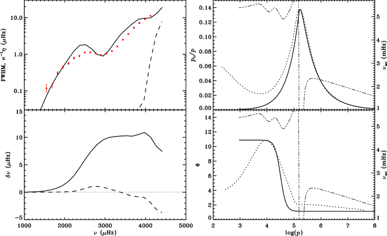
Figure 1: Solar model properties calculated by Houdek et al. (2017), who adopted the nonlocal parameters $a=8.37$, $b=44.72$, $c=4.43$, $\varPhi_{\rm c}=1.13$ for the anisotropy parameter in the deep convective interior, and $Y=0.245$ and $Z=0.018055$ for the helium and heavy-element abundances by mass.. Top left: comparison of BiSON linewidths (symbols with error bars from Chaplin et al., 2005) and $\pi^{-1}\eta$, where $\eta$ is the theoretical damping rate for radial modes; note that $\pi^{-1}\eta$ corresponds to the full width at half maximum, in cyclic frequency, of the peaks in the observed power spectrum. The solid curve is the result of the full calculation in which both the perturbations to the convective heat and momentum fluxes were included. The dashed curve displays the damping rates for a stability calculation in which the perturbation to the momentum flux, $\updelta p_{\rm t}$, was suppressed. Bottom left: modal frequency corrections, $\updelta\nu$, relative to a standard adiabatic frequency calculation in which the Lagrangian perturbation to turbulent pressure vanishes. The solid curve includes both the perturbations to the convective heat and momentum fluxes and the dashed curve is the modal frequency correction for a calculation in which the perturbation to the momentum flux, $\updelta p_{\rm t}$, was suppressed. Top right: comparison of the turbulent pressure profile, $p_{\rm t}/p$, between the 3D simulation (dotted curve; Trampedach et al. 2014b) and the 1D nonlocal solar envelope model (solid curve). Bottom right: comparison of the turbulent velocity anisotropy, $\varPhi$, between the 3D simulation (dotted curve) and the 1D model (solid curve). In the right-hand panels the double-dot-dashed curve is the acoustic cutoff frequency $\nu_{\rm ac}$ (Deubner & Gough, 1984) of the 1D, nonlocal, reference model.

The linear nonadiabatic pulsation calculations are carried out using the same nonlocal convection formulation with the assumption that all eddies in the cascade respond to the pulsation in phase with the dominant large eddies. A simple thermal outer boundary condition is adopted at the temperature minimum where for the mechanical boundary condition the solutions are matched smoothly onto those of a plane-parallel isothermal atmosphere for frequencies below the acoustic cutoff frequency $\nu_{\rm ac}$, i.e. the solutions are matched onto an exponential solution with the energy density decreasing with height in the atmospheres. For modes with frequencies larger than $\nu_{\rm ac}$ the eigenfunctions are matched to an outwardly running wave, allowing for transmission of energy into the atmosphere (e.g., Balmforth & Gough, 1990; Balmforth et al., 2001). At the base of the model envelope ($r/R_{\star}=0.2$) the conditions of adiabaticity and vanishing of the displacement eigenfunction are imposed. Only radial p modes are considered.

In addition to the fully nonadiabatic calculations, which include the modal perturbations to the convective heat and momentum fluxes, we also computed frequencies in the adiabatic approximation for the same equilibrium models. In our adiabatic calculation we assume that the modal Lagrangian perturbation to the turbulent pressure, $\updelta{p_{\mathrm{t}}}$, is in quadrature with the modal density perturbation, $\updelta\rho$. This leads to a modification of the first adiabatic exponent, $\gamma_{1}:=(\partial\ln{p_{\mathrm{g}}}/\partial\ln\rho)_{s}$ (${p_{\mathrm{g}}}$ is gas pressure), in the linearized, adiabatic pulsation equations, i.e. the Lagrangian (total) pressure perturbation, $\updelta\ln p=({p_{\mathrm{g}}}/p)\gamma_{1}\updelta\ln\rho$ (Houdek et al., 2017), also referred to as the reduced $\gamma_{1}$ (Rosenthal et al., 1995). From taking the differences between the fully nonadiabatic, $\nu_{\rm na}$, and adiabatic, $\nu_{\rm a}$, frequencies, we obtain estimates for the modal frequency corrections, $\delta\nu:=\nu_{\rm na}-\nu_{\rm a}$, i.e. the modal contribution to the so-called “surface effects” (e.g., Rosenthal et al., 1999).

5 Results

5.1 The solar benchmark case

We start by reviewing Houdek’s et al. (2017) solar results depicted in Fig. 1. The adopted 1D profile for the velocity-anisotropy parameter $\varPhi$ (solid curve in the lower right panel) is in good agreement with the 3D profile (dotted curve), particularly in the mode-propagating layers ($\log p\geq 5.2$). The regions where the modes are either propagating ($\log p\geq 5.2$) or evanescent ($\log p<5.2$) are indicated by the acoustic cutoff frequency, $\nu_{\rm ac}$ (double-dot-dashed curve). The mode frequencies are predominantly determined by the mode-propagating regions which therefore also affect the modal frequency corrections discussed later in Section 6. The remaining differences in $\varPhi$ with respect to the 3D solution in the mode-propagating layers do, however, affect the solutions of our damping-rate calculations. We note that the effect of $\varPhi$ on mode damping is strongly coupled to the filling factor (fractional area of, e.g., upflows), which is always $1/2$ in any 1D convection model that adopts the Boussinesq approximation (Spiegel & Veronis, 1960) and assumes symmetry between up- and downflows. Therefore, it is not expected that our 1D convection treatment yields the observed damping rates, even if the complete 3D $\varPhi$-profile is adopted in our stability analyses. Only a full 3D hydrodynamical simulation of the full oscillation properties would adequately describe the problem. This is still out of reach as of today. Houdek et al. (2017) therefore found it more useful and relevant to reproduce the observed damping rates by adopting the 1D $\varPhi$-profile as indicated by the solid curve in the lower right panel of Fig. 1 for the Sun. We do adopt the same procedure here for our LEGACY models. Moreover, the inclusion of a depth-dependent $\varPhi$-profile in our 1D pulsation analyses, with a shape and extrema adopted from 3D simulations, and its consistent pulsational perturbation, $\updelta\varPhi$ (the Lagrangian operator $\updelta$ indicates a perturbation following the motion), in the stability analyses, is a novelty in this work. The expression for $\updelta\varPhi$ is given in e.g., Houdek & Dupret (2015, equation 74 and Appendix B). The turbulent pressure, $p_{\rm t}$, on the other hand, is robust to changes in filling factor, since it depends on the unsigned vertical convective velocity, and therefore reproduces the 3D solution very well in the mode-propagating layers. In the outer stellar layers, where the differences in the $p_{\rm t}$-profiles between the 1D and 3D solutions are largest, the contribution of the perturbed turbulent pressure, $\updelta{p_{\mathrm{t}}}$, to the damping rates, $\eta$, is negligible as suggested by an analysis of the associated work integral $W_{\rm t}$ (see, e.g., Balmforth, 1992a; Houdek, 1996). Only at deeper stellar layers with $\log p\gtrsim 5.0$ does the work of $\updelta{p_{\mathrm{t}}}$ start to become relevant with a relative contribution of about 8% to $W_{\rm t}$ for a mode with a frequency close to $\nu_{\rm max}$. At these deeper stellar layers, however, the differences in the $p_{\rm t}$-profiles between the 1D and 3D solutions are already small. Similar results are also observed for our LEGACY models.

The dashed curves in the left panels of Fig. 1 show the (positive) damping rates (top panel) and modal frequency corrections (bottom panel) for a computation in which the pulsationally perturbed turbulent pressure, $\updelta{p_{\mathrm{t}}}$, is artificially suppressed. As expected, only the highest frequency modes are found to be stable, mainly due to the radiative damping of these high-frequency modes, whereas for frequencies less than about 3.8 mHz the pulsation modes are predicted to be unstable in this case (see also e.g. Houdek et al., 1999).

Modal frequency corrections for a computation in which $\updelta{p_{\mathrm{t}}}$ is artificially suppressed (dashed curve in bottom left panel) indicate that nonadiabatic effects from the pulsationally perturbed radiative and convective heat fluxes are rather minute, i.e. most of the modal frequency corrections as indicated by the solid curve in the bottom left panel is due to the effects of convection dynamics associated with $\updelta{p_{\mathrm{t}}}$. We should, however, remain aware that due to the nonlinear nature of the convection-pulsation interaction, the individual contributions to the modal surface effects cannot simply be explained by linear superposition, e.g., by simply taking the differences between the solid and dashed curves in the left panels of Fig. 1.

5.2 Effects of varying model parameters

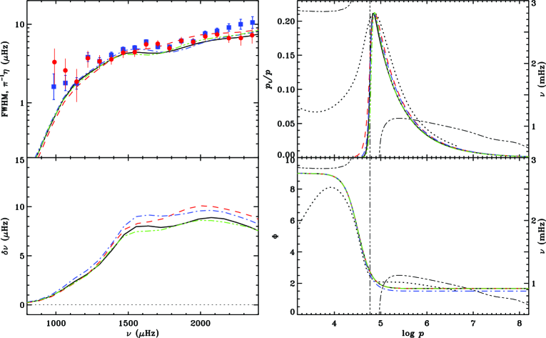
Figure 2: Model properties of KIC 9139163. Results are shown for four different models with only one model parameter being different in each model calculation: the solid, black, curves are the results for the model parameters listed in Table 1, i.e. the reference model; the dashed, red, curves are the results for a model computation in which the depth of the surface convection zone is increased by 5%, relatively to the ASTEC model; the dot-dashed, blue, curves assume, in the deep convection layers, the smaller velocity-anisotropy parameter $\varPhi_{\rm c}=3/2$, relatively to the reference value $\varPhi_{\rm c}=5/3$; the double-dot-dashed, green, curves adopt the heavy-element abundance by mass of the 3D grid, $Z=0.018055$, and helium abundance by mass, $Y=0.245$. Top left: comparison of observed linewidths (red solid circles with error bars are the LEGACY data from Lund et al. 2017, blue filled squares with error bars are from Appourchaux et al. 2014, 2016) and $\pi^{-1}\eta$ (curves). Bottom left: radial modal frequency corrections $\updelta\nu$ relative to a standard adiabatic pulsation calculation. Top right: comparison of the turbulent pressure profile $p_{\rm t}/p$ between 3D simulation (dotted curve; Trampedach et al. 2014a) and the four 1D nonlocal stellar envelope models (remaining curves). Bottom right: comparison of the turbulent velocity anisotropy $\varPhi$ between 3D simulation (dotted curve) and 1D models (remaining curves). The acouctic cutoff frequency, $\nu_{\rm ac}$, of the reference model is indicated by the double-dot-dashed, black, curves in the right panels. See also caption to Fig. 1.

The effect of varying the nonlocal parameters $a$, $b$ and $c$ on the estimated damping rates were presented in detail by Balmforth (1992a) for the solar case and recently by Aarslev et al. (2018) for red-giant stars. We therefore only summarize their effects here for the LEGACY stars, but discuss additionally the effects of varying the depth of the surface convection zone, $d_{\rm c}$, velocity anisotropy, $\varPhi_{\rm c}$, and heavy-element abundance $Z$, on our results for the LEGACY star KIC 9139163, depicted in Fig. 2.

The best-constrained nonlocal convection parameter is $c$, which controls the degree of “nonlocality” of the turbulent pressure, ${p_{\mathrm{t}}}$, i.e. the spatial coherence of the ensemble of eddies contributing to the turbulent momentum flux. We calibrate $c$ by making the maximum value of ${p_{\mathrm{t}}}$ in the superadiabatic boundary layer of the 1D solution of our reference model (solid curve in the upper right panel of Fig. 2) agree with the value obtained from the 3D simulation result (dotted curve in the upper right panel). The stellar depth at which these maxima occur agree well between the 1D and 3D solutions without any further calibration, provided the heavy-element abundance is similar between the 1D and 3D models (see double-dot-dashed, green, curve in upper right panel, and discussion below). Similarly to $c$, the role of the nonlocal parameter $a$ is to control the spatial coherence of the ensemble of eddies contributing to the convective heat (enthalpy) flux. This parameter cannot be constrained in a straightforward manner by the 3D simulation, because the adopted nonlocal convection model does not provide the correct enthalpy flux in the overshoot regions. Instead we calibrate the nonlocal parameter $a$ so as to obtain a good agreement between observed linewidths and computed damping rates (upper left panel of Fig. 2). Larger values of $a$ result in a less pronounced depression in the damping rates, $\eta$, near $\nu_{\rm max}\simeq 1730\,\mu$Hz (see also Aarslev et al. 2018). The third nonlocal convection parameter $b$ controls the degree to which the turbulent fluxes are coupled to the local stratification. The larger the value of $b$ the stronger the turbulent fluxes are coupled to the local stratification, resulting in less drastic changes in the stratification such as the superadiabatic temperature gradient (see also Balmforth 1992a and Aarslev et al. 2018). Similarly to $a$, changes to the value of $b$ affects predominantly the amount of the depression in the damping rate, $\eta$, near $\nu_{\rm max}$, leading to some degeneracy between $a$ and $b$, and consequently to a correlation between the results of calibrating $a$ and $b$ to the observed linewidths. A possible remedy could include a more extensive use of 3D simulations by calibrating $b$ to the superadiabatic temperature gradient of 3D simulation results thereby breaking the degeneracy between $a$ and $b$, which we plan in a future effort to improve the convection model.

In Fig. 2 we show for KIC 9139163 the effect of reducing the velocity-anisotropy parameter, $\varPhi_{\rm c}$ in the deep convection zone (lower right panel) from $\varPhi_{\rm c}=5/3$ (solid, black, curve; overplotted by identical dashed, red, and double-dot-dashed, green, curves) to $\varPhi_{\rm c}=3/2$ (dot-dashed, blue, curve) keeping, however, the other model properties constant, including the depth of the convection zone, $d_{\rm c}$, $\max({p_{\mathrm{t}}})$ and $\varPhi_{\rm s}$. The corresponding results in the other panels are also depicted by dot-dashed, blue, curves and should be compared with the reference solutions illustrated by the solid, black, curves. There is rather little effect on the turbulent pressure profile (upper right panel) but noticeable effect on the damping rates (upper left panel) and modal surface correction (lower left panel). Reducing $\varPhi_{\rm c}$ decreases the characteristic timescale of the convection and consequently increases the frequency at which energy is exchanged most effectively between convection and pulsation. This is demonstrated in the upper left panel of Fig. 2 by the increased frequency at which the minimum in the depression of the damping rates is observed (dot-dashed, blue, curve). Varying the value of $\varPhi_{\rm s}$ has comparatively little effect on $\eta$ and the surface corrections (not shown here). Also, different 3D simulation codes predict different values for $\varPhi_{\rm s}$ (F. Kupka, personal communication, see also Kupka & Muthsam 2017), possibly because of different surface boundary conditions in the various 3D simulation codes.

The effect of increasing the depth of the convection zone, $d_{\rm c}$, by 5%, relatively to the ASTEC evolutionary model, is illustrated by the dashed, red, curves in Fig. 2. The results should be compared with the reference model (solid, black, curves). There is a slightly better agreement of the ${p_{\mathrm{t}}}$-profile with the 3D solution (dotted, black, curve), depicted in the upper right panel. The damping-rate increase with $d_{\rm c}$ (upper left panel), however, is substantial, as is the increase of the modal frequency correction (lower left panel). A deeper surface convection zone requires a smaller value for the calibrated nonlocal convection parameter $c$, explaining in part the better agreement of the ${p_{\mathrm{t}}}$-profile with the 3D simulation results, as a result of a slower exponential decay of ${p_{\mathrm{t}}}$ in the overshoot regions.

The double-dot-dashed, green, curves in Fig. 2 show the outcome for a computation in which the heavy-element abundance was reduced from the reference value $Z=0.0295$, as determined from the LEGACY model fitting to the observed Kepler frequencies (see Table 1), to the value $Z=0.018055$ (and $Y=0.245$), adopted by the 3D simulation grid (see Section 3). The comparison with the more metal-rich reference model (solid, black, curves) should demonstrate the effect of our inconsistent use of heavy-element abundance between our calibrated 1D stability computation and the 3D simulation grid. Although the effect of this inconsistency in $Z$ fortunately appears to be minute on $\eta$ and on the modal surface corrections, it is our aim to recalibrate, in a future effort, consistently our 1D models with 3D simulations of the appropriate composition, once such a 3D grid for a range of metallicities will be available.

5.3 Damping rates and modal surface effects

The model results were obtained from calibrating the free convection parameters, $a$, $b$, $c$, $\varPhi_{\rm s}$ and $\varPhi_{\rm c}$, together with the mixing-length parameter $\alpha$, in a similar manner as discussed by Aarslev et al. (2018). The parameters $c$, $\varPhi_{\rm s}$ and $\alpha$ are calibrated first, by iteration, to match the profiles of the 3D simulations for turbulent pressure, ${p_{\mathrm{t}}}/p$, and anisotropy, $\varPhi$, in the mode-propagating layers, and to the surface convection-zone depths, $d_{\rm c}$, of the ASTFIT models. The remaining parameters, $a$, $b$ and $\varPhi_{\rm c}$ are then determined by obtaining the best agreement between theoretical damping rates and observed linewidths. The parameter $\varPhi_{\rm c}$ predominantly affects the frequency of the depression in the damping rates, $\eta$, typically near $\nu_{\rm max}$, whereas the nonlocal parameter $a$ predominantly affects the depth of this depression in $\eta$. Finally, the parameter $b$ is calibrated by iteration, to reproduce the observed linewidths as well as possible at low and high frequencies (see also, Aarslev et al., 2018). Owing to the rather low sensitivity of $\eta$ to the parameter $b$, the value of $b$ resulting from this fit is somewhat uncertain.

The quality of the observed linewidths does not support a full statistical analysis, including a formal $\chi^{2}$ minimization. Moreover, the differences between theoretical damping rates and observed linewidths are still dominated by systematics brought about by our still poor understanding of modelling the convection-pulsation physics (see, for example, top left panel in Fig. 1 for the solar case). The aim of the procedure for finding the optimal model, as outlined above, is therefore to find the best qualitative agreement with the 3D simulation results and linewidth measurements. In this fitting procedure we have, however, evaluated $\chi^{2}$ between observed linewidths and damping rates for several of the parameter choices, and the parameter values listed in Table 1 do correspond to the fit with the lowest $\chi^{2}$ amongst the parameter sets considered. This lowest $\chi^{2}$ between linewidths and damping rates over the full observed frequency range is listed in Table 2. Moreover, in addition to fitting the linewidths, our 1D models also aim to simultaneously reproduce the turbulent pressure and anisotropy profiles of 3D simulations in the mode-propagating layers and the surface convection-zone depths, $d_{\rm c}$, of the ASTFIT models.

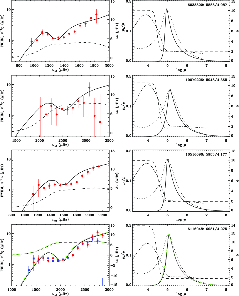
Figure 6: LEGACY model results. The KIC numbers and surface values, $T_{\rm eff}(K)\,$/$\,\log\mathcmr{g}$, of the LEGACY stars are indicated in the right panels. Plots are arranged in order of increasing $T_{\rm eff}$ from top to bottom. Left: comparison between observed linewidths (FWHM, red solid circles with error bars are the LEGACY data from Lund et al. 2017, blue filled squares with error bars are from Appourchaux et al. 2014, 2016) and $\pi^{-1}\eta$ (see caption to Fig. 1). The dashed curves are the radial modal frequency corrections, $\updelta\nu$, relative to a standard adiabatic pulsation calculation. Right: comparison of the turbulent pressure profile $p_{\rm t}/p$ between 3D simulations (dotted curves; Trampedach et al. 2014a) and 1D nonlocal envelope model (solid curves). The dot-dashed curves are the turbulent velocity anisotropies $\varPhi$ of 3D simulations and the dashed curves the adopted depth-dependent velocity anisotropies in the 1D models. The double-dot-dashed, green curves for KIC 6116048 adopt the 3D-grid abundances, $Z=0.018055$ and $Y=0.245$.

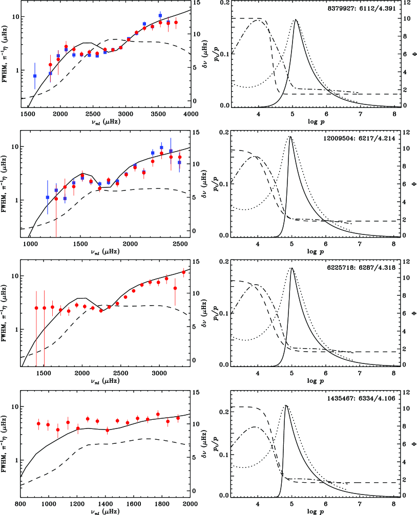
Figure 7: LEGACY model results. Details are as in the caption of Fig. 6.

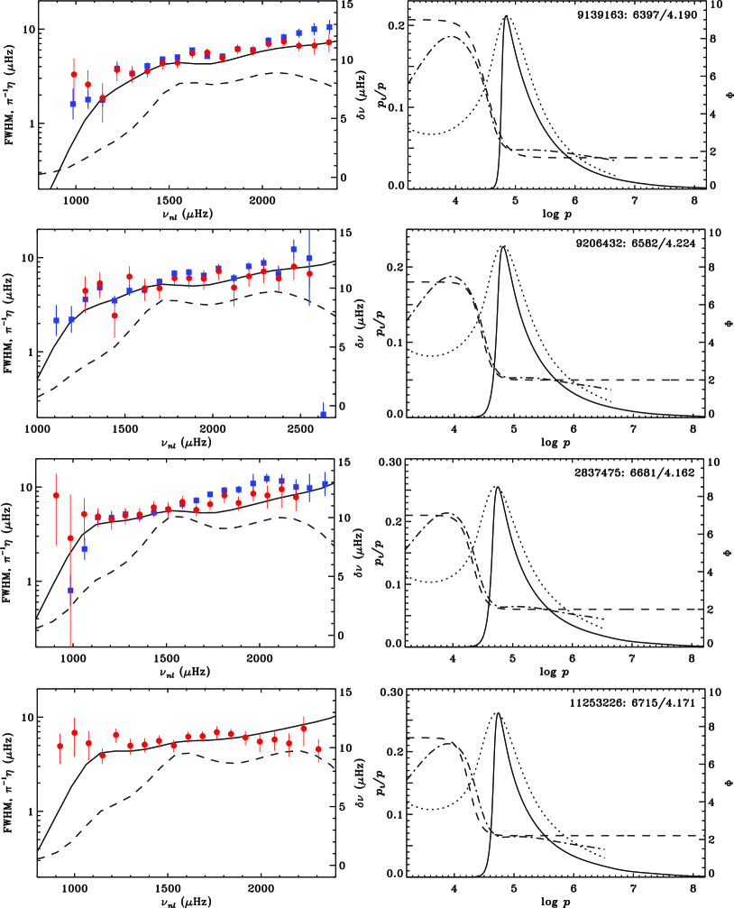
Figure 8: LEGACY model results. Details are as in the caption of Fig. 6.

Detailed results for our sample of twelve LEGACY stars, listed in Table 1, are illustrated in Figs 6–8. The left panels compare observed linewidths (symbols with error bars), which correspond to the full width at half maximum (FWHM) of the spectral peaks in the observed power spectrum, with our calculated values of $\pi^{-1}\eta$ (solid curves, see caption of Fig.1) as a function of pulsation frequency. Also shown are the modal frequency corrections (dashed curve) relative to a standard adiabatic oscillation calculation for the same equilibrium model, following the procedure by Houdek et al. (2017). The right panels in Figs 6–8 compare turbulent pressure profiles, $p_{\rm t}/p$, and velocity anisotropies, $\varPhi$, between our 1D equilibrium models (solid and dashed curves, respectively) and 3D simulations (dotted and dot-dashed curves, respectively). There is good agreement between the 3D-simulation results and calibrated 1D-equilibrium models in the mode-propagating layers and, at the same time, also between the observed linewidths and estimated values of $\pi^{-1}\eta$, for all considered LEGACY models. As in the solar case (Fig. 1) the stellar depths of the maxima of $p_{\rm t}/p$ in the 1D and 3D results agree fairly well, except for models for which the heavy-element abundance $Z$ differs considerably between our 1D computations and the 3D simulations, such as for the stellar models KIC 6116048 and KIC 9139163. The effect of adopting the chemical abundances of the 3D simulations (see Section 3) on the 1D-profiles of $p_{\rm t}/p$ are indicated by the double-dot-dashed, green curves in Fig. 2 for KIC 9139163, and in Fig. 6 (bottom panels) for KIC 6116048. For KIC 6116048 and KIC 1435467 we adopt slightly larger values for $\varPhi_{\rm s}$, compared with the 3D results, leading to better agreement between linewidth measurements and theoretical damping rates, though the effect of varying $\varPhi_{\rm s}$ on $\pi^{-1}\eta$ is rather small. Moreover, as discussed also in Section 5.2, various 3D hydrodynamical simulation codes predict noticeable differences for $\varPhi_{\rm s}$.

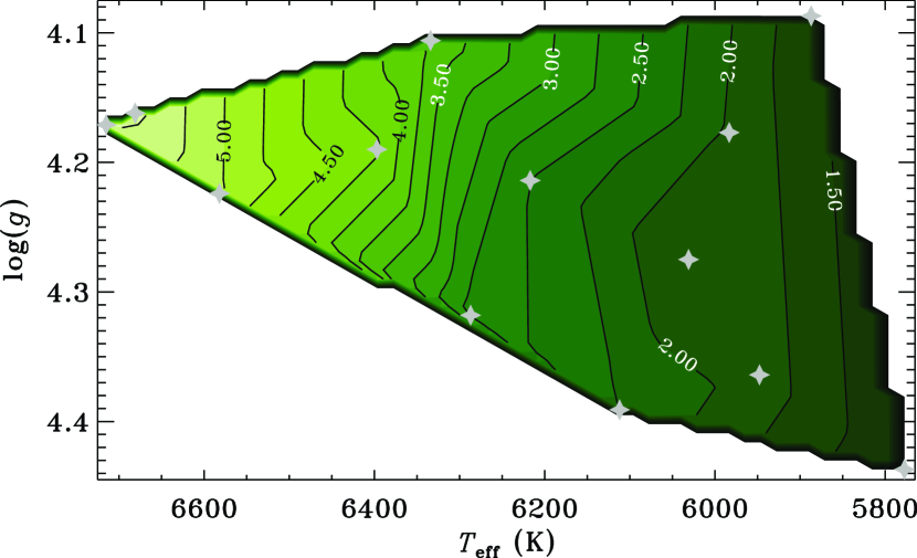
Figure 3: Modelled $\pi^{-1}\eta$, where $\eta$ is the damping rate, corresponding to the full width at half maximum (FWHM) of the spectral peaks in the power spectrum. Results, in units of $\mu$Hz, are plotted as contours in a Kiel diagram at the observed frequency of maximum pulsation power, $\nu_{\rm max}$ (see Table 2). The star symbols indicate the locations of the twelve selected LEGACY stars and the Sun.

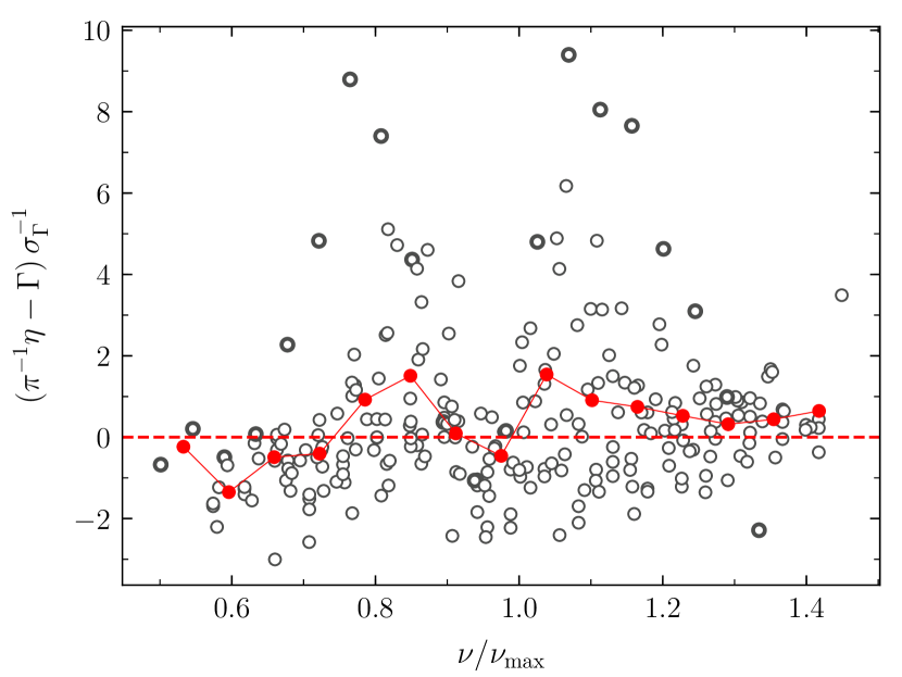
Figure 4: Residuals between modelled $\pi^{-1}\eta$, where $\eta$ is the damping rate, and observed linewidths, $\Gamma$, as a function of the $\nu_{\rm max}$-normalized mode frequencies, $\nu/\nu_{\rm max}$, for all twelve LEGACY stars. The residuals have further been normalized by the uncertainty of the observed linewidths. Each open circle corresponds to the value of a given pulsation mode. Red solid circles (connected) are uniformly weighted mean values of the individual mode values in 0.06 wide bins. The thick-edge open circles show the values for the Sun using BiSON mode linewidths.

Table 2: Solar and LEGACY model results at the frequency of maximum oscillation power, $\nu_{\rm max}$. The first three columns are the Kepler Input Catalog (KIC) number, observed $\nu_{\rm max}$, and modal frequency corrections, $\delta\nu$. The next two columns list the observed linewidths, $\Gamma$, and modelled $\pi^{-1}\eta$ at $\nu_{\rm max}$. $\Gamma(\nu_{\rm max})$ was determined from fitting to the data the analytical expression (1) by Appourchaux et al. (2016), and $\pi^{-1}\eta(\nu_{\rm max})$ was obtained from linear interpolation in the modelled estimates $\eta(\nu)$. The last two columns show the reduced $\chi^{2}$ values between the observed, $\Gamma$, and modelled, $\pi^{-1}\eta$, data, calculated as $\chi^{2}_{r}=({N-2})^{-1}\sum_{i=1}^{N}\sum_{j=1}^{N}(\Gamma_{i}-\pi^{-1}\eta_{i})\,C^{-1}_{ij}\,(\Gamma_{j}-\pi^{-1}\eta_{j})$, where ${\bf C}$ is the covariance matrix for $\Gamma$, and $N$ represents the number of fitted linewidths. Solar observations are from BiSON (Chaplin et al., 2005) and solar model results from Houdek et al. (2017). For the BiSON linewidths we adopted a diagonal covariance matrix.

KIC	$\nu_{\rm max}\ (\mu$Hz)	$\delta\nu\ (\mu$Hz)	$\Gamma\ (\mu$Hz)	$\pi^{-1}\eta\ (\mu$Hz)	$\chi^{2}$	$N$
Sun	3090	10.0	1.06$\,\pm\,$0.03	1.25	25.20	20
6933899	1390	3.7	1.30$\,\pm\,$0.07	1.56	10.92	13
10079226	2653	7.4	2.05$\,\pm\,$0.35	1.89	3.81	12
10516096	1690	4.6	1.56$\,\pm\,$0.10	1.97	12.33	13
6116048	2127	6.2	1.62$\,\pm\,$0.09	1.73	17.74	15
8379927	2795	9.2	2.43$\,\pm\,$0.11	2.25	11.38	17
12009504	1866	5.9	2.38$\,\pm\,$0.14	2.49	4.98	15
6225718	2364	8.1	2.58$\,\pm\,$0.12	2.66	7.37	19
1435467	1407	7.0	5.18$\,\pm\,$0.17	3.70	4.13	15
9139163	1730	7.9	5.28$\,\pm\,$0.13	4.30	3.41	19
9206432	1866	8.7	5.87$\,\pm\,$0.27	5.02	1.90	16
2837475	1558	10.1	6.39$\,\pm\,$0.20	5.57	1.91	18
11253226	1591	9.5	5.80$\,\pm\,$0.17	5.53	5.26	19

Values of the LEGACY linewidths, $\Gamma$, and computed $\pi^{-1}\eta$ are listed in Table 2 at the frequency of maximum oscillation power, $\nu_{\rm max}$, together with our modal frequency corrections, $\delta\nu(\nu_{\rm max})$. The values for $\Gamma$ are obtained from fitting Appourchaux’s et al. (2016) expression (1) to the observed linewidths, following the procedure by Lund et al. (2017), and the $\pi^{-1}\eta$ values are obtained from interpolating in the frequency-dependent damping rates.

As reported before (Chaplin et al., 2009; Belkacem et al., 2012), the increase of the observed linewidths with increasing surface temperature, $T_{\rm eff}$, is also reproduced here with our stability analysis, as illustrated in Fig. 3. There is also a dependence on surface gravity (see also Houdek, 2017), but of much smaller magnitude. Moreover, the decrease of the amount of the depression in the linewidths near $\nu_{\rm max}$ with increasing $T_{\rm eff}$, as reported previously by Appourchaux et al. (2014) and Lund et al. (2017), is also reproduced by our theoretical damping rates (see Figs 6–8).

Fig. 4 shows the residuals between observed linewidths and estimated $\pi^{-1}\eta$ for all fitted modes, divided by the measurement uncertainties, and on a frequency scale normalized by $\nu_{\rm max}$. There is still a discrepancy between observations and models just below and above $\nu_{\rm max}$, as can also be seen for the solar case (upper left panel of Fig. 1). This discrepancy is predominantly a consequence of the still incompletely modelled superadiabatic boundary layers. The thermal relaxation time of the superadiabatic boundary layer, when expressed as a frequency, $\nu_{\rm p}$, is of similar order as the frequency at which the depression in the linewidths is observed ($\nu_{\rm p}\simeq$ 2.8 mHz in the solar case, the exact value depending upon the nonlocal convection parameters; Balmforth 1992a, Chaplin et al. 2005). It is at this frequency $\nu_{\rm p}$ where the energy exchange between the pulsation and the stellar background is most efficient (e.g., Houdek & Dupret, 2015). Any insufficient representation of either the stellar mean stratification or the thermal and dynamical properties of the superadiabatic boundary layers are revealed by a mismatch between the modelled damping rates and linewidth measurements. In a future investigation we plan to identify the reason for this mismatch by comparing the properties of the superadiabatic boundary layer with 3D simulation results. It is interesting to note that a more careful calibration of the nonlocal convection parameter $b$ (see Section 4) with the help of 3D simulation results, together with an analysis of work integrals, could identify possible missing physics in our model calculations, such as the effect of kinetic energy transport (e.g., Gough, 2012).

In Fig. 5 the modal frequency corrections, $\delta\nu$, at $\nu_{\rm max}$, also listed in Table 2, are plotted as contours in a Kiel diagram. The top panel shows $\delta\nu$ in $\mu$Hz, whereas the bottom panel displays the relative modal correction, $\delta\nu/\nu_{\rm max}$, in order to show the relative importance of the modal frequency shift with respect to mode frequency. There is a clear trend with stellar surface values, particularly the increase of $\delta\nu/\nu_{\rm max}$ with surface temperature.

6 Discussion and conclusions

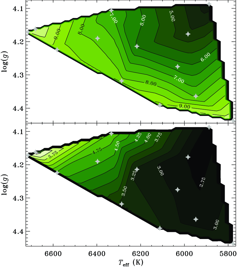
Figure 5: Modal frequency corrections, $\updelta\nu$, relative to a standard adiabatic pulsation calculation. Results are plotted as contours in a Kiel diagram at the observed frequency, $\nu_{\rm max}$ (see Table 2), of maximum pulsation power. Top: the contours are labelled in units of $\mu$Hz. Bottom: contours show $(\updelta\nu/\nu_{\rm max})\times 10^{3}$ in order to illustrate the relative modal frequency shift with respect to mode frequency. The star symbols indicate the locations of the twelve selected LEGACY stars and the Sun.

It has been the aim of this paper to demonstrate the simultaneous modelling of observed and 3D-simulated stellar properties in main-sequence stars that are typically not included in standard stellar evolutionary calculations. In particular, we included in our 1D stellar models turbulent pressure and velocity-anisotropy profiles as suggested by realistic 3D simulations of convective stellar atmospheres, and, at the same time, obtained good agreement between pulsation-linewidth measurements and modelled damping rates over the full observed frequency range. The remaining differences, e.g., in the ${p_{\mathrm{t}}}/p$-profiles between 1D and 3D models in the deeper, mode-propagating layers, help us to assess missing physics, such as the kinetic energy flux (e.g., Gough, 2012), convective backwarming (e.g., Trampedach et al., 2017) and the asymmetry between up- and downflows, that is required for further improving our current 1D models for convective energy transport.

It is interesting to note that models with deeper surface convection zones, compared with the ASTFIT models (see Section 2), reproduce the observed pulsation-linewidth profiles somewhat better, particularly for the hotter stars in our LEGACY stellar sample (see for example Fig. 2). This is a result of the increasing damping rates with increasing mixing length, mostly due to the contributions from the turbulent pressure perturbations. This effect may therefore serve as an additional constraint for calibrating convection in stellar models and the consequent extent of surface convection zones. Other procedures to constrain surface convection-zone depths include the use of acoustic glitches (e.g., Gough, 1990). This method, however, needs very accurate pulsation frequencies, and current glitch models are still affected by the poorly understood glitch contribution from hydrogen ionization and the difficult-to-determine location of the star’s acoustic surface (e.g., Houdek & Gough, 2007; Mazumdar et al., 2014; Reese et al., 2016).

Another interesting outcome of our stability analyses is the prediction of the modal frequency contribution to the so-called ‘surface effects’. By combining our modal frequency corrections, $\delta\nu$, relative to a standard adiabatic pulsation calculation, with structural, adiabatic, frequency corrections, $\delta\nu^{\rm s}$ (e.g., Trampedach et al., 2017), we would have, for the first time, a purely physical description for the total surface frequency corrections, $\Delta\nu:=\delta\nu+\delta\nu^{\rm s}$, at hand. For a calibrated solar model, Houdek et al. (2017) obtained at the frequency of maximum oscillation power, $\nu_{\rm max}\simeq 3090\,\mu$Hz, the values $\delta\nu\simeq 10.0\,\mu$Hz and $\delta\nu^{\rm s}\simeq-16.0\,\mu$Hz, leading to an underestimation (i.e. over-correction) of the fully surface-corrected model frequency of $\sim 1.4\,\mu$Hz, relative to the observed solar frequency (see fig. 5 of Houdek et al. 2017). We have, however, to remain aware how stellar-model fits to seismic observations, such as the ASTFIT models (Section 2), exhibit coupled parameters. In particular the surface effect, mixing length (e.g., Li et al. 2018) and helium abundance can be strongly correlated, stressing the importance of constraining these quantities independently. Moreover, $\delta\nu$ also depends on metallicity as demonstrated in Fig. 2 for KIC 9139163. We therefore plan to address these open issues in future work by exploiting additional information from 3D simulation results in a fully consistent way, such as adopting the 3D atmosphere structures (Trampedach et al., 2014a) and 3D-simulation-calibrated mixing lengths (Trampedach et al., 2014b) in the ASTFIT models (Section 2). Also, a necessary step will be the implementation of a pipeline that will take into account a full statistical analysis of the measured linewidth errors and a consistent treatment of frequency corrections, based on our theoretical formulation involving a physical model, in both the ASTFIT and pulsation-stability calculations.

We have demonstrated that the additional stellar properties, considered in this work, further constrain the theory of stellar structure and evolution. The combined effort of improving the modelling in this manner and extending the analysis to a broader range of observed stars will, one may hope, improve our understanding of the properties of stellar convection and its interaction with pulsations. Such improvements in the modelling of the near-surface layers are also crucial for reducing their effect on the computed frequencies and consequently improving the characterization of stellar properties through frequency fitting.

Appendix A Detailed results for all twelve calibrated LEGACY models

In this appendix we plot the frequency-dependent damping rates and modal surface corrections for our sample of twelve LEGACY stars (see Table 1), together with the calibrated 1D and 3D solutions of the turbulent pressure profiles, ${p_{\mathrm{t}}}$, and velocity anisotropies, $\varPhi$.

References

- Aarslev et al. (2018) Aarslev M. J., Houdek G., Handberg R., Christensen-Dalsgaard J., 2018, MNRAS, 478, 69
- Angulo et al. (1999) Angulo C., et al., 1999, Nuclear Physics A, 656, 3
- Appourchaux et al. (2014) Appourchaux T., et al., 2014, A&A, 566, A20
- Appourchaux et al. (2016) Appourchaux T., et al., 2016, A&A, 595, C2
- Baglin et al. (2009) Baglin A., Auvergne M., Barge P., Deleuil M., Michel E., CoRoT Exoplanet Science Team 2009, in Pont F., Sasselov D., Holman M. J., eds, IAU Symposium Vol. 253, IAU Symposium. International Astronomical Union, Cambridge, pp 71–81, doi:10.1017/S1743921308026252
- Baker & Gough (1979) Baker N. H., Gough D. O., 1979, ApJ, 234, 232
- Ball et al. (2016) Ball W. H., Beeck B., Cameron R. H., Gizon L., 2016, A&A, 592, A159
- Balmforth (1992a) Balmforth N. J., 1992a, MNRAS, 255, 603
- Balmforth (1992b) Balmforth N. J., 1992b, MNRAS, 255, 632
- Balmforth & Gough (1990) Balmforth N. J., Gough D. O., 1990, ApJ, 362, 256
- Balmforth et al. (2001) Balmforth N. J., Cunha M. S., Dolez N., Gough D. O., Vauclair S., 2001, MNRAS, 323, 362
- Belkacem et al. (2012) Belkacem K., Dupret M. A., Baudin F., Appourchaux T., Marques J. P., Samadi R., 2012, A&A, 540, L7
- Böhm-Vitense (1958) Böhm-Vitense E., 1958, Zeitschrift für Astrophysik, 46, 108
- Borucki (2016) Borucki W. J., 2016, Rep. Prog. Phys., 79, 036901
- Borucki et al. (2010) Borucki W. J., et al., 2010, Science, 327, 977
- Brown (1984) Brown T. M., 1984, Science, 226, 687
- Chaplin et al. (2005) Chaplin W. J., Houdek G., Elsworth Y., Gough D. O., Isaak G. R., New R., 2005, MNRAS, 360, 859
- Chaplin et al. (2009) Chaplin W. J., Houdek G., Karoff C., Elsworth Y., New R., 2009, A&A, 500, L21
- Christensen-Dalsgaard (1982) Christensen-Dalsgaard J., 1982, MNRAS, 199, 735
- Christensen-Dalsgaard (2008a) Christensen-Dalsgaard J., 2008a, Ap&SS, 316, 13
- Christensen-Dalsgaard (2008b) Christensen-Dalsgaard J., 2008b, Ap&SS, 316, 113
- Christensen-Dalsgaard (2012) Christensen-Dalsgaard J., 2012, Astronomische Nachrichten, 333, 914
- Christensen-Dalsgaard et al. (1989) Christensen-Dalsgaard J., Gough D. O., Libbrecht K. G., 1989, ApJ, 341, L103
- Christensen-Dalsgaard et al. (1996) Christensen-Dalsgaard J., et al., 1996, Science, 272, 1286
- Christensen-Dalsgaard et al. (2009) Christensen-Dalsgaard J., Arentoft T., Brown T. M., Gilliland R. L., Kjeldsen H., Borucki W. J., Koch D., 2009, Communications in Asteroseismology, 158, 328
- Deubner & Gough (1984) Deubner F.-L., Gough D., 1984, ARA&A, 22, 593
- Dupret et al. (2006) Dupret M. A., Barban C., Goupil M.-J., Samadi R., Grigahcène A., Gabriel M., 2006, in Fletcher K., ed., ESA Special Publication Vol. SP-624, Proceedings of SOHO 18/GONG 2006/HELAS I, Beyond the spherical Sun. ESA, Noordwijk, p. 97
- Dupret et al. (2009) Dupret M.-A., et al., 2009, A&A, 506, 57
- Foreman-Mackey et al. (2013) Foreman-Mackey D., Hogg D. W., Lang D., Goodman J., 2013, PASP, 125, 306
- Gilliland et al. (2013) Gilliland R. L., et al., 2013, ApJ, 766, 40
- Goldreich & Keeley (1977) Goldreich P., Keeley D. A., 1977, ApJ, 211, 934
- Gough (1977a) Gough D. O., 1977a, in Spiegel E. A., Zahn J.-P., eds, Lecture Notes in Physics Vol. 71, Problems of Stellar Convection. Springer, Heidelberg, pp 15–56, doi:10.1007/3-540-08532-7_31
- Gough (1977b) Gough D. O., 1977b, ApJ, 214, 196
- Gough (1980) Gough D. O., 1980, in Hill H. A., Dziembowski W. A., eds, Lecture Notes in Physics Vol. 125, Nonradial and Nonlinear Stellar Pulsation. Springer Verlag, Berlin Heidelberg, pp 273–299, doi:10.1007/3-540-09994-8_27
- Gough (1984) Gough D. O., 1984, Advances in Space Research, 4, 85
- Gough (1990) Gough D. O., 1990, in Osaki Y., Shibahashi H., eds, Lecture Notes in Physics, Berlin Springer Verlag Vol. 367, Progress of Seismology of the Sun and Stars. p. 283, doi:10.1007/3-540-53091-6
- Gough (2012) Gough D. O., 2012, ISRN Astronomy and Astrophysics, 2012
- Gough & Weiss (1976) Gough D. O., Weiss N. O., 1976, MNRAS, 176, 589
- Grevesse & Noels (1993) Grevesse N., Noels A., 1993, in Prantzos N., Vangioni-Flam E., Casse M., eds, Origin and Evolution of the Elements. pp 15–25
- Grigahcène et al. (2005) Grigahcène A., Dupret M.-A., Gabriel M., Garrido R., Scuflaire R., 2005, A&A, 434, 1055
- Grigahcène et al. (2012) Grigahcène A., Dupret M.-A., Sousa S. G., Monteiro M. J. P. F. G., Garrido R., Scuflaire R., Gabriel M., 2012, MNRAS, 422, L43
- Grosjean et al. (2014) Grosjean M., Dupret M.-A., Belkacem K., Montalbán J., Samadi R., 2014, in Guzik J. A., Chaplin W. J., Handler G., Pigulski A., eds, IAU Symposium Vol. 301, IAU Symposium. International Astronomical Union, Cambridge, pp 341–344, doi:10.1017/S1743921313014555
- Houdek (1996) Houdek G., 1996, PhD thesis, Formal- und Naturwisseschaftliche Fakultät der Universität Wien
- Houdek (2010) Houdek G., 2010, Astronomische Nachrichten, 331, 998
- Houdek (2017) Houdek G., 2017, in European Physical Journal Web of Conferences. p. 02003 (arXiv:1702.04251), doi:10.1051/epjconf/201716002003
- Houdek & Dupret (2015) Houdek G., Dupret M.-A., 2015, Living Rev. in Solar Phys., 12
- Houdek & Gough (2002) Houdek G., Gough D. O., 2002, MNRAS, 336, L65
- Houdek & Gough (2007) Houdek G., Gough D. O., 2007, MNRAS, 375, 861
- Houdek et al. (1999) Houdek G., Balmforth N. J., Christensen-Dalsgaard J., Gough D. O., 1999, A&A, 351, 582
- Houdek et al. (2017) Houdek G., Trampedach R., Aarslev M. J., Christensen-Dalsgaard J., 2017, MNRAS, 464, L124
- Iglesias & Rogers (1996) Iglesias C. A., Rogers F. J., 1996, ApJ, 464, 943
- Imbriani et al. (2005) Imbriani G., et al., 2005, European Physical Journal A, 25, 455
- Jørgensen et al. (2018) Jørgensen A. C. S., Mosumgaard J. R., Weiss A., Silva Aguirre V., Christensen-Dalsgaard J., 2018, MNRAS, 481, L35
- Kupka & Muthsam (2017) Kupka F., Muthsam H. J., 2017, Living Reviews in Computational Astrophysics, 3, 1
- Kupka et al. (2018) Kupka F., Zaussinger F., Montgomery M. H., 2018, MNRAS, 474, 4660
- Kurucz (1991) Kurucz R. L., 1991, in Crivellari L., Hubeny I., Hummer D. G., eds, NATO Series C Vol. 341, NATO (ASI). p. 441
- Li et al. (2018) Li T., Bedding T. R., Huber D., Ball W. H., Stello D., Murphy S. J., Bland-Hawthorn J., 2018, MNRAS, 475, 981
- Ludwig & Steffen (2016) Ludwig H.-G., Steffen M., 2016, Astronomische Nachrichten, 337, 844
- Ludwig et al. (1999) Ludwig H.-G., Freytag B., Steffen M., 1999, A&A, 346, 111
- Lund et al. (2017) Lund M. N., et al., 2017, ApJ, 835, 172
- Magic & Weiss (2016) Magic Z., Weiss A., 2016, A&A, 592, A24
- Magic et al. (2013) Magic Z., Collet R., Asplund M., Trampedach R., Hayek W., Chiavassa A., Stein R. F., Nordlund Å., 2013, A&A, 557, A26
- Magic et al. (2015) Magic Z., Weiss A., Asplund M., 2015, A&A, 573, A89
- Mazumdar et al. (2014) Mazumdar A., et al., 2014, ApJ, 782, 18
- Michaud & Proffitt (1993) Michaud G., Proffitt C. R., 1993, in Weiss W. W., Baglin A., eds, Astronomical Society of the Pacific Conference Series Vol. 40, IAU Colloq. 137: Inside the Stars. pp 246–259
- Mihalas et al. (1988) Mihalas D., Dappen W., Hummer D. G., 1988, ApJ, 331, 815
- Mosumgaard et al. (2018) Mosumgaard J. R., Ball W. H., Silva Aguirre V., Weiss A., Christensen-Dalsgaard J., 2018, MNRAS, 478, 5650
- Nordlund (1982) Nordlund Å., 1982, A&A, 107, 1
- Piau et al. (2014) Piau L., Collet R., Stein R. F., Trampedach R., Morel P., Turck-Chièze S., 2014, MNRAS, 437, 164
- Reese et al. (2016) Reese D. R., et al., 2016, A&A, 592, A14
- Rogers & Nayfonov (2002) Rogers F. J., Nayfonov A., 2002, ApJ, 576, 1064
- Rosenthal et al. (1995) Rosenthal C. S., Christensen-Dalsgaard J., Houdek G., Monteiro M. J. P. F. G., Nordlund A., Trampedach R., 1995, in Helioseismology. ESA, Noordwijk, pp 459–464
- Rosenthal et al. (1999) Rosenthal C. S., Christensen-Dalsgaard J., Nordlund Å., Stein R. F., Trampedach R., 1999, A&A, 351, 689
- Samadi et al. (2015) Samadi R., Belkacem K., Sonoi T., 2015, in EAS Publications Series. pp 111–191 (arXiv:1510.01151), doi:10.1051/eas/1573003
- Silva Aguirre et al. (2015) Silva Aguirre V., et al., 2015, MNRAS, 452, 2127
- Silva Aguirre et al. (2017) Silva Aguirre V., et al., 2017, ApJ, 835, 173
- Sonoi et al. (2015) Sonoi T., Samadi R., Belkacem K., Ludwig H.-G., Caffau E., Mosser B., 2015, A&A, 583, A112
- Sonoi et al. (2017) Sonoi T., Belkacem K., Dupret M.-A., Samadi R., Ludwig H.-G., Caffau E., Mosser B., 2017, A&A, 600, A31
- Spiegel (1963) Spiegel E. A., 1963, ApJ, 138, 216
- Spiegel & Veronis (1960) Spiegel E. A., Veronis G., 1960, ApJ, 131, 442
- Trampedach et al. (2013) Trampedach R., Asplund M., Collet R., Nordlund Å., Stein R. F., 2013, ApJ, 769, 18
- Trampedach et al. (2014a) Trampedach R., Stein R. F., Christensen-Dalsgaard J., Nordlund Å., Asplund M., 2014a, MNRAS, 442, 805
- Trampedach et al. (2014b) Trampedach R., Stein R. F., Christensen-Dalsgaard J., Nordlund Å., Asplund M., 2014b, MNRAS, 445, 4366
- Trampedach et al. (2017) Trampedach R., Aarslev M. J., Houdek G., Collet R., Christensen-Dalsgaard J., Stein R. F., Asplund M., 2017, MNRAS, 466, L43
- Unno (1967) Unno W., 1967, PASJ, 19, 140
- Unno & Spiegel (1966) Unno W., Spiegel E. A., 1966, PASJ, 18, 85