Physical and chemical fingerprint of protostellar disc formation

Abstract

Context. The structure and composition of emerging planetary systems are likely strongly influenced by their natal environment within the protoplanetary disc at the time when the star is still gaining mass. It is therefore essential to identify and study the physical processes at play in the gas and dust close to young protostars and investigate the chemical composition of the material that is inherited from the parental cloud.

Aims. The purpose of this paper is to explore and compare the physical and chemical structure of Class I low-mass protostellar sources on protoplanetary disc scales.

Methods. We present a study of the dust and gas emission towards a representative sample of 12 Class I protostars from the Ophiuchus molecular cloud with the Atacama Large Millimeter/submillimeter Array (ALMA). The continuum at 0.87 mm and molecular transitions from C¹⁷O, C³⁴S, H¹³CO⁺, CH₃OH, SO₂ , and C₂H were observed at high angular resolution (0$\aas@@fstack{\prime\prime}$4, $\sim$60 au diameter) towards each source. The spectrally and spatially resolved maps reveal the kinematics and the spatial distribution of each species. Moreover, disc and stellar masses are estimated from the continuum flux and position-velocity diagrams, respectively.

Results. Six of the sources show disc-like structures in C¹⁷O, C³⁴S , or H¹³CO⁺ emission. Towards the more luminous sources, compact emission and large line widths are seen for transitions of SO₂ that probe warm gas (E_u $\sim$200 K). In contrast, C¹⁷O emission is detected towards the least evolved and less luminous systems. No emission of CH₃OH is detected towards any of the continuum peaks, indicating an absence of warm CH₃OH gas towards these sources.

Conclusions. A trend of increasing stellar mass is observed as the envelope mass decreases. In addition, a power-law relation is seen between the stellar mass and the bolometric luminosity, corresponding to a mass accretion rate of (2.4 $\pm$ 0.6) $\times$ 10^-7 M_⊙ year^-1 for the Class I sources, with a minimum and maximum value of 7.5 $\times$ 10^-8 and 7.6 $\times$ 10^-7 M_⊙ year^-1, respectively. This mass accretion rate is lower than the expected value if the accretion is constant in time and rather points to a scenario of accretion occurring in bursts. The differentiation between C¹⁷O and SO₂ suggests that they trace different physical components: C¹⁷O traces the densest and colder regions of the disc-envelope system, while SO₂ may be associated with regions of higher temperature, such as accretion shocks. The lack of warm CH₃OH emission suggests that there is no hot-core-like region around any of the sources and that the CH₃OH column density averaged over the disc is low. Finally, the combination of bolometric temperature and luminosity may indicate an evolutionary trend of chemical composition during these early stages.

1 Introduction

The formation and evolution of protoplanetary discs are fundamental in the process of low-mass star formation and to understand how our own solar system formed. The chemical complexity of the protoplanetary disc is established either by the material that is inherited from the envelope or from processed material within the disc, or a combination of the two (e.g. Pontoppidan et al. 2014; Drozdovskaya et al. 2018), providing the initial chemical conditions for planet formation. However, the physical and chemical processes at play on small scales ($\leq$ 500 au) in low-mass protostars are still not well understood.

The dynamical evolution of the system affects the mass distribution, where material from the inner envelope falls towards the disc, the disc accretes material onto the central protostar, and part of this material is ejected through outflows (Terebey et al. 1984; Shu et al. 1993; Hartmann 1998). Class I sources are associated with the formation and evolution of circumstellar discs (e.g. Sheehan & Eisner 2017; Yoo et al. 2017) and still have a significant contribution from the envelope material (Robitaille et al. 2006). Therefore, Class I sources act as a bridge between the deeply embedded Class 0 sources and the protoplanetary discs that are associated with Class II sources. The evolutionary sequence, Class 0 - Class I - Class II, still has puzzling questions such as when and how quickly the envelope dissipates, how early discs form and how quickly they grow in mass and size, and how material accretes from the disc onto the protostar. The presence of knots or bullets in outflows (e.g. Reipurth 1989; Arce et al. 2013) and the low luminosity of protostars compared to models (Kenyon & Hartmann 1995; Evans et al. 2009; Dunham & Vorobyov 2012) suggests that the mass accretion rates may vary with time. Direct measurement of the mass accretion rate is extremely challenging for embedded protostars, but an approximate estimate can be obtained from the accretion luminosity equation (e.g. Kenyon & Hartmann 1995; White et al. 2007; Dunham et al. 2014a; Mottram et al. 2017). The changes in accretion, and thus in luminosity, may have significant consequences in the chemistry and further evolution of the system (e.g. Jørgensen et al. 2013, 2015; Frimann et al. 2016b).

The complex environment in which protoplanetary discs form and evolve is exposed to large variations in temperature (tens to hundreds of K) and density (10⁵$-$10¹³ cm^-3), which leave strong chemical signatures and make molecules excellent diagnostics of the physical conditions and processes. Observed different molecular species that trace different physics, such as disc tracers (such as ¹³CO and C¹⁸O; e.g. Harsono et al. 2014), warm gas tracers (such as CH₃OH; e.g. Jørgensen et al. 2013), and shock tracers (such as SO; e.g. Sakai et al. 2014), are essential in order to understand the different physical and chemical processes involved at disc scales. Previous studies of molecular line emission towards Class I sources were focused on characterising the gas kinematics, or the chemistry of single sources or of a few sources (e.g. Jørgensen et al. 2009; Harsono et al. 2014), which makes it difficult to compare them. In addition, little is known about the evolution of the molecular content as a function of physics in these stages.

With the high sensitivity and angular resolution of the Atacama Large Millimeter/submillimeter Array (ALMA), it is becoming possible to resolve disc scales (10$-$50 au towards nearby star-forming regions) and study the physics and chemistry of these environments. Disc rotation, when detectable, is a strong tool for determining protostellar masses (e.g. Jørgensen et al. 2009; Harsono et al. 2014; Yen et al. 2014, 2015). A comparison between the chemistry and the physical parameters of protostars at disc scales and in a more statistical way is therefore now becoming possible.

One of the closest low-mass star-forming regions is the Ophiuchus molecular cloud (Wilking et al. 2008), with a distance (d) of 139 $\pm$ 6 pc (Mamajek 2008). It is associated with protostellar sources at different evolutionary stages, which makes this star-forming region an excellent laboratory for the study of low-mass star formation and the discs of low-mass stars.

We present ALMA observations of a representative sample of 12 Class I sources in the Ophiuchus molecular cloud. The observations include continuum emission at 0.87 mm and molecular lines that trace different components of the star-forming environment: C¹⁷O, C³⁴S, H¹³CO⁺, CH₃OH, SO₂, and C₂H. Section 2 describes the observational procedure, the data calibration, the source properties, and the molecular transitions that are covered. The results are presented in Sect. 3, where moment 0 and 1 maps are shown for each molecular transition. Section 4 presents an analysis of the mass evolution, with a comparison between disc masses, stellar masses, envelope masses, and bolometric luminosities, following an estimate of the mass accretion rate. Section 5 describes the chemical evolution, focusing on the lack of warm CH₃OH detection, the compact and broad SO₂ emission, and the chemical trend observed within the sources. Finally, Sect. 6 summarises our main findings.

2 Observations

In order to address the physical and chemical properties of discs in their earliest stages, a sample of 12 Class I protostars in Ophiuchus was observed. The sources are all well characterised through large-scale mid-infrared (Spitzer) and submillimetre (SCUBA) surveys (Jørgensen et al. 2008), and were selected in order to include protostars with bolometric temperatures (T_bol) below 400 K. In addition, the sample covers a wide range of bolometric luminosities (L_bol), from 0.03 to 18 L_⊙, and envelope masses from about 0.05 M_⊙ up to 0.3 M_⊙ (Table 1). With this approach, the sample is a representative set for exploring the physical and chemical structures of Class I sources.

The 12 sources were observed with ALMA on four occasions, between 2015 May 21 and June 5 (program code: 2013.1.00955.S; PI: Jes Jørgensen). At the time of the observations, 36 antennas were available in the array (37 for the June 5 observations), providing baselines between 21 and 556 metres (784 metres for the June 5 observations) and a maximum angular scale of $\sim$18$\arcsec$. Each of the four sessions provided an on-source time of 43 minutes in total for the 12 different sources (i.e. each source was observed for approximately 15 minutes in total). The observed sources are listed in Table 1, with their physical properties and other common identifiers.

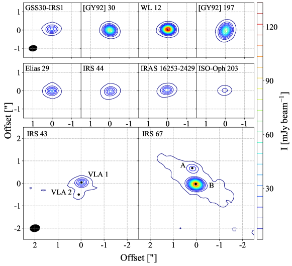
Figure 1: Continuum emission of the detected sources above 5$\sigma$ ($\sigma$ = 0.3 mJy beam^-1). The contours start at 5$\sigma$ and follow a step of 20$\sigma$. The typical synthesised beam is represented by the black filled ellipse in the upper and lower left panels. The (0,0) position represents the position fitted with a 2D Gaussian (see Table 3). The lower panels show the binary systems with the common identifiers of both components.

Table 1: Properties of the observed sources: infrared position, bolometric temperature (T_bol), bolometric luminosity (L_bol), envelope mass (M_env), and other common identifiers.

Source	Infrared position a		Tbol b	Lbol b	Menv c	Other common identifiers
	RA [J2000.0]	Dec [J2000.0]	[K]	[L⊙]	[M⊙]
J162614.6	16 26 14.63	$-$24 25 07.5	7	0.03	0.095	[EDJ2009] 800
GSS30-IRS1	16 26 21.35	$-$24 23 04.3	250	11.00	0.15	Oph-emb 8, [GY92] 6, Elias 21
[GY92] 30	16 26 25.46	$-$24 23 01.3	200	0.12	0.27	Oph-emb 9
WL 12	16 26 44.19	$-$24 34 48.4	380	1.40	0.076	VSSG 30, [GY92] 111
IRAS 16238-2428	16 26 59.10	$-$24 35 03.3	120	1.70	0.045	[EDJ2009] 856
[GY92] 197	16 27 05.24	$-$24 36 29.6	120	0.18	0.16	Oph-emb 6, LFAM 26
Elias 29	16 27 09.40	$-$24 37 18.6	420	18.00	0.045	Oph-emb 16, [GY92] 214
IRS 43 d	16 27 26.91	$-$24 40 50.7	300	3.30	0.13	Oph-emb 14, [GY92] 265, YLW 15
IRS 44	16 27 27.98	$-$24 39 33.4	280	7.10	0.057	Oph-emb 13, [GY92] 269, YLW 16
IRAS 16253-2429	16 28 21.61	$-$24 36 23.4	36	0.24	0.15	Oph-emb 1, MMS 126
ISO-Oph 203	16 31 52.45	$-$24 55 36.2	330	0.15	0.072	Oph-emb 15
IRS 67 d	16 32 00.99	$-$24 56 42.6	180	2.80	0.078	Oph-emb 10, L1689S1 3

The observations covered five different line settings, and the choice of species was made specifically to trace different aspects of the structure of protostars. Lines of C¹⁷O, H¹³CO⁺ and C³⁴S were targeted as tracers of disc kinematics, while SO₂ and CH₃OH are expected to trace the warm chemistry in the inner envelope or disc, and C₂H is commonly associated with outer-envelope regions. Two spectral windows consist of 960 channels each with 122.07 kHz (0.11 km s^-1) spectral resolution centred on C¹⁷O J=3$-$2 and C³⁴S J=7$-$6, while the other three contain 1920 channels each with 244.14 kHz (0.22 km s^-1) spectral resolution centred on H¹³CO⁺ J=4$-$3, the CH₃OH J_k=7_k$-$6_k branch at 338.4 GHz, and the CH₃CN 14$-$13 branch at 349.1 GHz. The latter two settings also pick up SO₂ and C₂H transitions. The observed molecular transitions and their parameters are summarised in Table 2.

Table 2: Spectral setup and parameters of the detected molecular transitions.

Molecular transition	Frequency a	Aij a	Eu a	ncrit b
	[GHz]	[s-1]	[K]	[cm-3]
C17O J=3$-$2	337.06110	2.3 $\times$ 10-6	32	3.5 $\times$ 104
C34S J=7$-$6	337.39646	8.4 $\times$ 10-4	50	1.3 $\times$ 107
SO2 J${}_{\mathrm{K_{A}K_{C}}}$=184,14$-$183,15	338.30599	3.3 $\times$ 10-4	197	5.9 $\times$ 107
CH3OH JK=7-1$-$6-1 E	338.34463	1.7 $\times$ 10-4	70	2.0 $\times$ 106
CH3OH JK=70$-$60 A+	338.40868	1.7 $\times$ 10-4	65	2.8 $\times$ 107
H13CO+ J=4$-$3	346.99835	3.3 $\times$ 10-3	42	8.5 $\times$ 106
C2H N=4$-$3, J=9/2$-$7/2, F=5$-$4	349.33774	1.3 $\times$ 10-4	42	2.2 $\times$ 107
C2H N=4$-$3, J=9/2$-$7/2, F=4$-$3	349.39934	1.3 $\times$ 10-4	42	2.3 $\times$ 107

Table 3: Results of 2D Gaussian fits towards the continuum peak of our Oph sources.

Source	RA	Dec	Size a	PA	F0.87mm	S0.87mm (0$\aas@@fstack{\prime\prime}$4) b
	[J2000.0]	[J2000.0]	[$\arcsec$]	[$\degr$]	[mJy]	[mJy beam-1]
GSS30-IRS1	16 26 21.358	-24 23 04.85	0.19 $\pm$ 0.02 $\times$ 0.12 $\pm$ 0.01	96 $\pm$ 9	35.3 $\pm$ 0.7	30.0 $\pm$ 0.3
[GY92] 30	16 26 25.475	-24 23 01.81	0.25 $\pm$ 0.01 $\times$ 0.12 $\pm$ 0.01	28 $\pm$ 1	105.0 $\pm$ 0.5	80.2 $\pm$ 0.2
WL 12	16 26 44.203	-24 34 48.86	0.14 $\pm$ 0.01 $\times$ 0.11 $\pm$ 0.01	60 $\pm$ 11	160.4 $\pm$ 1.0	142.4 $\pm$ 0.5
LFAM 23 c	16 26 59.166	-24 34 59.07	0.09 $\pm$ 0.02 $\times$ 0.05 $\pm$ 0.04	38 $\pm$ 45	17.6 $\pm$ 0.3	16.9 $\pm$ 0.2
[GY92] 197	16 27 05.252	-24 36 30.14	0.44 $\pm$ 0.01 $\times$ 0.13 $\pm$ 0.01	169 $\pm$ 1	128.3 $\pm$ 0.6	71.1 $\pm$ 0.2
Elias 29	16 27 09.416	-24 37 19.20	0.17 $\pm$ 0.02 $\times$ 0.16 $\pm$ 0.02	61 $\pm$ 90	41.2 $\pm$ 0.6	34.1 $\pm$ 0.3
IRS 43 VLA 1	16 27 26.908	-24 40 50.67	0.21 $\pm$ 0.03 $\times$ 0.13 $\pm$ 0.02	96 $\pm$ 17	41.6 $\pm$ 1.9	32.1 $\pm$ 0.9
IRS 43 VLA 2	16 27 26.917	-24 40 51.18	0.36 $\pm$ 0.09 $\times$ 0.2 $\pm$ 0.1	150 $\pm$ 37	7.5 $\pm$ 1.0	3.7 $\pm$ 0.4
IRS 44	16 27 27.988	-24 39 33.93	0.24 $\pm$ 0.03 $\times$ 0.18 $\pm$ 0.03	124 $\pm$ 19	38.6 $\pm$ 1.2	29.1 $\pm$ 0.6
IRAS 16253-2429	16 28 21.620	-24 36 24.17	0.23 $\pm$ 0.02 $\times$ 0.13 $\pm$ 0.02	111 $\pm$ 6	39.8 $\pm$ 0.7	31.9 $\pm$ 0.4
ISO-Oph 203	16 31 52.445	-24 55 36.48	0.14 $\pm$ 0.03 $\times$ 0.05 $\pm$ 0.03	107 $\pm$ 18	11.3 $\pm$ 0.3	10.6 $\pm$ 0.2
IRS 67 A	16 32 00.989	-24 56 42.78	0.5 $\pm$ 0.1 $\times$ 0.3 $\pm$ 0.2	46 $\pm$ 17	35.7 $\pm$ 7.0	16.2 $\pm$ 2.3
IRS 67 B	16 32 00.978	-24 56 43.44	0.22 $\pm$ 0.02 $\times$ 0.14 $\pm$ 0.01	88 $\pm$ 9	155.5 $\pm$ 4.0	125.1 $\pm$ 2.0

The calibration and imaging were done in CASA (McMullin et al. 2007): the complex gains were calibrated through observations of the quasars J1517-2422 and J1625-2527, passband calibration was based on J1924-2914, and flux calibration was based on Titan. A robust weighting with the Briggs parameter set to 0.5 was applied to the visibilities, and the resulting dataset has a typical beam size of 0$\aas@@fstack{\prime\prime}$43 $\times$ 0$\aas@@fstack{\prime\prime}$32 ($\sim$60 $\times$ 40 au), a continuum rms level of 0.3 mJy beam^-1 , and a spectral rms level of 13 and 9 mJy beam^-1 per 0.11 and 0.22 km s^-1, respectively.

3 Results

3.1 Continuum

The sources that show continuum emission at 0.87 mm are listed in Table 3, with the sub-millimetre coordinates, deconvolved sizes, and fluxes calculated by fitting two-dimensional (2D) Gaussians in the image plane. Two of the sources, IRS 43 (Girart et al. 2000) and IRS 67 (McClure et al. 2010), are known binary systems, and their components are separated by $\sim$70 au (0$\aas@@fstack{\prime\prime}$53) and $\sim$90 au (0$\aas@@fstack{\prime\prime}$68) for IRS 43 and IRS 67, respectively. The sources associated with a single continuum peak have diameters from $\sim$20 au (0$\aas@@fstack{\prime\prime}$14 for ISO-Oph 203) to $\sim$60 au (0$\aas@@fstack{\prime\prime}$44 for [GY92] 197) and fluxes from 11.3 mJy (ISO-Oph 203) to 160.4 mJy (WL 12). The deconvolved sizes show that most of the sources are marginally resolved, with the exception of LFAM 23, IRS 43 VLA 2, and IRS 67 A, which are unresolved.

J162614.6 and IRAS 16238-2428 show neither continuum nor molecular line emission; the upper limit is 0.9 mJy beam^-1 (3$\sigma$) for the continuum emission. J162614.6 shows faint emission at 24 $\mu$m and a low concentrated SCUBA core (Jørgensen et al. 2008), suggesting that this source is more likely related with a prestellar core than with a protostar. For IRAS 16238-2428, the separation between its Spitzer position and SCUBA core is 38$\aas@@fstack{\prime\prime}$6 (Jørgensen et al. 2008); the SCUBA core lies beyond the ALMA primary beam ($\sim$18$\arcsec$). However, the continuum emission detected in the same field of view as IRAS 16238-2428 may correspond to a T Tauri source (LFAM 23) that is located $\sim$4$\arcsec$ offset from the Spitzer position that is associated with IRAS 16238-2428. Table 3 presents results from a 2D Gaussian fit for LFAM 23, revealing that it is a point source. However, this source does not show molecular line emission and is therefore not included in the discussion in this paper.

Figure 1 shows the continuum emission of the remaining ten sources. For the binary systems, the continuum also traces the circumbinary material, which is remarkably extended for IRS 67 ($\sim$550 au; for a detailed analysis of IRS 67, see Artur de la Villarmois et al. 2018). It is worth mentioning that IRS 43 VLA 1 and IRS 67 B are brighter than IRS 43 VLA 2 and IRS 67 A at 0.87 mm, while the opposite situation is observed at infrared wavelengths (Haisch et al. 2002; McClure et al. 2010).

3.2 Molecular lines

The molecular transitions trace different components and are related with different morphologies. Some of them are detected towards the source position, while others peak offset from the source, and the emission may present compact or extended structures. Table 4 summarises the regions where the individual molecular transitions are detected, specifying if the emission is compact or extended (with respect to the extent of the continuum emission), and the source velocity (V_source). The latter is estimated by visual inspection of C¹⁷O emission, or SO₂ emission when C¹⁷O is not detected. For sources where no molecular line emission is detected, V_source is taken from the literature (see Table 4). The two C₂H lines listed in Table 2 are both hyperfine transitions, and the C₂H emission arises from a blended doublet, C₂H N=4$-$3, J=9/2$-$7/2, F=5$-$4 plus C₂H N=4$-$3, J=9/2$-$7/2, F=4$-$3. Emission of at least one molecular transition is detected towards eight of the ten sources. WL 12 (the brightest continuum source) and ISO-Oph 203 (the weakest continuum source) are the only sources where no line emission is detected within the spectral setting shown in Table 2.

3.2.1 Optically thin tracers: C¹⁷O, H¹³CO⁺ , and C³⁴S

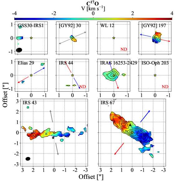
Figure 2: Moment 0 (black contours) and moment 1 (colour scale) maps for C¹⁷O J=3-2 above 5$\sigma$ and integrated over a velocity range of 8 km s^-1. The contours start at 5$\sigma$ and follow a step of 4$\sigma$ ($\sigma$ = 4 mJy beam^-1 km s^-1). The yellow star indicates the position from a 2D Gaussian fit, and the black stars in the lower panels represent the position of the binary components. The arrows show the outflow direction from the literature, where the blue and red represent blue- and red-shifted emission, respectively, and the grey arrow represents infrared observations. The typical synthesised beam is shown by the black filled ellipse in the upper and lower left panels. The ND label marks a non-detection.

Figure 3: Same as Fig. 2 for H¹³CO⁺ J=4$-$3, integrated over a velocity range of 10 km s^-1. The contours start at 5$\sigma$ and follow a step of 3$\sigma,$ with the exception of IRS 67, which follows a step of 6$\sigma$.

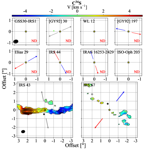
Figure 4: Same as Fig. 2 for C³⁴S J=7$-$6, integrated over a velocity range of 10 km s^-1. The contours start at 5$\sigma$ and follow a step of 3$\sigma,$ with the exception of IRS 43, which follows a step of 6$\sigma$.

C¹⁷O, H¹³CO⁺ , and C³⁴S are less abundant isotopologues, and they are expected to be optically thin tracers associated with the disc kinematics. For example, a Keplerian disc was detected towards the Class 0/I source R CrA in similar C¹⁷O observations with ALMA (Lindberg et al. 2014).

Figure 2 shows moment 0 and 1 maps for C¹⁷O, indicating the outflow direction, if available, from the literature (Bontemps et al. 1996; Allen et al. 2002; van der Marel et al. 2013; Zhang et al. 2013; White et al. 2015; Yen et al. 2017). Five of the sources, [GY92] 30, [GY92] 197, IRAS 16253-2429, IRS 43, and IRS 67, show on-source C¹⁷O emission, and with the exception of IRAS 16253-2429, they are associated with a rotational profile perpendicular to the outflow direction, consistent with a disc-like structure (Sect. 4.2). In addition, the binary systems (IRS 43 and IRS 67) show C¹⁷O emission that is much more extended than towards the other sources: 6$\aas@@fstack{\prime\prime}$1 diameter for IRS 43, 5$\aas@@fstack{\prime\prime}$4 for IRS 67, 1$\aas@@fstack{\prime\prime}$3 for IRAS 16253-2429, 0$\aas@@fstack{\prime\prime}$9 for [GY92] 197, and 0$\aas@@fstack{\prime\prime}$7 for [GY92] 30. The emission towards IRAS 16253-2429 is slightly elongated in the direction perpendicular to the outflow axis and is associated with low velocities (¡ $\pm$2 km s^-1). This low-velocity component may be tracing infalling material from the inner envelope (see detailed discussion in Sect. 4.2).

Figures 3 and 4 show images of the H¹³CO⁺ and C³⁴S emission. H¹³CO⁺ is detected towards only three of the ten sources: IRS 44 and the two binary systems, IRS 43 and IRS 67. IRS 44 shows a velocity gradient with two components, one consistent with the outflow direction, and the another rotated by $\sim$45$\degr$. The peak of emission (moment 0), however, is related with more quiescent material. The more massive of the binary systems (IRS 67) shows more extended emission, and its velocity profile is perpendicular to the outflow direction, while the emission towards IRS 43 is concentrated in the inner regions ($\leq$ 1$\arcsec$) and a tentative velocity gradient is detected. In addition, C³⁴S is solely seen towards the binary systems. IRS 43 shows a velocity gradient perpendicular to the infrared jet direction and the emission peaks spatially offset from the system ($\sim$2$\arcsec$), where the red-shifted emission stands out. A different situation is observed for IRS 67: it has no clear velocity gradient and shows isolated peaks of emission that are spatially offset from the system.

Table 4: Regions where the individual molecular transitions are detected above 3$\sigma$ towards each source and the estimated source velocity (V_source).

Source	Molecular transitions						Vsource a
	C17O	H13CO+	C34S	SO2	CH3OH	C2H	[km s-1]
GSS30-IRS1	Offset	-	-	On source [C]	-	-	3.4
[GY92] 30	On source [C]	-	-	-	Offset	Offset	3.1
WL 12	-	-	-	-	-	-	4.0 b
[GY92] 197	On source	-	-	-	-	On source [C]	3.1
Elias 29	Offset	-	-	On source [C]	-	-	3.6
IRS 43	On source [E]	On source	On source [E]	On source B [C]	-	Offset	4.0
IRS 44	-	On source [E]	-	On source [C]	-	-	2.3
IRAS 16253-2429	On source [E]	-	-	-	-	On source [E]	4.0
ISO-Oph 203	-	-	-	-	-	-	4.5 b
IRS 67	On source [E]	On source [E]	Offset	On source B [C]	-	On source [E]	4.2

3.2.2 Warm chemistry tracers: CH₃OH and SO₂

Figure 5: Observed CH₃OH spectra (blue) towards the 10 sources that show continuum emission, superimposed on the predicted CH₃OH spectrum (red) for a column density of 2.5 $\times$ 10¹⁵ cm^-2, $\sim$4 orders of magnitude below the value from the Class 0 source IRAS 16293-2422 (Jørgensen et al. 2016).

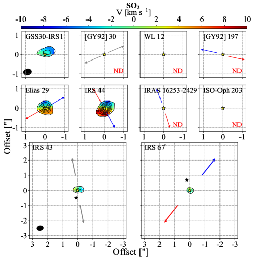
Figure 6: Same as Fig. 2 for SO₂ J${}_{\mathrm{K_{A}K_{C}}}$=18_4,14$-$18_3,15, integrated over a velocity range of 20 km s^-1. The contours start at 5$\sigma$ and follow a step of 20$\sigma$.

Figure 7: Same as Fig. 2 for the doublet C₂H N=4$-$3, J=9/2$-$7/2.

CH₃OH forms exclusively on ice-covered dust grain surfaces because gas-phase reactions produce negligible CH₃OH abundances (Garrod et al. 2006; Chuang et al. 2016; Walsh et al. 2016). When the temperature reaches $\sim$90 K, CH₃OH thermally desorbes from the grain mantles, and its gas-phase abundance is enhanced close to the protostar (Brown & Bolina 2007). Therefore, CH₃OH transitions associated with high rotational levels, such as J=7_k$-$6_k, are expected to trace the warm gas close to the protostar.

The observed CH₃OH J=7_k$-$6_k branch includes transitions with E_u from 65 to 376 K, but no significant emission is detected towards the continuum position from a 2D Gaussian fit of any source (see Table 3). This is highlighted in Fig. 5, where the observed and predicted spectrum are plotted together. The predicted spectrum is obtained using the statistical equilibrium radiative transfer code (RADEX; van der Tak et al. 2007) and assuming local thermodynamic equilibrium (LTE), a CH₃OH column density of 2.5 $\times$ 10¹⁵ cm^-2 ($\sim$4 orders of magnitude below the CH₃OH column density measured towards the Class 0 source IRAS 16293-2422; Jørgensen et al. 2016), and a kinetic temperature (T_kin) of 100 K. Clearly, no CH₃OH lines are seen even at this level.

Nevertheless, [GY92] 30 is a peculiar case (the least luminous source of the sample, L_bol = 0.12 L_⊙, and the source associated with the more massive envelope, M_env = 0.27 M_⊙), where two CH₃OH transitions are detected offset from the source, beyond the 25$\sigma$ continuum contour (Figs. 14 and 15 in the Appendix). These transitions are associated with the lowest E_u levels (65 and 70 K) and the emission is related with low velocities of between $-$0.5 and 0.5 km s^-1 from the source velocity. Thus, the CH₃OH emission towards [GY92] 30 is likely related with extended envelope material. In addition, there is no clear association between the CH₃OH emission and the direction of the infrared jet.

SO₂ is commonly associated with outflows and shocked regions (e.g. Jørgensen et al. 2004; Persson et al. 2012; Podio et al. 2015; Tabone et al. 2017). In addition, the highly excited rotational transitions (E_u $\sim$200 K) may be tracing warm shocked gas. The observed SO₂ transition, listed in Table 2, is associated with a high rotational level (E_u = 197 K) and is detected towards five of the sources, showing compact emission (Fig. 6). A rotational profile is seen for Elias 29 and IRS 44, associated with high velocities (up to $\pm$10 km s^-1 with respect to the source velocity), and almost perpendicular to the outflow direction. Towards the binary systems, the SO₂ emission is relatively weak and detected around one of the sources, IRS 43 VLA1 and IRS 67 B; the sources correspond to the brightest components at 0.87 mm. In addition, GSS30-IRS1 shows only a blue-shifted component, without a clear velocity profile. The SO₂ emission towards Elias 29 and IRS 44 may be consistent with a disc-like structure, but the broad-line profile suggests that SO₂ traces a different component that is associated with warm shocked gas.

3.2.3 Outer envelope tracer: C₂H

The emission of C₂H has been associated with dense regions exposed to UV radiation (e.g. Nagy et al. 2015; Murillo et al. 2018). Its emission is shown in Fig. 7 and is detected towards five of the sources. Two of the them, [GY92] 197 and IRAS 16253-2429, show on-source emission related with low velocities, showing a compact morphology for [GY92] 197 and an extended structure for IRAS 16253-2429. Towards [GY92] 30, IRS 43, and IRS 67, there is no C₂H emission (above 5$\sigma$) at the positions of the sources, but a velocity gradient is seen for the circumbinary material, with a remarkable extended emission for IRS 67 ($\sim$9$\arcsec$). Because IRAS 16253-2429 has one of the most massive envelopes (M_env = 0.15 M_⊙) and circumbinary discs are usually related with a higher mass content and greater extension than circumstellar discs, C₂H likely traces more dense regions.

4 Mass evolution

The final mass of a protostar and the amount of material available in the disc to form planets depend on the mass evolution of the whole system (envelope, disc, protostar, and outflow). Determining when and how quickly the envelope dissipates and the disc grows in mass and size, the rate at which the protostar gains mass and the amount of material expelled through the outflows are all linked to each other and are crucial components in the mass evolution. In this section, we estimate the disc masses from the continuum emission (Sect. 4.1) and the stellar masses from molecular lines that show Keplerian profiles (Sect. 4.2). Later on, a comparison between envelope mass, disc mass, stellar mass, and bolometric luminosity is presented (Sect. 4.3). Finally, the mass accretion rate is estimated from a relationship between the stellar mass and the bolometric luminosity, and this is compared with the bolometric temperature.

4.1 disc mass

The disc masses (M_disc) were calculated from the continuum fluxes (F_0.87mm), listed in Table 3, and

$$M_{\mathrm{disc}}=\frac{S_{\nu}d^{2}}{\kappa_{\nu}B_{\nu}(T)}\ ,$$ (1)

where S_ν is the surface brightness, d is the distance to the source, $\kappa$_ν is the dust opacity, and B_ν(T) is the Planck function for a single temperature. A distance of 139 $\pm$ 6 pc (Mamajek 2008) and $\kappa$_0.87mm of 0.0175 cm² g^-1 (Ossenkopf & Henning 1994), commonly used for dust in protostellar envelopes and young discs in the millimetre regime (e.g. Shirley et al. 2011), was adopted for the calculations (Artur de la Villarmois et al. 2018). A value of 15 K was adopted for the dust temperature (T_dust) following the analysis by Dunham et al. (2014b). The calculated disc masses (gas + dust, assuming a gas-to-dust ratio of 100) are listed in Table 5, together with values from the literature. Errors in T_dust are not considered in Table 5, but the disc masses will decrease by a factor of $\sim$3 when a dust temperature of 30 K is assumed instead (found to be appropriate for Class 0 sources in the study by Dunham et al. 2014b). For WL 12, Elias 29, and IRS 43, disc masses are available from other studies (see Table 5). For Elias 29 and IRS 43, the values from this work are comparable with the literature, and the difference seen for WL 12 appears to be due to the choice of dust temperature (15 vs. 30 K). Assuming T_dust = 30 K, a value of (10.3 $\pm$ 2.4) $\times$ 10^-3 M_⊙ is found for M_disc associated with WL 12.

Table 5: Calculated disc masses for T_dust = 15 K and values from the literature.

Source	Mdisc [10-3 M⊙]
	This work	Literature
GSS30-IRS1	6.2 $\pm$ 0.6
[GY92] 30	18.5 $\pm$ 1.6
WL 12	28.3 $\pm$ 2.4	11 a
LFAM 23	3.1 $\pm$ 0.3
[GY92] 197	22.6 $\pm$ 2.0
Elias 29	7.3 $\pm$ 0.6	11 a
		¡ 7 b
IRS 43 VLA 1	7.3 $\pm$ 0.7	8 a
IRS 43 VLA 2	1.3 $\pm$ 0.2
IRS 44	6.8 $\pm$ 0.6
IRAS 16253-2429	7.0 $\pm$ 0.6
ISO-Oph 203	2.0 $\pm$ 0.2
IRS 67 A	6.3 $\pm$ 1.3
IRS 67 B	27.4 $\pm$ 2.5

4.2 Stellar mass

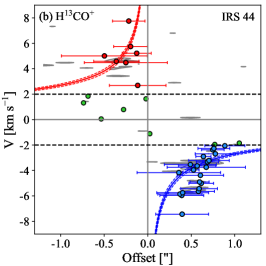
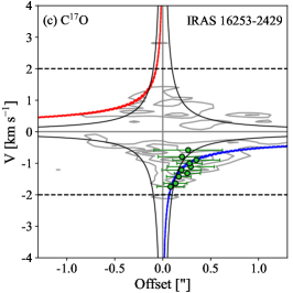
Figure 8: Position-velocity diagrams towards [GY92] 197, IRS 44 and IRAS 16253-2429. Blue and red dots represent blue- and red-shifted emission peaks above $\pm$2 km s^-1, respectively, while green dots indicate velocities below $\pm$2 km s^-1. Blue and red solid lines show the best fit for a Keplerian velocity profile with their respective errors, shown in dashed blue and red lines. The cut taken from the image data is shown in grey contours, ranging from 3$\sigma$ ($\sigma$ = 13 mJy beam^-1) to the maximum value of each transition. Each adjacent contour represents an increment of 30$\%$ of the maximum value for panels (a) and (c), and an increment of 50$\%$ for panel (b). The black dashed lines indicate the velocity above which the Keplerian profile was fitted. The solid black curves in panel (c) show the best fit for an infalling velocity profile.

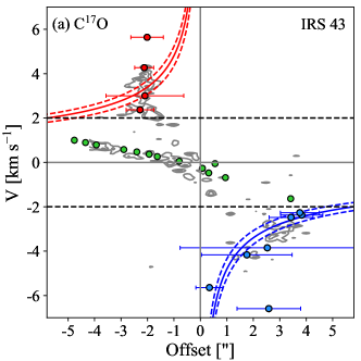
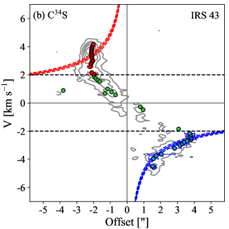
Figure 9: Position-velocity diagrams for C¹⁷O and C³⁴S towards IRS 43. Blue and red dots represent blue- and red-shifted emission peaks above $\pm$2 km s^-1, respectively, while green dots indicate velocities below $\pm$2 km s^-1. Blue and red solid lines show the best fit for a Keplerian velocity profile with their respective errors, shown in dashed blue and red lines. The cut taken from the image data is shown in grey contours, ranging from 3$\sigma$ ($\sigma$ = 13 mJy beam^-1) to the maximum value of each transition. Each adjacent contour represents an increment of 30 and 20$\%$ of the maximum value for C¹⁷O and C³⁴S, respectively. The black dashed lines indicate the velocity above which the Keplerian profile was fitted.

In order to investigate whether the optically thin tracers are associated with Keplerian motions and to estimate the stellar masses (M_⋆), position-velocity (PV) diagrams were created for the sources that show disc-like structures in C¹⁷O, H¹³CO⁺ or C³⁴S. The peak emission for each channel was obtained through the CASA task imfit, and the offset position was calculated by projecting the peak emission onto the disc position angle (Table 3). Next, a Keplerian profile ($v$ $\propto$ r^-0.5) was employed to fit the points with velocities above $\pm$2 km s^-1. This velocity range was chosen in order to avoid the envelope contribution (e.g. van ’t Hoff et al. 2018). The PV diagrams and peak points are shown in Figs. 8 and 9, and the resulting Keplerian curve from the fit is overplotted. Figure 8a shows a robust Keplerian profile for [GY92] 197, while the PV diagram for IRS 44 is noisy (Fig. 8b), with an unclear Keplerian profile. IRAS 16253-2429 shows low-velocity emission ($\leq$2 km s^-1) and both negative and positive velocities for the same distance to the source (see Fig. 8c). This is a characteristic feature of infalling material (e.g. Tobin et al. 2012). Therefore, these points were fitted with an infalling profile under the conservation of angular momentum ($v$ $\propto$ r^-1; e.g. Lin et al. 1994; Harsono et al. 2014). The resulting stellar masses are listed in Table 6, adopting an inclination (i) of 70$\degr$ from the plane of the sky. This value is adopted from the mean value of the inclination of the sample, calculated from the deconvolved continuum sizes (Table 3) and assuming a circular structure. In addition, 70$\degr$ is consistent with values from the literature: 70$\degr$ for IRS 43 (Brinch et al. 2016) and 60$\degr$ for IRAS 16253-2429 (Yen et al. 2017). The stellar mass changes by less than 14$\%$ when the inclination varies with $\pm$10$\degr$.

IRS 43 shows extended emission in C¹⁷O and C³⁴S, with PV diagrams and Keplerian fits shown in Fig. 9 for both molecular transitions. The blue-shifted C³⁴S emission is well fitted with a Keplerian profile, but the red-shifted emission shows an enhancement around 2$\arcsec$ and a vertical velocity structure, from $\sim$2 to $\sim$4 km s^-1. PV diagrams for IRS 67 from C¹⁷O and H¹³CO⁺ emission are presented in Artur de la Villarmois et al. (2018).

Table 6 lists the stellar masses obtained from PV diagrams and values from the literature. For IRS 43, the stellar masses inferred from a Keplerian fit from C¹⁷O and C³⁴S emission are a factor of 2 higher than the 1.80 M_⊙ from Brinch et al. (2016). To be consistent within the sample, the stellar mass of 4.0 M_⊙ is used for the IRS 43 system hereafter. For IRAS 16253-2429, the stellar mass from Yen et al. (2017) is consistent with our value from the fit for the infalling gas.

Table 6: Stellar masses obtained from the velocity profile fits and values from the literature.

Source		This work		Literature
		M⋆ [M⊙] a	Molecule			M⋆ [M⊙]	Method
[GY92] 197		0.23 $\pm$ 0.02	C17O
Elias 29						2.5 $\pm$ 0.6 b	HCO+ J=3$-$2 emission
IRS 43		4.0 $\pm$ 0.3	C34S			1.80 $\pm$ 0.42 c	HCN J=3$-$2 emission
		3.9 $\pm$ 0.7	C17O
IRS 44		1.2 $\pm$ 0.1	H13CO+
IRAS 16253-2429		0.03 $\pm$ 0.02	C17O (infalling)			0.03 $\pm$ 0.01 d	C18O J=2$-$1 emission
IRS 67 e		2.2 $\pm$ 0.2	C17O

4.3 Mass evolution

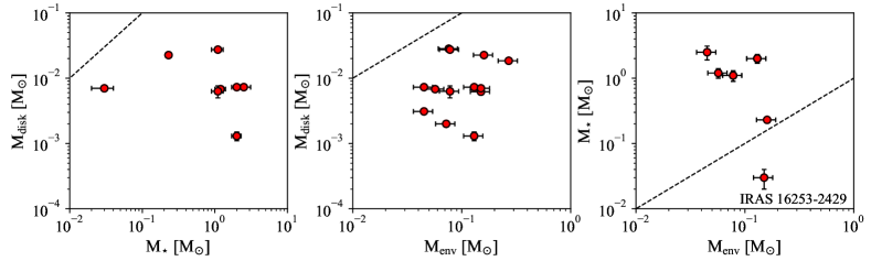
Figure 10: Comparison between disc mass and stellar mass (left), disc mass and envelope mass (centre), and stellar mass and envelope mass (right). The dashed black line is for M_i = M_j.

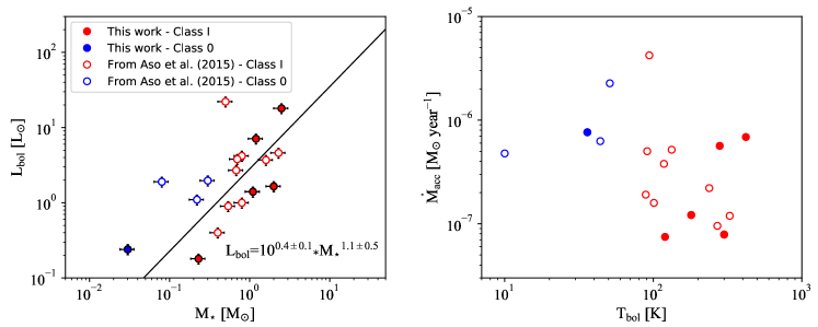
Figure 11: Left: Bolometric luminosity as a function of stellar mass with data points from this work and from Aso et al. (2015). The black straight line shows the best fit for all Class I sources. Right: Mass accretion rate as a function of the bolometric temperature.

Figure 10 compares the envelope masses (M_env; Table 1), disc masses (M_disc; Table 5), and stellar masses (M_⋆; Table 6). The uncertainties in M_env are assumed to be 20$\%$. There is no clear trend between M_disc and M_⋆ or M_env, however, all the points satisfy the condition M_⋆ ¿ M_disc and M_env ¿ M_disc, characteristic of Class I stages (Robitaille et al. 2006). For M_⋆ as a function of M_env, the stellar mass increases as the mass of the envelope decreases, and only one of the sources (IRAS 16253-2429) satisfies the condition M_env ¿ M_⋆, which is a characteristic of Class 0 protostars. This is also consistent with its low bolometric temperature, T_bol of 36 K, and the infalling profile for the gas kinematics.

The left panel of Fig. 11 shows the bolometric luminosities as a function of stellar masses from Table 6 and values of Class 0 and I sources summarised in Aso et al. (2015) (see Table 8 in the Appendix). The uncertainties in M_⋆ and L_bol are 20$\%$ and 15$\%$, respectively (e.g. Yen et al. 2017), and for the particular case of the binary systems (IRS 43 and IRS 67), the M_⋆ and L_bol values were divided by 2 to account for each component. For Class I sources, the correlation between L_bol and M_⋆ appears to be linear, with one outlier that corresponds to the source L1551 IRS 5. The straight line in Fig. 11 shows the best fit for all Class I sources, providing the following power-law relationship:

$$L_{\mathrm{bol}}=10^{0.4\pm 0.1}M_{\star}^{1.1\pm 0.5}.$$ (2)

Assuming that L_bol results from the gravitational energy that is released by the material accreted onto the surface of the protostar, the mass accretion rate ($\dot{M}$_acc) can be estimated from

$$\dot{M}_{\mathrm{acc}}=\frac{L_{\mathrm{bol}}R_{\star}}{GM_{\star}}\ ,$$ (3)

where R_⋆ is the protostellar radius and G the gravitational constant. Assuming R_⋆ = 3R_⊙ (Stahler et al. 1980), the calculated accretion rates are shown in the right panel of Fig. 11 as a function of T_bol. Combining Eqs. 2 and 3, a value of (2.4 $\pm$ 0.6) $\times$ 10^-7 M_⊙ year^-1 is obtained for $\dot{M}$_acc for the Class I sources, with a minimum and maximum value of 7.5 $\times$ 10^-8 and 7.6 $\times$ 10^-7 M_⊙ year^-1, respectively. The mean value is consistent with the mass accretion rates from Yen et al. (2017), who found $\dot{M}$_acc from $\sim$1 $\times$ 10^-7 to 4.4 $\times$ 10^-6 M_⊙ yr^-1 for a sample of Class I sources. The right panel of Fig. 11 shows $\dot{M}$_acc as a function of T_bol. Myers & Ladd (1993) defined T_bol as the temperature of a blackbody that has the same mean frequency as the observed continuum spectrum, and this is often taken as an indicator of the evolutionary stage of the source (e.g. Dunham et al. 2014a; Frimann et al. 2016a; Fischer et al. 2017). A tentative decrease in $\dot{M}$_acc as the systems evolve is seen in Fig. 11. Nevertheless, the trend is not clear, and the sample of Class 0 sources is still small.

When the accretion rate is assumed to be constant (2.4 $\times$ 10^-7 M_⊙ year^-1), a typical Class I protostar will reach 1 M_⊙ in $\sim$4 Myr, which is inconsistent with the derived lifetime for the embedded Class 0/I phase (from 0.13 to 0.78 Myr; Dunham et al. 2015; Kristensen & Dunham 2018). This inconsistency is know as the luminosity problem (Kenyon & Hartmann 1995), where a constant accretion rate cannot explain the low luminosities of embedded protostars. With interferometric facilities, the stellar masses are better constrained from molecular line emission, and the only way to reconcile theory with observations is to assume a time-variable accretion rate onto the protostar (Kenyon & Hartmann 1995; White et al. 2007; Evans et al. 2009; Vorobyov & Basu 2010; Dunham & Vorobyov 2012; Audard et al. 2014; Dunham et al. 2014a). The time-variable or burst model of accretion operates in the embedded phase of protostellar evolution, and the disc spends practically all of its time in a low state (low $\dot{M}$_acc) and accretes significant mass in relatively short bursts, which would account for the low average L_bol of protostars (Vorobyov & Basu 2010; Dunham et al. 2014a).

In Fig. 11, L1551 IRS 5 is the only Class I source with high L_bol and high $\dot{M}$_acc that stands out over the others. This source has been proposed to be a young star experiencing an FU Ori-like outburst (Hartmann & Kenyon 1996; Osorio et al. 2003). With the exception of L1551 IRS 5, the rest of the Class I sources in this sample appear to be in a low state of accretion (see Table 8 in the Appendix).

If the accretion onto the central star is episodic, the accretion bursts may have strong effects on the chemistry. In consequence, observable chemical effects (such as the C¹⁸O spatial distribution) can provide clues to the luminosity history (e.g. Jørgensen et al. 2013, 2015; Frimann et al. 2016b). In our sample, the lack of significantly extended C¹⁷O emission contrasts with the C¹⁸O emission observed by Jørgensen et al. (2015) and Frimann et al. (2016b) towards a different sample of Class 0/I sources, which suggests a relatively quiescent phase for our sources or a low C¹⁷O column density at larger distances from the source.

5 Chemical evolution

5.1 Line emission as a function of L_bol and T_bol

The differences in the molecular emission signatures for the sources in the sample may be an indication that the chemistry does depend on the physical evolution of the sources, that is to say, the molecular column densities vary as a function of the source bolometric luminosities and temperatures. For the molecular transitions detected towards the source position, the spectrum was extracted from the pixel that corresponds to the peak of the continuum emission (see Table 3), and a Gaussian fit was applied to the line profile (see Fig. 16 in the Appendix). The resulting values are listed in Table 7 and are estimates of the line intensities towards the peak, and not the full integrated emission over the maps. Most of the line profiles show a single central component centred at V_source. When more than one component is observed, the intensity listed in Table 7 is the sum of all the individual components. For the sources without on-source detection, the 3$\sigma$ upper limit per 1 km s^-1, that is, 0.013 Jy beam^-1 km s^-1, is used in the comparison.

Table 7: Line intensity towards the source position calculated from a Gaussian fit.

Source	Intensity [Jy beam-1 km s-1]
	C17O	C2H	H13CO+	SO2
GSS30-IRS1	-	-	-	0.439
[GY92] 30	0.081	-	-	-
WL 12	-	-	-	-
[GY92] 197	0.226	0.073	-	-
Elias 29	-	-	-	1.036 b
IRS 43 VLA 1	0.049	-	0.133	0.389 b
IRS 43 VLA 2	0.053	-	0.051	-
IRS 44	-	-	0.124	1.478 b
IRAS 16253-2429	0.213	0.206	-	-
ISO-Oph 203	-	-	-	-
IRS 67 A	0.134	-	0.187	-
IRS 67 B	0.488 a	0.077	0.396 a	0.221 b

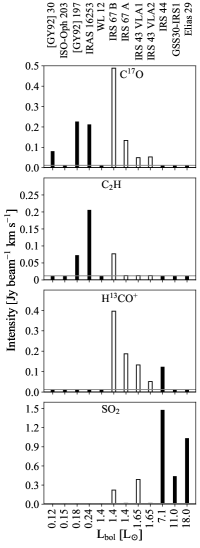
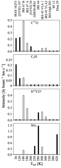
Figure 12: Line intensity as a function of the bolometric luminosity (left) and bolometric temperature (right) towards the source position. The empty bars represent the binary systems, and the grey horizontal line indicates a value of 3$\sigma$.

Figure 12 shows the line intensities from Table 7 as a function of L_bol and T_bol. The binary systems are represented by empty bars in order to distinguish them from the single systems because the former are particularly rich in molecular lines. The binary systems show emission of almost all the transitions presented in Table 2, with the exception of CH₃OH. This chemical richness appears to be related to the mass content and extent of the circumbinary discs, in agreement with the results of Murillo et al. (2018).

Considering only the single sources, C¹⁷O is seen mostly towards the least luminous ones (see upper left panel of Fig. 12), while the opposite situation is the case for SO₂ (lower left panel of Fig. 12). The sources with high bolometric luminosity are associated with high temperatures close to the protostar. This means that for the same continuum flux, the dust mass will be lower for sources with high L_bol, and thus, a lower column density of C¹⁷O is expected. On the other hand, SO₂ traces a different physical process than C¹⁷O and may be related with more energetic processes that are linked to the bolometric luminosity, and thus, the accretion history. If T_bol is taken as an evolutionary indicator, C¹⁷O and C₂H emission are associated with the less evolved sources. In particular, Figs. 2, 7, and 12 show a trend between the extent of the C¹⁷O and C₂H emission and the evolutionary stage of the source. On the other hand, there is no clear correlation between the sources with detected H¹³CO⁺ emission and L_bol or T_bol.

Figure 13 shows the chemical signatures in a plot of L_bol as a function of T_bol for the sources that were observed as part of this study with additional points from the literature: Class 0 sources from Dunham et al. (2015) and Class I sources from Harsono et al. (2014). Three groups of sources can be identified based on on-source detections. The least evolved and luminous sources show C¹⁷O emission towards the source position, while the more evolved and luminous sources are associated with SO₂ emission. In addition, the more evolved sources associated with low luminosities do not show any line detection. As the system evolves from Class 0 to Class I and later to Class II, the envelope mass decreases, leading to a lower gas column density and lines may be harder to detect. This is reflected in the emission of a high-density tracer, such as C¹⁷O: the extent of the emission decreases with the evolutionary stage of the source, followed by a non-detection towards the more evolved sources. For the latter, emission of more abundant isotopologues, such as C¹⁸O and ¹³CO, is expected to be seen, as in Class II sources. On the other hand, there is a chemical differentiation between C¹⁷O and SO₂, where the latter may be tracing a more energetic process that is probably linked to higher accretion rates, which is mostly determined by inner disc properties. Future observations of CO isotopologues and SO₂ transitions with different E_u values towards a larger sample of Class I sources will provide a more statistical perspective.

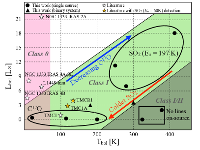
Figure 13: Bolometric luminosity as a function of the bolometric temperature, highlighting the regions where specific molecular transitions are detected towards the source position, and well-known Class 0 and I sources from Dunham et al. (2015) and Harsono et al. (2014), respectively. This plot only covers the lines listed in Table 2 plus SO₂ 11_1,11$-$10_0,10 from Harsono et al. (2014). The Class 0 covers T_bol $\leq$ 70 K (Dunham et al. 2014b), and the Class I/II region includes the sources where no line emission is detected.

5.2 Absence of warm CH₃OH emission

One of the chemical results of this study is the absence of compact CH₃OH emission towards all of the sources. At large scales, CH₃OH is found to be in solid form with typical abundances with respect to water, CH₃OH:H₂O, of about 5$\%$ (Bottinelli et al. 2010; Öberg et al. 2011; Boogert et al. 2015). CH₃OH is expected to sublimate off dust grains in the inner envelopes and in the protostellar discs in regions where the temperature increases above $\sim$90 K (Brown & Bolina 2007). Such warm CH₃OH has been inferred for some Class 0 sources based on single-dish observations (e.g. van Dishoeck et al. 1995; Schöier et al. 2002; Maret et al. 2005; Jørgensen et al. 2005b; Kristensen et al. 2010) and it has also been imaged with interferometers (e.g. Jørgensen et al. 2005a; Maury et al. 2014; Jørgensen et al. 2016; Higuchi et al. 2018).

The absence of CH₃OH line emission provides strict upper limits to the column densities of the warm gas-phase CH₃OH. The upper limit to the column density is estimated using the predictions for a synthetic spectrum for methanol calculated under the assumption of LTE and adopting a kinetic temperature of 100 K and a typical line width of 5 km s^-1. For the 3$\sigma$ rms noise in the spectra of 13 mJy beam^-1 km s^-1, this corresponds to an upper limit for the column density of 5 $\times$ 10¹⁴ cm^-2 (assuming that the emission fills the beam uniformly), which is more than four orders of magnitude below that of the Class 0 protostar IRAS 16293-2422 (Jørgensen et al. 2016). As an illustration, Fig. 5 shows the calculated synthetic spectrum for a column density that is higher than this by a factor of five (i.e. 2.5 $\times$ 10¹⁵ cm^-2).

The low upper limit for the CH₃OH column density implies that (i) there is no hot-core-like region in the inner envelope close to the protostar if its envelope density profile can be extrapolated to the smallest scales and (ii) the gas-phase CH₃OH averaged over the entire disc is low. For the warm gas in the inner envelope, the column density can be translated into a constraint on the abundance by comparing to the results from Lindberg et al. (2014) for the Class 0/I protostar R CrA IRS 7B: through line radiative transfer modelling of ALMA detections of the same CH₃OH lines, Lindberg et al. (2014) found a CH₃OH abundance of 10^-10 in the inner region of the 2.2 M_⊙ envelope. The average envelope mass for our sample is 0.11 M_⊙, which is an order of magnitude below that from R CrA IRS 7B, and because our beam size and distance are similar to those of R CrA IRS 7B and our upper limits comparable to the brightest lines in the spectra from Lindberg et al. (2014), the upper limit to the CH₃OH abundance for our sources should be about an order of magnitude higher than the inferred abundance for R CrA IRS 7B, that is, $\sim$10^-9. Conversely, by ignoring the envelope, an upper limit to the CH₃OH abundance for the disc can be estimated by comparing the inferred disc mass from the ALMA dust continuum measurements to the upper limit of the CH₃OH column density assuming that both fill the beam uniformly. Adopting an average disc mass of 0.0085 M_⊙ for our sample and the upper limit to the CH₃OH column density of 5 $\times$ 10¹⁴ cm^-2, the corresponding upper limit for the CH₃OH abundance is 10^-10, averaged over the entire disc.

These numbers may seem at odds with the results from ice measurements mentioned above, with CH₃OH at least of order 1$\%$ relative to water, which in turn has a typically quoted abundance ([H₂O]/[H₂]) of $10^{-4}$ (Boogert et al. 2015). However, in both cases the assumptions of the physical structures are critical: for example, Lindberg et al. (2014) showed for the protostellar envelope that the CH₃OH abundance would increase by two orders of magnitude if a constant density profile were used at scales smaller than the disc size (corresponding to the flattening of the inner envelope in rotating collapse), rather than a centrally peaked power-law envelope density profile as expected from free-fall. Because a number of sources in our sample show evidence for resolved discs, it is reasonable to apply the same argument, that is, the upper limit to the CH₃OH abundance would be 10^-7 (rather than 10^-9), which is comparable to the estimates for hot cores towards Class 0 protostars (e.g. Schöier et al. 2002; Maret et al. 2005; Jørgensen et al. 2005b). Likewise, for the disc argument, Persson et al. (2016) showed that in simple parametrised disc models, only a small fraction, as low as 1$\%$, of the total disc mass may have temperatures above 100 K where water could sublimate. These are the regions where CH₃OH would also be in the gas phase, thus the upper limit for the CH₃OH abundance in the warm parts of the discs would likewise be less stringent, $\sim$10^-8. Furthermore, by analysing the H₂¹⁸O emission towards 4 Class 0 sources, Persson et al. (2016) showed that the H₂O abundance in the warm regions of the discs could be as low as 10^-7–10^-6, which would be consistent with the CH₃OH abundance limit derived above for typical CH₃OH:H₂O ice abundance ratios of $\sim$1$\%$.

Obviously, there are still a number of caveats in this analysis, in particular, about the physical structure of the material towards protostars at these small scales. Open questions are for instance the density profiles of the envelopes and the temperature structures of the embedded discs. It can therefore not be ruled out that the absence of CH₃OH is still to some degree caused by chemical effects such as the suppression of methanol formation that is due to higher temperatures in the precursor environments, as also discussed for the case of Corona Australis by Lindberg et al. (2014). Future modelling efforts and observation of lower-excited CH₃OH transitions at large and small scales may provide further insights.

5.3 Does SO₂ trace accretion shocks?

The combination of compact (r ¡ 0$\aas@@fstack{\prime\prime}$5 or 70 au; see Fig.6) high-velocity emission (up to $\pm$10 km s^-1; see Fig.16) and the velocity gradient perpendicular to the outflow direction suggests that the warm SO₂ emission may be tracing warm shocked material, in particular, accretion shocks. Material from the inner envelope falls onto the circumstellar disc and produces accretion shocks at the envelope-disc interface, releasing molecules from the dust grains and altering the chemistry. Miura et al. (2017) investigated the thermal desorption of molecules from the dust-grain surface by accretion shocks and found that the enhancement of some species (such as SO) can be explained by the accretion shock scenario, where the main parameters are the grain size, the pre-shock gas number density, and the shock velocity. Taking a shock velocity of 10 km s^-1, Miura et al. (2017) predicted that SO₂ can be released from the dust-grain surface for a pre-shock gas number density of $\sim$10⁷ cm^-3.

Another formation path for SO₂ is by oxidation of SO in the gas phase (Charnley 1997):

$$\mathrm{SO+OH\rightarrow SO_{2}+H},$$ (4)

which is very efficient for T between 100 and 200 K. In this scenario, the SO₂ abundance depends strongly on the presence of SO and OH in the gas phase. SO can be released from dust grains at lower velocities and densities than SO₂, since SO has a lower desorption energy (E_d0) than SO₂ (2600 K and 3400 K for SO and SO₂, respectively; Wakelam et al. 2015; Miura et al. 2017). In addition, OH is seen towards Class I sources and has been associated with shocked regions in the inner envelope close to the protostar (Wampfler et al. 2013). In order to test these two scenarios, oxidation of SO or desorption from dust grains, transitions from warm SO (E_u $\sim$200 K) need to be observed.

In addition to SO and SO₂, CH₃OH has also been related with shocked regions (e.g. Avery & Chiao 1996; Jørgensen et al. 2007). This raises the question why CH₃OH is not detected if SO₂ (or SO) is released from the grain surface by accretion shocks. There are two possibilities: (i) CH₃OH is not released from the grain surface because it has a higher desorption energy (E_d0 = 5000 K), therefore, a higher pre-shock gas number density is required ($\sim$10⁸ cm^-3; Miura et al. 2017), or (ii) CH₃OH is released, but is later destroyed by the high velocities. Suutarinen et al. (2014) demonstrated that CH₃OH is sputtered from ices in shocks with v $\geq$ 3 km s^-1, survives at moderate velocities, but is later dissociated for v $\geq$ 10 km s^-1.

A Keplerian disc or disc winds are less plausible scenarios to explain the SO₂ emission. For a Keplerian profile, high velocities ($\geq$ 5 km s^-1) would be reached at scales smaller than 0$\aas@@fstack{\prime\prime}$2 (see Fig.8), therefore, the high-velocity SO₂ component seen at $\sim$0$\aas@@fstack{\prime\prime}$5 (see Fig.6) is not consistent with a Keplerian profile. For disc winds towards Class I sources, it has been shown that species such as SO do not survive beyond $\sim$1 au (Panoglou et al. 2012). In contrast, towards Class 0 sources, a disc wind driven by SO survives between 10 and 100 au (Panoglou et al. 2012), in agreement with what was found towards the Class 0 source HH212: Tabone et al. (2017) proposed that SO and SO₂ are tracing a disc wind and the emission is observed between $\sim$50 and $\sim$150 au. In any case, neither option can be completely ruled out, and higher spatial resolution is required in order to create a PV diagram and obtain a velocity profile for SO₂.

6 Summary

We presented high angular resolution (0$\aas@@fstack{\prime\prime}$4, $\sim$60 au) ALMA observations of 12 Class I sources in the Ophiuchus star-forming region. The continuum emission at 0.87 mm was analysed together with C¹⁷O, C³⁴S, H¹³CO⁺, SO₂, C₂H, and CH₃OH, and the main results are provided below.

Of the 12 sources, 2 show no continuum emission nor molecular line emission, whereas another 2 show continuum emission but no line detection. Two sources are proto-binary systems with very rich line emission, and the remaining 6 sources show continuum emission plus some of the molecular transitions. C¹⁷O is seen towards the less evolved sources and the binary systems, tracing high gas column densities. Keplerian profiles are found for three sources, while an infalling profile is seen for one of them. More abundant isotopologues, such as C¹⁸O and ¹³CO, may be better disc tracers for the more evolved sources.

The non-detection of warm CH₃OH implies that there in no hot-core-like region in the inner envelope close to the protostar (which follows a power-law density profile) and that the averaged CH₃OH column density over the entire disc is low. This suggests that (i) the presence of a disc flattens the envelope density profile at small scales and thus leads to a low column density of warm material, (ii) only a small portion (1$\%$) of the disc may have temperatures above 100 K, or (iii) chemical effects may suppress the formation of methanol. Clearly, future modelling efforts and observations of colder CH₃OH at envelope and disc scales are required in order to provide stronger conclusions.

Warm (E_u = 197 K) and compact (r ¡ 70 au) SO₂ emission is detected towards five of the sources, with particularly large line widths (between $-$10 and 10 km s^-1) towards Elias 29 and IRS 44. This emission may be related with accretion shocks. The shocks would also liberate CH₃OH from dust mantles, but it would later be destroyed by the high velocities (¿ 10 km s^-1).

The fact that C¹⁷O is detected towards the less evolved and less luminous sources agrees with a decrease in gas column density, which is a consequence of the evolution of the system, and with the low column density of material due to high temperatures. The envelope mass decreases as the system evolves, therefore the gas column density related to quiescent material decreases and lines are hardly detected. However, no similar trend is observed for SO₂ , and instead, a chemical differentiation between C¹⁷O and SO₂ is seen. SO₂ is detected towards the most evolved sources with high L_bol, and is therefore related with higher accretion rates and a different physical process.

The comparison between disc, envelope, and stellar masses shows a trend between M_⋆ and M_env: the most massive stars are related with less envelope material, as expected. In addition, L_bol shows a linear dependence with M_⋆ for Class I sources, where the best fit gives L_bol = 10^0.4±0.1M_⋆^1.1±0.5. Assuming that L_bol is a consequence of accretion onto the protostar, a mean $\dot{M}$_acc of (2.4 $\pm$ 0.6) $\times$ 10^-7 M_⊙ year^-1 is calculated, with values ranging from 7.5 $\times$ 10^-8 to 7.6 $\times$ 10^-7 M_⊙ year^-1. If $\dot{M}$_acc is constant, the time required to accrete enough mass will be greater that the mean lifetime of the embedded stage, supporting the scenario of episodic accretion bursts and a variable accretion rate. Within this scenario, the Class I sources discussed in this work may be in a quiescent phase, with the exception of L1551 IRS 5.

This work shows the importance of a representative sample for exploring the physical and chemical structure of Class I sources, by comparing not only the continuum emission, but also the emission of specific molecules and the protostellar masses obtained from the velocity profiles. The observation of disc and warm gas tracers is crucial in order to interpret the physical and chemical processes and evolution at disc scales. Future observations will provide more statistical results, and the study of other species will contribute to a better understanding of the chemical evolution of low-mass protostars.

Appendix A CH₃OH emission towards [GY92] 30

Two CH₃OH transitions are detected towards [GY92] 30, where the emission peaks beyond the 25$\sigma$ continuum contour and no emission is seen towards the source position (Fig. 14). These transitions are associated with the lowest E_u (65 and 70 K) and the emission is related with low velocities of between $-$0.5 and 0.5 km s^-1 from the source velocity. In addition, they present different morphologies, and the spectra taken towards different positions show a variation in the intensity of both lines. The integrated spectrum towards a region of $\sim$300$\times$600 au is shown in Fig. 15, where both CH₃OH transitions are detected. This emission may be related with quiescent envelope material because [GY92] 30 has the more massive envelope from the sample (see Table 1).

Figure 14: Left: Contour maps of CH₃OH 7_-1$-$6_-1 E and CH₃OH 7₀$-$6₀ A⁺ towards [GY92] 30. The contours start at 3$\sigma$ and follow a step of 3$\sigma$ ($\sigma$ = 4 mJy beam^-1 km s^-1), representing velocities from -0.5 to 0.5 km s^-1. The dashed black contours show the continuum emission for values of 4 and 25$\sigma$. The yellow star indicates the position of the 2D Gaussian fit, and the synthesised beam is represented by the black filled ellipse. The dotted box represents the region from which the spectrum of Fig. 15 is integrated. Right: Spectra towards different positions marked on the contour maps. The grey dashed horizontal line represents a value of 3$\sigma,$ and all the spectra are rebinned by a factor of 4. The dotted black vertical lines indicate the rest frequency of the two CH₃OH transitions.

Figure 15: Integrated spectrum towards the squared region highlighted in the left panels of Fig. 14.

Appendix B Mass accretion rates

The values of L_bol, T_bol, M_⋆, and $\dot{M}$_acc, plotted in Fig. 11, are listed in Table 8. L_bol, T_bol, and M_⋆ are taken from this work and from the literature (see Tables 1 and 6), while $\dot{M}$_acc is calculated from Eq. 3.

Table 8: Bolometric luminosity, bolometric temperature, and stellar masses of Class 0 and I sources from this work and from the literature, with the calculated mass accretion rates.

Source	Lbol	Tbol	M⋆	$\dot{M}$acc	References
	[L⊙]	[K]	[M⊙]	[10-6 M⊙ yr-1]
Class 0
NGC 1333 IRAS 4A2	1.9	51	0.08	2.27	Choi et al. (2010)
VLA 1623A	1.1	10	0.22	0.48	Murillo et al. (2013)
L1527 IRS	1.97	44	0.30	0.63	Ohashi et al. (2014)
IRAS 16253-2429	0.24	36	0.03	0.76	This work
Class I
R CrA IRS 7B	4.6	89	2.3	0.19	Lindberg et al. (2014)
L1551 NE	4.2	91	0.8	0.50	Froebrich (2005); Takakuwa et al. (2014)
L1551 IRS 5	22.1	94	0.5	4.22	Kristensen et al. (2012); Chou et al. (2014)
TMC1	0.9	101	0.54	0.16	Harsono et al. (2014)
TMC-1A	2.7	118	0.68	0.38	Aso et al. (2015)
TMR1	3.8	133	0.7	0.52	Harsono et al. (2014)
L1489 IRS	3.7	238	1.6	0.22	Yen et al. (2014)
L1536	0.4	270	0.4	0.09	Harsono et al. (2014)
IRS 63	1.0	327	0.8	0.12	Kristensen et al. (2012); Brinch & Jørgensen (2013)
[GY92] 197	0.18	120	0.23	0.07	This work
Elias 29	18.0	420	2.5	0.69	This work
IRS 43 VLA 1	1.65	300	0.9	0.17	This work
IRS 43 VLA 2	1.65	300	0.9	0.17	This work
IRS 44	7.1	280	1.2	0.56	This work
IRS 67 A	1.4	180	1.1	0.12	This work
IRS 67 B	1.4	180	1.1	0.12	This work

Appendix C Gaussian fits

The spectra extracted from the source position (see Table 3) were fitted by a Gaussian profile with one, two, or three components (see Fig. 16). The resulting intensities from the fit are listed in Table 7 and plotted in Fig. 12. Most of the line profiles show a single central component centred at V_source, with the exception of source IRS 67 B and the SO₂ transition, which show more than one component. C¹⁷O and H¹³CO⁺ emission towards IRS 67 B shows three components that are associated with blue-shifted, red-shifted, and a central component associated with more quiescent material, while the SO₂ emission shows two components related with blue-shifted and red-shifted material (with the exception of GSS30-IRS1, where only blue-shifted emission is seen).

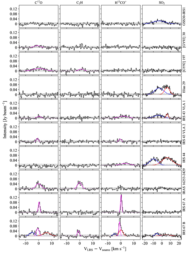
Figure 16: Spectra towards the source position; a Gaussian fit is overplotted (see Table 7). The blue, magenta, and red curves represent blue-shifted, quiescent, and red-shifted material, respectively. The dashed grey horizontal line shows the value of 3$\sigma$. All spectra have been shifted to the source velocity (see Table 4).