Electrical control and decoherence of the flopping-mode spin qubit

Electric-field control and noise protection of the flopping-mode spin qubit

Abstract

We propose and analyze a novel “flopping-mode” mechanism for electric dipole spin resonance based on the delocalization of a single electron across a double quantum dot confinement potential. Delocalization of the charge maximizes the electronic dipole moment compared to the conventional single dot spin resonance configuration. We present a theoretical investigation of the flopping-mode spin qubit properties through the crossover from the double to the single dot configuration by calculating effective spin Rabi frequencies and single-qubit gate fidelities. The flopping-mode regime optimizes the artificial spin-orbit effect generated by an external micromagnet and draws on the existence of an externally controllable sweet spot, where the coupling of the qubit to charge noise is highly suppressed. We further analyze the sweet spot behavior in the presence of a longitudinal magnetic field gradient, which gives rise to a second order sweet spot with reduced sensitivity to charge fluctuations.

I Introduction

Control of individual electron spins is one of the cornerstones of spin-based quantum technology. Although standard single-electron spin resonance has been demonstrated  Koppens et al. (2006), there is a strong incentive to avoid the use of local oscillating magnetic fields since these are technically demanding to generate at the nanoscale, hinder individual addressability, and limit the Rabi frequency due to sample heating issues. Electric dipole spin resonance (EDSR) techniques offer a more robust method to electrically control the electron spin state. Traditionally, successful implementations have used spin-orbit coupling  Nowack et al. (2007), hyperfine interaction Laird et al. (2007) and g-factor modulation  Kato et al. (2003).

The transition from GaAs to Si-based spin qubits has led to dramatic advances in the field of spin-based quantum computing. Site-selective single-qubit control Veldhorst et al. (2014); Takeda et al. (2016); Yoneda et al. (2018), two-qubit operations with high fidelity Veldhorst et al. (2015a); Zajac et al. (2016); Watson et al. (2018); Huang et al. (2019); Xue et al. (2019); Sigillito et al. (2019), electron shuttling Mills et al. (2019), and strong coupling to microwave photons Mi et al. (2018); Samkharadze et al. (2018) have been demonstrated. Recent demonstrations of strong spin-photon coupling have used double quantum dot (DQD) structures where the charge of one electron is delocalized between both dots (“flopping-mode”; Fig. 1(a)), thus enhancing the coupling strength to the cavity electric field beyond the decoherence rate  Mi et al. (2017); Stockklauser et al. (2017); Bruhat et al. (2018) and enabling the transfer of information between electron-spin qubits and microwave photons  Mi et al. (2018); Samkharadze et al. (2018); Cubaynes et al. . This suggests that the manipulation of electron spins with classical electric fields will also be efficient in the flopping-mode configuration.

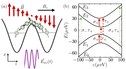
Figure 1: (a) Schematic illustration of the flopping-mode EDSR mechanism, where the spin of an electron (shown as green circles) delocalized between two QDs is driven via an electric field (purple line) in a magnetic field gradient (represented with red arrows). (b) Energy levels $E_{0,\dots,3}$ of the Hamiltonian (17) as a function of the interdot detuning $\varepsilon$, calculated with $t_{c}=20\,\mu\text{eV}$, $E_{z}=24\,\mu\text{eV}$, $g\mu_{B}b_{x}=15\,\mu\text{eV}$, and $g\mu_{B}b_{z}=4\,\mu\text{eV}$. The asymmetry with respect to $\varepsilon$ is due to the longitudinal magnetic field gradient. Around zero detuning, $|\varepsilon|\ll 2t_{c}$, the electron delocalizes across the DQD, yielding a larger electric dipole moment $p$ compared to the single dot regime. The arrows represent the electrically addressable spin (solid line), charge (dashed line) and spin-charge (dotted line) transitions.

The scalability of spin qubit processors hinges upon the use of resources that permit fast control without a significant degradation in coherence times. The same properties that make silicon based QDs extremely attractive for quantum information processing make it challenging to use its intrinsic properties for electrical spin manipulation. Not only is the hyperfine interaction to nuclear spins largely reduced, but the intrinsic spin-orbit coupling for electrons in Si is very weak Zwanenburg et al. (2013). Recently, this weak effect combined with the rich valley physics in Si has been harnessed to achieve EDSR for single-electron spin qubits  Veldhorst et al. (2015b); Corna et al. (2018) and singlet-triplet qubits Jock et al. (2018); Harvey-Collard et al. . A more flexible solution applicable to any semiconductor is the mixing of orbital motion and spin via an externally imposed magnetic field gradient  Pioro-Ladrière et al. (2008); Kawakami et al. (2014); Yoneda et al. (2018). Beyond this effective spin-orbit effect, the control over the magnetic field profile allows for selective addressing of spins placed in neighboring dots, since the resonance frequency varies spatially  Pioro-Ladrière et al. (2008); Obata et al. (2010); Nadj-Perge et al. (2010); Yoneda et al. (2014); Noiri et al. (2016); Takeda et al. (2016); Ito et al. (2018). Here we investigate the effect of the micromagnet stray field on the coherence of the flopping-mode spin qubit.

In this work we envision the generation of single-electron spin rotations via a flopping-mode approach, which benefits from the electron delocalization between two gate-defined tunnel coupled QDs Hu et al. (2012), and track its performance as the electron is spatially localized in a single quantum dot (SQD). The electron tunneling in such a double dot potential has a large electric dipole moment, which is partially transferred to the spin via the magnetic field gradient induced by the stray field of a micromagnet placed over the DQD, see Fig. 1(a). Moreover, due to the spatial separation between the two QDs, obtaining a sizable magnetic field inhomogeneity, with the resulting large effective spin orbit coupling, becomes relatively easy. A driving field on one of the gate electrodes that shapes the QD modulates the potential and allows full electrical spin control via EDSR.

The paper is organized as follows: In Sec. II we introduce the flopping-mode spin qubit and derive the Rabi frequency and the relevant relaxation and dephasing rates under the effect of a transverse magnetic field gradient for the case of zero energy level detuning. In Sec. III we take into account the effect of a general detuning and analyze the electrical control of the flopping-mode spin qubit as a function of externally controllable parameters. In Sec. IV we investigate the behavior of the flopping-mode spin qubit in the presence of a longitudinal magnetic field gradient and how this affects the working points with maximal single-qubit average gate fidelity. In Sec. V we summarize our results and conclude.

II Flopping-mode spin qubit

An electron trapped in a symmetric DQD, with zero energy level detuning $\epsilon=0$ between the left (L) and right (R) QDs will form bonding and antibonding charge states, which are separated by an energy $2t_{c}$, where $t_{c}$ is the interdot tunnel coupling. The transition dipole moment between the bonding and antibonding states, $|\mp\rangle=\left(|R\rangle\mp|L\rangle\right)/\sqrt{2}$, is proportional to the electronic charge $e$ and the distance between the two QDs $d$ Kim et al. (2015); Stockklauser et al. (2017); Bruhat et al. (2018); Mi et al. (2018), therefore an electric field with amplitude $E_{ac}$ at the position of the DQD can drive transitions with Rabi frequency $\Omega_{c}=edE_{ac}/\hbar$. Spins can be addressed via electric fields by splitting the spin states via a homogeneous magnetic field, $B_{z}$, and inducing an inhomogeneous magnetic field perpendicular to the spin quantization axis, i.e., transverse ($\pm b_{x}$ in the left/right QD). We model the spin and charge dynamics with the Hamiltonian

$$H_{0}^{\varepsilon=0}=t_{c}\tilde{\tau}_{z}+\frac{E_{z}}{2}\tilde{\sigma}_{z}-\frac{g\mu_{B}b_{x}}{2}\tilde{\sigma}_{x}\tilde{\tau}_{x}\ ,$$ (1)

where $\tilde{\tau}_{\alpha}$ and $\tilde{\sigma}_{\alpha}$ ($\alpha=x,y,z$) are the Pauli matrices in the charge ($|\pm\rangle$) and spin subspace, respectively, $E_{z}$ is the Zeeman energy $E_{z}=g\mu_{B}B_{z}$, $g$ is the electronic g-factor and $\mu_{B}$ the Bohr magneton. The magnetic field gradient acts as an artificial spin-orbit interaction and hybridizes bonding and antibonding states with opposite spin direction via the two spin-orbit mixing angles $\phi_{\pm}=\arctan{\left[g\mu_{B}b_{x}/(2t_{c}\pm E_{z})\right]}$ ($\phi_{\pm}\in[0,\pi]$). As a consequence of this mixing, the electric dipole moment operator acquires off-diagonal matrix elements in the eigenbasis of Eq. (1) which involve spin-flip transitions Benito et al. (2017, ). In particular, given the four eigenenergies $E_{0,\dots,3}$, with $2E_{3(2)}=-2E_{0(1)}=\sqrt{(2t_{c}\pm E_{z})^{2}+(g\mu_{B}b_{x})^{2}}$, if $\tau$ denotes the two-level-system with energy splitting $E_{\tau}=E_{2}-E_{0}$ and $\sigma$ the one with splitting $E_{\sigma}=E_{1}-E_{0}$ (see Fig. 1(b)), the electric dipole moment operator reads

$$p =ed\left[-\cos{\bar{\phi}}\tau_{x}+\sin{\bar{\phi}}\sigma_{x}\tau_{z}\right]\ ,$$ (2)

where $\bar{\phi}=\left(\phi_{+}+\phi_{-}\right)/2$, and $\tau(\sigma)_{\alpha}$ ($\alpha=x,y,z$) are the Pauli matrices in the corresponding $\tau(\sigma)$ subspace. This implies that the electric field can drive transitions between the ground state and the first and second excited states with Rabi frequency $\Omega_{\sigma}=\Omega_{c}\sin{\bar{\phi}}$ and $\Omega_{\tau}=\Omega_{c}\cos{\bar{\phi}}$, respectively; see the center part of Fig. 1(b), where we have defined $2\tau_{\pm}=\tau_{x}\pm i\tau_{y}$ and $2\sigma_{\pm}=\sigma_{x}\pm i\sigma_{y}$.

For $2t_{c}<E_{z}$ ($2t_{c}>E_{z}$), we define the spin qubit as $s=\tau$ ($s=\sigma$), i.e., as the ground state and the second (first) excited state, with Rabi frequency $\Omega_{s}=\Omega_{\tau}$ ($\Omega_{s}=\Omega_{\sigma}$). If the transverse magnetic field is small, $g\mu_{B}b_{x}\ll|2t_{c}-E_{z}|$, the expansion to first order yields

$$\Omega_{s}=2t_{c}g\mu_{B}b_{x}\Omega_{c}/|4t_{c}^{2}-E_{z}^{2}|+\mathcal{O}(b_{x}^{3})$$ (3)

for both $2t_{c}<E_{z}$ and $2t_{c}>E_{z}$. For a very small (or very large) tunnel splitting, $2t_{c}$, the qubit is an almost pure spin qubit and it is hardly addressable electrically, while in the region $2t_{c}\approx E_{z}$ the spin-electric field coupling is maximal Benito et al. (2017) but the spin qubit coherence suffers to some extent from charge noise (see below).

The spin or charge character of the qubit will be reflected in the decoherence time. The spin-charge mixing mechanism also couples the spin to the phonons in the host material, therefore the relaxation rates via phonon emission are $\gamma_{1,\sigma}=\gamma_{1,c}\sin^{2}(\bar{\phi})$ and $\gamma_{1,\tau}=\gamma_{1,c}\cos^{2}(\bar{\phi})$ Srinivasa et al. (2013), respectively, where we have introduced $\gamma_{1,c}$ as the relaxation rate from the antibonding to the bonding state evaluated at the qubit energy. Since the spin qubit energy is essentially given by the Zeeman splitting $E_{z}$ (weakly corrected by the spin-charge mixing), we can safely assume a constant value for $\gamma_{1,c}$, neglecting both oscillations of the form $\cos{(qd)}$ (q is the phonon quasimomentum) and polynomial dependences on the transition frequency Brandes and Kramer (1999); Tahan and Joynt (2014); Raith et al. (2011); Hu (2011); Kornich et al. (2018). The expansion to the lowest order in $b_{x}$ yields

$$\gamma_{1,s}=\gamma_{1,c}\left[2t_{c}g\mu_{B}b_{x}/(4t_{c}^{2}-E_{z}^{2})\right]^{2}+\mathcal{O}(b_{x}^{4})\ ,$$ (4)

where we can evaluate $\gamma_{1,c}$ at the Zeeman splitting energy $E_{z}$. In the symmetric configuration $\varepsilon=0$, pure dephasing is strongly suppressed since the qubit is in a sweet spot protected to some extent from charge fluctuations Vion et al. (2002); Petersson et al. (2010). Although the qubit energy splitting is first-order insensitive to electrical fluctuations in detuning $\varepsilon$, we account here for pure dephasing due to second-order coupling to charge fluctuations, which induces a Gaussian decay of coherences ($\propto e^{-(\gamma^{(2)}_{\phi,\sigma(\tau)}t)^{2}}$) with rates $\gamma^{(2)}_{\phi,\sigma}=(\gamma_{\phi}^{2}/E_{\sigma})\sin^{2}\bar{\phi}$ and $\gamma^{(2)}_{\phi,\tau}=(\gamma_{\phi}^{2}/E_{\tau})\cos^{2}\bar{\phi}$, where $\gamma_{\phi}$ is the magnitude of the low-frequency detuning charge fluctuations (see Appendix  A). The expansion to the lowest order in $b_{x}$ yields

$$\gamma_{\phi,s}^{(2)}=\frac{\gamma_{\phi}^{2}}{E_{z}}\left[2t_{c}g\mu_{B}b_{x}/(4t_{c}^{2}-E_{z}^{2})\right]^{2}+\mathcal{O}(b_{x}^{4})\ .$$ (5)

Note that far from the resonant point $2t_{c}\approx E_{z}$, other decoherence sources related to the spin, such as the hyperfine interaction with nuclear spins, would start dominating the dephasing. The dephasing corresponding to quasistatic magnetic noise Taylor et al. (2007); Chekhovich et al. (2013) with magnitude $\gamma_{M}$ is also quadratic, and the corresponding rates are $\gamma_{M,\sigma}=\gamma_{M}(\cos{\phi_{+}}+\cos{\phi_{-}})/2$ and $\gamma_{M,\tau}=\gamma_{M}(\cos{\phi_{+}}-\cos{\phi_{-}})/2$ (see Appendix B). Therefore, to lowest order in $b_{x}$, the spin qubit magnetic noise dephasing rate is

$$\gamma_{M,s}=\gamma_{M}\left[1-\frac{(g\mu_{B}b_{x})^{2}(4t_{c}^{2}+E_{z}^{2})}{2(4t_{c}^{2}-E_{z}^{2})^{2}}\right]+\mathcal{O}(b_{x}^{4})\ .$$ (6)

In this architecture the electric field can induce spin rotations with Rabi frequency $\Omega_{s}$. We focus on the shortest single-qubit spin rotation ($X_{\pi}$ gate), performed in the gate time $t_{g}=\pi/\Omega_{s}$. Using a master equation with qubit relaxation and a noise term, we calculate the average gate fidelity (see Appendix C) and average this result over a Gaussian distribution for the noise with standard deviation given by the total magnitude of the low-frequency noise, $\text{Var}(\delta)=2\left({\gamma_{\phi,s}^{(2)}}^{2}+\gamma_{M,s}^{2}\right)$. The optimal tunnel coupling value to achieve the best single-qubit average gate fidelity depends on the relation between the charge-induced dephasing and the magnetic noise (see Sec. III). Note that if the DQD is coupled to a microwave resonator the spin qubit couples also to the confined electric field and the Purcell effect opens another relaxation channel via photon emission. Single-spin control was demonstrated in Ref. Mi et al. (2018) in a detuned DQD configuration, where the spin-charge mixing, and therefore the coupling of the spin to the electric field is much weaker. In the following we analyze the crossover from a symmetric (DQD) to a far detuned (SQD) configuration.

III Crossover from DQD to SQD

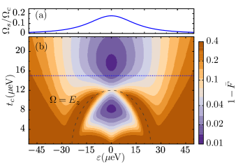
Figure 2: (a) Ratio between the spin Rabi frequency $\Omega_{s}$ and the charge Rabi frequency $\Omega_{c}$ as a function of detuning $\varepsilon$ for $t_{c}=15\,\mu\text{eV}$. The spin Rabi frequency is maximized for $\varepsilon=0$. (b) Single-qubit average gate infidelity as a function of $\varepsilon$ and $t_{c}$. As expected, $\bar{F}$ is symmetric about $\varepsilon=0$, with the highest values achieved at $\varepsilon=0$ and slightly away from the line with maximal spin-charge mixing, $\Omega=E_{z}$ (black dashed line). The other parameters are chosen to be $E_{z}=24\,\mu\text{eV}$, $g\mu_{B}b_{x}=2\,\mu\text{eV}$, $\Omega_{c}/2\pi=500\,\text{MHz}$, $\gamma_{1,c}/2\pi=18\,\text{MHz}$, $\gamma_{\phi}/2\pi=600\,\text{MHz}$, and $\gamma_{M}/2\pi=2\,\text{MHz}$.

In this section we calculate the spin Rabi frequency and the single-qubit average gate fidelity for a general detuning $\varepsilon$ and study the crossover from the molecular or DQD regime ($\varepsilon=0$) to the SQD regime with the electron strongly localized in the left or right QD ($|\varepsilon|\gg 2t_{c}$). An electron trapped in a detuned DQD, with energy detuning $\varepsilon$ between the left and the right QDs, forms charge states separated by an energy $\Omega=\sqrt{\varepsilon^{2}+4t_{c}^{2}}$. The detuning reduces the off-diagonal matrix elements of the transition dipole moment operator in the eigenbasis resulting in a Rabi frequency $\Omega^{\prime}_{c}=\Omega_{c}\cos{\theta}$, where we have introduced the orbital angle $\theta=\arctan{(\varepsilon/2t_{c})}$, and incorporates diagonal matrix elements. With a magnetic field profile as explained above, the model Hamiltonian reads Benito et al. (2017)

$$H_{0}=\frac{\Omega}{2}\tilde{\tau}_{z}+\frac{E_{z}}{2}\tilde{\sigma}_{z}-\frac{g\mu_{B}b_{x}\tilde{\sigma}_{x}}{2}\left(\cos{\theta}\tilde{\tau}_{x}-\sin{\theta}\tilde{\tau}_{z}\right)\ .$$ (7)

The eigenenergies, labelled as $E_{0,\dots,3}$ read $2E_{3(2)}=-2E_{0(1)}=\sqrt{\left(\Omega\pm b\right)^{2}+(g\mu_{B}b_{x}\cos\theta)^{2}}$, with $b=\sqrt{E_{z}^{2}+(g\mu_{B}b_{x}\sin\theta)^{2}}$, and all the off-diagonal matrix elements of the electric dipole moment operator in the eigenbasis are non-zero. Therefore all the transitions can be addressed electrically, as shown in Fig. 1(b) via colored arrows. The Rabi frequencies for the transitions involving the lower energy states are (see Appendix A) $\Omega_{\sigma}=\Omega^{\prime}_{c}\cos\Phi\sin\bar{\phi}$, and $\Omega_{\tau}=\Omega^{\prime}_{c}\cos\Phi\cos\bar{\phi}$, where the angle $\Phi=\arctan{\left(b_{x}\sin\theta/B_{z}\right)}$ describes an orbital-dependent spin rotation, $\phi_{\pm}=\arctan{\left[g\mu_{B}b_{x}\cos{\theta}/\left(\Omega\pm b\right)\right]}$ ($\phi_{\pm}\in[0,\pi]$) generalize the spin-orbit mixing angles, and $\bar{\phi}=\left(\phi_{+}+\phi_{-}\right)/2$.

Analogously to the previous section, we define the spin qubit as $s=\tau$ ($s=\sigma$) for $\Omega<E_{z}$ ($\Omega>E_{z}$), i.e., as the ground state and the second (first) excited state. As expected, the spin qubit Rabi frequency is reduced as $\varepsilon$ increases. The expansion of $\Omega_{s}$ for small $b_{x}$ ($g\mu_{B}b_{x}\ll|\Omega-E_{z}|$) yields

$$\Omega_{s}=2t_{c}g\mu_{B}b_{x}\Omega^{\prime}_{c}/|\Omega^{2}-E_{z}^{2}|+\mathcal{O}(b_{x}^{3})\ ,$$ (8)

generalizing Eq. (3) to $\varepsilon\neq 0$. In Fig. 2(a), we plot the ratio $\Omega_{s}/\Omega_{c}$ as a function of $\varepsilon$ for tunnel coupling $t_{c}=15\,\mu\text{eV}$ and fixed magnetic field profile, $E_{z}=24\,\mu\text{eV}$ and $g\mu_{B}b_{x}=2\,\mu\text{eV}$. As expected, for a given amplitude of the applied electric field the Rabi frequency is larger at zero detuning, which implies that at $\varepsilon\approx 0$ one can drive Rabi oscillations at a given frequency with less power consumption than for finite detuning; see Appendix D.

The direct phonon-induced spin relaxation rate for small $b_{x}$ reads

$$\gamma_{1,s}=\gamma_{1,c}(2t_{c}/\Omega)^{2}\left[2t_{c}g\mu_{B}b_{x}/(\Omega^{2}-E_{z}^{2})\right]^{2}+\mathcal{O}(b_{x}^{4})\ .$$ (9)

In this detuned situation, the second excited state can also decay to the first excited state via phonon emission, which opens another spin relaxation channel for the case $E_{z}>\Omega$ (see Appendix  A). However, the corresponding decay rate is lower than $\gamma_{1,c}$ due to the smaller energy gap between these two states and it can be neglected for the relevant parameters. Moreover the low-frequency charge fluctuations (with magnitude $\gamma_{\phi}$) induce pure dephasing with rates proportional to the first derivative of the transition frequencies with respect to $\varepsilon$,

$$\gamma_{\phi,\tau(\sigma)}^{(1)}=\frac{\gamma_{\phi}\cos{\theta}}{2} \left\{\tan{\theta}\left(\cos{\phi_{+}}\pm\cos{\phi_{-}}\right)\right.$$

$$\left.+\sin{\Phi}\left(\sin{\phi_{+}}\mp\sin{\phi_{-}}\right)\right\}$$ (10)

(see Appendix  A), which yields

$$\gamma_{\phi,s}^{(1)}=\frac{\gamma_{\phi}|\varepsilon|}{E_{z}}\left[2t_{c}g\mu_{B}b_{x}/(\Omega^{2}-E_{z}^{2})\right]^{2}+\mathcal{O}(b_{x}^{4})\,.$$ (11)

The second order contribution to spin dephasing is proportional to the second derivatives of the transition frequencies, as calculated from second order perturbation theory Cottet (2002); Chirolli and Burkard (2008); Russ and Burkard (2015). The full expression for this spin contribution is given in Appendix A. Including terms to lowest order in $b_{x}$, we find

$$\gamma_{\phi,s}^{(2)}=\frac{\gamma_{\phi}^{2}}{E_{z}}\left[\frac{2t_{c}g\mu_{B}b_{x}}{(\Omega^{2}-E_{z}^{2})}\right]^{2}\left[1-\frac{4\varepsilon^{2}}{\Omega^{2}-E_{z}^{2}}\right]+\mathcal{O}(b_{x}^{4})\ .$$ (12)

Finally, the dephasing rates corresponding to quasistatic magnetic noise are given in Appendix B and accounting for terms to lowest order in $b_{x}$, we find

$$\gamma_{M,s}=\gamma_{M} \frac{\sqrt{2\epsilon^{2}+4t_{c}^{2}}}{\Omega}\left[1-\frac{(g\mu_{B}b_{x}\varepsilon)^{2}}{2E_{z}^{2}\Omega^{2}}\right.$$

$$\left.-\frac{(g\mu_{B}b_{x})^{2}t_{c}^{2}(\Omega^{2}+E_{z}^{2})}{(2t_{c}^{2}+\epsilon^{2})(\Omega^{2}-E_{z}^{2})^{2}}\right]+\mathcal{O}(b_{x}^{4})\ .$$ (13)

In Fig. 2(b), we show the single-qubit average gate fidelity as a function of $\varepsilon$ and $t_{c}$, calculated by averaging the $X_{\pi}$ average gate fidelity in the presence of Gaussian distributed noise with standard deviation given by the total magnitude of the low-frequency noise, $\text{Var}(\delta)=2\left({\gamma_{\phi,s}^{(1)}}^{2}+{\gamma_{\phi,s}^{(2)}}^{2}+\gamma_{M,s}^{2}\right)$. First, we can observe the optimal values of $t_{c}$ mentioned in Sec. II and a reduction in the fidelity when $\Omega=E_{z}$ (indicated by the dashed line) due to large spin-charge mixing. Moreover, we can see the detrimental effect of working slightly away from the sweet spot ($\varepsilon=0$). The qubit not only suffers from a lower Rabi frequency but the first order charge noise contribution dominates, abruptly decreasing the average gate fidelity.

As an estimate of the number of Rabi oscillations that can be observed with high visibility in a EDSR experiment we can use the quality factor $Q$, defined as the ratio of spin Rabi frequency and decay rates

$$Q=\frac{2\Omega_{s}}{\gamma_{1,s}/2+\sqrt{{\gamma_{\phi,s}^{(1)}}^{2}+{\gamma_{\phi,s}^{(2)}}^{2}+\gamma_{M,s}^{2}}}\ .$$ (14)

This expression should be viewed as an approximate interpolation between the limiting cases where relaxation rate $\gamma_{1,s}$ or the low-frequency noise are dominating Croot et al. .

Increasing the detuning localizes the electron more in a single QD and the flopping-mode EDSR mechanism described above may compete with other EDSR mechanisms that take place in a SQD, via excited orbital or valley states Golovach et al. (2006); Tokura et al. (2006); Kawakami et al. (2014); Hao et al. (2014); Malkoc et al. (2016); Rančić and Burkard (2016); Corna et al. (2018); Bourdet and Niquet (2018). Also in a DQD structure, if the intervalley interdot tunnel coupling Burkard and Petta (2016); Huang et al. (2017); Mi et al. (2018) is strong compared to the valley splittings Mi et al. (2018), the effective spin Rabi frequency will be modified. In this work we focus on the micromagnet-induced flopping-mode EDSR mechanism, which dominates if the excited orbital and valley energy splittings are large enough. For a discussion of the interplay between micromagnet-induced SQD and flopping-mode EDSR mechanisms we refer the reader to Appendix D.

In more realistic setups, where the micromagnet stray field is not perfectly aligned with the DQD, there can be magnetic field gradients in the $z$ direction (longitudinal) and a finite average field in the $x$ direction (transverse). Given the importance of the protection against charge fluctuations, we investigate the sweet spot behavior using a more general model in the following section.

IV Flopping-mode charge noise sweet spots

In this section, we examine the optimal working points for flopping-mode spin qubit EDSR operation. For the model used in Sec. III, the zero detuning point constitutes a first order sweet spot with respect to fluctuations in the detuning, since the qubit energy is insensitive to $\varepsilon$ variations to first order. In this case, it is important to account for the second order contribution to qubit dephasing which, as mentioned above, is related to the second derivative of the qubit energy with respect to the detuning. The micromagnet could be designed to induce a longitudinal magnetic field gradient between the left and the right QDs with the aim of obtaining a different spin resonance frequency depending on the electron position. Fabrication misalignments can also give rise to both longitudinal gradients and overall transverse magnetic fields Samkharadze et al. (2018); Croot et al. ; Borjans et al. , i.e., the magnetic field components in the right and left QD positions may be $B^{(L,R)}_{z}=B_{z}\pm b_{z}$ and $B^{(L,R)}_{x}=B_{x}\pm b_{x}$, where $B_{z}\gg B_{x},b_{x},b_{z}$. Via a rotation of the spin quantization axis, given by the small angle $\zeta=\arctan{\left(B_{x}/B_{z}\right)}$, it is always possible to rewrite the latter as $B^{(L,R)}_{z^{\prime}}=\sqrt{B_{z}^{2}+B_{x}^{2}}\pm b_{z^{\prime}}$ and $B^{(L,R)}_{x^{\prime}}=\pm b_{x^{\prime}}$, with

$$b_{z^{\prime}} =b_{z}\cos\zeta+b_{x}\sin\zeta\ ,$$ (15)

$$b_{x^{\prime}} =b_{x}\cos\zeta-b_{z}\sin\zeta\ ,$$ (16)

therefore a model containing a homogeneous field and two gradients is sufficient. In the following we work in a rotated coordinate system and rename the variables as $\sqrt{B_{z}^{2}+B_{x}^{2}}\rightarrow B_{z}$, $b_{x^{\prime}}\rightarrow b_{x}$ and $b_{z^{\prime}}\rightarrow b_{z}$. This allows us to use the model Hamiltonian in Eq. (7), with a homogeneous field $B_{z}$ and a transverse inhomogeneous component $b_{x}$, and add a term accounting for the longitudinal gradient ($\pm b_{z}$ in the left/right QD),

$$H=H_{0}-\frac{g\mu_{B}b_{z}\tilde{\sigma}_{z}}{2}\left(\cos{\theta}\tilde{\tau}_{x}-\sin{\theta}\tilde{\tau}_{z}\right)\ .$$ (17)

Note that the relative values of $b_{x}$ and $b_{z}$ can be controlled via the direction of the external magnetic field Borjans et al. .

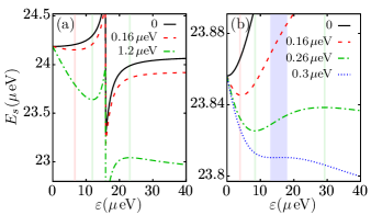
Figure 3: Spin qubit energy splitting $E_{s}$ as a function of the detuning $\varepsilon$, for various values of the longitudinal gradient field ($g\mu_{B}b_{z}$), as indicated, increasing from top to bottom. The interdot tunnel splitting amounts to (a) $2t_{c}=18\,\mu\text{eV}$ and (b) $2t_{c}=30\,\mu\text{eV}$, while the homogeneous field Zeeman energy is $E_{z}=24\,\mu\text{eV}$ and the transverse inhomogeneous component is $g\mu_{B}b_{x}=2\,\mu\text{eV}$. The thin shaded areas indicate first order sweet spots for the corresponding color line and the wide blue shaded area in (b) indicates the region around the second order sweet spot for $g\mu_{B}b_{z}=0.3\,\mu\text{eV}$. The discontinuity in (a) occurs at $\Omega=E_{z}$ due to a level crossing of the upper qubit state.

For simplicity we analyze first this model in the limit of small inhomogeneous fields, $g\mu_{B}b_{x,z}\ll|\Omega-E_{z}|$. While the transverse gradient corrects the spin qubit energy splitting $E_{s}$ (from the value $E_{s}=E_{z}$ for $b_{x,z}=0$) to second order, the longitudinal gradient has an effect to first order, leading to

$$E_{s}\simeq E_{z}-\frac{E_{z}^{2}-\varepsilon^{2}}{2E_{z}(\Omega^{2}-E_{z}^{2})}(g\mu_{B}b_{x})^{2}-\frac{\varepsilon}{\Omega}g\mu_{B}b_{z}\ .$$ (18)

From this simplified expression, we can explore the existence of first order sweet spots. Unless $b_{z}=0$, the spin qubit does not have a first order sweet spot at zero detuning. For an arbitrary value of $t_{c}$, if $b_{z}<b_{x}^{2}/B_{z}$ the spin qubit should be operated at a first order sweet spot slightly shifted from zero detuning (see below). For a larger longitudinal gradient, $b_{z}>b_{x}^{2}/B_{z}$, there are two first order sweet spots for a given value of tunnel splitting below the Zeeman energy, i.e., $2t_{c}<E_{z}$. For larger tunnel splitting, $2E_{z}>2t_{c}>E_{z}$, there are also two first order sweet spots if

$$\frac{b_{x}^{2}}{B_{z}}<b_{z}<b_{z}^{0}=\frac{3\sqrt{3}t_{c}^{4}}{E_{z}(4t_{c}^{2}-E_{z}^{2})^{3/2}}\frac{b_{x}^{2}}{B_{z}}$$ (19)

and none otherwise.

In Fig. 3, the exact spin qubit energy splitting $E_{s}$, calculated from the eigenenergies of the Hamiltonian (17), is shown as a function of the DQD detuning $\varepsilon$ for different values of $b_{z}$. For negative values of $b_{z}$ the sweet spots will occur at negative values of $\varepsilon$. The panels (a) and (b) represent a generic case with tunnel splitting below and above the Zeeman energy, respectively. The black (solid) lines are for $b_{z}=0$ and the red (dashed) lines correspond to $b_{z}<b_{x}^{2}/B_{z}$, showing therefore one first order sweet spot in both panels (a) and (b). In Fig. 3(a), since $2t_{c}<E_{z}$, we expect two first order sweet spots for large enough values of longitudinal gradient, which can be seen in the green (dash-dotted) line. In Fig. 3(b), we analyze a case with $2E_{z}>2t_{c}>E_{z}$. The green (dash-dotted) line corresponds to the intermediate region of two first order sweet spots, $b_{x}^{2}/B_{z}<b_{z}<b_{z}^{0}$. Finally, the blue (dotted) line is obtained for $b_{z}\sim b_{z}^{0}$. At this point, $E_{s}$ becomes very flat, which would protect the qubit even to higher order from fluctuations in the detuning.

To confirm this, we show in Fig. 4 the second derivative of the spin qubit energy splitting with respect to detuning. In panel (a) $b_{z}<b_{x}^{2}/B_{z}$, while in panel (b) $b_{z}>b_{x}^{2}/B_{z}$. The superimposed black dashed line indicates the position of the first order sweet spots. In Fig. 4(a), the value of the second derivative along the expected first order sweet spot (black dashed line) does not change significantly. Increasing the value of $b_{z}$ can give rise to a situation as shown in Fig. 4(b), where the line indicating the position of the first order sweet spot (black dashed line) crosses the line of zero second derivative, allowing for a second order sweet spot and a qubit protected against charge noise up to second order.

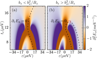
Figure 4: Second derivative $\partial^{2}_{\varepsilon}E_{s}$ of the spin qubit energy splitting with respect to the detuning $\varepsilon$ as a function of $t_{c}$ and $\varepsilon$ for (a) $g\mu_{B}b_{z}=0.16\,\mu\text{eV}$ and (b) $g\mu_{B}b_{z}=0.5\,\mu\text{eV}$. The black dashed lines indicate the first order sweet spot positions and the circle in panel (b) indicates the position of the second order sweet spot. The homogeneous field Zeeman energy is $E_{z}=24\,\mu\text{eV}$ and the transverse inhomogeneous component is $g\mu_{B}b_{x}=2\,\mu\text{eV}$.

The longitudinal magnetic field gradient may also influence the electric dipole moment operator and therefore the Rabi frequencies of the different transitions. In Appendix E we treat the transverse component $b_{x}$ perturbatively and calculate the correction of the spin Rabi frequency due to the longitudinal magnetic field gradient,

$$\Omega_{s}\simeq\Omega^{\prime}_{c}\frac{2t_{c}g\mu_{B}b_{x}}{|\Omega^{2}-E_{z}^{2}|}\left[1+\frac{\varepsilon b_{z}}{\Omega B_{z}}\right]\ ,$$ (20)

i.e., $b_{z}\ll B_{z}$ incorporates a small correction. This means that $b_{z}$ does not have a noticeable effect on the spin Rabi frequency and the phonon induced spin dephasing rate, but it strongly affects the pure spin dephasing rate due to charge fluctuations via a drastic modification of the qubit energy detuning dependence, as shown in Figs. 3 and 4.

To examine the overall performance of the qubit in different regimes, we show in Fig. 5 the single-qubit average gate fidelity as a function of $\varepsilon$ and $t_{c}$. The charge noise induced spin dephasing rate has been calculated numerically from the derivatives of the spin qubit energy splitting $E_{s}$ with respect to detuning $\varepsilon$. The effect of the small longitudinal gradient on the spin Rabi frequency, the phonon induced spin relaxation rate and the magnetic noise induced rate is very small, therefore we have neglected it here. Since we have assumed that the pure dephasing rate induced by charge noise fluctuations is the dominant source of decoherence, the condition for the best quality qubit coincides with the position of the first order sweet spots, which, as opposed to the case with $b_{z}=0$ shown in Fig. 2, does not occur at $\varepsilon=0$. Although for a fixed tunnel coupling $t_{c}$ the two first order sweet spots exhibit high single-qubit average gate fidelity, their properties are very different. For example, for $t_{c}=13\,\mu\text{eV}$ the spin Rabi frequency at the sweet spot at $\epsilon=3.1\,\mu\text{eV}$ is four times larger than at the one at $\epsilon=18.6\,\mu\text{eV}$ (these two first-order sweet spots are indicated by squares in Fig. 5(b)), but the phonon-induced relaxation rate and the charge noise dephasing rates are also 16 and 9 times higher, respectively. The first order sweet spot situated at larger detuning could therefore serve as idle point, while the one at lower detuning is used as operating point. Finally, as shown in Fig. 5(b), an even larger average gate fidelity can be achieved by operating close to the second order sweet spot. Note that the best fidelity does not correspond exactly to the second order sweet spot, since phonon relaxation and nuclear spin induced dephasing are also present.

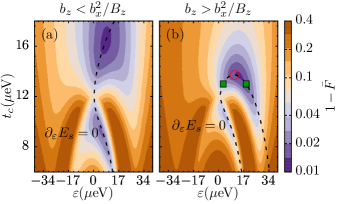
Figure 5: Single-qubit average gate infidelity $1-\bar{F}$ as a function of detuning $\varepsilon$ and interdot tunnel coupling $t_{c}$ for (a) $g\mu_{B}b_{z}=0.16\,\mu\text{eV}$ and (b) $g\mu_{B}b_{z}=0.5\,\mu\text{eV}$. The homogeneous field Zeeman energy is $E_{z}=24\,\mu\text{eV}$ and the transverse inhomogeneous component is $g\mu_{B}b_{x}=2\,\mu\text{eV}$. The other parameters are chosen to be $\Omega_{c}/2\pi=500\,\text{MHz}$, $\gamma_{1,c}/2\pi=18\,\text{MHz}$, $\gamma_{\phi}/2\pi=600\,\text{MHz}$, and $\gamma_{M}/2\pi=2\,\text{MHz}$. The black dashed lines indicate the first order sweet spot positions. In panel (b) the squares mark the position of the first order sweet spots for $t_{c}=13\,\mu\text{eV}$ and the circle indicates the position of the second order sweet spot.

V Conclusions

The flopping-mode configuration is shown to be useful not only for achieving a strong coupling between cavity photons and single spins  Mi et al. (2018); Samkharadze et al. (2018); Cubaynes et al. , but also for coherent electrical spin manipulation. We have analyzed the variation of the performance of the flopping-mode EDSR method from the symmetric ($\varepsilon=0$) DQD to the highly biased ($|\varepsilon|\gg 2t_{c}$) SQD regime. Importantly, the applied power of the electric field necessary to obtain a given Rabi frequency will be reduced by orders of magnitude by working in the DQD regime. This efficient single spin manipulation implemented in silicon QDs would constitute a fundamental step towards a fully electrically controllable quantum processing architecture for spin qubits, a platform which already benefits from mature silicon processing technology.

Given the presence of environmental charge noise in typical QD devices, it is important to know the position of the exact first order sweet spot, which can be shifted a few $\mu$eVs away from zero detuning in the presence of a longitudinal magnetic field gradient. Interestingly, it is also possible to find two first order sweet spots for the same value of tunnel coupling, with different Rabi frequency and decoherence rate, which could be potentially exploited for different steps of qubit manipulation. Finally, we predict the existence of second order sweet spots, where the qubit is insensitive to electrical fluctuations up to second order.

Appendix A Electric dipole moment and dephasing

In this Appendix we calculate the Rabi frequencies for the different transitions in the flopping-mode spin qubit, the phonon-induced spin relaxation rates and the pure dephasing rates due to low-frequency electrical fluctuations in the DQD detuning. In Eq. (2) we have expressed the electric dipole moment operator in the eigenbasis of Eq. (1), which is the model Hamiltonian for $\varepsilon=0$ and $b_{z}=0$. For detuned QDs ($\varepsilon\neq 0$), we can write the electric dipole moment in the eigenbasis of the Hamiltonian in Eq. (7) and find that the electric field couples to all possible electronic transitions, as shown in Fig. 1(b), since the electric dipole moment operator has the form $p=ed\cos{\theta}(\mathcal{T}+\mathcal{Z}/2)$, with the off-diagonal component

$$\mathcal{T}= -\cos{\Phi}\cos{\bar{\phi}}\tau_{x}+\cos{\Phi}\sin{\bar{\phi}}\sigma_{x}\tau_{z}$$ (21)

$$+\left(\sin{\Phi}\cos{\phi_{-}}+\tan{\theta}\sin{\phi_{-}}\right)(\sigma_{+}\tau_{-}+h.c.)$$

$$-\left(\sin{\Phi}\cos{\phi_{+}}-\tan{\theta}\sin{\phi_{+}}\right)(\sigma_{+}\tau_{+}+h.c.)\ ,$$

and the diagonal component

$$\mathcal{Z}= \left\{\tan{\theta}\left(\cos{\phi_{+}}+\cos{\phi_{-}}\right)\right.$$

$$\left.+\sin{\Phi}\left(\sin{\phi_{+}}-\sin{\phi_{-}}\right)\right\}\tau_{z}$$

$$+ \left\{\tan{\theta}\left(\cos{\phi_{+}}-\cos\phi_{-}\right)\right.$$

$$\left.+\sin{\Phi}\left(\sin{\phi_{+}}+\sin{\phi_{-}}\right)\right\}\sigma_{z}\ .$$ (22)

The first terms in the off-diagonal component determine the Rabi frequencies $\Omega_{\tau(\sigma)}$ and the direct phonon relaxation rates $\gamma_{1,\tau(\sigma)}$ given in Sec. III. The term in the second line of Eq. (21) corresponds to transitions between the first and second excited states, and it opens a new channel for spin relaxation in the case $E_{z}>\Omega$. We have neglected this channel here because the corresponding phonon emission rate is suppressed by the small energy gap between these two states for the relevant parameter regimes.

The electrical fluctuations also couple to the system via the electric dipole moment. If the amplitude $\delta_{\varepsilon}$ and frequency of these fluctuations is small, we can calculate the spin qubit dephasing rate by treating them within time-independent perturbation theory Cottet (2002); Chirolli and Burkard (2008); Russ and Burkard (2015), obtaining the dephasing Hamiltonian

$$H_{\delta_{\varepsilon}}=\sum_{\eta=\tau,\sigma}\left(\frac{\partial E_{\eta}}{\partial\varepsilon}\delta_{\varepsilon}+\frac{1}{2}\frac{\partial^{2}E_{\eta}}{\partial\varepsilon^{2}}\delta_{\varepsilon}^{2}\right)\frac{\eta_{z}}{2}\ ,$$ (23)

where the first order contribution relates directly to the diagonal components in Eq. (22), since

$$\frac{\partial E_{\tau(\sigma)}}{\partial\varepsilon}=\frac{\cos{\theta}}{2} \left\{\tan{\theta}\left(\cos{\phi_{+}}\pm\cos{\phi_{-}}\right)\right.$$

$$\left.+\sin{\Phi}\left(\sin{\phi_{+}}\mp\sin{\phi_{-}}\right)\right\}\ .$$ (24)

and all the terms of the off-diagonal component Eq. (21) contribute to second order Russ and Burkard (2015). More precisely, the second derivatives read

$$\frac{\partial^{2}E_{\tau(\sigma)}}{\partial\varepsilon^{2}} =\cos^{2}{\theta}\left\{\frac{\cos^{2}{\Phi}\cos^{2}{\bar{\phi}}}{E_{\tau(\sigma)}}\right.$$

$$\left.+\frac{\left(\sin{\Phi}\cos{\phi_{+}}-\tan{\theta}\sin{\phi_{+}}\right)^{2}}{2(E_{\tau}+E_{\sigma})}\right.$$

$$\left.\pm\frac{\left(\sin{\Phi}\cos{\phi_{-}}+\tan{\theta}\sin{\phi_{-}}\right)^{2}}{2(E_{\tau}-E_{\sigma})}\right\}\ .$$ (25)

Assuming Gaussian distributed low frequency noise leads to a Gaussian decay of coherence $\propto e^{-\Gamma_{\phi}^{2}t^{2}}$ with the total pure spin dephasing rate related to the variance of the noise function

$$\Gamma_{\phi} =\left[\text{Var}\left(\frac{\partial E_{s}}{\partial\varepsilon}\delta_{\varepsilon}+\frac{1}{2}\frac{\partial^{2}E_{s}}{\partial\varepsilon^{2}}\delta_{\varepsilon}^{2}\right)/2\right]^{1/2}$$

$$=\left[{\gamma_{\phi,s}^{(1)}}^{2}+{\gamma_{\phi,s}^{(2)}}^{2}\right]^{1/2}\ ,$$ (26)

where $\gamma_{\phi,s}^{(1)}=\gamma_{\phi}\frac{\partial_{\varepsilon}E_{s}}{\partial\varepsilon}$, $\gamma_{\phi,s}^{(2)}=\gamma_{\phi}^{2}\frac{\partial_{\varepsilon}^{2}E_{s}}{\partial\varepsilon^{2}}$, and $\gamma_{\phi}=\sigma_{\varepsilon}/\sqrt{2}$, where $\sigma_{\varepsilon}$ is the standard deviation of the fluctuations $\delta_{\varepsilon}$.

Appendix B Quasistatic magnetic noise

In this Appendix we calculate the dephasing rate of the flopping-mode spin qubit due to hyperfine interaction with the nuclear spins. For this we use the quasistatic approximation Taylor et al. (2007), which assumes that the fluctuations in the Overhauser field occur in a time scale much longer than the system dynamics. Then we treat the noise Hamiltonian term

$$\tilde{V}=\xi_{L}(t)\tilde{\sigma}_{z}(1+\tilde{\tau}_{z})/2+\xi_{R}(t)\tilde{\sigma}_{z}(1-\tilde{\tau}_{z})/2\ ,$$ (27)

with two random variables for the noise in the left and right QDs, to first order in time-independent perturbation theory. First we transform Eq. (27) into the eigenbasis of Eq. (7), obtaining the diagonal component

$$\mathcal{Z}=\frac{\xi_{+}\cos{\Phi}}{4}\left\{\left(\cos\phi_{+}-\cos\phi_{-}\right)\tau_{z}\right.$$

$$\left.+\left(\cos\phi_{+}+\cos\phi_{-}\right)\sigma_{z}\right\}$$

$$+\frac{\xi_{-}\cos{\Phi}\sin\theta}{2}\sigma_{z}\tau_{z} \ ,$$ (28)

where $\xi_{\pm}=\xi_{L}(t)\pm\xi_{R}(t)$.

If we assume now Gaussian distributions with zero mean value and $\sigma_{M}^{2}=\text{Var}\left(\xi_{R}(t)\right)=\text{Var}\left(\xi_{L}(t)\right)$, the coherences decay as $\propto e^{-(\gamma_{M,\sigma(\tau)}t)^{2}}$, with the dephasing rates due to nuclear spins

$$\gamma_{M,\sigma(\tau)}=\frac{\gamma_{M}\cos{\Phi}}{2}\sqrt{\left(\cos\phi_{+}\pm\cos\phi_{-}\right)^{2}+4\sin^{2}\theta}\ ,$$ (29)

where $\gamma_{M}=\sigma_{M}$, whose expansion to lowest order in $b_{x}$ yields Eq. (13).

Appendix C Single-qubit average gate fidelity

We determine the quality of the quantum gate, represented by the operator $\cal{E}$, via the average fidelity $\bar{F}=\overline{\langle\psi|\cal{E}[|\psi_{\rm i}\rangle]|\psi\rangle}$, which compares the targeted pure state $\ket{\psi}$ and the obtained mixed state density matrix $\cal{E}[|\psi_{\rm i}\rangle]$, averaged over all possible pure input states $|\psi_{\rm i}\rangle$. In this case the real quantum gate is determined by the simple two-level system master equation

$$\dot{\rho}=-i\left[\frac{\delta}{2}\sigma_{z},\rho\right]+\frac{\gamma_{1,s}}{2}\left[2\sigma_{-}\rho\sigma_{+}-\left\{\sigma_{+}\sigma_{-},\rho\right\}\right]$$ (30)

for the qubit density matrix $\rho$, where $\delta$ is the noise magnitude.

We now calculate the entanglement fidelity $F_{e}$ for the gate applied to only one qubit of a two-qubit state prepared in a maximally entangled state, since this relates to the average fidelity as $\bar{F}=(2F_{e}+1)/3$ Horodecki et al. (1999). This yields

$$\bar{F}(\delta) =\frac{1}{3}\left\{2+e^{-2t_{g}\gamma_{1,s}}\right.$$ (31)

$$\left.+e^{-t_{g}\gamma_{1,s}}\left[\cosh{\left(t_{g}\gamma_{1,s}\right)}-\cosh{\left(t_{g}\sqrt{\gamma_{1,s}^{2}-\delta^{2}}\right)}\right]\right\}\ .$$

Finally, since we consider only low-frequency noise, the measurable and interesting quantity is the average of this fidelity over the randomly distributed noise variable $\delta$.

Appendix D Low power EDSR

In this Appendix, we analyze the power necessary to drive Rabi oscillations at a given frequency by taking into account both SQD and flopping-mode EDSR induced by the micromagnet. Following Refs. Pioro-Ladrière et al. (2008); Kawakami et al. (2014), we can complete Eq. (8) by including the SQD contribution to the Rabi frequency,

$$\Omega_{s}\approx\frac{edE_{ac}}{\hbar}g\mu_{B}b_{x}\left(\frac{4t_{c}^{2}}{\Omega|\Omega^{2}-E_{z}^{2}|}+\frac{\hbar^{2}}{m_{e}^{*}d^{2}E^{2}_{\text{orb}}}\right)\ ,$$ (32)

where $E_{\text{orb}}$ is the orbital energy, $E_{\text{orb}}\approx 1-3\,\text{meV}$, and $m_{e}^{*}$ is the electron effective mass. Since the drive power is proportional to the square of the electric field, $P\propto E_{ac}^{2}$, the power necessary to drive the spin qubit at a given Rabi frequency follows Croot et al.

$$P\propto\Omega_{s}^{2}\left[\frac{ed}{\hbar}g\mu_{B}b_{x}\left(\frac{4t_{c}^{2}}{\Omega|\Omega^{2}-E_{z}^{2}|}+\frac{\hbar^{2}}{m_{e}^{*}d^{2}E^{2}_{\text{orb}}}\right)\right]^{-2}\ .$$ (33)

Appendix E Effect of $b_{z}$ on the spin Rabi frequency

In this Appendix we investigate the effect of a longitudinal magnetic field gradient on the flopping-mode Rabi frequencies. Since $b_{z}$ is the difference in longitudinal magnetic field between the left and the right QDs, it can be seen as a detuning parameter (similar to $\varepsilon$) that depends on the spin, therefore its effect can be included in the form of a spin-dependent orbital basis transformation,

$$|+^{\prime},\sigma\rangle= \cos{(\theta_{\sigma}/2)}|+,\sigma\rangle-\sin{(\theta_{\sigma}/2)}|-,\sigma\rangle\ ,$$

$$|-^{\prime},\sigma\rangle= \sin{(\theta_{\sigma}/2)}|+,\sigma\rangle+\cos{(\theta_{\sigma}/2)}|-,\sigma\rangle\ ,$$ (34)

with orbital angles $\theta_{\uparrow(\downarrow)}=\arctan{\left[(\varepsilon\pm g\mu_{B}b_{z})/2t_{c}\right]}$ and orbital energies $\Omega_{\uparrow(\downarrow)}=\sqrt{(\varepsilon\pm g\mu_{B}b_{z})^{2}+4t_{c}^{2}}$, instead of the $\theta$ and $\Omega$ used in Sec. III. With this, we can treat $b_{x}$ perturbatively and find the spin Rabi frequency

$$\Omega_{s}\simeq 2t_{c}g\mu_{B}b_{x}\Omega_{c}\cos{\bar{\theta}}\frac{E_{z}/\left[E_{z}-(\Omega_{\uparrow}-\Omega_{\downarrow})/2\right]}{(\Omega_{\uparrow}+\Omega_{\downarrow})^{2}/4-E_{z}^{2}}\ ,$$ (35)

that generalizes the result in Eq. (8). Here, $\bar{\theta}=(\theta_{\uparrow}+\theta_{\downarrow})/2$. Finally, expanding to lowest order in $b_{z}$, this simplifies to Eq. (20).

References

- Koppens et al. (2006) F. H. L. Koppens, C. Buizert, K. J. Tielrooij, I. T. Vink, K. C. Nowack, T. Meunier, L. P. Kouwenhoven, and L. M. K. Vandersypen, “Driven coherent oscillations of a single electron spin in a quantum dot,” Nature 442, 766 (2006).
- Nowack et al. (2007) K. C. Nowack, F. H. L. Koppens, Yu. V. Nazarov, and L. M. K. Vandersypen, “Coherent control of a single electron spin with electric fields,” Science 318, 1430 (2007).
- Laird et al. (2007) E. A. Laird, C. Barthel, E. I. Rashba, C. M. Marcus, M. P. Hanson, and A. C. Gossard, “Hyperfine-mediated gate-driven electron spin resonance,” Phys. Rev. Lett. 99, 246601 (2007).
- Kato et al. (2003) Y. Kato, R. C. Myers, D. C. Driscoll, A. C. Gossard, J. Levy, and D. D. Awschalom, “Gigahertz electron spin manipulation using voltage-controlled g-tensor modulation,” Science 299, 1201 (2003).
- Veldhorst et al. (2014) M. Veldhorst, J. C. C. Hwang, C. H. Yang, A. W. Leenstra, B. de Ronde, J. P. Dehollain, J. T. Muhonen, F. E. Hudson, K. M. Itoh, A. Morello, and A. S. Dzurak, “An addressable quantum dot qubit with fault-tolerant control-fidelity,” Nat. Nanotechnol. 9, 981 (2014).
- Takeda et al. (2016) K. Takeda, J. Kamioka, T. Otsuka, J. Yoneda, T. Nakajima, M. R. Delbecq, S. Amaha, G. Allison, T. Kodera, S. Oda, and S. Tarucha, “A fault-tolerant addressable spin qubit in a natural silicon quantum dot,” Sci. Adv. 2, e1600694 (2016).
- Yoneda et al. (2018) J. Yoneda, K. Takeda, T. Otsuka, T. Nakajima, M. R. Delbecq, G. Allison, T. Honda, T. Kodera, S. Oda, Y. Hoshi, N. Usami, K. M. Itoh, and S. Tarucha, “A quantum-dot spin qubit with coherence limited by charge noise and fidelity higher than 99.9%,” Nat. Nanotechnol. 13, 102 (2018).
- Veldhorst et al. (2015a) M. Veldhorst, C. H. Yang, J. C. C. Hwang, W. Huang, J. P. Dehollain, J. T. Muhonen, S. Simmons, A. Laucht, F. E. Hudson, K. M. Itoh, A. Morello, and A. S. Dzurak, “A two-qubit logic gate in silicon,” Nature 526, 410 (2015a).
- Zajac et al. (2016) D. M. Zajac, T. M. Hazard, X. Mi, E. Nielsen, and J. R. Petta, “Scalable gate architecture for a one-dimensional array of semiconductor spin qubits,” Phys. Rev. Appl. 6, 054013 (2016).
- Watson et al. (2018) T. F. Watson, S. G. J. Philips, D. R. Kawakami, E. Ward, P. Scarlino, M. Veldhorst, D. E. Savage, M. G. Lagally, Mark Friesen, S. N. Coppersmith, M. A. Eriksson, and L. M. K. Vandersypen, “A programmable two-qubit quantum processor in silicon,” Nature 555, 633 (2018).
- Huang et al. (2019) W. Huang, C. H. Yang, K. W. Chan, T. Tanttu, B. Hensen, R. C. C. Leon, M. A. Fogarty, J. C. C. Hwang, F. E. Hudson, K. M. Itoh, A. Morello, A. Laucht, and A. S. Dzurak, “Fidelity benchmarks for two-qubit gates in silicon,” Nature 569, 532 (2019).
- Xue et al. (2019) X. Xue, T. F. Watson, J. Helsen, D. R. Ward, D. E. Savage, M. G. Lagally, S. N. Coppersmith, M. A. Eriksson, S. Wehner, and L. M. K. Vandersypen, “Benchmarking gate fidelities in a two-qubit device,” Phys. Rev. X 9, 021011 (2019).
- Sigillito et al. (2019) A.J. Sigillito, J.C. Loy, D.M. Zajac, M.J. Gullans, L.F. Edge, and J.R. Petta, “Site-selective quantum control in an isotopically enriched quadruple quantum dot,” Phys. Rev. Applied 11, 061006 (2019).
- Mills et al. (2019) A. R. Mills, D. M. Zajac, M. J. Gullans, F. J. Schupp, T. M. Hazard, and J. R. Petta, “Shuttling a single charge across a one-dimensional array of silicon quantum dots,” Nat. Commun. 10, 1063 (2019).
- Mi et al. (2018) X. Mi, M. Benito, S. Putz, D. M. Zajac, J. M. Taylor, G. Burkard, and J. R. Petta, “A coherent spin-photon interface in silicon,” Nature 555, 599 (2018).
- Samkharadze et al. (2018) N. Samkharadze, G. Zheng, N. Kalhor, D. Brousse, A. Sammak, U. C. Mendes, A. Blais, G. Scappucci, and L. M. K. Vandersypen, “Strong spin-photon coupling in silicon,” Science 359, 1123 (2018).
- Mi et al. (2017) X. Mi, J. V. Cady, D. M. Zajac, P. W. Deelman, and J. R. Petta, “Strong coupling of a single electron in silicon to a microwave photon,” Science 335, 156 (2017).
- Stockklauser et al. (2017) A. Stockklauser, P. Scarlino, J. V. Koski, S. Gasparinetti, C. K. Andersen, C. Reichl, W. Wegscheider, T. Ihn, K. Ensslin, and A. Wallraff, “Strong coupling cavity QED with gate-defined double quantum dots enabled by a high impedance resonator,” Phys. Rev. X 7, 011030 (2017).
- Bruhat et al. (2018) L. E. Bruhat, T. Cubaynes, J. J. Viennot, M. C. Dartiailh, M. M. Desjardins, A. Cottet, and T. Kontos, “Circuit QED with a quantum-dot charge qubit dressed by cooper pairs,” Phys. Rev. B 98, 155313 (2018).
- (20) T. Cubaynes, M. R. Delbecq, M. C. Dartiailh, R. Assouly, M. M. Desjardins, L. C. Contamin, L. E. Bruhat, Z. Leghtas, F. Mallet, A. Cottet, and T. Kontos, “Highly coherent spin states in carbon nanotubes coupled to cavity photons,” arXiv:1903.05229 .
- Zwanenburg et al. (2013) F. A. Zwanenburg, A. S. Dzurak, A. Morello, M. Y. Simmons, L. C. L. Hollenberg, G. Klimeck, S. Rogge, S. N. Coppersmith, and M. A. Eriksson, “Silicon quantum electronics,” Rev. Mod. Phys. 85, 961 (2013).
- Veldhorst et al. (2015b) M. Veldhorst, R. Ruskov, C. H. Yang, J. C. C. Hwang, F. E. Hudson, M. E. Flatté, C. Tahan, K. M. Itoh, A. Morello, and A. S. Dzurak, “Spin-orbit coupling and operation of multivalley spin qubits,” Phys. Rev. B 92, 201401 (2015b).
- Corna et al. (2018) A. Corna, L. Bourdet, R. Maurand, A. Crippa, D. Kotekar-Patil, H. Bohuslavskyi, R. Laviéville, L. Hutin, S. Barraud, X. Jehl, M. Vinet, S. de Franceschi, Y-M. Niquet, and M. Sanquer, “Electrically driven electron spin resonance mediated by spin-valley-orbit coupling in a silicon quantum dot,” npj Quantum Inf. 4, 6 (2018).
- Jock et al. (2018) R. M. Jock, N. T. Jacobson, P. Harvey-Collard, A. M. Mounce, V. Srinivasa, D. R. Ward, J. Anderson, R. Manginell, J. R. Wendt, M. Rudolph, T. Pluym, J. K. Gamble, A. D. Baczewski, W. M. Witzel, and M. S. Carroll, “A silicon metal-oxide-semiconductor electron spin-orbit qubit,” Nat. Commun. 9, 1768 (2018).
- (25) P. Harvey-Collard, N. T. Jacobson, C. Bureau-Oxton, R. M. Jock, V. Srinivasa, A. M. Mounce, D. R. Ward, J. M. Anderson, R. P. Manginell, J. R. Wendt, T. Pluym, M. P. Lilly, D. R. Luhman, M. Pioro-Ladrière, and M. S. Carroll, “Implications of the spin-orbit interaction for singlet-triplet qubits in silicon,” arXiv:1808.07378 .
- Pioro-Ladrière et al. (2008) M. Pioro-Ladrière, T. Obata, Y. Tokura, Y.-S. Shin, T. Kubo, K. Yoshida, T. Taniyama, and S. Tarucha, “Electrically driven single-electron spin resonance in a slanting zeeman field,” Nat. Phys. 4, 776 (2008).
- Kawakami et al. (2014) E. Kawakami, P. Scarlino, D. R. Ward, F. R. Braakman, D. E. Savage, M. G. Lagally, Mark Friesen, S. N. Coppersmith, M. A. Eriksson, and L. M. K. Vandersypen, “Electrical control of a long-lived spin qubit in a Si/SiGe quantum dot,” Nat. Nanotechnol. 9, 666 (2014).
- Obata et al. (2010) T. Obata, M. Pioro-Ladrière, Y. Tokura, Y-S. Shin, T. Kubo, K. Yoshida, T. Taniyama, and S. Tarucha, “Coherent manipulation of individual electron spin in a double quantum dot integrated with a micromagnet,” Phys. Rev. B 81, 085317 (2010).
- Nadj-Perge et al. (2010) S. Nadj-Perge, S. M. Frolov, E. P. A. M. Bakkers, and L. P. Kouwenhoven, “Spin-orbit qubit in a semiconductor nanowire,” Nature 468, 1084 (2010).
- Yoneda et al. (2014) J. Yoneda, T. Otsuka, T. Nakajima, T. Takakura, T. Obata, M. Pioro-Ladrière, H. Lu, C. J. Palmstrøm, A. C. Gossard, and S. Tarucha, “Fast electrical control of single electron spins in quantum dots with vanishing influence from nuclear spins,” Phys. Rev. Lett. 113, 267601 (2014).
- Noiri et al. (2016) A. Noiri, J. Yoneda, T. Nakajima, T. Otsuka, M. R. Delbecq, K. Takeda, S. Amaha, G. Allison, A. Ludwig, A. D. Wieck, and S. Tarucha, “Coherent electron-spin-resonance manipulation of three individual spins in a triple quantum dot,” Appl. Phys. Lett. 108, 153101 (2016).
- Ito et al. (2018) T. Ito, T. Otsuka, T. Nakajima, M. R. Delbecq, S. Amaha, J. Yoneda, K. Takeda, A. Noiri, G. Allison, A. Ludwig, A. D. Wieck, and S. Tarucha, “Four single-spin Rabi oscillations in a quadruple quantum dot,” (2018), arXiv:1805.06111 .
- Hu et al. (2012) Xuedong Hu, Yu-Xi Liu, and Franco Nori, “Strong coupling of a spin qubit to a superconducting stripline cavity,” Phys. Rev. B 86, 035314 (2012).
- Kim et al. (2015) D. Kim, D. R. Ward, C. B. Simmons, J. K. Gamble, R. Blume-Kohout, E. Nielsen, D. E. Savage, M. G. Lagally, M. Friesen, S. N. Coppersmith, and M. A. Eriksson, “Microwave-driven coherent operation of a semiconductor quantum dot charge qubit,” Nat. Nanotechnol. 10, 243 (2015).
- Benito et al. (2017) M. Benito, X. Mi, J. M. Taylor, J. R. Petta, and G. Burkard, “Input-output theory for spin-photon coupling in Si double quantum dots,” Phys. Rev. B 96, 235434 (2017).
- (36) M. Benito, J. R. Petta, and Guido Burkard, “Optimized cavity-mediated dispersive two-qubit gates between spin qubits,” arXiv:1902.07649 .
- Srinivasa et al. (2013) V. Srinivasa, K. C. Nowack, M. Shafiei, L. M. K. Vandersypen, and J. M. Taylor, “Simultaneous spin-charge relaxation in double quantum dots,” Phys. Rev. Lett. 110, 196803 (2013).
- Brandes and Kramer (1999) T. Brandes and B. Kramer, “Spontaneous emission of phonons by coupled quantum dots,” Phys. Rev. Lett. 83, 3021–3024 (1999).
- Tahan and Joynt (2014) Charles Tahan and Robert Joynt, “Relaxation of excited spin, orbital, and valley qubit states in ideal silicon quantum dots,” Phys. Rev. B 89, 075302 (2014).
- Raith et al. (2011) Martin Raith, Peter Stano, and Jaroslav Fabian, “Theory of single electron spin relaxation in si/sige lateral coupled quantum dots,” Phys. Rev. B 83, 195318 (2011).
- Hu (2011) Xuedong Hu, “Two-spin dephasing by electron-phonon interaction in semiconductor double quantum dots,” Phys. Rev. B 83, 165322 (2011).
- Kornich et al. (2018) Viktoriia Kornich, Maxim G Vavilov, Mark Friesen, and S N Coppersmith, “Phonon-induced decoherence of a charge quadrupole qubit,” New J. Phys. 20, 103048 (2018).
- Vion et al. (2002) D. Vion, A. Aassime, A. Cottet, P. Joyez, H. Pothier, C. Urbina, D. Esteve, and M. H. Devoret, “Manipulating the quantum state of an electrical circuit,” Science 296, 886 (2002).
- Petersson et al. (2010) K. D. Petersson, J. R. Petta, H. Lu, and A. C. Gossard, “Quantum coherence in a one-electron semiconductor charge qubit,” Phys. Rev. Lett. 105, 246804 (2010).
- Taylor et al. (2007) J. M. Taylor, J. R. Petta, A. C. Johnson, A. Yacoby, C. M. Marcus, and M. D. Lukin, “Relaxation, dephasing, and quantum control of electron spins in double quantum dots,” Phys. Rev. B 76, 035315 (2007).
- Chekhovich et al. (2013) E. A. Chekhovich, M. N. Makhonin, A. I. Tartakovskii, A. Yacoby, H. Bluhm, K. C. Nowack, and L. M. K. Vandersypen, “Nuclear spin effects in semiconductor quantum dots,” Nat. Mater. 12, 494 (2013).
- Cottet (2002) Audrey Cottet, Implementation of a quantum bit in a superconducting circuit, Ph.D. thesis, Université Paris VI (2002).
- Chirolli and Burkard (2008) L. Chirolli and G. Burkard, “Decoherence in solid-state qubits,” Adv. Phys. 57, 225 (2008).
- Russ and Burkard (2015) M. Russ and G. Burkard, “Asymmetric resonant exchange qubit under the influence of electrical noise,” Phys. Rev. B 91, 235411 (2015).
- (50) X. Croot, X. Mi, S. Putz, M. Benito, F. Borjans, G. Burkard, and J. R. Petta, “Flopping-mode electric dipole spin resonance,” arXiv:1905.00346 .
- Golovach et al. (2006) V. N. Golovach, M. Borhani, and D. Loss, “Electric-dipole-induced spin resonance in quantum dots,” Phys. Rev. B 74, 165319 (2006).
- Tokura et al. (2006) Y. Tokura, W. G. van der Wiel, T. Obata, and S. Tarucha, “Coherent single electron spin control in a slanting zeeman field,” Phys. Rev. Lett. 96, 047202 (2006).
- Hao et al. (2014) X. Hao, R. Ruskov, M. Xiao, C. Tahan, and H. Jiang, “Electron spin resonance and spin-valley physics in a silicon double quantum dot,” Nat. Commun. 5, 3860 (2014).
- Malkoc et al. (2016) O. Malkoc, P. Stano, and D. Loss, “Optimal geometry of lateral GaAs and Si/SiGe quantum dots for electrical control of spin qubits,” Phys. Rev. B 93, 235413 (2016).
- Rančić and Burkard (2016) M. J. Rančić and G. Burkard, “Electric dipole spin resonance in systems with a valley-dependent factor,” Phys. Rev. B 93, 205433 (2016).
- Bourdet and Niquet (2018) L. Bourdet and Y-M. Niquet, “All-electrical manipulation of silicon spin qubits with tunable spin-valley mixing,” Phys. Rev. B 97, 155433 (2018).
- Burkard and Petta (2016) G. Burkard and J. R. Petta, “Dispersive readout of valley splittings in cavity-coupled silicon quantum dots,” Phys. Rev. B 94, 195305 (2016).
- Huang et al. (2017) W. Huang, M. Veldhorst, N. M. Zimmerman, A. S. Dzurak, and D. Culcer, “Electrically driven spin qubit based on valley mixing,” Phys. Rev. B 95, 075403 (2017).
- Mi et al. (2018) X. Mi, S. Kohler, and J. R. Petta, “Landau-Zener interferometry of valley-orbit states in Si/SiGe double quantum dots,” Phys. Rev. B 98, 161404 (2018).
- (60) F. Borjans, X. G. Croot, X. Mi, M. J. Gullans, and J. R. Petta, “Long-Range Microwave Mediated Interactions Between Electron Spins,” arXiv:1905.00776 .
- Horodecki et al. (1999) M. Horodecki, P. Horodecki, and R. Horodecki, “General teleportation channel, singlet fraction, and quasidistillation,” Phys. Rev. A 60, 1888 (1999).