Anytime Integrated Task and Motion Policies for Stochastic Environments

Abstract

In order to solve complex, long-horizon tasks, intelligent robots need to carry out high-level, abstract planning and reasoning in conjunction with motion planning. However, abstract models are typically lossy and plans or policies computed using them can be unexecutable. These problems are exacerbated in stochastic situations where the robot needs to reason about, and plan for multiple contingencies. We present a new approach for integrated task and motion planning in stochastic settings. In contrast to prior work in this direction, we show that our approach can effectively compute integrated task and motion policies whose branching structures encoding agent behaviors handling multiple execution-time contingencies. We prove that our algorithm is probabilistically complete and can compute feasible solution policies in an anytime fashion so that the probability of encountering an unresolved contingency decreases over time. Empirical results on a set of challenging problems show the utility and scope of our methods.

I Introduction

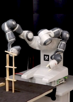
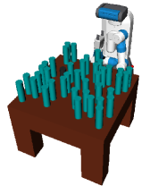
Recent years have witnessed immense progress in research on integrated task and motion planning [1, 2, 3, 4, 5, 6]. Research in this direction provides several approaches for solving deterministic, fully observable task and motion planning problems. However, the problem of integrated task and motion planning under uncertainty has been under-investigated. We consider integrated task and motion planning problems where the robot’s actions and its environment are stochastic. This problem is more difficult computationally because sequential plans are no longer sufficient; solutions take the form of policies that prescribe an action for every state that the robot may encounter during execution. For instance, consider the problem where a robot needs to pick up a can (black) from a cluttered table (Fig. 1). To achieve this objective, the robot needs to consider multiple contingencies, e.g., what if the can slips? What if it tumbles and rolls off when it is placed?

This example is representative of many real-world problems such as diffusing IEDs, operating live machinery, or assisting emergency response personnel. Safe robot execution in such situations requires pre-computation of truly feasible policies so as to reduce the need for time-consuming and error-prone on-the-fly replanning. A naïve approach for solving such problems would be to first compute a high-level policy using an abstract model of the problem (e.g., a model written in a language such as PPDDL or RDDL[7]), and to then refine each “branch” of the solution policy with motion plans. Such approaches fail because abstract models are lossy and policies computed using them might not have any feasible motion planning refinements [8, 9, 6]. Furthermore, as the planning horizon increases, computing complete task and motion policies becomes intractable as it requires the computation of exponentially many task and motion plans, one for each branch of the policy.

Figure 1: Left: YuMi robot uses the algorithm developed in this paper to build a $3\pi$ structure using Keva planks despite stochasticity in their initial locations. Right: A stochastic variant of the cluttered table domain where robot has to pick up the black can, but pickups may fail.

We present a novel anytime framework for computing integrated task and motion policies. Our approach continually improves the quality of solution policies while ensuring that the versions computed earlier can resolve situations that are more likely to be encountered during execution. It also provides a running estimate of the probability mass of likely executions covered in the current policy. This estimate can be used to start execution based on the level of risk acceptable in a given application, allowing one to trade-off precomputation time for on-the-fly invocation of our planner if an unhandled situation is encountered. Our approach generalizes methods for computing solutions for most-likely outcomes during execution [10, 11] to the problem of integrated task and motion planning by drawing upon approaches for anytime computation in AI planning [12, 13, 14]. Our experiments indicate the probability of encountering an unresolved contingency drops exponentially as the algorithm proceeds. The resulting approach is the first probabilistically complete algorithm for computing integrated task and motion policies in stochastic environments using a powerful relational representation for specifying input problems. Our approach uses arbitrary stochastic shortest path (SSP) planners and motion planners. This structure allows it to scale automatically with improvements in either of these active areas of planning research.

We begin with a presentation of the background definitions (II) and our formal framework (III). (IV) describes our overall algorithmic approach, followed by a description of empirical results using the Fetch and YuMi robot platforms (V), and a discussion of prior related work (VI).

II Background

A motion planning problem is a tuple $\langle C,f,p_{0},p_{t}\rangle$, where $C$ is the space of possible configurations or poses of a robot, $f(p)$ is a boolean function which determines whether the robot at config $p\in C$ is in collision with any object or not, and $p_{0},p_{t}\in C$ are the initial and final configs. A trajectory is a sequence of configurations. A collision-free motion plan for a motion planning problem is a trajectory in $C$ from $p_{0}$ to $p_{t}$ such that $f$ is false for any pose in the trajectory.

Stochastic shortest path (SSP) problems are a subclass of Markov decision processes (MDPs) that have absorbing states, the discounting factor $\gamma=1$ and a finite horizon [15]. An SSP can be defined as a tuple $\langle S,A,T,\mathcal{C},\gamma=1,H,s_{0},G\rangle$ where $S$ is a set of states; $A$ is a set of actions; $\forall s,s^{\prime}\in S,\quad a\in A\quad T(s,a,s^{\prime})=P(s^{\prime}|s,a)$; • $\mathcal{C}(s,a)$is the cost for action $a\in A$ in a state $s\in S$; • $H$is the length of the horizon; • $s_{0}$is an initial state; • $G$is the set of absorbing or goal states. A solution to an SSP is a policy $\pi$ of the form $\pi:S\times\{1,\dots,H\}\rightarrow A$ that maps all the states and time steps at which they are encountered to an action. The optimal policy $\pi^{*}$ is a policy that reaches the goal state with the least expected cumulative cost. SSP policies need not be stationary because the horizon is finite. Dynamic programming algorithms such as value iteration or policy iteration can be used to compute these policies. Value iteration for finite horizon SSPs can be defined as:

$$V^{0}(s) =0$$

$$V^{i}_{t}(s) =min_{a}\sum_{s^{\prime}}T(s,a,s^{\prime})\left[\mathcal{C}(s,a)+V^{i-1}_{t+1}(s^{\prime})\right]$$

$$\pi^{i}_{t}(s) =argmin_{a}\sum_{s^{\prime}}T(s,a,s^{\prime})\left[\mathcal{C}(s,a)+V^{i-1}_{t+1}(s^{\prime})\right]$$

III Formal Framework

We model stochastic task and motion planning problems as abstracted SSPs where each action of the SSP (e.g. place) corresponds to an infinite set of motion planning problems. The overall problem is to compute a policy for the SSP along with “refinements” that select, for each action in the policy, a specific motion planning problem and its solution. E.g., the “high-level” action for placing a can on a table corresponds to infinitely many motion planning problems, each defined by a target pose for the can. The refinement process would thus need to select the pose that the gripper should be in prior to opening, and a motion plan for each occurrence of the pickup action in the computed policy.

Formalization of abstraction functions    To formalize the necessary abstractions we first introduce some notation. We denote states as logical models or structures. We use the term logical structures or structures to distinguish the concept from SDM models. A structure $S$, of vocabulary $\mathcal{V}$, consists of a universe $\mathcal{U}$, along with a relation $r^{S}$ over $\mathcal{U}$ for every relation symbol $r$ in $\mathcal{V}$ and an element $c^{S}\in\mathcal{U}$ for every constant symbol $c$ in $\mathcal{V}$. We denote the value of a term or formula $\varphi$ in a structure $S$ as $\llbracket\varphi\rrbracket_{S}$.We also extend this notation so that $\llbracket r\rrbracket_{S}$ denotes the interpretation of the relation $r$ in $S$. We consider relations as a special case of functions.

We formalize abstractions using first-order queries [16, 17] that map structures over one vocabulary to structures over another vocabulary. In general, a first-order query $\alpha$ from $V_{\ell}$ to $V_{h}$ defines functions in $\alpha(S_{\ell})$ using interpretations of $V_{\ell}$-formulas in $S_{\ell}$: $\llbracket r\rrbracket_{\alpha(S_{\ell})}(o_{1},\ldots o_{n})=True$ iff $\llbracket\varphi^{\alpha}_{r}(o_{1},\ldots o_{n})\rrbracket_{S_{\ell}}=\emph{True}$, where $\varphi^{\alpha}_{r}$ is a formula over $V_{\ell}$.

We define relational abstractions as first-order queries where $V_{h}\subset V_{\ell}$; the predicates in $V_{h}$ are defined as identical to their counterparts in $V_{\ell}$. Such abstractions reduce the number of properties being modeled. Let $\mathcal{U_{\ell}}$ ($\mathcal{U}_{h}$) be the universe of $S_{\ell}$ ($S_{h}$) such that $|\mathcal{U}_{h}|\leq|\mathcal{U}_{\ell}|$. Function abstractions do not reduce the number of objects being considered.

Let $\rho:\mathcal{U}_{h}\rightarrow 2^{\mathcal{U}_{\ell}}$ be a collection function that maps elements in $\mathcal{U}_{h}$ to the collection of $\mathcal{U}_{\ell}$ elements that they represent. E.g., $\rho(\emph{Kitchen})=\{\emph{loc}:\land_{i}~{}\emph{loc}\cdot\emph{BoundaryVector}_{i}<0\}$ where the kitchen has a polygonal boundary.

We define an entity abstraction $\alpha_{\rho}$ using the collection function $\rho$ as $\llbracket r\rrbracket_{\alpha_{\rho}(S_{\ell})}(\tilde{o}_{1},\ldots\tilde{o}_{n})=True$ iff $\exists o_{1},\ldots o_{n}$ such that $o_{i}\in\rho(\tilde{o}_{i})$ and $\llbracket\varphi^{\alpha_{\rho}}_{r}(o_{1},\ldots o_{n})\rrbracket_{S_{\ell}}=\emph{True}$. We omit the subscript $\rho$ when it is clear from context. Entity abstractions define the truth values of predicates over abstracted entities as the disjunction of the corresponding concrete predicate instantiations (an object is in the abstract region “kitchen” if it is at any location in that region). Such abstractions have been used for efficient generalized planning [18] as well as answer set programming [19].

STAMP Problems    We define STAMP problems using abstractions as follows.

Definition 1

A stochastic task and motion planning problem (STAMPP) $\langle{\cal M},c_{0},\alpha,[{\cal M}]\rangle$ is defined using a concrete SSP ${\cal M}$, its abstraction $[{\cal M}]$ obtained using a composition of function and entity abstractions, denoted as $\alpha$, and the initial concrete configuration of the environment $c_{0}$.

Solutions to STAMPPs, like solutions to an SSP, are policies with actions from the concrete model ${\cal M}$.

Let $S$ be the set of abstract states generated when an abstraction function $\alpha$ is applied on a set of concrete states $X$. For any $s\in S$, the concretization function $\Gamma_{\alpha}(s)=\{x\in X:\alpha(x)=s\}$ denotes the set of concrete states represented by the abstract state $s$. For a set $C\subseteq X$, $[C]_{\alpha}$ denotes the smallest set of abstract states representing $C$. Generating the complete concretization of an abstract state can be computationally intractable, especially in cases where the concrete state space is continuous. In such situations, the concretization operation can be implemented as a generator that incrementally samples elements from an abstract argument’s concrete domain.

Place($obj_{1}$, $config_{1}$, $config_{2}$, $target\_pose$, $traj_{1}$)
precon RobotAt($config_{1}$), holding($obj_{1}$), IsValidMP($traj_{1}$, $config_{1}$, $config_{2}$), IsPlacementConfig($obj_{1}$, $config_{2}$,           $target\_pose$) concrete effect $\lnot$holding($obj_{1}$), $\forall traj$ intersects(vol(obj ,target_pose), sweptVol(robot, traj)$\rightarrow$ Collision($obj_{1}$, traj), probabilistic:    0.8 [RobotAt($config_{2}$),      at($obj_{1}$, $target\_pose$)]    0.2 [RobotAt($around\_config_{2}$),      at($obj_{1}$,$around\_target\_pose$)] abstract effect $\lnot$holding($obj_{1}$), $\forall traj$ \raisebox{-.9pt} {{\small?}}⃝ Collision($obj_{1}$, $traj$), probabilistic:    0.8 [RobotAt($config_{2}$),      at($obj_{1}$, $target\_pose$)]    0.2 [RobotAt($around\_config_{2}$),      at($obj_{1}$,$around\_target\_pose$)]

Figure 2: Concrete (above) and abstract (below) effects of a one-handed robot’s action for placing an object.

Example    Consider the specification of a robot’s action of placing an item as a part of an SSP. In practice, low-level accurate models of such actions may be expressed as generative models, or simulators. Fig. 2 helps identify the nature of abstract representations needed for expressing such actions. For readability, we use a convention where preconditions are comma-separated conjunctive lists and universal quantifiers represent conjunctions over the quantified variables. Numbers represent the probability of that outcome.

The concrete, unabstracted, description of this action (Fig. 2) requires action arguments representing the object to be placed ($\emph{obj}_{1}$), the initial and final robot configurations ($\emph{config}_{1}$, $\emph{config}_{2}$), the target pose for the object ($\emph{target}\_\emph{pose}$), and the motion planning trajectory ($\emph{traj}_{1}$) to be used. These arguments represent the choices to be made when placing an object. The preconditions of Place express the conditions that the robot is in $\emph{config}_{1}$; it is holding the object $\emph{obj}_{1}$; $\emph{traj}_{1}$ is a motion plan which moves robot from $\emph{config}_{1}$ to $\emph{config}_{2}$ (IsValidMP); $\emph{config}_{2}$ corresponds to the object being at the target pose in the gripper (IsPlacementConfig). We ignore the gripper open configuration for ease in exposition.

This action model specifies two probabilistic effects. The robot moves to $config_{2}$ and places the object successfully at $\emph{target}\_\emph{pose}$ with probability 0.8. It moves to some other configuration $\emph{around}\_\emph{config}_{2}$ and places the object at a location $\emph{around}\_\emph{target}\_\emph{pose}$ with probability 0.2. In both cases, the robot is no longer holding the object and it collides with objects that lie in the volume swept by the robot while following the trajectory. The intersects predicate is static as it operates on volumes, while Collision changes with the state.

We use entity abstraction to replace each continuous action argument with a symbol denoting a region that satisfies the precondition subformulas where that argument occurs. This may require Skolemization as developed in prior work [6]. Effects of abstract actions on symbolic arguments cannot be determined precisely; their values are assigned by the planning algorithm. E.g., it is not possible to determine in the abstract model whether the placement trajectory will be in collision. Such predicates are annotated in the set of effects with the symbol \raisebox{-.9pt} {{\small?}}⃝ (see the abstract effect in Fig. 2). This results in a sound abstract model [6, 20].

IV Algorithmic Framework

IV-A Overall Approach

We now describe our approach for computing task and motion policies as defined above. For clarity, we begin by describing certain choices in the algorithm as non-deterministic. Variants of our overall approach can be constructed with different implementations of these choices; the versions used in our evaluation are described in IV-B.

Recall that abstract grounded actions $[a]\in[{\cal M}]$ (e.g., Place(cup, config1_cup, config2_cup, target_pose_cup, traj1_cup)) have symbolic arguments that can be instantiated to yield concrete grounded actions $a\in{\cal M}$.

Our overall algorithm interleaves computation among the processes of (a) concretizing an abstract policy, (b) updating the abstraction to include predicate valuations for a fixed concretization, and (c) computing an abstract policy for an updated abstract state. This is done using the plan refinement graph (PRG). Every node u in the PRG represents an abstract model $[{\cal M}]_{u}$, an abstract policy $[\pi]_{u}$ in the form of a tree whose vertices represent states and edges represent action applications, the current state of the search for concretizations of all actions $a_{j}$ $\in$ $[\pi]_{u}$, and a partial concretization $\sigma_{u}$ for a topological prefix of the policy tree $[\pi]_{u}$. Each edge (u,v) between nodes u and v in the PRG is labeled with a partial concretization $\sigma_{u,v}$ and the failed preconditions for the first abstract action in a root-to-leaf path in $[\pi]_{u}$ which doesn’t have a feasible refinement under $\sigma_{u,v}$. Recall that this occurs because the abstract model is lossy and doesn’t capture precise action semantics. $[{\cal M}]_{v}$ is the version of $[{\cal M}]_{u}$ where the predicates corresponding to the failed preconditions (corresponding to effects with \raisebox{-.9pt} {{\small?}}⃝, created due to the abstraction discussed in Sec. III) have been replaced with their literal versions that are true under $\sigma_{u,v}$.

ATM-MDP algorithm (Alg.1) carries out the interleaved search outlined above as follows. It first initializes the PRG with a single node containing an abstract policy for the abstract SSP (line 1). In every iteration of the main loop, it selects a node in the PRG and extracts an unrefined root-to-leaf path from the policy for that node (lines 3-5). It then interleaves the three processes as follows.

a) Concretization of an available policy

Lines 7-13 search for a feasible concretization (refinement) of the partial path by instantiating its symbolic action arguments with values from their original non-symbolic domains. Trajectory symbols like $traj_{1}$ are refined using motion planners. A concretization $c_{0},a_{1},c_{1},\ldots,a_{k},c_{k}$ of the path $[s_{0}],[a_{1}],[s_{1}],\ldots,[a_{k}],[s_{k}]$ is feasible starting with a concrete initial state $c_{0}$ iff $c_{i+1}\in a_{i+1}(c_{i})$ and $c_{i}\models PRECOND(a_{i+1})$ for $i=0,\ldots,k-1$. However, it is possible that $[\pi]$ admits no feasible concretization because every instantiation of the symbolic arguments violates the preconditions of some action in $\{\pi_{i}\}$. For example, an infeasible path would have the robot placing a cup on the table in the concrete state $c_{0}$, when every possible motion plan for doing so may be in collision with some object(s).

b) Update abstraction for a fixed concretization

Lines 16-20 fix a concretization for the partially refined path selected on line 6, and identify the earliest abstract state in this path whose subsequent action’s concretization is infeasible. This abstract state is updated with the true forms of the violated preconditions that hold in this concretization, using symbolic arguments. E.g., Collision($teapot$, $traj\_cup$). The rest of the policy after this abstract state is discarded. A state update is immediately followed by the computation of a new abstract policy (see below).

c) Computation of a new abstract policy

Lines 21-22 compute a new policy with the updated information computed under (b). The SSP solver is invoked to compute a new policy from the updated state; its solution policy is unrolled as a tree of bounded depth and appended to the partially refined path. This allows the time horizon of the policy to be increased dynamically.

Several optimizations can be made while selecting a PRG node to concretize or update in line 3. We used iterative-broadening depth-first search on the PRG with the max breadth incremented by $5$ in each iteration.

In our implementation the Compute variable on line 6 is set to either Concretization or UpdateAbstraction with probability $0.5$. The explore parameter on line 9 needs to be set with non-zero probability for a formal guarantee of completeness, although in our experiments it was set to False.

Input: model $[{\cal M}]$, domain $\mathcal{D}$, problem $\mathcal{P}$, SSP Solver SSP, Motion Planner $M$

Output: anytime, contingent task and motion policy

1 Initialize PRG with a node with an abstract policy $[\pi]$ for $P$ computed by SSP;

2 while solution of desired quality not found do

3       PRNode $\leftarrow$ GetPRNode();

4       $[\pi]$ $\leftarrow$ GetAbstractPolicy($[{\cal M}]$, PRNode, $\mathcal{D}$, $\mathcal{P}$, SSP);

5       path_to_refine $\leftarrow$ GetUnRefinedPath($[\pi]$);

6       Compute $\leftarrow$ NDChoice{Concretization, UpdateAbstraction};

7       if Compute = Concretization then

8             while $[\pi]$ has an unrefined path and resource limit is not reached do

                   if explore// non-deterministic

9                   then

10                         replace a suffix of partial_path with a random action;

11                        

12                   end if

13                  search for a feasible concretization of path_to_refine;

14                  

15             end while

16            

17       end if

18      if Compute = UpdateAbstraction then

19             partial_path $\leftarrow$ GetUnrefinedSuffix(PRNode, path_to_refine);

20             $\sigma\leftarrow$ ConcretizeLastUnrefinedAction($[\pi]$);

21             failure_reason $\leftarrow$ GetFailedPrecondition($[\pi]$, $\sigma$ );

22             updated_state $\leftarrow$ UpdateState($[\pi]$, failure_reason);

23             $[\pi^{\prime}]\leftarrow$ merge($[\pi]$, solve(updated_state, $G$, $[{\cal M}]$));

24             generate_new_pr_node($[\pi^{\prime}]$, $[{\cal M}]$);

25            

26       end if

27      

28 end while

Algorithm 1 ATM-MDP Algorithm

IV-B Optimizations and Formal Results

We develop the basic algorithm outlined above (Alg. 1) along two major directions: we enhance it to facilitate anytime computation and to improve the search for concretizations of abstract policies.

Anytime computation for task and motion policies

The main computational challenge for the algorithm is that the number of root-to-leaf (RTL) branches grows exponentially with the time horizon and the contingencies in the domain. Each RTL branch has a certain probability of being encountered; refining it incurs a computational cost. Waiting for a complete refinement of the policy tree results in wasting a lot of time as most of the situations have a very low probability of being encountered. The optimal selection of the paths to refine within a fixed computational budget can be reduced to the knapsack problem. Unfortunately, we do not know the precise computational costs required to refine a path. However, we can approximate this cost depending on the number of actions and the size of the domain of the arguments in those actions. Furthermore, the knapsack problem is NP-hard. However, we can compute provably good approximate solutions to this problem using a greedy approach: we prioritize the selection of a path to refine based on the probability of encountering that path p and the estimated cost of refining that path c. We compute $p/c$ ratio for all the paths and select the unrefined path with largest ratio for refinement.

Figure 3: Left: Backtracking from node B invalidates the refinement of subtree rooted at A. Right: Replanning from node B.

Search for concretizations

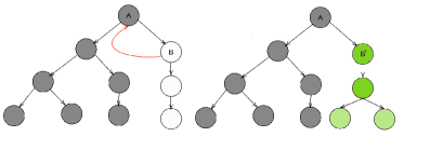
Sample-based backtracking search for concretization of symbolic variables [6] suffers from a few limitations in stochastic settings that are not present in deterministic settings. Fig. 3 illustrates the problem. In this figure, grey nodes represent actions in the policy tree that have already been refined; the refinement for B is being computed. White nodes represent the nodes that still require refinement. If backtracking search changes the concretization for B’s parent (Fig. 3, left) it will invalidate the refinements made for the entire subtree rooted at that node. Instead, it may be better to compute an entirely new policy for B (effectively jumping to the UpdateAbstraction mode of computation on line 16 from line 13).

Thm. 1 formalizes the anytime performance of ATM-MDP and Thm. 2 shows that our solution to this problem is probabilistically complete. Additional details about these results are available in the extended version of the paper [21].

Theorem 1

Let $t$ be the time since the start of the algorithm at which the refinement of any $RTL$ path is completed. If path costs are accurate and constant then the total probability of unrefined paths at time $t$ is at most $1-opt(t)/2$, where $opt(t)$ is the best possible refinement (in terms of the probability of outcomes covered) that could have been achieved in time $t$.

Proof:

(Sketch) Let $c$ be the cost of refining some RTL path and $\hat{c}$ be an approximation of it. The proof follows from the fact that the greedy algorithm achieves a 2-approximation for the knapsack problem and that for all RTL paths, $\hat{c}\geq c$. So the priority queue will never underestimate the relative costs, and algorithm’s coverage of high-probability contingencies will be no further from the optimal than the bound suggested in the theorem. ∎

Theorem 2

If there exists a proper policy that reaches the goal within horizon h with probability p, and has feasible low-level refinement, then Alg. 1 will find it with probability $1.0$ in the limit of infinite samples.

Proof:

(Sketch) Let $\pi_{p}$ be a proper policy. For some policy $\pi$ in PRG, let $k$ denote the minimum depth up to which $\pi_{p}$ and $\pi$ match. If there are no feasible refinements possible for an action at depth $k+1$ in $\pi$, then the explore step (line 11) would replace that action such that it matches the action at depth $k+1$ in $\pi_{p}$ with some non-zero probability (given that actions are finite). Once the algorithm finds policy $\pi$ which matches $\pi_{p}$, the backtracking search will find a feasible refinement if the measure of these refinements under the probability density of generators is non-zero. ∎

V Empirical Evaluation

We implemented the presented framework using an open-source implementation from MDP-Lib github repository  [22] of LAO* [23] as the SSP solver, the OpenRAVE [24] robot simulation system along with its collision checkers, CBiRRT implementation from PrPy suite  [25] for motion planning. Since there are no common benchmarks for evaluating stochastic task and motion planning problems, we evaluated our algorithm on 7 diverse and challenging test problems over 4 domains and evaluated 5 of those problems with physical robot systems. In practice, fixing the horizon $h$ a priori can render some problems unsolvable. Instead, we implemented a variant that dynamically increases the horizon until the goal is reached with probability greater than $0$. We evaluated our approach on a variety of problems where combined task and motion planning is necessary. The source code and the videos for our experiments experiment can be found at https://aair-lab.github.io/stamp.html.

Problem	% Solved	Avg. Time (s)
Cluttered-15	95	1093.71
Cluttered-20	79	1144.85
Cluttered-25	74	1392.83
Aircraft Inspection	100	1457.08
$3\pi$	100	1312.83
Tower-12	100	1899.73
Twisted-Tower-12	98	1984.29
Domino $(n=10,k=2)$	100	98.64
Domino $(n=10,k=3)$	100	350.63
Domino $(n=15,k=2)$	100	179.60
Domino $(n=15,k=3)$	100	631.91
Domino $(n=20,k=2)$	100	350.60
Domino $(n=20,k=3)$	100	590.60

Figure 4: Summary of times taken to solve the test problems. Timeout for cluttered table, aircraft inspection, and Domino: 2400 seconds, building Keva stuctures: 4000 seconds.

(a) The Fetch mobile manipulator uses a STAMP policy to pickup a target bottle while avoiding those that are likely to be crushed. It replaces a bottle that wasn’t crushed (left), discards a bottle that was crushed (center) and picks up the target bottle (right).

(b) ABB YuMi builds Keva structures using a STAMP policy: 12-level tower (left), twisted 12-level tower (center), and $3$-towers (right).

Figure 5: Photos from our evaluation using the Fetch and YuMi robots. Videos are available at https://aair-lab.github.io/stamp.html.

Figure 6: Anytime performance of ATM-MDP, showing the time in seconds (x-axis) vs. probability mass refined (y-axis).

Cluttered Table

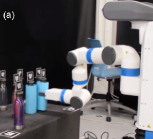
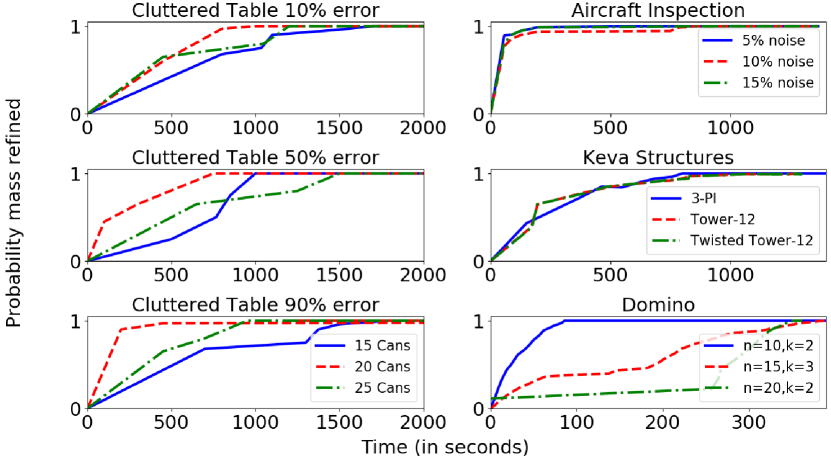
In this problem, we have a table cluttered with cans having different probabilities of being crushed when grabbed by the robot. Some cans are delicate and are highly likely to be crushed when the robot grabs them, incurring a high cost (probability for crushing was set to 0.1, 0.5 & 0.9 in different experiments in Fig. 6(a)), while others are normal and are less likely to be crushed (with probability set to 0.05). The goal of the robot is to pick up a specific can. We used different numbers of cans (15, 20, 25), and different random configurations of cans to extensively evaluate the proposed framework. We also used this scenario to evaluate our approach in the real-world (Fig. 5(a)) using the Fetch mobile manipulation robot [26].

Aircraft Inspection

In this problem, an unmanned aerial vehicle (UAV) needs to inspect possibly faulty parts of an aircraft. Its goal is to locate the fault and notify the supervisor about it. However, its sensors are not accurate and may fail to locate the fault with some non-zero probability (failure probability was set to 0.05, 0.1, & 0.15 for experiments in Fig. 6(b)) while inspecting the location; it may also drift to another location while flying. Charging stations are available for the UAV to dock and charge itself. All movements use some amount of battery charge depending on the length of the trajectory, but the high-level planner cannot determine whether the current level of the battery is sufficient for an action as it doesn’t have access to precise trajectories. This makes it necessary for the high-level to obtain feedback from the low-level to solve the problem.

Domino

In this problem, the YuMi robot [27] needs to pick up a domino from a table that has $n$ dominos on it. It has to notify the human about toppled dominos. While trying to pick up a domino, $k$ domino’s on each side can topple adding up to $2^{2k}$ contingencies that might need refinement.

Building structures using Keva planks

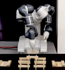
In this problem, the YuMi robot [27] needs to build different structures using Keva planks. Keva planks are laser cut wooden planks with uniform geometry. Fig. 5(b) and Fig. 1 show some of the target structures. Planks are placed one at a time by a user after each pickup and placement by the YuMi. Each new plank may be placed at one of a few predefined locations, which adds uncertainty in the planks’ initial location. For our experiments, two predefined locations were used to place the planks with a probability of 0.8 for the first location and a probability of 0.2 for the second location. In this problem, hand-written goal conditions are used to specify the desired target structure. The YuMi [27] needs to create a task and motion policy for successively picking up and placing planks to build the structure. There are infinitely many configurations in which one plank can be placed on another, but the abstract model blurs out different regions on the plank. The put-down pose generator uses the target structure to concretize each plank’s target put-down pose. State-of-the-art SSP solvers fail to compute abstract solution policies for structures of height greater than 3 for this problem. However, these structure-building problems exhibit repeating substructure every 1-2 layers that reuse minor variants of the same abstract policy. We used this observation to develop an SSP solver that incrementally calls LAO* to compute iterative policies. The results for Keva structures use this solver. In addition to the test problems shown in Fig. 4 this allows our approach to scale to more complex problems such as 3-towers (Fig. 5). Approaches for generalized planning [28, 29, 30, 18] could be used to automatically extract and utilize such patterns in other problems with repeating structures.

V-A Analysis of Results

Fig. 6 shows the anytime characteristics of our approach in all of the test domains. The y-axis shows the probability with which the policy available at any time during the algorithm’s computation will be able to handle all possible execution-time outcomes, and the x-axis shows the time (seconds) required to refine that probability mass.

These results indicate that in all of our test domains, the refined probability mass increases rapidly with time so that about 80% of probable executions are covered within about 30% of the computation time. Fig. 6 also shows that refining the entire policy tree requires a significant time. This reinforces the need for an anytime solution in such problems.

Fig. 4 shows average times taken to compute complete STAMP policies for our test problems. These values are averages of 50 runs for cluttered table, 20 runs for aircraft inspection and 15 runs for Keva structures. Aircraft inspection problems and Keva structure problems required fewer runs because their runtimes showed negligible variance.

VI Other Related Work

There has been a renewed interest in integrated task and motion planning algorithms. Most research in this direction has been focused on deterministic environments [8, 31, 32, 9, 33, 34, 35]. Kaelbling and Lozano-Perez [36] consider a partially observable formulation of the problem. Their approach utilizes regression modules on belief fluents to develop a regression-based solution algorithm. While they address the more general class of partially observable problems, their approach follows a process of online, incremental discretization and does not address the computation of branching policies, which is the focus of this paper. Sucan and Kavraki [37] use an explicit multigraph to represent the problem for which motion planning refinements are desired. Other approaches [10] address problems where the high-level formulation is deterministic and the low-level is determinized using most likely observations. Our approach uses a compact, relational representation; it employs abstraction to bridge SSP solvers and motion planners and solves the overall problem in anytime fashion. Preliminary versions of this work [38, 39] were presented at non-archival venues and did not include the full formalization and optimizations required to solve the realistic tasks prsented in this paper.

Several approaches utilize abstraction for solving MDPs [40, 41, 42, 43]. However, these approaches assume that the full, unabstracted MDP can be efficiently expressed as a discrete MDP. Marecki et al. [44] consider continuous-time MDPs with finite sets of states and actions. In contrast, our focus is on MDPs with high-dimensional, uncountable state and action spaces. Recent work on deep reinforcement learning (e.g., [45, 46]) presents approaches for using deep neural networks in conjunction with reinforcement learning to solve short-horizon MDPs with continuous state spaces. These approaches can be used as primitives in a complementary fashion with task and motion planning algorithms, as illustrated in recent promising work by Wang et al. [47].

References

- [1] C. R. Garrett, T. Lozano-Pérez, and L. P. Kaelbling, “Ffrob: Leveraging symbolic planning for efficient task and motion planning,” IJRR, vol. 37, no. 1, pp. 104–136, 2018. [Online]. Available: https://doi.org/10.1177/0278364917739114
- [2] N. T. Dantam, Z. K. Kingston, S. Chaudhuri, and L. E. Kavraki, “An incremental constraint-based framework for task and motion planning,” IJRR, vol. 37, no. 10, pp. 1134–1151, 2018.
- [3] M. Cashmore, M. Fox, D. Long, D. Magazzeni, B. Ridder, A. Carrera, N. Palomeras, N. Hurtos, and M. Carreras, “Rosplan: Planning in the robot operating system,” in In Proc. ICAPS, 2015.
- [4] C. R. Garrett, T. Lozano-Pérez, and L. P. Kaelbling, “Stripstream: Integrating symbolic planners and blackbox samplers,” Computing Research Repository, vol. abs/1802.08705, 2018. [Online]. Available: http://arxiv.org/abs/1802.08705
- [5] R. Chitnis, D. Hadfield-Menell, A. Gupta, S. Srivastava, E. Groschev, C. Lin, and P. Abbeel, “Guided search for task and motion plans using learned heuristics,” in In Proc. ICRA, 2016.
- [6] S. Srivastava, E. Fang, L. Riano, R. Chitnis, S. Russell, and P. Abbeel, “A modular approach to task and motion planning with an extensible planner-independent interface layer,” in In Proc. ICRA, 2014.
- [7] S. Sanner, “Relational dynamic influence diagram language (rddl): Language description,” 2010, http://users.cecs.anu.edu.au/~ssanner/IPPC˙2011/RDDL.pdf.
- [8] S. Cambon, R. Alami, and F. Gravot, “A hybrid approach to intricate motion, manipulation and task planning,” IJRR, vol. 28, pp. 104–126, 2009.
- [9] L. P. Kaelbling and T. Lozano-Pérez, “Hierarchical task and motion planning in the now,” in In Proc. ICRA, 2011.
- [10] D. Hadfield-Menell, E. Groshev, R. Chitnis, and P. Abbeel, “Modular task and motion planning in belief space,” in In Proc. IROS, 2015.
- [11] S. Yoon, A. Fern, and R. Givan, “FF-replan: A baseline for probabilistic planning,” in In Proc. ICAPS, 2007.
- [12] T. L. Dean and M. S. Boddy, “An analysis of time-dependent planning.” in In Proc. AAAI, 1988.
- [13] S. Zilberstein and S. J. Russell, “Anytime sensing, planning and action: A practical model for robot control,” in Proc. IJCAI, 1993.
- [14] T. Dean, L. P. Kaelbling, J. Kirman, and A. Nicholson, “Planning under time constraints in stochastic domains,” Artificial Intelligence, vol. 76, no. 1-2, pp. 35–74, 1995.
- [15] D. P. Bertsekas and J. N. Tsitsiklis, “An analysis of stochastic shortest path problems,” Mathematics of Operations Research, vol. 16, no. 3, pp. 580–595, 1991.
- [16] E. F. Codd, “Relational completeness of data base sublanguages,” in Database Systems, R. R, Ed., 1972.
- [17] N. Immerman, Descriptive complexity. Springer Science & Business Media, 1998.
- [18] S. Srivastava, N. Immerman, and S. Zilberstein, “A new representation and associated algorithms for generalized planning,” Artificial Intelligence, vol. 175, no. 2, pp. 615–647, 2011.
- [19] Z. G. Saribatur, P. Schüller, and T. Eiter, “Abstraction for non-ground answer set programs,” in In Proc.JELIA, 2019.
- [20] S. Srivastava, S. Russell, and A. Pinto, “Metaphysics of planning domain descriptions,” in In Proc. AAAI, 2016.
- [21] N. Shah, K. Kumar, P. Khamojhalla, D. Kala Vasudevan, and S. Srivastava, “Anytime integrated task and motion policies for stochastic environments,” Arizona State University, School of Computing, Informatics, and Decision System Engineering, Tech. Rep. ASUCISE-2019-001, 2019. [Online]. Available: https://aair-lab.github.io/stamp.html
- [22] L. Pineda, “MDP-Lib,” https://github.com/luisenp/mdp-lib, 2014.
- [23] E. A. Hansen and S. Zilberstein, “LAO∗: A heuristic search algorithm that finds solutions with loops,” Artificial Intelligence, vol. 129, no. 1-2, pp. 35–62, 2001.
- [24] R. Diankov, “Automated construction of robotic manipulation programs,” Ph.D. dissertation, Carnegie Mellon University, 2010.
- [25] M. Koval, “Prpy,” https://github.com/personalrobotics/prpy, 2015.
- [26] M. Wise, M. Ferguson, D. King, E. Diehr, and D. Dymesich, “Fetch and freight: Standard platforms for service robot applications,” in Workshop on Autonomous Mobile Service Robots, 2016.
- [27] A. Robotics, “Abb yumi,” URL: http://new.abb.com/products/robotics/yumi/, vol. 9, 2015.
- [28] S. Srivastava, N. Immerman, and S. Zilberstein, “Learning generalized plans using abstract counting,” in In Proc. AAAI, 2008.
- [29] B. Bonet, H. Palacios, and H. Geffner, “Automatic derivation of memoryless policies and finite-state controllers using classical planners,” in In Proc. ICAPS, 2009.
- [30] Y. Hu and G. De Giacomo, “Generalized planning: Synthesizing plans that work for multiple environments,” in In Proc. IJCAI, 2011.
- [31] E. Plaku and G. D. Hager, “Sampling-based motion and symbolic action planning with geometric and differential constraints,” in In Proc. ICRA, 2010.
- [32] A. Hertle, C. Dornhege, T. Keller, and B. Nebel, “Planning with semantic attachments: An object-oriented view,” in In Proc. ECAI, 2012.
- [33] C. R. Garrett, T. Lozano-Pérez, and L. P. Kaelbling, “FFrob: An efficient heuristic for task and motion planning,” in In Proc. WAFR, 2015.
- [34] N. T. Dantam, Z. K. Kingston, S. Chaudhuri, and L. E. Kavraki, “Incremental task and motion planning: A constraint-based approach.” in In Proc. RSS, 2016.
- [35] C. R. Garrett, T. Lozano-Pérez, and L. P. Kaelbling, “Sampling-based methods for factored task and motion planning,” IJRR, vol. 37, no. 13-14, pp. 1796–1825, 2018.
- [36] L. P. Kaelbling and T. Lozano-Pérez, “Integrated task and motion planning in belief space,” IJRR, vol. 32, no. 9-10, pp. 1194–1227, 2013.
- [37] I. A. Şucan and L. E. Kavraki, “Accounting for uncertainty in simultaneous task and motion planning using task motion multigraphs,” in In Proc. ICRA, 2012.
- [38] S. Srivastava, N. Desai, R. Freedman, and S. Zilberstein, “An anytime algorithm for task and motion mdps,” arXiv preprint arXiv:1802.05835, 2018.
- [39] N. Shah and S. Srivastava, “Anytime integrated task and motion policies for stochastic environments,” ArXiv, vol. abs/1904.13006, 2019.
- [40] J. Hostetler, A. Fern, and T. Dietterich, “State aggregation in monte carlo tree search.” in In Proc. AAAI, 2014.
- [41] A. Bai, S. Srivastava, and S. J. Russell, “Markovian state and action abstractions for MDPs via hierarchical MCTS.” in In Proc. IJCAI, 2016.
- [42] L. Li, T. J. Walsh, and M. L. Littman, “Towards a unified theory of state abstraction for mdps.” in In Proc. ISAIM, 2006.
- [43] S. P. Singh, T. Jaakkola, and M. I. Jordan, “Reinforcement learning with soft state aggregation,” in In Proc. NIPS, 1995.
- [44] J. Marecki, Z. Topol, M. Tambe, et al., “A fast analytical algorithm for mdps with continuous state spaces,” in In Proc. AAMAS, 2006.
- [45] M. Hausknecht and P. Stone, “Deep reinforcement learning in parameterized action space,” in In Proc. ICLR, 2016.
- [46] V. Mnih, K. Kavukcuoglu, D. Silver, A. A. Rusu, J. Veness, M. G. Bellemare, A. Graves, M. Riedmiller, A. K. Fidjeland, G. Ostrovski, et al., “Human-level control through deep reinforcement learning,” Nature, vol. 518, no. 7540, pp. 529–533, 2015.
- [47] Z. Wang, C. R. Garrett, L. P. Kaelbling, and T. Lozano-Pérez, “Active model learning and diverse action sampling for task and motion planning,” in In Proc. IROS, 2018.