Triangle Preferential Attachment Has Power-law Degrees and Eigenvalues; Eigenvalues Are More Stable to Network Sampling
Preferential attachment models are a common class of graph models which have been used to explain why power-law distributions appear in the degree sequences of real network data. One of the things they lack, however, is higher-order network clustering, including non-trivial clustering coefficients. In this paper we present a specific Triangle Generalized Preferential Attachment Model (TGPA) that, by construction, has nontrivial clustering. We further prove that this model has a power-law in both the degree distribution and eigenvalue spectra. We use this model to investigate a recent finding that power-laws are more reliably observed in the eigenvalue spectra of real-world networks than in their degree distribution. One conjectured explanation for this is that the spectra of the graph is more robust to various sampling strategies that would have been employed to collect the real-world data compared with the degree distribution. Consequently, we generate random TGPA models that provably have a power-law in both, and sample subgraphs via forest fire, depth-first, and random edge models. We find that the samples show a power-law in the spectra even when only 30% of the network is seen. Whereas there is a large chance that the degrees will not show a power-law. Our TGPA model shows this behavior much more clearly than a standard preferential attachment model. This provides one possible explanation for why power-laws may be seen frequently in the spectra of real world data.
1 Introduction
The idea of preferential attachment (PA) has a lengthy history in explaining “rich-get-richer” models Yule [1925]; Price [1976]. In the context of networks, a preferential attachment model suggests that when agents join a network, they form links to existing nodes with large degrees. These models offer a simple local rule that helps explain the presence of highly-skewed or power-law degree distributions in real-world networks Barabási and Albert [1999]. While a simple and compelling mathematical model, there are weaknesses in the relationship between PA models and real-world data. One of the most striking is the lack of clustering in PA network models. Consequently, there has been a line of work on generalized PA models that include ways to address the lack of clustering. First, Holme and Kim [2002] proposed a triangle PA model, where agents arrive and link to a node based on its degree and also link to a neighbor of that node to form a triangle. Later, Ostroumova et al. [2013] generalized a family of PA models and showed that they had power-law degree distributions and high-clustering.
Our work follows in this vein, although we adapt a slightly different notion of a triangle PA model that builds on a recent proposal to show how preferential attachment could give a power-law with any exponent Avin et al. [2017]. The specific Triangle Generalized Preferential Attachment model we use has two slightly different forms as explained in Section 4. The two forms are used to greatly simplify the analysis of the resulting properties. We do not believe there to be qualitative differences between them. Formally, we show that these models have a power-law in the degree distribution (Theorem 7, Corollary 14) as well as a power-law in the eigenvalues of the adjacency matrix (Theorem 8).
We also find empirically that our TGPA model has higher-order clustering in terms of higher-order clique closures Yin et al. [2018] that is characteristic of real-world data (Section 7).
Our interest in the TGPA model stems from our recent finding on the reliable presence of power-laws in the eigenvalue spectrum of the adjacency matrix Eikmeier and Gleich [2017]. Specifically, Eikmeier and Gleich [2017] found that real-world networks of a variety of types were more likely to have a statistically significant power-law in the eigenvalues of the adjacency matrix than in the degree distribution. This observation presents a simple question, might this behavior be expected in light of how real-world network data are collected? To be specific, real-world network data reflect two types of sampling artifacts. They are often built from a process run on a larger dataset. Consider how web and social networks are often crawled by programs that use breadth-first or related crawling strategies. Second, the crawled data itself represents a sample of some underlying (and unknown) latent network Schoenebeck [2013]. Again, note that the social links on networks such as Facebook and Twitter only represent a sample of some unobserved true social network. Because of the way that individuals join these networks, forest-fire models are often used to simulate this type of artifact.
Consequently, we study how often samples of TGPA models have statistically significant power laws in their degrees and eigenvalues (Section 8). These results (Figure 8) offer compelling evidence that the eigenvalues of the adjacency matrix robustly indicate the presence of a power-law, with more reliability than the degrees. It should be noted that the presence (or lack thereof) of power-laws in real world data has been often debated Meusel et al. [2015]; Gjoka et al. [2010]; Broido and Clauset [2019]. For that reason, we study models where they are unambiguously present. Although other PA models have the needed property of power-laws in both spectra and degrees, we find that the differences in behavior between the sampled eigenvalues and degrees are less clear than in TGPA.
In summary, the primary contributions of this manuscript are:
- 1.
-
2.
We present the Triangle Generalized Preferential Attachment Model (TGPA): A model which imposes higher order structure directly into the network. (Section 4)
- 3.
-
4.
We use TGPA to support a conjecture on why power-laws are observed more often in spectra of networks, and study the results of perturbing the TGPA model. (Section 8)
2 Preliminaries and Related Work
Denote a graph by its set of vertices and edges . A graph with vertices can be represented as an adjacency matrix , where if edge is in the graph, and otherwise. The degree of vertex is the number of vertices such that .
We will be concerned with graph models that evolve over time. There are a huge diversity of graph generation schemes, many of which have been analyzed in theory and in practice. For example latent space graphs Lattanzi and Sivakumar [2009] and Geometric Preferential Attachment. Start with some set of vertices and edges, . At each time step perform some action on (such as adding new vertices or edges) to obtain . Continue until the graph is sufficiently large. Denote the degree of vertex at time to be . Let denote the number of edges at time , and let be the number of nodes at time with degree .
2.1 Preferential Attachment
Preferential attachment (PA) describes a mechanism of graph evolution in which nodes with higher degree tend to continue gaining neighbors. When a new node is added to the graph at time , choose another existing vertex with probability proportional to its degree. Formally, choose vertex with probability
| (1) |
Then add an edge connecting to . PA is meant to model the power-law behavior that is often seen in real-world networks Faloutsos et al. [1999]; Huberman [2001]; Medina et al. [2000], that is a few vertices tend to have very large degree while most vertices have fairly low degree. A set of values satisfies a power-law if it is drawn from a probability distribution for some .
The PA graph model is found in a few different forms. In the model by Barabási and Albert [1999], often called the BA model, at every new time step, a new vertex is formed with edges. Each of the edges is then connected to an existing node chosen using PA, i.e. based on their degrees.
In a slight variation found in Chung et al. [2006]; Cooper and Frieze [2001], at each time step , a new node is added with probability . Along with the new node is an edge between the new node and an existing node picked via PA. With probability a new edge is added between two existing nodes, both chosen via PA. These two models generate slightly different distributions, but fundamentally give very similar graphs. We present our model TGPA in two forms matching these differences (Section 4).
2.2 Generalized Preferential Attachment
The Generalized Preferential Attachment Model (GPA) was defined by Avin et al. [2017]. In this model, in addition to adding new vertices and edges, there is also an option in each time step of adding a new component. Furthermore, the parameters may change over time, if desired. Start with an arbitrary initial non-empty graph . For time , the graph is constructed by performing either a node event with probability , an edge event with probability , or a component event with probability . In a node event, a new vertex is added to the graph, along with an edge where is chosen from with probability . In an edge event, a new edge is added, with and both nodes in , and they are chosen with probability . And in a component event, two new nodes are added along with edge . Exactly one edge is added at each time step, so the number of edges in is equal to .
The key difference of this model defined by Avin et al. [2017] over the PA model discussed in Section 2.1 is the ability to add new components to the graph. In Avin et al. [2017], it is proved that the degree distribution follows a power-law. In this manuscript we further prove that the eigenvalues follow a power-law distribution. (See Section 3).
We will also work with a slight variation of the GPA model, along the lines of the alternate version of the PA model defined in Flaxman et al. [2005]; Barabási and Albert [1999] and discussed in Section 2.1. Start with an empty graph. At time do one of the following: With probability add a new vertex and an edge from to some other vertex in where is chosen with probability
| (2) |
And with probability add two new vertices and an edge between them. For some constant , every steps contract the most recent vertices added through the PA step to form a super vertex. Notice that Equation (2) is not quite the same as in Equation (1). Equation (2) allows for nodes to be added with self loops. In both versions loops are allowed in the edge step. Regardless, the allowance of self loops has little effect as the graph becomes large, and we remove all self-loops in our final graph for experimental analysis.
2.3 Triad Formation
Holme and Kim [2002] introduced a Triad Formation step into the BA version of the PA model (see Section 2.1). After each PA step in which a new vertex is added and some edge is added , a triangle is closed with probability by choosing a neighbor of , , and adding edge . An example network is shown in Figure 4 under ‘Holme’. The average number of triad closures per added vertex is . It is shown in Holme and Kim [2002] that the network follows a power-law in the degrees with an exponent of 3, and has clustering coefficients which can be tuned by the parameter . Our model incorporates something very similar to this triad formation, but with less regular structure due to an added component step, and with a larger range of possible power-law exponents. See Sections 4, 6.
2.4 Higher Order Features in Graphs
Recently, there has been interest in analyzing the higher order features in graphs Yin et al. [2018]; Grilli et al. [2017]; Rosvall et al. [2014]; Xu et al. [2016]; Benson et al. [2016, 2017]. One of the earlier motivations for this direction is the famous paper by Milo et al. [2002] on the presence of motifs in real world networks. Likewise, there are new models which aim to match these higher order features. For example the triad formation model described in Section 2.3 Holme and Kim [2002], and the family of PA models Ostroumova et al. [2013] discussed in Section 1. Another model, HyperKron, places a distribution over hyperedges and inserts motifs instead of edges Eikmeier et al. [2018] and is specifically shown to have higher order clustering.
3 Eigenvalue Power-law in GPA
In this section, we present results for the Generalized Preferential Attachment model presented in Avin et al. [2017] and discussed in Section 2.2, relating to the distribution of the eigenvalues of a graph formed in the model. Note that in order to get our desired result (Theorem 4), we also prove that the degree distribution has a power-law distribution (Theorem 3). This was already proven in Avin et al. [2017], but the version of our proof is useful in order to obtain Theorem 4. The results and proofs mirror those in Flaxman et al. [2005], but provide a useful step towards the results on the TGPA model in Section 5. Proofs of Lemmas 1 and 2, and Theorem 3 are in the supplemental material due to space.
Fix parameter . Denote as the Generalized Preferential Attachment Graph at time with contractions of size .
LEMMA 1.
Let be the degree of vertex in , for any time after has been added to the graph. Let be the rising factorial function. Let be the time at which node arrives in the graph. Then for any positive integer ,
Proof.
Denote as the graph at time with contractions of size . Let be the degree of vertex at time , and an indicator for the event that the edge added at time is incident to . Then
Apply this relationship iteratively, down to the time when node was added (denoted as ). Also note that the degree of at time is bounded by (if all m edges were added as self loops).
Use to write the product as a sum, and bound
■
Now define a supernode to be a collection of nodes viewed as one. The degree of a supernode is the sum of the degrees of the vertices in the supernode.
LEMMA 2.
Let be a disjoint collection of supernodes at time . Assume that the degree of at time is . Let be a time later than . Let be the probability that each supernode has degree at time . Let . If and , then
Proof.
Let , where is the time when we add an edge incident to and increase the degree from to . Define to be the ordered union of , with and . Let be the probability that increases in degree at exactly the times specified by .
Now we can bound the inner most sum of the exponential term.
which is less than or equal to
Note that and . We can write
where
| (3) | ||||
and
| (4) | ||||
Bound each of and , starting with . Since , , and . Rearranging the other two terms of Equation (4) we get
Rearranging terms of from Equation (3) and taking the exponential,
Using the bound for ,
Putting the bounds on and together, we get
| (5) | ||||
Define err
Then we can re-write Equation (5) as
So we finally finish with the bound on by substituting Equation (5) into Equation (Proof) and rearranging terms:
Now, we will sum over all ordered choices of .
| (6) | ||||
Now let . Since and , we have . So, Equation (LABEL:eqn:almostfinal) is less than or equal to
Where the last inequalities come from . So finally,
Using and gives the final bound, and this concludes the proof. ■
THEOREM 3.
Let , be fixed positive integers, and let be a function with as . Let denote the degrees of the highest degree vertices of . Then
for whp.
The factor of in Theorem 3 implies a power-law distribution in the largest degrees with exponent . This can be seen by using a martingale argument, as described in van der Hofstad [2016] for instance. Notice that depending on the value chosen for , we can obtain a power-law fit with exponents ranging between and .
Proof.
Partition the vertices into those added before time , before time , and after , with We will argue about the maximum degree vertices in each set.
Claim: In , the degree of the supernode of vertices added before time is at least whp.
Proof.
Consider all vertices added before time as a supernode. Let denote the event that this supernode has degree less than at time . We will use Lemma 2 with , and .
Using and rearranging terms, goes to 0:
■
Claim: In , no vertex added after time has degree exceeding whp.
Proof.
Claim: In , no vertex added before time has degree exceeding whp.
Proof.
Use same technique as in Claim Proof. ■
Claim: The k highest degree vertices of are added before time and have degree bounded by
Proof.
If the lower bound does not hold, then one of the top vertices has degree less than and the total degree of vertices added before time is bounded by
Since we have the lower bound, and we know that , none of the largest degree vertices could be added after time . ■
Claim: The highest degree vertices have whp.
Proof.
Let denote the event that there are two vertices among the first time steps with degrees exceeding and within of each other. Let be the opposite of event from Claim Proof. Let
| (9) |
Then
Denote the last equation as and note is a polynomial in times a factor of . Then going back to Equation (9),
which goes to as increases. ■
Finishing that final Claim finishes the proof of the theorem. ■
The next result relates maximum eigenvalues and maximal degrees in the GPA model. It is similar to results found in Mihail and Papadimitriou [2002]; Chung et al. [2003a, b]; Flaxman et al. [2005]. It says that if the degrees follows a power-law with exponent , then the spectra follows a power-law as well.
THEOREM 4.
Let be a fixed integer, and let be a function with as . Let be the largest eigenvalues of the adjacency matrix of . The for , we have , where is the th largest degree.
Proof.
Let . We will show that with high probability contains a star forest , with stars of degree asymptotic to the maximum degree vertices of . Then show that has small eigenvalues. Then we can use Rayleigh’s principle to say that the large eigenvalues of cannot be too different than the large eigenvalues of .
Let be the vertices added after time and at or before time , for . We start by finding bounds on the degrees of .
Claim: For any , and any with as the following holds whp: for all with , for all vertices , if was added at time , then .
Proof.
| Pr | |||
which is bounded using Markov:
which we can bound using Lemma 1
Take . Then we can bound the sum by an integral,
which goes to zero as increases, since . ■
Claim: Let be the set of vertices in that are adjacent to more than one vertex of in . Then with high probability.
Proof.
Let be the event that the conditions of Claim Proof hold with and . Then for a vertex added at time , the probability that picks at least one neighbor in is less than or equal to
So, the probability of having two or more neighbors in can be bounded by,
Let denote the number of adjacent to more than one vertex of . Then
Then by Markov,
| Pr |
And which goes to zero. ■
Let be the star forest consisting of edges between and .
Claim: Let denote the degrees of the highest degree vertices of . Then .
Proof.
Denote to be a star of degree . Let be the star forest with . Then for , . So it will be sufficient to show that . Within the proof of Theorem 3, we show that the highest degree vertices are added before time (specifically in Claim Proof in the Supplement). So these vertices are all in . The only edges to those vertices that are not in are those added before time and those incident to .
Let . Denote and to be the adjacency matrices for graphs and . In the following claim, we’ll show that is . Consider the fact that if and are symmetric matrices, then (see for instance Golub and Van Loan [2013]). That implies that for any subspace ,
This is enough to finish the proof because by Rayleigh’s Principle Golub and Van Loan [2013], .
Claim: whp.
Proof.
Let denote the subgraph of induced by , and let denote the subgraph of containing only edges with one vertex in and the other in . That is, write in the following way:
and use this to bound the maximal eigenvalue of as
Note that the maximum eigenvalue of a graph is at most the maximum degree of a graph. By Claim Proof with and ,
To bound , start with . For , this implies that each vertex in has at most one edge in , i.e. is a star forest. Then we have a bound on by Claim Proof. For , let be one of our generated graphs with edges and . Think now of contracting vertices in (only the ones added using preferential attachment) into a single vertex. We can write in terms of : where is a contraction matrix with rows and the number of columns equal to the number of vertices in (at most ). The th column is equal to at indices in which are identified. Similarly, we can write in terms of .
Note that if , then , where is a diagonal matrix with and s on the diagonal. So
| (10) | ||||
Now using Claim Proof with and ,
| (11) | ||||
Finally, all edges in are between and , so Claim Proof shows whp. Putting together Equations (10) and (11), we get . And so we get the final bound,
This shows that is , which implies . ■
■
4 TGPA
††margin:![[Uncaptioned image]](/html/1904.12989/assets/x1.png)
![[Uncaptioned image]](/html/1904.12989/assets/x2.png)
![[Uncaptioned image]](/html/1904.12989/assets/x3.png)
![[Uncaptioned image]](/html/1904.12989/assets/x4.png) FIGURE 1: Examples of 50 node graphs. The top two figures were generated using . The graphs on the bottom were generated using , and TGPA() used . See the text for the details on these parameters.
FIGURE 1: Examples of 50 node graphs. The top two figures were generated using . The graphs on the bottom were generated using , and TGPA() used . See the text for the details on these parameters.
In this section we present our model which we call Triangle Generalized Preferential Attachment (TGPA). This model is motivated by the purpose of adding higher order structure into the resulting graph as discussed in Section 2.4, and a recent paper Avin et al. [2017] which shows a model of preferential attachment with any power-law exponent (Section 2.2). We present two different versions of the model. The first, in Section 4.1 follows the PA model as described by Barabási and Albert [1999]; Flaxman et al. [2005], and the second in Section 4.2 follows the PA model as described in Chung et al. [2006]; Avin et al. [2017]. Though these models are not the same, they share similar properties. In Sections 5 and 6 we’ll see each formulation is useful for the analysis of the models. Figure 4 shows some example graphs generated by TGPA compared to existing models.
4.1 TGPA()
Start with an empty graph. At time do one of the following:
-
1.
(node event) With probability , add a new vertex , and an edge from to some other vertex where is chosen with probability
(12) Then pick a neighbor of , call it , and also add an edge from to . We pick with the following probability:
(13) -
2.
(component event) With probability add a wedge to the graph (3 new nodes with 2 edges)
-
3.
For some constant , every steps contract the most recently added vertices through the preferential attachment steps (in step 1) to form a super vertex.
Note that vertex (chosen in step 1) is also chosen via preferential attachment. The probability of picking is the probability of picking as a neighbor of times the probability of picking .
4.2 TGPA()
Start with a graph with edges. At time do one of the following:
- 1.
-
2.
(wedge event) With probability add a wedge to the graph by picking two nodes using preferential attachment: . Pick the third node uniformly from a neighbor of , call it . Add edges and .
-
3.
(component event) With probability add a wedge to the graph (3 new nodes with 2 edges).
5 Analysis of TGPA
In this section we present results on the degrees and spectra of the TGPA model described in Section 4.1. We do not prove these results, however the proofs follow the proof techniques presented in Section 3. The key difference in these proofs is the fact that two edges may be added in each time step. This makes the preferential attachment much more tedious to track through graph generation. In Lemma 6 for example, we consider disjoint (but not disconnected) sets of supernodes; the probability of the supernodes increasing in degree is not independent from one other.
Fix parameter . Denote as the Triangle Generalized Preferential Attachment Graph at time with contractions of size .
LEMMA 5.
Let be the degree of vertex in , for any time after has been added to the graph. Let be a modified rising factorial function. Let be the time at which node arrives in the graph. Then for any positive integer ,
LEMMA 6.
Let be a disjoint collection of supernodes at time . Assume that the degree of at time is . Let be a time later than . Let be the probability that each supernode has degree at time . Let . If and , then
THEOREM 7.
Let , be fixed positive integers, and let be a function with as . Let denote the degrees of the highest degree vertices of . Then
for whp.
THEOREM 8.
Let be a fixed integer, and let be a function with as . Let be the largest eigenvalues of the adjacency matrix of . The for , we have , where is the th largest degree.
6 Analysis of TGPA
Consider , which was described in Section 4.2. The parameters can change over time, though we will restrict the ways in which the parameters can evolve in Section 6.2.
6.1 Recursive relation for
Recall that is the number of nodes at time with degree . We wish to write down a relationship for in terms of for . Recall also that the number of edges at time is , and the total sum of degrees at any time is . Note that for this reason we need only focus on for .
Let denote the -algebra generated by the graphs ( holds the history of events up until time ). Fix . Since for every node and time , we have
| (14) |
Recall from Equation (1). Denote as 2 times the number of self loops in which is involved divided by . (i.e. the proportion of edges which are self loops on ). If , then there are at most 5 possible values for when :
-
(i)
. In this case there must have either been a node event not involving (this occurs with probability ), or a wedge event not involving (with probability ), or a component event (with probability ).
-
(ii)
. In this case there must have either been a node event where is involved as the first node (probability ), or where is involved as the second node (probability ), or a wedge event in which is involved as the first node (with probability ) or as the third node (probability ).
-
(iii)
. In this case there must have either been a node event in which is picked as both nodes involved (with probability ) or there must have been a wedge event in which is involved as the second node (with probability ) or as the first and third nodes (with probability ).
-
(iv)
. In this case there must have been a wedge event where was involved as the first and second nodes or there was a wedge event where was involved as the second and third nodes (these events occur in combination with probability ) ).
-
(v)
. In this case there must have been a wedge event where is picked for all three wedges, which happens with probability
Let . Then for every such that , . Define
Then and for every . Also, by Equation (14), for every
| (15) | ||||
And for remaining values of we have
| (16) | ||||
Define
| (17) |
Then Equations (15) and (16) can be re-written as
| (18) |
6.2 Degree Power-law in TGPA
The following lemma is presented in Avin et al. [2017] and is a quick generalization of a result in Chung et al. [2006].
LEMMA 9 (Avin et al. [2017]).
Suppose that a sequence satisfies the recurrence relation for . Furthermore, let be a sequence of real numbers with , , , , , and . Then exists and .
The following theorem and corollary prove that has a power-law in the degree distribution, which we can analyze.
THEOREM 10.
Consider TGPA. Let . Assume that , , and . Then letting , the limit exists for every and
Proof.
This proof will be an induction on . For we use Lemma 9 setting Using Equation (LABEL:eqn:mk), this gives the limits , and , which concludes the base case. Now assume the Theorem holds for , we now prove it for . Again use Lemma 9, this time with . Then we get , , and using the inductive hypothesis,
Therefore exists and
■
The proof of the following corollary follows exactly from Avin et al. [2017].
COROLLARY 11.
Under the assumptions in Theorem 10, is proportional to .
Finally, we can state which power-law exponents are obtainable.
LEMMA 12.
For any , there exists a choice of such that in the resulting network follows a power-law in the degree distribution with exponent .
Proof.
We can use three separate cases:
-
(i)
For , setting gives exponent .
-
(ii)
For , set . Then
Then .
-
(iii)
For , set for every . Then we have
Then TGPA follows a power law degree distribution with exponent .
■
For a final analysis, we show that the component portion is necessary to obtain the full power-law exponent range . Lemma 13 comes directly from Avin et al. [2017].
LEMMA 13 ( Avin et al. [2017]).
Assume and . Then for we have , and for we have .
COROLLARY 14.
Consider TGPA(). Assume that , , and . Then the resulting graph follows a power law degree distribution with exponent .
7 significant Clustering coefficients
| Network name | edges | global clust | local clust | HO global | HO local |
|---|---|---|---|---|---|
| Auburn (18k vertices) | 974k | 0.137 | 0.223 | 0.107 | 0.172 |
| TGPA(18k,0.987,10,150): | 640k | 0.25 | 0.22 | 0.118 | 0.03 |
| GPA(18k,0.001,0.999,2): | 906k | 0.021 | 0.030 | 0.005 | 0.014 |
| Berkeley (13k vertices) | 852k | 0.114 | 0.207 | 0.0876 | 0.156 |
| TGPA(13k,0.99, 10, 58) | 502k | 0.104 | 0.185 | 0.034 | 0.025 |
| GPA(13k,0.001,0.999,2) | 502k | 0.024 | 0.034 | 0.005 | 0.015 |
| Princeton (7k vertices) | 293k | 0.237 | 0.164 | 0.091 | 0.146 |
| TGPA(7k,0.987,10,100): | 207k | 0.298 | 0.251 | 0.148 | 0.053 |
| GPA(7k,0.001,0.999,2): | 255k | 0.038 | 0.054 | 0.009 | 0.025 |
We analyzed 3 networks from the Facebook 100 dataset Traud et al. [2012], each of which is a set of users at a particular university. We computed the global clustering coefficient: where is the number of triangles and is the number of wedges, and average local clustering coefficient: the average of for all nodes , where denotes triangles for which is a member. We also considered higher-order clustering coefficients, defined in Yin et al. [2018] to be the fraction of appropriate motifs which are closed into 4-cliques.
To fit the TGPA model (Section 4.1) to the real world networks, we noted that the average degree of our model, the total degrees divided by the number of nodes, is approximately . Choosing the average degree gives a relationship between parameters and . We tested various sets of parameters to obtain the best possible fit. We started both TGPA and GPA with a -node clique. Table 1 lists the parameters we chose for the TGPA model as TGPA(), which produces an node graph starting from a node clique. For comparison we also fit the GPA model (Section 2.2). The parameters in Table 1 are GPA(). Notice that TGPA maintains much more significant clustering coefficients across all measures.
8 The Eigenvalue Power-law is robust
††margin: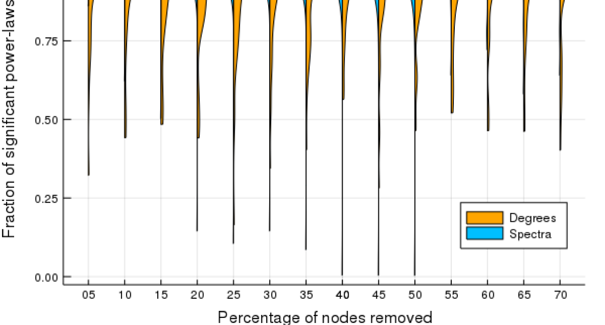 FIGURE 2: Forest Fire Sampling graphs generated using the preferential attachment model.
As discussed at length in this paper, preferential attachment has long been used to describe the reason why we find power-law distributions in the degrees of real world networks. There are many other empirical and theoretical studies on the presence of power-laws in spectra Chung et al. [2003a]; Goh et al. [2001]; Mihail and Papadimitriou [2002]; Eikmeier and Gleich [2017]. Given that many real-world networks should have power-laws in both the eigenvalues and the degrees, this suggests that one should be easier and more reliable to detect than the other. Our recent paper Eikmeier and Gleich [2017] gives evidence that power-laws are more likely to be present in the spectra than in degree distributions. An explanation for this observation may come from the way in which we obtain data, rather than a true feature of the data itself. Consider for a moment that the “real data” that is used in so many studies is not the full set of data. Instead, due to sampling or missing data the “real data” is actually some perturbation of the true set. If the underlying graph has both a power-law in the degrees and eigenvalues, then it is possible this observation just reflects the robustness of the eigenvalue power-law to the type of network sampling that occurred. There are many methods of sampling graphs, and studying properties of sampled graphs is a well-studied field Leskovec and Faloutsos [2006]; Stumpf and Wiuf [2005]; Stumpf et al. [2005]; Lovász et al. [1993]; Lee et al. [2006]; Ebrahimi et al. [2017]; Schoenebeck [2013].
[htbp]
![[Uncaptioned image]](/html/1904.12989/assets/images/FF.png)
![[Uncaptioned image]](/html/1904.12989/assets/images/DFS.png)
![[Uncaptioned image]](/html/1904.12989/assets/images/Rand_Edges.png) 35 TGPA graphs with power-law exponents between 2-5, sub-sampled in various ways. On the top, the graphs were sampled using a forest fire search on a random seed node; in the middle a depth first search; and on the bottom, by sampling random edges. Note that when there appears to be no violin plot (e.g. most spectra in DFS) that means 100 of the sampled graphs had significant power-laws. The horizontal lines give the median.
35 TGPA graphs with power-law exponents between 2-5, sub-sampled in various ways. On the top, the graphs were sampled using a forest fire search on a random seed node; in the middle a depth first search; and on the bottom, by sampling random edges. Note that when there appears to be no violin plot (e.g. most spectra in DFS) that means 100 of the sampled graphs had significant power-laws. The horizontal lines give the median.
Because the TGPA model produces graphs with reliable power-law exponents in both the degrees and spectra, as well as clustering, (Sections 6, 5) this makes it a good model to study this potential effect. We generated 35 TGPA graphs of size 5000 with theoretical degree power-law exponents between . For each graph, we detect that it has a statistically significant power-laws in both the degrees and spectra. The distributions were tested for power-laws using the method of Clauset et al. [2009]. We then perturbed each of the networks in three ways: In the first method we sampled random sets of edges of the graphs; in the second method we did a depth first search, starting at a random seed node; and third we did a forest fire sampling procedure from a random seed node (at each time step a fire “spreads” to each neighbor with some probability based on a burn rate). In each case, we ran the perturbation until a certain percentage of the nodes were obtained. And in each case we did the perturbation 50 times. The results of this experiment are shown in violin plots in Figure 8. Notice that the degree plots have a much larger spread in most cases, and the spectra almost always retains its power-law.
TGPA isn’t the only model with power-laws in both the degrees and eigenvalues (as we’ve proved about the GPA model in this manuscript). So we ask if we see these same sampling effects on other classes of models. When trying the same experiment on PA models, we don’t see as much variation between the degrees and spectra. See Figure 8 for an example of the forest fire sampling procedure. The other sampling procedures give similar results. We believe that the local structure of TGPA is necessary to see the effects of sampling. Note that we used the same size graphs, same number and number of samples as in the TGPA experiment.
9 Conclusions and Discussion
In this paper we presented the triangle generalized preferential attachment model, a graph model which incorporates direct triangle formulation into the preferential attachment model. Furthermore, we provided extensive analysis of this model, showing that the degree and spectral distributions fit power-law distributions. We also provided extended analysis of the generalized preferential attachment model found in Avin et al. [2017].
We further showed that triangle generalized preferential attachment has improved clustering coefficients over traditional preferential attachment models. Of course there are other models which exhibit higher order clustering that lack theoretical proofs of power-laws in both degrees and eigenvalues Eikmeier et al. [2018]; Holme and Kim [2002]; Lattanzi and Sivakumar [2009].
Our new model provides a useful platform for studying real-world network data. We found that it provided far more clustering in network data compared with the standard preferential attachment model. We further showed that if a graph has a significant power-law in both the spectra and degrees, under various sampling procedures (forest fire sampling, depth first search, and random edges), the spectral power-law remains much more frequently in sampled data. We provide this experiment as evidence for one possibly reason why we may see power-law distributions in the spectra of real networks more often than in the degrees. In the future, we plan to study further generalizations of higher-order preferential attachment graphs.
References
- Avin et al. [2017] C. Avin, Z. Lotker, Y. Nahum, and D. Peleg. Improved degree bounds and full spectrum power laws in preferential attachment networks. In Proceedings of the 23rd ACM SIGKDD International Conference on Knowledge Discovery and Data Mining, pp. 45–53. 2017.
- Barabási and Albert [1999] A.-L. Barabási and R. Albert. Emergence of scaling in random networks. Science, 286 (5439), pp. 509–512, 1999.
- Benson et al. [2017] A. Benson, D. F. Gleich, and L.-H. Lim. The spacey random walk: a stochastic process for higher-order data. SIAM Review, 59 (2), pp. 321–345, 2017. doi:10.1137/16M1074023.
- Benson et al. [2016] A. R. Benson, D. F. Gleich, and J. Leskovec. Higher-order organization of complex networks. Science, 353 (6295), pp. 163–166, 2016.
- Broido and Clauset [2019] A. D. Broido and A. Clauset. Scale-free networks are rare. Nature communications, 10 (1), p. 1017, 2019.
- Chung et al. [2006] F. Chung, F. R. Chung, F. C. Graham, L. Lu, K. F. Chung, et al. Complex graphs and networks, American Math. Soc., 2006.
- Chung et al. [2003a] F. Chung, L. Lu, and V. Vu. Eigenvalues of random power law graphs. Annals of Combinatorics, 7, pp. 21–33, 2003a.
- Chung et al. [2003b] ———. Spectra of random graphs with given expected degrees. Proceedings of the National Academy of Sciences, 100 (11), pp. 6313–6318, 2003b. arXiv:https://www.pnas.org/content/100/11/6313.full.pdf, doi:10.1073/pnas.0937490100.
- Clauset et al. [2009] A. Clauset, C. R. Shalizi, and M. Newman. Power-law distributions in empirical data. SIAM Review, 51 (4), pp. 661–703, 2009.
- Cooper and Frieze [2001] C. Cooper and A. M. Frieze. A general model of undirected web graphs. In European Symposium on Algorithms, pp. 500–511. 2001.
- Ebrahimi et al. [2017] R. Ebrahimi, J. Gao, G. Ghasemiesfeh, and G. Schoenbeck. How complex contagions spread quickly in preferential attachment models and other time-evolving networks. IEEE Transactions on Network Science and Engineering, 4 (4), pp. 201–214, 2017.
- Eikmeier and Gleich [2017] N. Eikmeier and D. F. Gleich. Revisiting power-law distributions in spectra of real world networks. In Proceedings of the 23rd ACM SIGKDD International Conference on Knowledge Discovery and Data Mining, pp. 817–826. 2017. doi:10.1145/3097983.3098128.
- Eikmeier et al. [2018] N. Eikmeier, A. S. Ramani, and D. F. Gleich. The hyperkron graph model for higher-order features. p. 1809.03488. 2018.
- Faloutsos et al. [1999] M. Faloutsos, P. Faloutsos, and C. Faloutsos. On power-law relationships of the internet topology. In SIGCOMM. 1999.
- Flaxman et al. [2005] A. Flaxman, A. Frieze, and T. Fenner. High degree vertices and eigenvalues in the preferential attachment graph. Internet Mathematics, 2 (1), pp. 1–19, 2005.
- Gjoka et al. [2010] M. Gjoka, M. Kurant, C. T. Butts, and A. Markopoulou. Walking in facebook: A case study of unbiased sampling of osns. In IEEE INFOCOM. 2010.
- Goh et al. [2001] K.-I. Goh, B. Kahng, and D. Kim. Spectra and eigenvectors of scale-free networks. Physical Review E, 64 (5), p. 051903, 2001.
- Golub and Van Loan [2013] G. H. Golub and C. F. Van Loan. Matrix Computations, The John Hopkins University Press, 4th edition, 2013.
- Grilli et al. [2017] J. Grilli et al. Higher-order interactions stabilize dynamics in competitive network models. Nature, 548, pp. 210–213, 2017. doi:10.1038/nature23273.
- Holme and Kim [2002] P. Holme and B. J. Kim. Growing scale-free networks with tunable clustering. Physical review E, 65 (2), p. 026107, 2002.
- Huberman [2001] B. A. Huberman. The Laws of the Web, The MIT Press, Cambridge, Massachusetts, 2001.
- Lattanzi and Sivakumar [2009] S. Lattanzi and D. Sivakumar. Affiliation networks. In Proceedings of the forty-first annual ACM symposium on Theory of computing, pp. 427–434. 2009.
- Lee et al. [2006] S. H. Lee, P.-J. Kim, and H. Jeong. Statistical properties of sampled networks. Physical Review E, 73 (1), p. 016102, 2006.
- Leskovec and Faloutsos [2006] J. Leskovec and C. Faloutsos. Sampling from large graphs. In Proceedings of the 12th ACM SIGKDD international conference on Knowledge discovery and data mining, pp. 631–636. 2006.
- Lovász et al. [1993] L. Lovász et al. Random walks on graphs: A survey. Combinatorics, Paul erdos is eighty, 2 (1), pp. 1–46, 1993.
- Medina et al. [2000] A. Medina, I. Matta, and J. Byers. On the origin of power laws in internet toplogies. ACM SIGCOMM Computer Communication Review, 30 (2), 2000.
- Meusel et al. [2015] R. Meusel, S. Vigna, O. Lehmberg, and C. Bizer. The graph structure in the web - analyzed on different aggregation levels. The Journal of Web Science, (1), pp. 33–47, 2015.
- Mihail and Papadimitriou [2002] M. Mihail and C. Papadimitriou. On the eigenvalue power law. In RANDOM ’02 Proceedings of the 6th International Workshop on Randomization and Approximation Techniques, pp. 254–262. 2002.
- Milo et al. [2002] R. Milo, S. Shen-Orr, S. Itzkovitz, N. Kashtan, D. Chklovskii, and U. Alon. Network motifs: Simple building blocks of complex networks. Science, 298 (5594), pp. 824–827, 2002. arXiv:http://science.sciencemag.org/content/298/5594/824.full.pdf, doi:10.1126/science.298.5594.824.
- Ostroumova et al. [2013] L. Ostroumova, A. Ryabchenko, and E. Samosvat. Generalized preferential attachment: tunable power-law degree distribution and clustering coefficient. In International Workshop on Algorithms and Models for the Web-Graph, pp. 185–202. 2013.
- Price [1976] D. D. S. Price. A general theory of bibliometric and other cumulative advantage processes. Journal of the American Society for Information Science, 27 (5), pp. 292–306, 1976. arXiv:https://onlinelibrary.wiley.com/doi/pdf/10.1002/asi.4630270505, doi:10.1002/asi.4630270505.
- Rosvall et al. [2014] M. Rosvall et al. Memory in network flows and its effects on spreading dynamics and community detection. Nat. Comm., 5 (4630), 2014.
- Saramäki and Kaski [2004] J. Saramäki and K. Kaski. Scale-free networks generated by random walkers. Physica A: Statistical Mechanics and its Applications, 341, pp. 80–86, 2004.
- Schoenebeck [2013] G. Schoenebeck. Potential networks, contagious communities, and understanding social network structure. In Proceedings of the 22nd international conference on World Wide Web, pp. 1123–1132. 2013.
- Stumpf and Wiuf [2005] M. P. Stumpf and C. Wiuf. Sampling properties of random graphs: the degree distribution. Physical Review E, 72 (3), p. 036118, 2005.
- Stumpf et al. [2005] M. P. Stumpf, C. Wiuf, and R. M. May. Subnets of scale-free networks are not scale-free: sampling properties of networks. Proceedings of the National Academy of Sciences, 102 (12), pp. 4221–4224, 2005.
- Toivonen et al. [2006] R. Toivonen, J.-P. Onnela, J. Saramäki, J. Hyvönen, and K. Kaski. A model for social networks. Physica A: Statistical Mechanics and its Applications, 371 (2), pp. 851–860, 2006.
- Traud et al. [2012] A. L. Traud, P. J. Mucha, and M. A. Porter. Social structure of facebook networks. Physica A, 391 (16), pp. 4165–4180, 2012. doi:10.1016/j.physa.2011.12.021.
- van der Hofstad [2016] R. van der Hofstad. Random graphs and complex networks: Volume 1. Cambridge Series in Statistical and Probabilistic Mathematics, Cambridge university press, 2016.
- Xu et al. [2016] J. Xu, T. L. Wickramarathne, and N. V. Chawla. Representing higher-order dependencies in networks. Science Advances, 2 (5), pp. e1600028–e1600028, 2016.
- Yin et al. [2018] H. Yin, A. R. Benson, and J. Leskovec. Higher-order clustering in networks. Physical Review E, 97 (5), p. 052306, 2018.
- Yule [1925] G. U. Yule. Ii.—a mathematical theory of evolution, based on the conclusions of dr. j. c. willis, f. r. s. Philosophical Transactions of the Royal Society of London B: Biological Sciences, 213 (402-410), pp. 21–87, 1925. doi:10.1098/rstb.1925.0002.
- Zadorozhnyi and Yudin [2015] V. Zadorozhnyi and E. Yudin. Growing network: models following nonlinear preferential attachment rule. Physica A: Statistical Mechanics and its Applications, 428, pp. 111–132, 2015.