Modeling the electronic structures of the ground and excited states of the ytterbium atom and the ytterbium dimer: A modern quantum chemistry perspective.

Abstract

We present a comprehensive theoretical study of the electronic structures of the Yb atom and the Yb₂ molecule, respectively, focusing on their ground and lowest-lying electronically excited states. Our study includes various state-of-the-art quantum chemistry methods such as CCSD, CCSD(T), CASPT2 (including spin–orbit coupling), and EOM-CCSD as well as some recently developed pCCD-based approaches and their extensions to target excited states. Specifically, we scan the lowest-lying potential energy surfaces of the Yb2 dimer and provide a reliable benchmark set of spectroscopic parameters including optimal bond lengths, vibrational frequencies, potential energy depths, and adiabatic excitation energies. Our in-depth analysis unravels the complex nature of the electronic spectrum of Yb2, which is difficult to model accurately by any conventional quantum chemistry method. Finally, we scrutinize the bi-excited character of the first ${}^{1}\Sigma_{g}^{+}$ excited state and its evolution along the potential energy surface.

INTRODUCTION

The divalent ytterbium atom has in recent years garnered significant attention thanks to its many uses in cold atom physics. It has a non-magnetic ¹S₀ ground state and several useful optical transitions: the strong ¹S${}_{0}\leftrightarrow^{1}$P₁ line can be used for Zeeman slowing, whereas the narrow (181 kHz) intercombination ¹S${}_{0}\leftrightarrow^{3}$P₁ line can be used to directly laser cool Yb atoms to microkelvin temperatures ¹. Yb has seven stable isotopes: two fermions (171 and 173 with nuclear spins of $1/2$ and $5/2$, respectively) and five bosons (168, 170, 172, 174, and 176) that lack nuclear spin. The rich isotope structure makes it possible to mass-tune the atomic interactions ² and facilitates a wide array of possible quantum-degenerate gases ^{3, 4, 5, 6}. The doubly forbidden ¹S₀$\leftrightarrow$³P₀ transition lies at the heart of optical atomic clocks ⁷ which are among the most precise physical instruments known to mankind. For example, an ytterbium clock has recently been demonstrated to enable geopotential measurements with an accuracy below a centimetre ⁸. The long lived ³P₀ clock states also find use in quantum simulations using Yb atoms ⁹.

The long range interactions in the Yb dimer have been probed extensively by high resolution photoassociation spectroscopy (PAS) ¹⁰ near the narrow ¹S₀$\leftrightarrow$³P₁ intercombination line. The excited ¹S₀+³P₁ ($0_{u}^{+}$) ^{11, 12} state has been probed by single color PAS and provided the van der Waals $C_{6}$ coefficient and an improved value of the atomic ³P₁ lifetime. Two-color PAS of ground state $0_{g}^{+}$ vibrational levels ^{2, 13} delivered accurate information about the cold scattering properties of Yb, most notably the $s$-wave scattering lengths for all isotopic combinations. Additionally, intercombination line PAS has provided insight into such exotic physical phenomena as subradiant $1_{g}$ states ¹⁴ and hyperfine-induced purely-long-range states ¹⁵. PA lines near the intercombination line also gives experimentalists the capacity to alter the scattering properties of ultracold Yb atoms optically through the optical Feshbach resonance mechanism ^{16, 17, 12, 18}.

Other excited states of Yb₂ have also been probed in ultracold atom experiments. The $s$-wave scattering length in the ¹S₀+³P₀ ($0_{u}^{-}$) state in ¹⁷⁴Yb₂ has been determined through clock spectroscopy of Bose–Einstein condensates trapped in 3D optical lattices ^{19, 20}. Based on these measurements the positions of near-threshold molecular clock states could be determined ²¹. Orbital Feshbach resonances have been utilized to produce strong correlations ²² in a degenerate Fermi gas of ¹⁷³Yb atoms and create a novel type of Feshbach molecules ²³. Collisions of atoms in the ground and metastable ³P₂ states have also been considered: magnetic Feshbach resonances ²⁴ and Feshbach molecules ²⁵ have been observed experimentally. Feshbach resonances in this pair of states have been shown to exhibit quantum chaos ²⁶.

Finally, Yb offers excellent opportunities for tests of fundamental physics. It – uniquely – possesses two independent clock transitions with an unusually high sensitivity to possible variations of the fine structure constant ²⁷. Open-shell molecules involving Yb, like RbYb or LiYb can be used in searches for the electric dipole moment of the electron (eEDM) ²⁸. Thanks to its simple structure, the ground state Yb dimer is an excellent testing ground for the search for new short scale gravitylike forces ²⁹, temporal variations of the proton-to-electron mass ratio ³⁰, or beyond-Born-Oppenheimer effects ¹³. An “optical molecular clock”  ²¹ utilizing forbidden $J=0\leftrightarrow 0$ transitions between the ground $(1)\,0_{g}^{+}$ and clock $(1)\,0_{u}^{-}$ states in Yb₂ could provide energy level measurements at an accuracy so far unprecedented in molecular spectroscopy.

Despite these advancements, our knowledge of the ground and excited state electronic structures of the Yb₂ dimer and the resulting interaction potentials remain scarce. The detailed knowledge of molecular potential energy curves would be the first step towards the production of deeply bound ultracold molecules via stimulated Raman adiabatic passage (StiRAP) ³¹. Unfortunately, the reliable quantum chemical modeling of the Yb₂ dimer is not straightforward and poses a remarkable challenge for present-day quantum chemistry to provide accurate interaction potentials for both the ground and excited states. The large number of correlated electrons combined with a sizable all-electron basis set makes the theoretical modeling of Yb2 computationally very demanding. Moreover, the Yb atom (Z=70) falls into the class of heavy elements and thus requires a relativistic description of the electronic motion. While for a qualitative study it is sufficient to account for scalar relativistic effects only, spin–orbit coupling has to be included in calculations for a quantitative analysis as well as for electron excitation energies. The rather complex interplay between electron correlation and relativistic effects ³² impedes routine quantum chemical calculations on the Yb2 dimer.

To date, the spin–free coupled cluster ground state interaction potential was investigated by Buchachenko et al. ³³, while reliable van der Waals C_6 coefficients for ground and selected excited states were calculated by Safronova et al. ³⁴ and Porsev et al. ³⁵, respectively. The very first attempt to understand and model the low-lying part of the electronic spectrum of Yb₂ has been already performed in 1998 by Wang and Dolg ³⁶. In their multi-reference configuration interaction study, they considered potential energy curves resulting from electron excitations from the occupied $\sigma_{u}$ and $\sigma_{g}$ to the virtual $\pi_{u}$, $\pi_{g}$, $\sigma_{g}$, and $\sigma_{u}$ molecular orbitals. Taking into account recent advances in method development for ground and excited states, higher-quality basis sets, and the increase in computation power, it is now possible to deepen our knowledge on the ground and electronic excited states of Yb2 and provide more reliable benchmark data for potential energy curves (both ground and excited states) that can be exploited in future experimental manipulations of Yb2. The main goal of our work is, thus, to provide a reliable description of the ground and electronic excited states potential energy surfaces of the Yb2 dimer using modern wave function-based quantum chemistry methods.

METHODOLOGY

Basis sets and scalar relativity

In all our calculations, we used the all-electron atomic natural orbital relativistic correlation consistent (ANO-RCC) basis sets available in the OpenMolcas program package , optimized specifically for the 2-nd order Douglas–Kroll–Hess (DKH) Hamiltonian ³⁷. We employed the triple-$\zeta$ (TZ), quadruple-$\zeta$ (QZ), and “large” quality basis sets with the following contraction schemes: $25s22p15d11f4g2h\rightarrow 8s7p4d3f2g$, $25s22p15d11f4g2h\rightarrow 9s8p5d4f3g$, $25s22p15d11f4g2h\rightarrow 11s10p8d7f4g$, respectively. The most accurate calculations for the ground state included a fully uncontracted ANO-RCC basis set and the 5-th order DKH Hamiltonian. We should note that the quality of the calculated potential energy surfaces is not affected by the order of the DKH transformation. Thus, for all other electronic structure methods, scalar relativistic effects were accounted for by the second order Douglas–Kroll–Hess Hamiltonian (DKH2) ^{38, 39}.

pCCD-based methods

All pair Coupled Cluster Doubles (pCCD) ^{40, 41} calculations, also known as the Antisymmetric Product of 1-reference orbital Geminal (AP1roG), were performed using our locally developed PIERNIK ⁴² software package. The pCCD ansatz can be written as

$$|{\rm pCCD}\rangle=\exp\left(\sum_{i=1}^{\rm occ}\sum_{a=1}^{\rm virt}t_{i}^{a}a_{a}^{\dagger}a_{\bar{a}}^{\dagger}a_{\bar{i}}a_{i}\right)|0\rangle=e^{T_{\rm p}}|0\rangle,$$ (1)

where $a^{\dagger}_{p}$ and $a_{p}$ ($a^{\dagger}_{\bar{p}}$ and $a_{\bar{p}}$) are the electron creation and annihilation operators for $\alpha$ ($\beta$) electrons and $|0\rangle$ is some independent-particle wave function (for instance, the Hartree–Fock (HF) determinant). In eq. (1), $\{t_{i}^{a}\}$ are the electron-pair amplitudes and $\hat{T}_{\rm p}=\sum_{i=1}^{\rm occ}\sum_{a=1}^{\rm virt}t_{i}^{a}a_{a}^{\dagger}a_{\bar{a}}^{\dagger}a_{\bar{i}}a_{i}$ is the electron-pair excitation operator that excites an electron pair from an occupied orbital $(i\bar{i})$ to a virtual orbital $(a\bar{a})$ with respect to $|0\rangle$. In all pCCD and post-pCCD calculations, we used different sets of orbitals: canonical Hartree–Fock orbitals and variationally optimized pCCD orbitals (denoted as voo-pCCD) ^{43, 44, 45}. Furthermore, voo-pCCD calculations were constraint to the D_2h and C_2v point group symmetry, respectively. The missing dynamical energy correction on top of pCCD/voo-pCCD was included via a linearized coupled cluster correction ⁴⁶, denoted as pCCD-LCCSD.

Moreover, three variants of the equation of motion (EOM) coupled cluster model to target excited states within the pCCD formalism were investigated. First, the EOM formalism was directly applied on top of the pCCD reference. Single excitations were included a posteriori in the EOM ansatz, that is, the linear excitation operator of the EOM formalism is limited to pair and single excitations. This approach is denoted as EOM-pCCD+S ^{47, 48}. The second model includes single excitations also in the coupled cluster reference function. These single excitations are included on top of the pCCD reference function. This method is labeled as pCCD-CCS, while the excited state extension is abbreviated as EOM-pCCD-CCS. Finally, in the most accurate EOM variant, the pCCD reference was replaced by the pCCD-LCCSD function, resulting in the EOM-pCCD-LCCSD approach ^{49, 50}.

EOM-CCSD/CCSD(T)

All CCSD(T) ⁵¹ and EOM-CCSD ⁵² calculations were carried out in the Molpro2012 software package ^{53, 54, 55, 56} using D_2h point group symmetry.

CASSCF/SO-CASPT2

The Complete Active Space Self Consistent Field (CASSCF) ^{57, 58} calculations and Complete Active Space Second-order Perturbation Theory (CASPT2) ^{59, 60, 61} calculations were performed in the D_2h point group symmetry using the OpenMolcas (version 17.0) software package ^{62, 63, 64, 65}. The CASSCF wave functions were used to calculate multistate CASPT2 energy corrections, where the ionization potential-electron affinity (IPEA) shifted H₀ Hamiltonian ⁶⁶ was applied with an imaginary shift set to 0.25. The spin–orbit (SO) interaction effects (in the Atomic Mean Field Approximation ^{67, 68, 69}) were calculated using the Restricted Active Space State Interaction (RASSI) approach, ⁷⁰ where the energy correction due to dynamical correlation was included in an approximate manner by dressing the diagonal elements of the spin-orbit Hamiltonian by the CASPT2 energies. Throughout this work, we utilized the state averaged CASSCF approach combined with the subsequent RASSI/SO calculations with the same active space sizes as in CASSCF. In the Yb atomic calculations, we employed two active space variants: CAS(2,4)SCF with the 6s and 6p orbitals correlated and CAS(2,9)SCF augmented by the additional 5d orbitals. For the Yb2 molecule, we performed CAS(4,8)SCF calculations which comprised occupied σ_u (Yb 6s) and σ_g (Yb 6s) orbitals as well as virtual σ_g (Yb 6p_z), σ_u (Yb 6p_z), π_u (Yb 6p_x/p_y), and π_g (Yb 6p_x/p_y) molecular orbitals.

Fitting procedure

All potential energy curves were obtained from a polynomial fit of 8-th order. The corresponding spectroscopic constants (equilibrium bond length (r_e) and harmonic vibrational frequency ($\omega_{\rm e}$)) were calculated based on those fitted potential energy curves. Specifically, the harmonic vibrational frequencies ($\omega_{\rm e}$) were determined numerically using the five-point finite difference stencil ⁷¹ and the average mass of ytterbium, that is, 173.045. ⁷² The potential energy depth (D_e) was evaluated as the difference between the atomic limit and the minimum energy of a given potential energy curve. Note that in pCCD-based calculations employing D_2h point group symmetry the dissociation energies were estimated by adding the corresponding atomic excitation energies to the dissociation limit of the dimer calculation. This step had to be performed due to size-consistency problems in the pCCD reference function. If the orbitals are allowed to relax freely, the size-consistency error is eliminated and the dissociation limits of the dimer calculation numerically agree with the atomic ground and excited state energies.

RESULTS and DISCUSSION

The electronic structure of the ytterbium atom

Ytterbium is a closed-shell atom described by the ground-state ^1S_0 term. Its valence electronic configuration is characterized by the fully occupied 4f and 6s subshells and the low-lying unoccupied 5p, 5d, and 7s subshells. Despite its closed-shell electronic nature, the ytterbium atom has a rather complex electronic structure, which manifests itself in close-lying potential energy levels ^{72, 73}. Specifically, in the range of 17 000 to 50 000 cm^-1, there is a large number of quasi-degenerate states that are characterized by electron transfer not only from the occupied 6s to the unoccupied 5p, 5d, 7s, and 8s orbitals, but also from the occupied 4f (7-fold) semi-core orbitals. This peculiar electronic structure leads to a large number of low-lying excited states and a very dense electronic spectrum, for some of which atomic term symbols are difficult to assign ^{72, 73}.

In this work, we focus on the low-lying energy levels of the Yb atom arising from the occupied 6s to the unoccupied 5p and 5d orbitals. Specifically, we use the experimentally determined energy levels available in Refs. 72, 73 as a starting point to assess the accuracy of different quantum chemistry methods. Since not all quantum chemistry methods used in this work are directly applicable to triplet excited states (EOM-based approaches), we first focus on the lowest-lying ^1D ($6s\rightarrow 5d$) and ^1P ($6s\rightarrow 6p$) energy levels of Yb. The corresponding results are summarized in Table 1.

Spin–free levels $[$cm${}^{-1}]$ Main config. Term EOM CAS(2,9) Exp.^∗ pCCD+S pCCD-CCS pCCD-LCCSD CCSD CASSCF CASPT2 Ref. 72 4f¹⁴6s6p ¹P 29 131 29 127 26 452 25 826 24 672 25 007 24 964 4f¹⁴6s5d ¹D 29 414 29 355 29 303 30 182 27 840 27 574 27 628

• ^∗ The empirical positions 24 964 cm^-1 and 18 903 cm^-1 respectively of spin-free ¹P and ³P states were determined from experimental positions of ¹P₁ and ³P_0,1,2 states using the spin-orbit Hamiltonian in Ref. 74 and take into account the mutual repulsion between ³P₁ and ¹P₁ states. Analogously, the empirical positions of spin-free ¹D and ³D states are 27 628 cm^-1 and 24 958 cm^-1, respectively, and account for the repulsion between the ¹D₂ and ³D₂ states.

Table 1: Singlet electronic energy levels of the Yb atom calculated from different quantum chemistry methods using the TZ-ANO-RCC basis set (in cm^-1). The energy of the ¹S ground state (electronic configuration 4f¹⁴6s²) equals zero for all theoretical models and experiment.

All excited state methods correctly place the ¹P state below ¹D; nonetheless, the splitting between these two states differs for all investigated approaches. All considered EOM-based theories overestimate the energy of the ¹D level by approximately 2 000 cm^-1. The ¹P state is rather accurately predicted by the standard EOM-CCSD method, followed by EOM-pCCD-LCCSD. For more simplified EOM models, however, larger deviations from the reference value are observed (differences amount to 3 000 cm^-1). This results in underestimated energy splittings between the ¹P and ¹D terms. On the other hand, spin–free CASSCF and CASPT2 electronic spectra match very well the experimental energy levels mentioned in Table 1. The overall deviations do not exceed 300 and 100 cm^-1 for CASSCF and CASPT2, respectively.

The Yb energy levels obtained from SO-CAS(2,4)PT2 and SO-CAS(2,9)PT2 combined with various basis set sizes are presented in Tables 2 and 3. Both active spaces qualitatively reproduce the experimental energy levels of the Yb atom with respect to the energetic order and magnitude of spin-orbit splittings. The largest differences between the CAS(2,4) and CAS(2,9) variants are observed for the ¹P state, which is underestimated by about 2 000 cm^-1 in the smaller CAS. This shift in energy highlights the importance of unoccupied d-type orbitals in post-Hartree–Fock calculations, similar to the double d-shell effect in 3d transition metal chemistry. ⁷⁵ In both active space calculations, dynamic energy corrections seem to be important and amount to 500–2 000 cm^-1 for a given energy level. Finally, we should note that the quality of excitation energies in the Yb atom seems to be rather insensitive to the basis set quality. Only minor changes in the order of states are observed and amount to a few hundreds of cm^-1 (cf. Table 3). These observations point to a well-balanced, good quality ANO-RCC basis set for valence atomic properties of the Yb atom.

Basis Main config. Term Spin–free levels $[$cm${}^{-1}]$ Spin–orbit levels $[$cm${}^{-1}]$ CAS(2,4)SCF CASPT2 Exp.^∗ 72 J SO-CASPT2 Exp. 72 TZ-ANO-RCC 4f¹⁴6s6p ³P 16 304 17 123 18 903 0 15 965 17 288 1 16 523 17 992 2 17 704 19 710 4f${}^{1}4$6s6p ¹P 29 608 28 011 24 964 1 28 041 25 068 QZ-ANO-RCC 4f¹⁴6s6p ³P 16 315 17 207 18 903 0 16 074 17 288 1 16 628 17 992 2 17 779 19 710 4f${}^{1}4$6s6p ¹P 28 966 27 430 24 964 1 27 453 25 068 large-ANO-RCC 4f¹⁴6s6p ³P 16 315 17 256 18 903 0 16 120 17 288 1 16 675 17 992 2 17 828 19 710 4f¹⁴6s6p ¹P 28 512 27 025 24 964 1 27 046 25 068

• ^∗ See the footnote below Table 1.

Table 2: Electronic energy levels of the Yb atom calculated from the SO-CAS(2,4)PT2 approach and different quality ANO-RCC basis sets (in cm^-1). The energy of the ¹S ground state (electronic configuration 4f¹⁴6s²) equals zero for all theoretical models and experiment.

Basis Main config. Term Spin–free levels $[$cm${}^{-1}]$ Spin–orbit levels $[$cm${}^{-1}]$ CAS(2,4)SCF CASPT2 Exp.^∗ 72 J SO-CASPT2 Exp. 72 TZ-ANO-RCC 4f¹⁴6s6p ³P 15 497 16 694 18 903 0 15 528 17 288 1 16 064 17 992 2 17 276 19 710 4f¹⁴6s5d ³D 26 895 25 684 24 958 1 25 149 24 489 2 25 443 24 752 3 26 040 25 271 4f${}^{1}4$6s6p ¹P 24 672 25 007 24 964 1 25 053 25 068 4f${}^{1}4$6s5d ¹D 27 840 27 574 27 628 2 27 690 27 678 QZ-ANO-RCC 4f¹⁴6s6p ³P 15 416 16 862 18 903 0 15 720 17 288 1 16 249 17 992 2 17 433 19 710 4f¹⁴6s5d ³D 26 573 25 124 24 958 1 24 614 24 489 2 24 899 24 752 3 25 474 25 271 4f${}^{1}4$6s6p ¹P 24 275 24 793 24 964 1 24 834 25 068 4f${}^{1}4$6s5d ¹D 27 485 27 142 27 628 2 27 265 27 678 large-ANO-RCC 4f¹⁴6s6p ³P 15 381 16 997 18 903 0 15 870 17 288 1 16 399 17 992 2 17 560 19 710 4f¹⁴6s5d ³D 26 414 24 423 24 958 1 23 909 24 489 2 24 202 24 752 3 24 747 25 271 4f¹⁴6s6p ¹P 24 170 24 848 24 964 1 24 888 25 068 4f¹⁴6s5d ¹D 27 191 26 373 27 628 2 26 500 27 678

• ^∗ See the footnote below Table 1.

Table 3: Electronic energy levels of the Yb atom calculated from the SO-CAS(2,9)PT2 approach and different quality ANO-RCC basis sets (in cm^-1). The energy of the ¹S ground state (electronic configuration 4f¹⁴6s²) equals zero for all theoretical models and experiment.

Towards a reliable and accurate ground state potential energy surface for the Yb2 dimer

When the two Yb atoms approach each other, they create a weakly-bonded, van der Waals-type complex. ^{76, 36, 77, 33} It is well-known that such weakly-bonded compounds tend to be extremely sensitive to the quality of the atomic basis set and the (approximate) dynamic energy correction. ⁷⁸ Thus, we first scrutinize the ground state potential energy surface obtained from the CCSD(T) approach before benchmarking various electron correlation methods for both ground and excited states.

Reference ground-state potential energy curve

Table 4 summarizes the influence of the number of correlated electrons on the quality of the CCSD and CCSD(T) potential energy surfaces, respectively, including their spectroscopic constants (optimal bond lengths ($\mathrm{r_{e}}$), harmonic vibrational frequencies ($\omega_{e}$), and potential energy depths ($\mathrm{D_{e}}$)). To minimize the basis set superposition error ⁷⁹ we employed the all-electron uncontracted ANO-RCC basis set. Our calculations suggest that it is necessary to correlate all occupied orbitals starting from the fourth atomic shell of the Yb atom (see Table 4), that is, 84 electrons of the Yb dimer have to be correlated in a calculation. Correlating additional core electrons does not considerably change the spectroscopic constants of Yb2. Our most accurate CCSD(T) prediction yields an optimal bond length of $\mathrm{r_{e}}=8.814$ bohr, a harmonic vibrational frequencies of $\omega_{e}=21$ cm^-1, and a potential energy depth of $\mathrm{D_{e}}=579$ cm^-1. The computed harmonic vibrational frequency matches the experimental value of 22 cm^-1 measured by Goodfriend ⁸⁰. It is important to note that restricting the number of correlated electrons to 32 or less shifts the optimal bond length towards longer inter-atomic distances and overestimates the potential energy depth. Neglecting contributions from triply-excited determinants (as in CCSD) elongates the optimal bond length by approximately 0.4 bohr and lowers the vibrational frequencies and potential energy depth. The latter is most significantly affected by the lack of triple excitations in the cluster operator, where the differences in $D_{e}$ between CCSD and CCSD(T) amount to 250–300 cm^-1 (a difference of approximately 40%, see also Table 4). Analysis of the t₁ diagnostic ⁸¹ in CCSD along potential energy surface shows a single-reference nature of the Yb₂ ground-state (values in the order of 0.02). Finally, we should mention that our new best estimate for the potential energy depth, $\mathrm{D_{e}}=579$ cm^-1, is lower than the recently reported value of $\mathrm{D_{e}}=786$ cm^-1 by Mosyagin and coworkers ⁸², who employed a smaller basis set and different approaches to electron correlation and relativistic effects.

method correlated occupied orbitals $\mathrm{N_{e}}$ $\mathrm{r_{e}[a_{0}]}$ $\mathrm{\omega_{e}[cm^{-1}]}$ $\mathrm{D_{e}[cm^{-1}]}$ CCSD 6s 4 9.438 17 365 CCSD 5s, 5p, 6s 20 9.373 16 342 CCSD 4f, 6s 32 9.293 16 345 CCSD 5p, 4f, 6s 44 9.281 16 328 CCSD 5s, 5p, 4f, 6s 48 9.277 16 336 CCSD 4s, 4p, 4d, 5s, 5p, 4f, 6s 84 9.260 16 336 CCSD 3s, 3p, 3d, 4s, 4p, 4d, 5s, 5p, 4f, 6s 120 9.266 16 336 CCSD 1s, 2s, 2p, 3s, 3p, 3d, 4s, 4p, 4d, 5s, 5p, 4f, 6s 140 9.265 16 336 CCSD(T) 6s 4 9.050 22 645 CCSD(T) 5s, 5p, 6s 20 8.968 21 592 CCSD(T) 4f, 6s 32 8.874 21 591 CCSD(T) 5p, 4f, 6s 44 8.822 21 579 CCSD(T) 5s, 5p, 4f, 6s 48 8.810 21 585 CCSD(T) 4s, 4p, 4d, 5s, 5p, 4f, 6s 84 8.815 21 580 CCSD(T) 3s, 3p, 3d, 4s, 4p, 4d, 5s, 5p, 4f, 6s 120 8.814 21 579 CCSD(T) 1s, 2s, 2p, 3s, 3p, 3d, 4s, 4p, 4d, 5s, 5p, 4f, 6s 140 8.814 21 579

Table 4: CCSD and CCSD(T) spectroscopic constants for the Yb2 X $\mathrm{{}^{1}\Sigma_{g}^{+}}$ state using uncontracted ANO-RCC basis set and a varying number of active (occupied) orbitals and thus correlated electrons. N${}_{\text{corr}}$ denotes the number of correlated electrons, $\mathrm{r_{e}}$ the equilibrium bond length, $\mathrm{\omega_{e}}$ the vibrational frequency, and $\mathrm{D_{e}}$ the potential depth, respectively. The occupied orbitals not included in the set of correlated orbitals (second column) were kept frozen during CCSD(T) calculations. All virtual orbitals were correlated.

Assessing the accuracy of conventional and unconventional quantum chemistry approaches in modeling the ground state potential energy surface

The CCSD potential energy curve can be used as a reference to evaluate the reliability of simplified coupled cluster methods that include at most double excitations. Table 5 lists the spectroscopic constants obtained from various quantum chemistry methods and a given basis set. Including an LCCSD dynamic energy correction on top of the pCCD reference wave-function is indispensable for obtaining qualitatively correct bond lengths. Furthermore, the potential energy depth heavily depends on the type of orbitals used in the pCCD reference calculations (canonical Hartree–Fock or variationally optimized orbitals imposing C_2v and D_2h point group symmetry). The best agreement of all pCCD-based methods with CCSD (as well as with CCSD(T) reference) data is obtained when the point group symmetry is lowered and the orbitals are thus allowed to (partially) localize in the dimer calculation. Note that orbital optimization in pCCD typically involves localization. ^{83, 84} CAS(4,8)PT2 results in overly bond lengths and underestimated low vibrational frequencies compared to CCSD calculations (employing the same basis set). Increasing the basis set size in CAS(4,8)PT2 improves the agreement between CCSD and CASPT2 data. The slower convergence of the second-order perturbation theory approach with basis set size for weakly interacting systems is not surprising and has been reported earlier in the literature ⁸⁵. As to be expected, inclusion of spin–orbit coupling does not significantly affect the quality of the CAS(4,8)PT2 ground-state potential energy curve. To this end, we can conclude that both the pCCD-LCCSD($C_{2v}$) and CAS(4,8)PT2 methods are promising alternatives for modeling excited state potential energy curves in the Yb₂ dimer.

method $\mathrm{N_{e}}$ basis $\mathrm{r_{e}[a_{0}]}$ $\mathrm{\omega_{e}[cm^{-1}]}$ $\mathrm{D_{e}[cm^{-1}]}$ CCSD 48 TZ-ANO-RCC 8.684 24 956 pCCD 48 TZ-ANO-RCC 10.004 14 361 pCCD($D_{2h}$) 48 TZ-ANO-RCC 8.604 27 1 046 pCCD($C_{2v}$) 48 TZ-ANO-RCC 13.674 22 22 pCCD-LCCSD 48 TZ-ANO-RCC 8.102 36 1 875 pCCD-LCCSD($D_{2h}$) 48 TZ-ANO-RCC 7.852 42 2 609 pCCD-LCCSD($C_{2v}$) 48 TZ-ANO-RCC 8.467 26 785 CAS(4,8)PT2 4/32 TZ-ANO-RCC 11.381 13 280 CAS(4,8)PT2 4/32 QZ-ANO-RCC 10.998 11 256 CAS(4,8)PT2 4/32 large-ANO-RCC 8.837 19 369 SO-CAS(4,8)PT2 4/32 TZ-ANO-RCC 10.751 11 221 SO-CAS(4,8)PT2 4/32 QZ-ANO-RCC 10.463 9 259 SO-CAS(4,8)PT2 4/32 large-ANO-RCC 8.519 24 409

Table 5: Spectroscopic constants for the Yb2 X $\mathrm{{}^{1}\Sigma_{g}^{+}}$ state from different quantum chemistry methods. N${}_{\text{corr}}$ denotes the number of correlated electrons, $\mathrm{r_{e}}$ equilibrium bond length, $\mathrm{\omega_{e}}$ vibrational frequency, and $\mathrm{D_{e}}$ potential depth, respectively.

Yb2 excited-state properties

Examination of the electronic structure of the Yb atom points to the importance of the 4$f$, 6$s$, 6$p$, and 5$d$ atomic orbitals in the electronic spectrum of Yb₂. Including all these orbitals in active space calculations is prohibitive and some compromise has to be made. A reasonable choice would be to correlate only the 6$s$, 6$p$, and 5$d$ atomic orbitals in molecular Yb₂ calculations, that is, performing CAS(4,18)SCF calculations. Unfortunately, such an active space is not stable along the potential energy surface, where smooth potential energy curves for all excited states of interest cannot be optimized due to technical difficulties. As a consequence, we had to reduce the number of active orbitals and neglected the contributions from 5$d$ orbitals by moving them outside the CAS space (into the external space). This results in our CAS(4,8)SCF model that is further used as reference for all Yb₂ excited states potential energy curves. We should stress that the same active space was used in previous ECP/MRCI calculations ³⁶.

Reference spin-free electronic spectrum

Table 6 collects all spin–free spectroscopic constants obtained from CAS(4,8)PT2 using different sizes for the atomic basis set. Similar to the ground state calculations, the CAS(4,8)PT2 spectroscopic constants converge very slowly with basis set size. In general, incrementing the basis set size shortens bond lengths, marginally increases vibrational frequencies, deepens potential energy depths, and lowers the adiabatic excitation energies. The CAS(4,8)PT2 results obtained using the TZ-ANO-RCC basis set qualitatively match the ECP/MRCI ³⁶ spectroscopic constants (cf. Table 6). The largest discrepancies are observed for the higher-lying ${}^{1}\Pi_{u}$ and ${}^{1}\Sigma_{g}^{+}$ excited states, where the differences in excitation energies amount to few thousand wave numbers. The agreement between ECP/MRCI and all-electron CAS(4,8)PT2 spectroscopic parameters decreases for larger basis sets, indicating the need for decent basis set sizes to reliably describe excited-state potential energy surfaces of Yb₂. The discrepancies between ECP/MRCI and CAS(4,8)PT2 can be attributed to the different treatment of scalar relativistic and electron correlation effects in both approaches. One should keep in mind that any truncated CI approach, such as MRCI, is not rigorously size-extensive and size-consistent, while CASPT2 is, in general, size-extensive and approximately size-consistent. Thus, we believe that our CAS(4,8)PT2 results can be considered as new reference data for the excited potential energy curves of the Yb₂ dimer. We further hope that future experiments on laser induced fluorescence will help to resolve this ambiguity.

State	basis	$\mathrm{r_{e}[a_{0}]}$	$\mathrm{\omega_{e}[cm^{-1}]}$	$\mathrm{D_{e}[cm^{-1}]}$	$\mathrm{T_{e}[cm^{-1}]}$	Dissociation limit
${}^{3}\Pi_{g}$	TZ-ANO-RCC	6.955	69	6 255	11 147	$\mathrm{{}^{1}S+^{3}P}$
	QZ-ANO-RCC	6.890	69	6 640	10 823	$\mathrm{{}^{1}S+^{3}P}$
	large-ANO-RCC	6.794	73	7 566	10 059	$\mathrm{{}^{1}S+^{3}P}$
	ECP(MRCI) 36	6.680	77	8 065	12 421	$\mathrm{{}^{1}S+^{3}P}$
${}^{1}\Pi_{g}$	TZ-ANO-RCC	6.751	79	15 776	12 514	$\mathrm{{}^{1}S+^{1}P}$
	QZ-ANO-RCC	6.688	77	15 684	12 002	$\mathrm{{}^{1}S+^{1}P}$
	large-ANO-RCC	6.612	80	16 364	11 030	$\mathrm{{}^{1}S+^{1}P}$
	ECP(MRCI) 36	6.546	84	14 841	13 389	$\mathrm{{}^{1}S+^{1}P}$
${}^{3}\Sigma_{u}^{+}$	TZ-ANO-RCC	7.697	56	4 141	13 261	$\mathrm{{}^{1}S+^{3}P}$
	QZ-ANO-RCC	7.636	57	4 493	12 970	$\mathrm{{}^{1}S+^{3}P}$
	large-ANO-RCC	7.578	61	5 315	12 310	$\mathrm{{}^{1}S+^{3}P}$
	ECP(MRCI) 36	7.559	58	5 162	15 325	$\mathrm{{}^{1}S+^{3}P}$
${}^{3}\Pi_{u}$	TZ-ANO-RCC	8.835	21	425	16 978	$\mathrm{{}^{1}S+^{3}P}$
	QZ-ANO-RCC	8.693	22	522	16 942	$\mathrm{{}^{1}S+^{3}P}$
	large-ANO-RCC	8.374	31	802	16 824	$\mathrm{{}^{1}S+^{3}P}$
	ECP(MRCI) 36	8.343	24	1 048	19 438	$\mathrm{{}^{1}S+^{3}P}$
${}^{1}\Sigma_{u}^{+}$	TZ-ANO-RCC	7.513	48	8 774	19 516	$\mathrm{{}^{1}S+^{1}P}$
	QZ-ANO-RCC	7.307	52	8 906	18 781	$\mathrm{{}^{1}S+^{1}P}$
	large-ANO-RCC	7.078	60	10 405	16 989	$\mathrm{{}^{1}S+^{1}P}$
	ECP(MRCI) 36	7.359	53	7 824	20 406	$\mathrm{{}^{1}S+^{1}P}$
${}^{1}\Pi_{u}$	TZ-ANO-RCC	7.258	71	5 595	22 695	$\mathrm{{}^{1}S+^{1}P}$
	QZ-ANO-RCC	7.273	67	5 455	22 232	$\mathrm{{}^{1}S+^{1}P}$
	large-ANO-RCC	7.223	69	6 124	21 270	$\mathrm{{}^{1}S+^{1}P}$
	ECP(MRCI) 36	7.319	56	1 936	26 294	$\mathrm{{}^{1}S+^{1}P}$
${}^{1}\Sigma_{g}^{+}$	TZ-ANO-RCC	7.664	68	5 111	23 179	$\mathrm{{}^{1}S+^{1}P}$
	QZ-ANO-RCC	7.461	71	5 008	22 679	$\mathrm{{}^{1}S+^{1}P}$
	large-ANO-RCC	7.856	49	4 727	22 667	$\mathrm{{}^{1}S+^{1}P}$
	ECP(MRCI) 36	7.529	58	1 613	26 616	$\mathrm{{}^{1}S+^{1}P}$

Table 6: Adiabatic spin–free electronic spectrum of Yb2 from CAS(4,8)PT2 using different ANO-RCC basis sets. $\mathrm{r_{e}}$ denotes the equilibrium bond length, $\mathrm{\omega_{e}}$ vibrational frequency, $\mathrm{D_{e}}$ potential depth, and $\mathrm{T_{e}}$ adiabatic excitation energy, respectively. The ${}^{3}\Sigma_{g}^{+}$ state does not have a minimum and thus its spectroscopic constants are not calculated.

Singlet excitation energies from EOM-based methods
Having generated reference excited-state potential energy curves, we can now assess the accuracy of (simplified) EOM-based methods for singlet excitation energies. Table 7 lists all the spectroscopic constants for excited states obtained from various flavours of EOM methods and their difference with respect to the CAS(4,8)PT2 data. In general, the EOM-based excited state energies are overestimated and the potential energy depths underestimated compared to CAS(4,8)PT2 results. These differences are smaller when an LCCSD correction is applied on top of pCCD, pushing the EOM-pCCD-LCCSD results very close to EOM-CCSD data. Opposite to what we observed for the ground-state, the best performance of EOM-pCCD-LCCSD is achieved when $D_{2h}$ point group symmetry is imposed. The largest discrepancies between EOM-pCCD-LCCSD and EOM-CCSD can be found for the ${}^{1}\Sigma_{g}^{+}$ excited state. Specifically, this excited state features a strong multi-reference nature with a double electron excitation character. It is well known that such bi-excited states cannot be correctly described by the standard (single-reference) EOM-CCSD framework. Recent work on all-trans polyene chains highlights the superiority of EOM-pCCD-based methods to correctly describe double electron excitation energies ^{47, 48, 49}. The same is true for the ${}^{1}\Sigma_{g}^{+}$ excited state in the Yb₂ dimer. Thus, pCCD-based excited state methods outperform the conventional EOM-CCSD formalism. Figure 1 shows the evolution of the bi-excitation character in the ${}^{1}\Sigma_{g}^{+}$ excited state along the potential energy surface. For short inter-atomic distances the doubly-excited state has a dominant contribution in all investigated methods, except for EOM-CCSD. Moreover, all EOM-pCCD-type approaches feature a similar evolution of the contribution of doubly-excited states along the ${}^{1}\Sigma_{g}^{+}$ Yb₂ potential energy surface, which qualitatively agrees with CAS(4,8)SCF results. We should note that the excitation contributions to the ${}^{1}\Sigma_{g}^{+}$ excited state in EOM-pCCD-LCCSD($C_{2v}$) are reversed in contrast to all remaining pCCD-based methods. The orbital optimization and (partial) orbital localization thus lowers the bi-excited character in the ${}^{1}\Sigma_{g}^{+}$ state. While this observed symmetry-breaking worsens equilibrium bond lengths and vibrational frequencies, excitation energies deviate less compared to the CAS(4,8)PT2 reference values. Finally, we should stress that EOM-pCCD-LCCSD($D_{2h}$) in general outperforms EOM-CCSD in predicting spectroscopic constants for the lowest-lying excited states (difference amount to 2 500 cm^-1).

State Method $\mathrm{r_{e}[a_{0}]}$ $\mathrm{\omega_{e}[cm^{-1}]}$ $\mathrm{D_{e}[cm^{-1}]}$ $\mathrm{T_{e}[cm^{-1}]}$ ${}^{1}\Pi_{g}$ EOM-CCSD 6.643 ($-$0.031) 81 (1) 13 773 ($-$2 591) 13 035 (2 005) EOM-pCCD+S 7.100 (0.488) 71 ($-$9) 13 596 ($-$2 768) 15 904 (4 874) EOM-pCCD+S($D_{2h}$) 6.993 (0.381) 72 ($-$8) 14 347 ($-$2 017) 15 829 (4 799) EOM-pCCD-CCS 7.091 (0.479) 71 ($-$9) 13 712 ($-$2 652) 15 775 (4 745) EOM-pCCD-CCS($D_{2h}$) 6.992 (0.380) 72 ($-$8) 14 350 ($-$2 014) 15 837 (4 807) EOM-pCCD-LCCSD 6.562 ($-$0.050) 82 (2) 15 047 ($-$1 317) 13 276 (2 246) EOM-pCCD-LCCSD($D_{2h}$) 6.561 ($-$0.051) 84 (4) 16 046 ($-$318) 13 134 (2 104) EOM-pCCD-LCCSD($C_{2v}$) 6.588 ($-$0.024) 82 (2) 14 696 ($-$1 668) 13 862 (2 832) ${}^{1}\Sigma_{u}^{+}$ EOM-CCSD 7.693 (0.615) 47 ($-$13) 6 788 ($-$3 617) 19 996 (3 007) EOM-pCCD+S 8.889 (1.811) 31 ($-$29) 7 163 ($-$3 242) 22 337 (5 348) EOM-pCCD+S($D_{2h}$) 8.823 (1.745) 33 ($-$27) 6 831 ($-$3 574) 23 345 (6 356) EOM-pCCD-CCS 8.931 (1.853) 31 ($-$29) 7 095 ($-$3 319) 22 392 (5 403) EOM-pCCD-CCS($D_{2h}$) 8.821 (1.743) 33 ($-$27) 6 851 ($-$3 554) 23 337 (6 348) EOM-pCCD-LCCSD 7.575 (0.497) 48 ($-$12) 7 682 ($-$2 723) 20 641 (3 652) EOM-pCCD-LCCSD($D_{2h}$) 7.448 (0.370) 51 ($-$9) 8 647 ($-$1 758) 20 532 (3 543) EOM-pCCD-LCCSD($C_{2v}$) 7.441 (0.363) 49 ($-$11) 8 075 ($-$2 330) 20 484 (3 495) ${}^{1}\Pi_{u}$ EOM-CCSD 7.488 (0.265) 48 ($-$21) 3 610 ($-$2 514) 27 529 (6 259) EOM-pCCD+S(HF) 8.128 (0.905) 43 ($-$26) 1 689 ($-$4 435) 27 811 (6 541) EOM-pCCD+S($D_{2h}$) 7.802 (0.579) 53 ($-$16) 2 604 ($-$3 520) 27 572 (6 302) EOM-pCCD-CCS 7.995 (0.772) 47 ($-$22) 1 785 ($-$4 339) 27 702 (6 432) EOM-pCCD-CCS($D_{2h}$) 7.800 (0.577) 54 ($-$15) 2 611 ($-$3 513) 27 577 (6 307) EOM-pCCD-LCCSD 7.300 (0.077) 63 ($-$6) 2 882 ($-$3 242) 25 310 (4 040) EOM-pCCD-LCCSD($D_{2h}$) 7.226 (0.003) 67 ($-$2) 3 574 ($-$2 550) 25 025 (3 755) EOM-pCCD-LCCSD($C_{2v}$) 7.296 (0.073) 62 ($-$7) 2 039 ($-$4 085) 25 875 (4 605) ${}^{1}\Sigma_{g}^{+}$ EOM-CCSD 7.757 ($-$0.099) 54 (5) 1 232 ($-$3 495) 26 683 (4 016) EOM-pCCD+S 8.083 (0.227) 59 (10) 6 961 (2 234) 22 539 ($-$128) EOM-pCCD+S($D_{2h}$) 7.621 ($-$235) 79 (30) 7 229 (2 502) 22 947 (280) EOM-pCCD-CCS 8.095 (0.239) 67 (18) 7 056 (2 329) 22 432 ($-$235) EOM-pCCD-CCS($D_{2h}$) 7.620 ($-$0.236) 79 (30) 7 236 (2 509) 22 951 (284) EOM-pCCD-LCCSD 7.749 ($-$0.107) 57 (8) 7 607 (2 880) 20 716 ($-$1 951) EOM-pCCD-LCCSD($D_{2h}$) 7.507 ($-$0.349) 70 (21) 8 117 (3 390) 21 063 ($-$1 604) EOM-pCCD-LCCSD($C_{2v}$) 7.127 ($-$0.729) 72 (23) 3 661 ($-$1 066) 24 898 ( 2 232)

Table 7: Spectroscopic constants for the low-lying adiabatic singlet-excited states of Yb2 obtained from different EOM-based methods and for the TZ-ANO-RCC basis set. $\mathrm{T_{e}}$ denotes the adiabatic excitation energy, $\mathrm{r_{e}}$ the equilibrium bond length, $\mathrm{\omega_{e}}$ the vibrational frequency, and $\mathrm{D_{e}}$ the potential depth, respectively. The labels “($D_{2h}$)” and “($C_{2v}$)” indicate the orbital optimized reference ground state within pCCD, imposing $D_{2h}$ and $C_{2v}$ point group symmetries, respectively. The differences with respect to the reference CAS(4,8)PT2 values (large-ANO-RCC) are given in parenthesis.

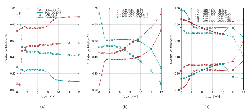
Figure 1: Contributions from single (red) and double (turquoise) excitations in the first ${}^{1}\Sigma_{g}^{+}$ excited state of Yb₂ from different quantum chemistry methods: (a) EOM-CCSD and CAS(4,8)SCF, (b) EOM-pCCD-CCS (with and without orbital optimization), and (c) EOM-pCCD-LCCSD (with and without orbital optimization and different point group symmetries). Results for EOM-pCCD+S are similar to EOM-pCCD-CCS and are thus not shown in the Figure. For CAS(4,8)SCF, the individual contributions are determined from the weights of all active space configurations with coefficients larger than 0.05 only.

Reference spin–orbit electronic spectrum

The reference spin-orbit Yb₂ excited-state potential energy surfaces are presented in Figure 2. If spin-orbit coupling is accounted for, the minima of each excited potential energy curve are shifted towards shorter inter-atomic distances. Furthermore, the whole spectrum is rather dense, especially all states approaching the atomic limits ¹S+³P₀, ¹S+³P₁, and ¹S+³P₂ lie very close to each other. Higher lying are the $1_{u}(^{1}\Pi_{u})$ and $0_{g}^{+}(^{1}\Sigma_{g}^{+})$ states that dissociate into the ¹S+¹P₁ atomic limit. A distinct feature of the Yb₂ electronic spectrum is the presence of 0${}_{g}^{+}$ excited states originating from the repulsive (spin–free) ${}^{3}\Sigma_{g}^{+}$ state with a specific shape of the potential energy surface compared to the remaining excited states.

The SO-CAS(4,8)PT2 spectroscopic parameters for the excited states in Yb₂ are collected in Tables 8–11. For convenience, the spectroscopic characteristics of all investigated excited states are grouped into four blocks according to their atomic dissociation limit, Table 8 for the ¹S+³P₀, Table 9 for the ¹S+³P₁, Table 10 for the ¹S+³P₂, and Table 11 for the ¹S+¹P₁ atomic limits, respectively. In the lowest-lying part of the spectrum, our TZ-ANO-RCC results qualitatively match the ECP/SO-MRCI spectroscopic parameters determined by Wang and Dolg ³⁶. The differences increase, however, when larger basis sets are used within the SO-CAS(4,8)PT2 approach. This observation suggests the need for large basis set sizes when targeting excited states in the Yb₂ dimer. In general, the size of the atomic basis set affects all spectroscopic parameters. A large basis set considerably shortens the optimal bond lengths, lowers the adiabatic excitation energies, and increases potential energy depths. Harmonic vibrational frequencies are only slightly altered by the choice of the basis set.

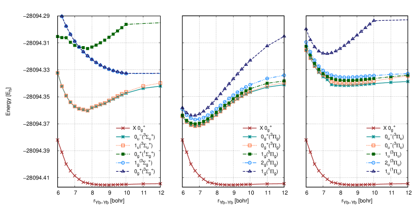
Figure 2: SO-CAS(4,8)PT2 electronic spectrum of Yb₂ using the large-ANO-RCC basis set. The whole spectrum is divided into contributions from $\Sigma$, $\Pi_{u}$, and $\Pi_{g}$ states (from left to right).

State	basis	$\mathrm{r_{e}[a_{0}]}$	$\mathrm{\omega_{e}[cm^{-1}]}$	$\mathrm{D_{e}[cm^{-1}]}$	$\mathrm{T_{e}[cm^{-1}]}$
0${}_{g}^{-}$(${}^{3}\Pi_{g}$$)$	TZ-ANO-RCC	6.938	69	5 627	10 589
	QZ-ANO-RCC	6.874	70	6 038	10 294
	large-ANO-RCC	6.778	73	6 968	9 561
	ECP(MRCI) 36	6.969	65	4 759	13 147
0${}_{u}^{-}$(${}^{3}\Sigma_{u}^{+}$$)$	TZ-ANO-RCC	7.693	54	3 132	13 084
	QZ-ANO-RCC	7.640	56	3 506	12 826
	large-ANO-RCC	7.568	60	4 332	12 197
	ECP(MRCI) 36	7.544	54	2 662	15 244

Table 8: SO-CAS(4,8)PT2 adiabatic electronic states of Yb2 dissociating into the ¹S+³P₀ atomic limit. $\mathrm{r_{e}}$ denotes the equilibrium bond length, $\mathrm{\omega_{e}}$ the vibrational frequency, $\mathrm{D_{e}}$ the potential depth, and $\mathrm{T_{e}}$ the adiabatic excitation energy, respectively.

State	basis	$\mathrm{r_{e}[a_{0}]}$	$\mathrm{\omega_{e}[cm^{-1}]}$	$\mathrm{D_{e}[cm^{-1}]}$	$\mathrm{T_{e}[cm^{-1}]}$
0${}_{g}^{+}(^{3}\Pi_{g})$	TZ-ANO-RCC	6.939	69	6 173	10 600
	QZ-ANO-RCC	6.877	70	6 584	10 303
	large-ANO-RCC	6.784	73	7 508	9 578
	ECP(MRCI) 36	6.971	66	5 404	13 147
1${}_{g}(^{3}\Pi_{g})$	TZ-ANO-RCC	6.920	69	5 775	10 998
	QZ-ANO-RCC	6.877	70	6 584	10 303
	large-ANO-RCC	6.753	72	7 154	9 933
	ECP(MRCI) 36	6.984	65	4 839	13 711
1${}_{u}(^{3}\Sigma_{u}^{+})$	TZ-ANO-RCC	7.681	55	3 618	13 155
	QZ-ANO-RCC	7.633	57	3 998	12 889
	large-ANO-RCC	7.566	61	4 837	12 249
	ECP(MRCI) 36	7.544	54	2 662	15 244
0${}_{u}^{+}(^{3}\Pi_{u})$	TZ-ANO-RCC	8.927	17	500	16 272
	QZ-ANO-RCC	8.575	25	652	16 236
	large-ANO-RCC	8.450	32	977	16 109
	ECP(MRCI) 36	8.714	26	484	18 067

Table 9: SO-CAS(4,8)PT2 adiabatic electronic states of Yb2 dissociating into the ¹S+³P₁ atomic limit. $\mathrm{r_{e}}$ denotes the equilibrium bond length, $\mathrm{\omega_{e}}$ the vibrational frequency, $\mathrm{D_{e}}$ the potential depth, and $\mathrm{T_{e}}$ the adiabatic excitation energy, respectively.

State	basis	$\mathrm{r_{e}[a_{0}]}$	$\mathrm{\omega_{e}[cm^{-1}]}$	$\mathrm{D_{e}[cm^{-1}]}$	$\mathrm{T_{e}[cm^{-1}]}$
2${}_{g}(^{3}\Pi_{g})$	TZ-ANO-RCC	6.964	69	6 303	11 651
	QZ-ANO-RCC	6.909	70	6 685	11 354
	large-ANO-RCC	6.814	72	7 605	10 632
	ECP(MRCI) 36	6.998	66	5 565	14 437
0${}_{u}^{-}(^{3}\Pi_{u})$	TZ-ANO-RCC	8.626	29	1 403	16 552
	QZ-ANO-RCC	8.528	32	1 549	16 490
	large-ANO-RCC	8.490	32	1 786	16 450
	ECP(MRCI) 36	8.404	31	1 452	18 551
1${}_{u}(^{3}\Pi_{u})$	TZ-ANO-RCC	8.820	23	902	17 052
	QZ-ANO-RCC	8.668	24	1 012	17 026
	large-ANO-RCC	8.368	30	1 284	16 952
	ECP(MRCI) 36	8.596	27	1 049	18 954
2${}_{u}(^{3}\Pi_{u})$	TZ-ANO-RCC	8.931	19	382	17 572
	QZ-ANO-RCC	8.716	21	486	17 552
	large-ANO-RCC	8.342	29	755	17 482
	ECP(MRCI) 36	8.755	27	484	19 519
1${}_{g}(^{1}\Pi_{g},^{3}\Sigma_{g}^{+})$	TZ-ANO-RCC	12.533	26	88	17 866
	QZ-ANO-RCC	11.160	18	81	17 957
	large-ANO-RCC	10.943	21	321	17 916
	ECP(MRCI) 36	6.837	76	1 129	18 873

Table 10: SO-CAS(4,8)PT2 adiabatic electronic states of Yb2 dissociating into the ¹S+³P₂ atomic limit. $\mathrm{r_{e}}$ denotes the equilibrium bond length, $\mathrm{\omega_{e}}$ the vibrational frequency, $\mathrm{D_{e}}$ the potential depth, and $\mathrm{T_{e}}$ the adiabatic excitation energy, respectively.

State	basis	$\mathrm{r_{e}[a_{0}]}$	$\mathrm{\omega_{e}[cm^{-1}]}$	$\mathrm{D_{e}[cm^{-1}]}$	$\mathrm{T_{e}[cm^{-1}]}$
0${}_{u}^{+}(^{1}\Sigma_{u}^{+})$	TZ-ANO-RCC	7.173	81	9 089	19 194
	QZ-ANO-RCC	7.378	55	8 765	18 947
	large-ANO-RCCa	-	-	-	-
	ECP(MRCI) 36	7.347	59	7 743	23 713
1${}_{u}(^{1}\Pi_{u})$	TZ-ANO-RCC	7.312	66	5 582	22 702
	QZ-ANO-RCC	7.272	67	5 484	22 228
	large-ANO-RCC	7.199	69	6 127	21 328
	ECP(MRCI) 36	7.170	68	5 001	26 455
0${}_{g}^{+}(^{1}\Sigma_{g}^{+})$	TZ-ANO-RCC	7.505	65	5 041	23 243
	QZ-ANO-RCC	7.524	57	4 853	22 859
	large-ANO-RCC	7.666	55	5 011	22 444
	ECP(MRCI) 36	7.514	51	3 549	27 907
1${}_{g}(^{3}\Sigma_{g}^{+},^{1}\Pi_{g})$	TZ-ANO-RCC	7.852	60	1 917	26 366
	QZ-ANO-RCC	7.802	64	2 200	25 512
	large-ANO-RCC	7.704	69	3 032	24 423
	ECP(MRCI) 36	8.484	115	9 033	22 422

Table 11: SO-CAS(4,8)PT2 adiabatic electronic states of Yb2 dissociating into the ¹S+¹P₁ atomic limit. $\mathrm{r_{e}}$ denotes the equilibrium bond length, $\mathrm{\omega_{e}}$ the vibrational frequency, $\mathrm{D_{e}}$ the potential depth, and $\mathrm{T_{e}}$ the adiabatic excitation energy, respectively.

• ^a not computed due to technical difficulties

CONCLUSIONS AND OUTLOOK

In this work, we have investigated the electronic structure of atomic and molecular ytterbium using modern, state-of-the-art quantum chemistry methods. Our numerical analysis suggests that SO-CASPT2 with inclusion of the 5d orbitals into the active space can accurately reproduce the experimental energy levels of Yb. The singlet excited states in the Yb atom can be reliably modeled within the EOM-CCSD approach. A similar accuracy in excited state energies and properties can also be obtained with simplified alternatives, such as EOM-pCCD-LCCSD.

Furthermore, we report a new set of spectroscopic parameters for the ground-state potential energy curve of the Yb₂ dimer. Our best estimate based on CCSD(T) reference calculations with an uncontracted ANO-RCC basis set gives an optimal bond length of $\mathrm{r_{e}}=8.814$ bohr, a harmonic vibrational frequencies of $\omega_{e}=21$ cm^-1, and a potential energy depth of $\mathrm{D_{e}}=579$ cm^-1 and can be considered as the limit of present-day quantum chemistry calculations. The CCSD potential energy curve, which results in an elongated bond length and underestimated potential energy depth compared to CCSD(T), can be reliably approximated using the pCCD-LCSSD and CAS(4,8)PT2 approaches.

The quantum chemical modeling of excited states in the Yb₂ dimer remains, however, a remarkable challenge for present-day quantum chemistry. First, it is technically challenging to include d-type and f-type orbitals in molecular CASSCF calculations, limiting the manifold of electronic excitations to electron transfer form 6s to 6p atomic orbitals. Second, the ${}^{1}\Sigma_{g}^{+}$ excited state has a double excitation character that is difficult to describe using conventional coupled cluster type methods such as EOM-CCSD. The EOM-pCCD-LCCSD approach is advantageous here as it provides accurate spectroscopic constants, yet being able to correctly model the doubly excited ${}^{1}\Sigma^{+}$ potential energy curve. Most importantly, our numerical results indicate that the simplified EOM-pCCD-LCCSD formalism poses an alternative to the conventional EOM-CCSD approach to model excited states. Specifically, for most excited states, EOM-pCCD-LCCSD (with or without orbital optimization) provides spectroscopic constants that deviate less from the SO-CAS(4,8)PT2 reference values. This is especially advantageous for excited states with significant bi-excited character, where EOM-CCSD is known to fail.

Finally, we report a new set of reference spectroscopic constants for the low-lying excited states of the Yb₂ dimer using the SO-CAS(4,8)PT2 approach. Our data is a significant improvement over the existing ECP/SO-MRCI results of Wang and Dolg ³⁶ as they include an all-electron basis set and a more rigorous treatment of scalar relativistic and electron correlation effects within the CASPT2 approach. Moreover, we investigate the convergence of the spectroscopic parameters (optimal bond lengths, vibrational frequencies, potential energy depths, and adiabatic excitation energies) with respect to the size of the basis set, which highlights the need for large basis set when modeling excited state potential energy curves in Yb₂. We would like to stress that new quantum chemistry methods are desirable that can be used to reliably model the complete set of excited state potential energy curves in challenging molecules like the Yb₂ dimer.

High quality potential curves for the Yb₂ molecule are critical for future investigations in the fields of cold atomic collisions and ultracold molecules, including an improved description of the strengths and widths of intercombination line optical Feshbach resonances, ^{12, 86} searching for routes to Yb₂ rovibrational ground state, ⁸⁷ or calculating the sensitivity of deeply bound molecular clock states to the variation of the proton-to-electron mass ratio ^{30, 21}. Finally, these potential curves provide a valuable starting point for laser-induced fluorescence spectroscopy spectroscopy of ytterbium molecules.

ACKNOWLEDGMENTS

P.T. thanks a POLONEZ 1 research grant (no. 2015/19/P/ST4/02480) financed by Marie-Skłodowska-Curie COFUND. This project has received funding from the European Union’s Horizon 2020 research and innovation programme under the Marie Skłodowska-Curie grant agreement No 665778. K.B. acknowledges financial support from a Marie-Skłodowska-Curie Individual Fellowship project no. 702635–PCCDX and a scholarship for outstanding young scientists from the Ministry of Science and Higher Education. M.B. and P.Sz.Ż. acknowledge financial support from the National Science Centre, Poland (no. 2017/25/B/ST4/01486). The research is part of an ongoing research program of the National Laboratory FAMO in Torun, Poland. D.K. acknowledges support from an OPUS grant of the National Science Centre, Poland (no. DEC-2012/07/B/ST4/01347) and COST Action CM1405 “Molecules in Motion” (MOLIM).

Calculations have been carried out using resources provided by Wroclaw Centre for Networking and Supercomputing (http://wcss.pl), grant nos. 353, 411, and 412.

References

- Honda et al. 2002 K. Honda, Y. Takasu, T. Kuwamoto, M. Kumakura, Y. Takahashi, and T. Yabuzaki, Phys. Rev. A 66, 021401 (2002).
- Kitagawa et al. 2008 M. Kitagawa, K. Enomoto, K. Kasa, Y. Takahashi, R. Ciuryło, P. Naidon, and P. S. Julienne, Phys. Rev. A 77, 012719 (2008).
- Takasu et al. 2003 Y. Takasu, K. Maki, K. Komori, T. Takano, K. Honda, M. Kumakura, T. Yabuzaki, and Y. Takahashi, Phys. Rev. Lett. 91, 040404 (2003).
- Fukuhara et al. 2007 T. Fukuhara, S. Sugawa, and Y. Takahashi, Phys. Rev. A 76, 051604(R) (2007).
- Fukuhara et al. 2009 T. Fukuhara, S. Sugawa, Y. Takasu, and Y. Takahashi, Phys. Rev. A 79, 021601(R) (2009).
- Sugawa et al. 2011 S. Sugawa, R. Yamazaki, S. Taie, and Y. Takahashi, Phys. Rev. A 84, 011610(R) (2011).
- Ludlow et al. 2015 A. D. Ludlow, M. M. Boyd, J. Ye, E. Peik, and P. O. Schmidt, Rev. Mod. Phys. 87, 638 (2015).
- McGrew et al. 2018 W. F. McGrew, X. Zhang, R. J. Fasano, S. A. Schäffer, K. Beloy, D. Nicolodi, R. C. Brown, N. Hinkley, G. Milani, M. Schioppo, et al., Nature 564, 87 (2018).
- Livi et al. 2016 L. F. Livi, G. Cappellini, M. Diem, L. Franchi, C. Clivati, M. Frittelli, F. Levi, D. Calonico, J. Catani, M. Inguscio, et al., Phys. Rev. Lett. 117, 1 (2016).
- Jones et al. 2006 K. M. Jones, E. Tiesinga, P. D. Lett, and P. S. Julienne, Rev. Mod. Phys. 78, 483 (2006).
- Tojo et al. 2006 S. Tojo, M. Kitagawa, K. Enomoto, Y. Kato, Y. Takasu, M. Kumakura, and Y. Takahashi, Phys. Rev. Lett. 96, 153201 (2006).
- Borkowski et al. 2009 M. Borkowski, R. Ciuryło, P. S. Julienne, S. Tojo, K. Enomoto, and Y. Takahashi, Phys. Rev. A 80, 012715 (2009).
- Borkowski et al. 2017 M. Borkowski, A. A. Buchachenko, R. Ciuryło, P. S. Julienne, H. Yamada, Y. Kikuchi, K. Takahashi, Y. Takasu, and Y. Takahashi, Phys. Rev. A 96, 063405 (2017).
- Takasu et al. 2012 Y. Takasu, Y. Saito, Y. Takahashi, M. Borkowski, R. Ciuryło, and P. S. Julienne, Phys. Rev. Lett. 108, 173002 (2012).
- Enomoto et al. 2008a K. Enomoto, M. Kitagawa, S. Tojo, and Y. Takahashi, Phys. Rev. Lett. 100, 123001 (2008a).
- Ciuryło et al. 2005 R. Ciuryło, E. Tiesinga, and P. S. Julienne, Phys. Rev. A 71, 030701(R) (2005).
- Enomoto et al. 2008b K. Enomoto, K. Kasa, M. Kitagawa, and Y. Takahashi, Phys. Rev. Lett. 101, 203201 (2008b).
- Kim et al. 2016 M.-S. Kim, J. Lee, J. H. Lee, Y. Shin, and J. Mun, Phys. Rev. A 94, 042703 (2016).
- Franchi et al. 2017 L. Franchi, L. F. Livi, G. Cappellini, G. Binella, M. Inguscio, J. Catani, and L. Fallani, New J. Phys 19, 103037 (2017).
- Bouganne et al. 2017 R. Bouganne, M. B. Aguilera, A. Dareau, E. Soave, J. Beugnon, and F. Gerbier, New J. Phys. 19, 113006 (2017).
- Borkowski 2018 M. Borkowski, Phys. Rev. Lett. 120, 083202 (2018).
- Pagano et al. 2015 G. Pagano, M. Mancini, G. Cappellini, L. Livi, C. Sias, J. Catani, M. Inguscio, and L. Fallani, Phys. Rev. Lett. 115 (2015).
- Cappellini et al. 2019 G. Cappellini, L. F. Livi, L. Franchi, D. Tusi, D. Benedicto Orenes, M. Inguscio, J. Catani, and L. Fallani, Phys. Rev. X 9, 011028 (2019).
- Kato et al. 2013 S. Kato, S. Sugawa, K. Shibata, R. Yamamoto, and Y. Takahashi, Phys. Rev. Lett. 110, 173201 (2013).
- Takasu et al. 2017 Y. Takasu, Y. Fukushima, Y. Nakamura, and Y. Takahashi, Phys. Rev. A 96, 023602 (2017).
- Green et al. 2016 D. G. Green, C. L. Vaillant, M. D. Frye, M. Morita, and J. M. Hutson, Phys. Rev. A 93, 022703 (2016).
- Safronova et al. 2018 M. S. Safronova, S. G. Porsev, C. Sanner, and J. Ye, Phys. Rev. Lett. 120, 173001 (2018).
- Meyer and Bohn 2009 E. R. Meyer and J. L. Bohn, Phys. Rev. A 80, 042508 (2009).
- Borkowski et al. 2018 M. Borkowski, A. A. Buchachenko, R. Ciuryło, P. S. Julienne, H. Yamada, Y. Kikuchi, Y. Takasu, and Y. Takahashi (2018), 1612.03842, URL http://arxiv.org/abs/1612.03842.
- Zelevinsky et al. 2008 T. Zelevinsky, S. Kotochigova, and J. Ye, Phys. Rev. Lett. 100, 043201 (2008).
- Takekoshi et al. 2014 T. Takekoshi, L. Reichsöllner, A. Schindewolf, J. M. Hutson, C. R. Le Sueur, O. Dulieu, F. Ferlaino, R. Grimm, and H. C. Nägerl, Phys. Rev. Lett. 113, 1 (2014).
- Fleig 2011 T. Fleig, Chem. Phys. 395, 2 (2011).
- Buchachenko et al. 2007 A. A. Buchachenko, G. Chałasiński, and M. M. Szczęśniak, Eur. Phys. J. D 45, 147 (2007).
- Safronova et al. 2012 M. S. Safronova, S. G. Porsev, and C. W. Clark, Phys. Rev. Lett. 109, 230802 (2012).
- Porsev et al. 2014 S. G. Porsev, M. S. Safronova, A. Derevianko, and C. W. Clark, Phys. Rev. A 89, 012711 (2014).
- Wang and Dolg 1998 Y. Wang and M. Dolg, Theor. Chem. Acc. 100, 124 (1998).
- Roos et al. 2008 B. O. Roos, R. Lindh, P.-A. Malmqvist, V. Veryazov, P.-O. Widmark, and A. C. Borin, J. Phys. Chem. A 112, 11431 (2008).
- Douglas and Kroll 1974 N. Douglas and N. M. Kroll, Ann. Phys. 82, 89 (1974).
- Hess 1986 B. A. Hess, Phys. Rev. A 33, 3742 (1986).
- Johnson et al. 2013 P. A. Johnson, P. W. Ayers, P. A. Limacher, S. de Baerdemacker, D. van Neck, and P. Bultinck, J. Chem. Theor. Comput. 1003, 101 (2013).
- Stein et al. 2014 T. Stein, T. M. Henderson, and G. E. Scuseria, J. Chem. Phys. 140, 214113 (2014).
- 42 PIERNIK, a pythonic ab initio electronic structure program, (2019), written by F. Brzęk, A. Leszczyk, A. Nowak, K. Boguslawski, D. Kędziera, P. Tecmer, and P. S. Żuchowski.
- Boguslawski et al. 2014a K. Boguslawski, P. Tecmer, P. W. Ayers, P. Bultinck, S. De Baerdemacker, and D. Van Neck, Phys. Rev. B 89, 201106(R) (2014a).
- Boguslawski et al. 2014b K. Boguslawski, P. Tecmer, P. A. Limacher, P. A. Johnson, P. W. Ayers, P. Bultinck, S. De Baerdemacker, and D. Van Neck, J. Chem. Phys. 140, 214114 (2014b).
- Boguslawski et al. 2014c K. Boguslawski, P. Tecmer, P. W. Ayers, P. Bultinck, S. De Baerdemacker, and D. Van Neck, J. Chem. Theory Comput. 10, 4873 (2014c).
- Boguslawski and Ayers 2015 K. Boguslawski and P. W. Ayers, J. Chem. Theory Comput. 11, 5252 (2015).
- Boguslawski 2016 K. Boguslawski, J. Chem. Phys. 145, 234105 (2016).
- Boguslawski 2017 K. Boguslawski, J. Chem. Phys. 147, 139901 (2017).
- Boguslawski 2019 K. Boguslawski, J. Chem. Theory Comput. 15, 18 (2019).
- Leszczyk et al. 2019 A. Leszczyk, P. Tecmer, and K. Boguslawski, in Transition Metals in Coordination Environments, Challenges and Advances in Computational Chemistry and Physics (Springer, Cham (Switzerland), 2019), vol. 29, chap. New Strategies in Modeling Electronic Structures and Properties with Applications to Actinides, pp. 121–160.
- Deegan and Knowles 1994 M. J. O. Deegan and P. J. Knowles, Chem. Phys. Lett. 227, 321 (1994).
- Korona and Werner 2003 T. Korona and H.-J. Werner, J. Chem. Phys. 118, 3006 (2003).
- Werner et al. 2012a H. Werner, P. J. Knowles, G. Knizia, F. R. Manby, M. Schütz, and et al., Molpro, version 2012.1, a package of ab initio programs (2012a), see http://www.molpro.net.
- Werner et al. 2012b H. Werner, P. J. Knowles, G. Knizia, F. R. Manby, and M. Schütz, WIREs Comput. Mol. Sci. 2, 242 (2012b).
- Werner and Knowles 1985 H. Werner and P. J. Knowles, J. Chem. Phys. 82, 5053 (1985).
- Werner and Knowles 1988 H. Werner and P. J. Knowles, J. Chem. Phys. 89, 5803 (1988).
- Roos et al. 1980 B. O. Roos, P. R. Taylor, and P. E. M. Siegbahn, Chem. Phys. 48, 157 (1980).
- Siegbahn et al. 1981 P. E. M. Siegbahn, J. Almlöf, A. Heiberg, and B. O. Roos, J. Chem. Phys. 74, 2384 (1981).
- Andersson et al. 1990 K. Andersson, P.-Å. Malmqvist, B. O. Roos, A. J. Sadlej, and K. Woliński, J. Phys. Chem. 94, 5483 (1990).
- Andersson et al. 1992 K. Andersson, P.-Å. Malmqvist, and B. O. Roos, J. Chem. Phys. 96, 1218 (1992).
- Finley et al. 1998 J. Finley, P.-Å. Malmqvist, B. O. Roos, and L. Serrano-Andrés, Chem. Phys. Lett. 288, 299 (1998).
- G. Karlström, R. Lindh, P.-Å. Malmqvist, B. O. Roos, U. Ryde, V. Veryazov, P.-O. Widmark, M. Cossi, B. Schimmelpfennig, P. Neogrády and L. Seijo 2003 G. Karlström, R. Lindh, P.-Å. Malmqvist, B. O. Roos, U. Ryde, V. Veryazov, P.-O. Widmark, M. Cossi, B. Schimmelpfennig, P. Neogrády and L. Seijo, Comput. Mater. Sci. 28, 222 (2003).
- F. Aquilante, L. De Vico, N. Ferré, G. Ghigo, P.-Å. Malmqvist, P. Neogrády, T. B. Pedersen, M. Pitonak, M. Reiher, B. O. Roos, L. Serrano-Andrés, M. Urban, V. Veryazov and R. Lindh 2010 F. Aquilante, L. De Vico, N. Ferré, G. Ghigo, P.-Å. Malmqvist, P. Neogrády, T. B. Pedersen, M. Pitonak, M. Reiher, B. O. Roos, L. Serrano-Andrés, M. Urban, V. Veryazov and R. Lindh, J. Comput. Chem. 31, 224 (2010).
- V. Veryazov, P.-O. Widmark, L. Serrano-Andrés, R. Lindh and B. O. Roos 2004 V. Veryazov, P.-O. Widmark, L. Serrano-Andrés, R. Lindh and B. O. Roos, Int. J. Quantum Chem. 100, 626 (2004).
- F. Aquilante, J. Autschbach, R. K. Carlson, L. F. Chibotaru, M. G. Delcey, L. De Vico, I. Fdez. Galván, N. Ferré, L. M. Frutos, L. Gagliardi, M. Garavelli, A. Giussani, C. E. Hoyer et al. 2016 F. Aquilante, J. Autschbach, R. K. Carlson, L. F. Chibotaru, M. G. Delcey, L. De Vico, I. Fdez. Galván, N. Ferré, L. M. Frutos, L. Gagliardi, M. Garavelli, A. Giussani, C. E. Hoyer et al., J. Comput. Chem. 37, 506 (2016).
- Ghigo et al. 2004 G. Ghigo, B. O. Roos, and P.-Å. Malmqvist, Chem. Phys. Lett. 396, 142 (2004).
- Hess et al. 1996 B. A. Hess, C. M. Marian, U. Wahlgren, and O. Gropen, Chem. Phys. Lett. 251, 365 (1996).
- Marian and Wahlgren 1996 C. M. Marian and U. Wahlgren, Chem. Phys. Lett. 251, 357 (1996).
- Schimmelpfennig et al. 1998 B. Schimmelpfennig, L. Maron, U. Wahlgren, C. Teichteil, H. Fagerli, and O. Gropen, Chem. Phys. Lett. 286, 267 (1998).
- Malmqvist et al. 2002 P.-Å. Malmqvist, B. O. Roos, and B. Schimmelpfennig, Chem. Phys. Lett. 357, 230 (2002).
- Abramowitz and Stegun 1970 M. Abramowitz and I. A. Stegun, Handbook Of Mathematical Functions With Formulas, Graphs, And Mathematical Tables (Dover, New York, 1970).
- Sansonetti and Martin 2005 J. E. Sansonetti and W. C. Martin, J. Phys. Chem. Ref. Data 34, 1559 (2005).
- Meggers and Tech 1978 W. F. Meggers and J. L. Tech, J. Res. Natl. Bur. Stand. U.S. 83, 13 (1978).
- Mies et al. 1978 F. Mies, W. Stevens, and M. Krauss, J. Mol. Spectrosc. 72, 303 (1978).
- Roos 2008 B. O. Roos, in Radiation Induced Molecular Phenomena in Nucleic Acids (Springer, 2008), pp. 125–156.
- Suzer and Andrews 1988 S. Suzer and L. Andrews, J. Chem. Phys. 89, 5514 (1988).
- Wang et al. 1999 Y. Wang, F. Schautz, H.-J. Flad, and M. Dolg, J. Phys. Chem. A 103, 5091 (1999).
- Řezáč and Hobza 2013 J. Řezáč and P. Hobza, J. Chem. Theory Comput. 9, 2151 (2013).
- Boys and Bernardi 1970 S. Boys and F. Bernardi, Mol. Phys. 19, 553 (1970).
- Goodfriend 1984 P. Goodfriend, Spectrochim. Acta A: Mol. Spectr. 40, 283 (1984).
- Lee and Taylor 1989 T. J. Lee and P. R. Taylor, Int. J. Quantum Chem. 23, 199 (1989).
- Mosyagin et al. 2009 N. S. Mosyagin, P. A. N., and A. Titov, pp. 1–10 (2009), 0901.0077v6.
- Boguslawski et al. 2014d K. Boguslawski, P. Tecmer, P. A. Limacher, P. A. Johnson, P. W. Ayers, P. Bultinck, S. de Baerdemacker, and D. van Neck, J. Chem. Phys. 140, 214114 (2014d).
- Boguslawski et al. 2014e K. Boguslawski, P. Tecmer, P. A. Limacher, P. A. Johnson, P. W. Ayers, P. Bultinck, S. de Baerdemacker, and D. van Neck, J. Chem. Theory Comput. 10, 4873 (2014e).
- Helgaker et al. 1997 T. Helgaker, W. Klopper, H. Koch, and J. Noga, J. Chem. Phys. 106, 9639 (1997).
- Nicholson et al. 2015 T. L. Nicholson, S. Blatt, B. J. Bloom, J. R. Williams, J. W. Thomsen, J. Ye, and P. S. Julienne, Phys. Rev. A 92, 022709 (2015).
- Sage et al. 2005 J. M. Sage, S. Sainis, T. Bergeman, and D. DeMille, Phys. Rev. Lett. 94, 203001 (2005).