Coherent spin transport through helical edge states of topological insulator

Abstract

We study coherent spin transport through helical edge states of topological insulator tunnel-coupled to metallic leads. We demonstrate that unpolarized incoming electron beam acquires finite polarization after transmission through such a setup provided that edges contain at least one magnetic impurity. The finite polarization appears even in the fully classical regime and is therefore robust to dephasing. There is also a quantum magnetic field-tunable contribution to the polarization, which shows sharp identical Aharonov-Bohm resonances as a function of magnetic flux—with the period $hc/2e$—and survives at relatively high temperature. We demonstrate that this tunneling interferometer can be described in terms of ensemble of flux-tunable qubits giving equal contributions to conductance and spin polarization. The number of active qubits participating in the charge and spin transport is given by the ratio of the temperature and the level spacing. The interferometer can effectively operate at high temperature and can be used for quantum calculations. In particular, the ensemble of qubits can be described by a single Hadamard operator. The obtained results open wide avenue for applications in the area of quantum computing.

I Introduction

Quantum information processing attracts enormous interest of a broad scientific community National Academies of Sciences et al. (2019). Although the promise of quantum computers was recognized about thirty years ago, the real breakthrough in creation of their key elements — networks of coherent spin qubits — was achieved only in the last decade Zwanenburg et al. (2013). The principal obstacle for further progress is connected with fast spin relaxation and dephasing, which prevent creation of spin polarization and coherent spin transmission over long distances. Another challenging yet unsolved task of primary importance for information processing and quantum networking is all-electrical control of the electron spins Wolf et al. (2001); Žutić et al. (2004); Awschalom and Flatté (2007).

An effective low-cost room-temperature solution of these problems would allow for tunable coherent transmission of the spin polarization over long distances. Ever since the proposal of spin field effect transistor (SpinFET) Datta and Das (1990), numerous attempts to achieve coherent spin transmission and all-electrical manipulation by using setups of various design were unsuccessful Crooker et al. (2005); Appelbaum et al. (2007); Lou et al. (2007); Koo et al. (2009); Kum et al. (2012); Wunderlich et al. (2010); Betthausen et al. (2012). In semiconductor devices spin polarization usually originates from spin-orbit coupling and is never sufficiently large, in particular due to low efficiency of the spin injection Schmidt et al. (2000). It can be somewhat increased by using non-electrical elements such as ferromagnetic contacts, which however dramatically deteriorate transport properties of the system. Furthermore, injected polarization rapidly decays due to spin relaxation processes.

In this Letter, we propose essential steps towards solving several critical problems of quantum information processing: spin filtering, long-distance spin transfer, and effective spin manipulation. Physically, spin filter blocks transmission of particles with one spin orientation, say spin-down, so that outgoing current acquires spin-up polarization. We introduce a method for creation of spin-polarized electron beams based on using of helical edge states (HES) of two-dimensional (2D) topological insulator. Spin transport in HES was already discussed at zero temperature (see Refs. An et al. (2012a, b); Michetti and Recher (2011); Battilomo et al. (2018); Zare (2019) and references therein). Here, we demonstrate that, remarkably, the finite spin polarization arises at high temperature, even in the fully classical regime and is therefore robust to dephasing.

The suggested method allows for 100% spin polarization and therefore has essential advantages over the existing approaches to spin filtering and spin transfer based on resonant tunneling diodes Wójcik et al. (2012); Slobodskyy et al. (2003), quantum dots Hauptmann et al. (2008); Folk et al. (2003), Y junctions Wójcik et al. (2015); Matityahu et al. (2017), and Aharonov-Bohm (AB) interferometers based on conventional materials Shmakov et al. (2012). In all these structures spin polarization achieved so far was sufficiently small. More promising candidates for spin filtering are the quantum point contacts (QPC) with strong SO interaction and engineered structures incorporating QPC as building blocks Tsai et al. (2013); Debray et al. (2009); Das et al. (2012); Bhandari et al. (2013); Kohda et al. (2012); Chuang et al. (2015). Although the predicted spin polarization in QPC-based structures operating in the single-mode regime of SpinFET can be quite high Bhandari et al. (2013), one of the main problems in the way of coherent spin control—fast spin relaxation—remains unresolved. This implies that spin polarization cannot be transferred over a distance exceeding the spin relaxation length which is typically not quite large for conventional semiconductors with SO interaction.

Here, we study spin transport through the edge states of topological insulator and show that the spin polarization can be transferred for large distances on the order of the edge state’s length. This distance can be made even longer by building arrays of several HES. In contrast to all previous studies of spin-selective transport via HES, we find that large spin polarization can be created and transferred at high temperatures thus opening a wide avenue for application in quantum computing. In particular, we demonstrate that obtained results can be formulated in terms of flux-tunable ensemble of qubits giving equal contribution to charge and spin transport. Our study is a direct generalization of recent research on controlling quantum qubits by various types of interferometers and using them for quantum computing Földi et al. (2005); Michetti and Recher (2011); Chen et al. (2014); Bautze et al. (2014); Bäuerle et al. (2018); Bordone et al. (2019); Bellentani et al. (2020). In particular, it was predicted that conventional interferometers with spin-orbit (SO) interaction (or an array of such interferometers) can be used as one-qubit quantum gates of various types (X-gate, Z-gate, phase gate, and Hadamard gate) Földi et al. (2005). Such qubits can be controlled by changing the magnetic field and the strength of the SO interaction Földi et al. (2005); Michetti and Recher (2011). Taking into account the electron-electron interaction makes it also possible to construct effective two-qubit computational schemes in two coupled interferometers based on conventional materials Bautze et al. (2014); Bäuerle et al. (2018), on edge states of the integer quantum Hall effect Bordone et al. (2019); Bellentani et al. (2020) and on helical states Chen et al. (2014). Signatures of electron-electron interaction in HES was already observed experimentally Stühler et al. (2020); Strunz et al. (2020).

The computational schemes, proposed so far, imply the control of so-called flying qubits with a given energy and can be directly applied at zero temperature. However, in realistic systems, the electrons enter the interferometer from thermalized contacts, which implies averaging within the temperature window around the Fermi energy. Since the phases accumulated by an electron passing through two arms of the interferometer are energy dependent, the question arises whether thermal averaging violates the efficiency of the proposed computational schemes. This is exactly the question that we address in this work. We demonstrate that using tunneling interferometers based on helical edge states allows one for transfer of spin polarization at large distance as well as quantum computing at high temperatures. We also find that the energy levels of almost closed interferometer form an ensemble of $T/\Delta$ qubits providing equal contributions into the spin and charge transport. This means that in HES based setups the interference survives thermal averaging com (a). Hence, using of such interferometers might be a neat way to overcome the main problems of spin-networking, namely, sensitivity of spin polarization to dephasing and relaxation processes and the requirement of very low temperature.

II Results

II.1 Key idea

We propose to explore unique properties of HES existing at the edges of 2D topological insulators, which are materials insulating in the bulk, but exhibiting conducting channels at the surface or at the boundaries. In particular, the 2D topological insulator phase was predicted in HgTe quantum wells Kane and Mele (2005); Bernevig et al. (2006) and confirmed by direct measurements of conductance of the edge states König et al. (2007) and by the experimental analysis of the non-local transport Roth et al. (2009); Gusev et al. (2011); Brüne et al. (2012); Kononov et al. (2015). These states are one-dimensional helical channels where the electron spin projection is connected with its velocity, e.g. electrons traveling in one direction are characterized by spin “up”, while electrons moving in the opposite direction are characterized by spin “down”. Remarkably, the electron transport via HES is ideal, in the sense that electrons do not experience backscattering from conventional non-magnetic impurities, similarly to what occurs in edge states of Quantum Hall Effect systems, but without invoking high magnetic fields (for detailed discussion of properties of HES see Refs. Hasan and Kane (2010); Qi and Zhang (2011)).

Hence, in the absence of magnetic disorder, the boundary states are ballistic and topologically protected from external perturbations. Due to this key advantage a spin traveling along the edge does not relax, so that such states perfectly match the purposes of quantum spin networking. Importantly, even a non-magnetic lead splits the incoming electron beam into two parts: right-moving electrons with spin up and left-moving electrons with spin down. If the transmission over one of the shoulders of the system is blocked, say, by inserting a strong magnetic impurity into the upper shoulder, then only the down shoulder remains active and the spin polarization of outgoing electrons can achieve 100%. Remarkably, this mechanism is robust to dephasing and, therefore, works at high temperatures. We find a quantum contribution to polarization, which shows Aharonov-Bohm oscillations with the magnetic flux piercing the area encompassed by HES and is therefore tunable by external magnetic field. This contribution survives at relatively high temperature.

We also demonstrate that tunneling interferometer can be described in terms of ensemble of flux-tunable qubits giving equal contributions to conductance and spin polarization. The number of active qubits participating in the charge and spin transport is given by the ratio of the temperature and the level spacing. The interferometer can effectively operate at high temperature and can be used for quantum calculations. In particular, the ensemble of qubits can be described by a single flux-tunable Hadamard operator. Measurement of the conductance and the spin polarization is one of the ways to read out information about qubit states.

II.2 Model

The Hamiltonian of the edge is given by $H=\int dx\left({\cal H}_{0}+{\cal H}_{\rm imp}\right)$ with coordinate $x$ running along the edge. Here,

$${\cal H}_{0}=-iv_{\text{F}}\left(\psi^{\dagger}_{\uparrow}\partial_{x}\psi_{\uparrow}-\psi^{\dagger}_{\downarrow}\partial_{x}\psi_{\downarrow}\right),$$ (1)

is the unperturbed HES Hamiltonian with the Fermi velocity $v_{\rm F}$. For simplicity, we assume that interferometer contains classical impurities with large magnetic moments $\mathbf{M}_{n},$ $|\mathbf{M}_{n}|=M\gg 1$ (a small ferromagnetic island can serve as such an impurity), neglecting feedback effect related to the dynamics of this moment caused by exchange interaction with the ensemble of right- and left-moving electrons (for infinite HES this effect was discussed in Ref. Kurilovich et al. (2017)). Then, the isotropic exchange interaction with magnetic impurities located at points $x_{n}$ has the form

$${\cal H}_{\rm imp}=g\sum\limits_{n}\bm{\sigma}\mathbf{M_{n}}\,\delta(x-x_{n}),$$ (2)

where $g$ is the coupling constant and $\mathbf{M}_{n}=M(\sin\eta_{n}\cos\varphi_{n},\sin\eta_{n}\sin\varphi_{n},\cos\eta_{n}).$ Here angles $\eta_{n}$ and $\varphi_{n}$ describe direction of $\mathbf{M}_{n}.$

In the general case, the edge contains randomly distributed magnetic impurities shown by dots in Fig. 1. However, as we demonstrate below, the simplest case of an interferometer containing a single impurity captures basic physics of the problem. At the same time, this case is the most realistic, since we discuss non-magnetic materials. Hence, we start with discussion of the interferometer with the single impurity placed in the upper shoulder. By using Eq. (2), one can find the scattering matrix of this impurity com (b)

$$\hat{S}_{M}=\begin{pmatrix}e^{i\alpha}\cos\theta&i\sin\theta~{}e^{-i\varphi}\\ i\sin\theta~{}e^{i\varphi}&e^{-i\alpha}\cos\theta\\ \end{pmatrix},$$ (3)

where $\alpha$ is the forward scattering phase and $\sin^{2}\theta$ is the backscattering probability. For weak impurity with $\rho_{0}=gM/v_{F}\ll 1,$ one gets: $\alpha\approx\rho_{0}\cos\eta\ll 1$ and $\theta\approx\rho_{0}\sin\eta\ll 1.$

The spin transport through HES of a 2D topological insulator assumes tunnel coupling to leads (see Fig. 1). The tunneling conductance of this setup is given by $G=2\times({e^{2}}/{h})\mathcal{T},$ where factor $2$ corresponds to two conducting channels. For the case of spin-unpolarized contacts, the transmission coefficient, $\mathcal{T}$, can be represented as an average over incoming spin polarizations $\mathcal{T}=({\mathcal{T}_{\uparrow}+\mathcal{T}_{\downarrow}})/2.$ Here $\mathcal{T}_{\beta}=\sum_{\alpha}T_{\alpha\beta}=\sum_{\alpha}\langle|t_{\alpha\beta}(\epsilon)|^{2}\rangle_{\epsilon},$ $\alpha,\beta=\uparrow,\downarrow,$ $\langle\cdots\rangle_{\epsilon}=-\int d\epsilon(\cdots)\partial_{\epsilon}f_{F}(\epsilon)$, $f_{F}(\epsilon)$ is the Fermi function and $t_{\alpha\beta}$ is a spin-dependent transition amplitude. The spin polarization of outgoing electrons reads com (c)

$$P_{z}=({\mathcal{T}_{\uparrow}-\mathcal{T}_{\downarrow}})/({\mathcal{T}_{\uparrow}+\mathcal{T}_{\downarrow}}),$$ (4)

where $z-$axis coincides with direction of spin at the position of outgoing contact. We consider nonmagnetic leads, thus assuming that different spin projections do not mix at the tunneling contacts, so that electrons entering the edge with opposite spins move in the opposite directions (see Fig. 2). Such contacts are characterized by spin-independent amplitudes $r$ and $t,$ obeying $|t|^{2}+|r|^{2}=1.$ We assume that $t$ and $r$ are real and positive and parameterize them as follows com (d): $r=\sqrt{1-e^{-2\lambda}},\quad t=e^{-\lambda},\quad 0<\lambda<\infty.$

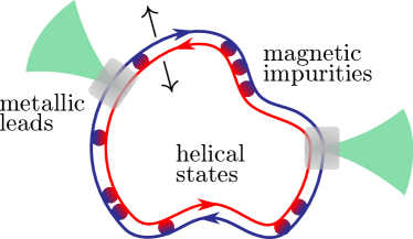
Figure 1: (Color online) Helical edges states tunnel-coupled to the metallic point contacts. The magnetic impurities are marked by dots.

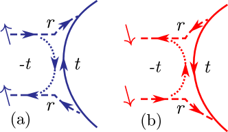
Figure 2: (Color online) Non-magnetic point contact between the helical ring and the spinful wire. Different spin projections (shown by blue and red color) do not mix at the contact and correspond to electrons propagating along the helical edge in the opposite directions. The spin-independent amplitudes $t$ and $r$ obey $t^{2}+r^{2}=1$.

We will study both classical and quantum contributions to the spin polarization. The quantum contribution is sensitive to magnetic field due to the AB effect. Hence our setup represents an example of AB interferometer built on HES. The form and shape of the AB oscillations strongly depend on the relation between temperature $T$ and level spacing $\Delta=2\pi v_{F}/L,$ which is controlled by total interferometer circumference $L$ and the Fermi velocity $v_{F}.$ Let us do some estimates. For $L=10~{}\mu$m and $v_{F}=10^{7}$ cm/s, we get $\Delta\approx 3$ K. As seen from this estimate, the case

$$T\gg\Delta$$ (5)

is much more interesting for possible applications. We will focus on this case throughout the article. There is also upper limitation for temperature. For good quantization, $T$ should be much smaller than the bulk gap of the topological insulator: $T\ll\Delta_{\rm b}$. For the first time quantum spin Hall effect was observed in structures based on HgTe/CdTe Konig et al. (2007) and InAs/GaSb Knez et al. (2011), which had a rather narrow bulk gap, less than 100 K. Substantially large values were observed recently in WTe${}_{2},$ where gap of the order of 500 K was observed Wu et al. (2018), and in bismuthene grown on a SiC (0001) substrate, where a bulk gap of about 0.8 eV was demonstrated Reis et al. (2017); Li et al. (2018) (see also recent discussion in Ref. Stühler et al. (2020)). Thus, recent experimental studies unambiguously indicate the possibility of transport through HES at room temperature, when the condition $\Delta_{\rm b}\gg T\gg\Delta$, needed for applicability of our theory, can be easily satisfied. Importantly, this condition ensures the universality of spin and charge transport (see discussion in Ref. Niyazov et al. (2018)), which do not depend on details of the systems, in particular, on the device geometry.

II.3 Tunneling conductance

Recently, we discussed dependence of the tunneling conductance $G$ of such a setup on the external magnetic flux $\Phi$ piercing the area encompassed by edge states Niyazov et al. (2018). For consistency, we briefly summarize main results of Ref. Niyazov et al. (2018) here. We have demonstrated the existence of interference-induced effects, which are robust to the temperature, i.e. survive under the condition Eq. (5), and can therefore be obtained for relaxed experimental conditions (for discussion of this regime in conventional interferometers see Refs. Jagla and Balseiro (1993); Dmitriev et al. (2010); Shmakov et al. (2013); Dmitriev et al. (2015, 2017)). Specifically, we have found that $G$ is structureless in ballistic case but shows periodic dependence on dimensionless flux $\phi=\Phi/\Phi_{0}$ (here, $\Phi_{0}=hc/e$ is the flux quantum), with the period $1/2,$ in the presence of a single magnetic impurity in one of the interferometer’s shoulders. Such a weak impurity can be taken into account perturbatively provided that $\theta\ll\rm{max}(\lambda,1).$ The resulting analytical expression for the transmission coefficient reads Niyazov et al. (2018)

$$\mathcal{T}=\tanh\lambda-\frac{{\tilde{\theta}}^{2}}{2}\tanh^{2}\lambda$$ (6)

where ${\tilde{\theta}}^{2}={\theta}^{2}(1+\mathcal{C}|_{\theta=0})$ and

$${\cal C}=\frac{t^{4}e^{4i\pi\phi}}{1-t^{4}\cos^{2}\theta e^{4i\pi\phi}}+\frac{t^{4}e^{-4i\pi\phi}}{1-t^{4}\cos^{2}\theta e^{-4i\pi\phi}},$$ (7)

represents “ballistic Cooperon” Niyazov et al. (2018) which is the interference contribution of the processes in which the electron wave splits at the impurity into two parts passing the setup in the opposite directions and returning to impurity after a number of revolutions with equal winding numbers (see Fig. 6 of Ref. Niyazov et al. (2018)). The factor

$$\frac{{\tilde{\theta}}^{2}}{{\theta}^{2}}=1+{\cal C}|_{\theta=0}=\frac{\sinh(4\lambda)}{\cosh(4\lambda)-\cos(4\pi\phi)},$$ (8)

describes coherent enhancement of backscattering probability caused by multiple returns to the impurity. This enhancement has a purely quantum nature. The classical limit, when all interference processes are neglected, can be obtained by averaging $\mathcal{T}$ over flux. Having in mind that $\langle\mathcal{C}\rangle_{\phi}=0,$ we find that ”classical” conductance is given by Eq. (6) with the replacement ${\tilde{\theta}}^{2}\to\theta^{2}.$ Hence, in the perturbative regime, $\mathcal{T}$ obeys $1/2-$flux periodicity $\mathcal{T}(\phi+1/2)=\mathcal{T}(\phi)$ and shows sharp identical antiresonances at integer and half-integer values of $\phi$ in the limit of weak tunneling coupling, $\lambda\ll 1.$ In the latter limit, the non-perturbative effects lead to appearance of the additional contribution $2\theta^{2}.$ in the denominator of Eq. (8) Niyazov et al. (2018). Physically, this corresponds to the broadening of the antiresonances because of multiple coherent scattering events.

II.4 Spin polarization

Next, we discuss the spin polarization of outgoing electrons. We will limit ourselves with discussion of non-interacting electrons focusing on high temperature case. For discussion of spin polarization in the low temperatures case see Refs. Chu et al. (2009); Masuda and Kuramoto (2012); Dutta et al. (2016); Björnson and Black-Schaffer (2018); Zhou et al. (2019), while interaction-induced Ronetti et al. (2016) and quantum pumping generated Ronetti et al. (2017) spin currents were considered for Fabry-Pérot geometry at $\phi=0.$ We will demonstrate that the finite polarization appears even in the fully classical regime and therefore robust to dephasing. There also exists quantum contribution to polarization which survives at relatively large temperature and is tunable by magnetic flux piercing the interferometer. Specifically, we will demonstrate that similar to tunneling conductance the quantum contribution to the polarization shows sharp identical resonances as a function of magnetic flux with maxima (in the absolute value) at integer and half-integer values of the flux.

In order to illustrate our approach, we consider a single impurity placed in the upper shoulder of the interferometer and discuss a simple limiting case: $\lambda=\infty,~{}\theta=\pi/2$ (strong impurity, open interferometer). In this case, $t=0$ and $r=1,$ so that electrons with spin up (down) can go only through upper (lower) shoulder of interferometer (see Fig. 2). On the other hand probability of backscattering by the impurity is given by $\sin^{2}\theta=1,$ so that impurity fully blocks transmission through the upper shoulder (see Fig. 3). Hence, such a setup serves as ideal spin filter: the transmission of electrons with spin up is blocked while spin-down electrons can freely pass through the interferometer. Consequently, the outgoing polarization reaches 100%. Evidently, this is a classical result which is not sensitive to dephasing. At the same time, fully polarized electron beam corresponds to a pure quantum spin state. In other words, even in the classical regime, the interferometer can create pure quantum states within the discussed limiting case. Below, we present detailed calculations of the spin polarization for a number of other cases.

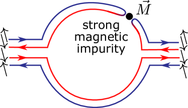
Figure 3: (Color online) Strong magnetic impurity blocks transmission of one component of the electron spin. For open setup, $\lambda=\infty,$ this leads to 100% polarization. Polarization reverses sign, when strong impurity is moved from upper to lower shoulder.

Results of Ref. Niyazov et al. (2018) can be easily generalized for calculation of spin polarization. For a weak impurity placed in the upper shoulder of interferometer, direct summation of amplitudes in a full analogy with Ref. Niyazov et al. (2018) yields in the lowest order in $\theta^{2}$:

$$T_{\alpha\beta}=\delta_{\alpha\beta}\tanh\lambda-\frac{\alpha\beta\exp[\lambda(\alpha+\beta)]}{4\cosh^{2}\lambda}~{}{\tilde{\theta}}^{2}$$ (9)

where $\alpha,\beta=\pm 1,$ for spin up and down, respectively. Classical probabilities $\langle T_{\alpha\beta}\rangle_{\phi}$ are given by Eq. (9) with the replacement ${\tilde{\theta}}^{2}\to\theta^{2}.$

The perturbative in $\theta^{2}$ spin polarization can be found from Eqs. (4) and (9):

$$P_{z}=-\frac{{\tilde{\theta}}^{2}}{2}=-\frac{\theta^{2}}{2}\frac{\sinh(4\lambda)}{\cosh(4\lambda)-\cos(4\pi\phi)}.$$ (10)

As is seen from this equation, polarization shows sharp identical antiresonances at integer and half-integer values of flux for weak tunneling coupling, $\lambda\ll 1,$ and weak AB oscillations for almost open setup, $\lambda\gg 1.$ Analogous calculation for a single impurity with the same strength, $\theta,$ placed in the lower shoulder of the interferometer yields Eq. (LABEL:Pz1) with the opposite sign. In the classical regime, the polarization is simply given by $P_{z}=\pm\theta^{2}/2,$ with the sign determined by the position of impurity. One can follow the evolution of polarization from quantum to classical case by introducing a dephasing process with the rate $\Gamma_{\varphi}$ which suppresses “ballistic Cooperon”. Technically, this means replacement $\lambda\to\lambda+\lambda_{\varphi}$ in Eq. (LABEL:Pz1), where $\lambda_{\varphi}=\pi\Gamma_{\varphi}/2\Delta$ (see Ref. Niyazov et al. (2018)). For $\lambda_{\varphi}\to\infty$ we restore the classical result. Away from the resonant points [more precisely, for $\cos(4\pi\phi)<0$], dephasing leads to the increase of polarization because the interference for such values of $\phi$ is destructive.

Microscopical calculation of $\Gamma_{\varphi}$ in HES is a non-trivial question. In conventional systems, including infinite single-channel quantum wires, dominates dephasing caused by electron-electron scattering. In HES, such dephasing is suppressed for the same reason as ordinary impurity backscattering. Nonzero (very slow) dephasing due to electron-electron interaction arises only when Rashba-type terms are present and slow energy dependence of these terms on energy is taken into account Schmidt et al. (2012); Kainaris et al. (2014). Additional suppression of the interaction-induced dephasing is expected due to finite geometry of the setup similar to the case of conventional single-channel interferometers Dmitriev et al. (2010). A very slow dephasing occurs due to the dynamics of the magnetic impurity. Such dynamics can arise due to the interaction directly with the conduction electrons Kurilovich et al. (2017) and due to the presence of a magnetic bath Niyazov et al. (2018). In the latter case, assuming that the averaged magnetic moment of impurity relaxes as $\langle\mathbf{M}(0)\mathbf{M}(t)\rangle=M^{2}\exp(-\Gamma_{0}t)$ one gets $\Gamma_{\varphi}=\Gamma_{0}$ Niyazov et al. (2018). Importantly, all proposed mechanisms lead to dephasing rate significantly slower (at least in the framework of theoretical models) than in conventional systems.

Let us now consider a setup with a number of randomly distributed impurities. We start our discussion with the classical regime ($\lambda_{\varphi}\to\infty$). One finds then $T_{\alpha\beta}$ as the sum over contributions from classical trajectories propagating clockwise and counterclockwise and experiencing collisions by magnetic impurities with forward probability $\cos^{2}\theta$ and backward probability $\sin^{2}\theta.$ Relations between classical currents flowing from different sides of the impurity read: $J_{n+1}^{\uparrow}=\cos^{2}\theta J_{n}^{\uparrow}+\sin^{2}\theta J_{n+1}^{\downarrow},$  $J_{n}^{\downarrow}=\sin^{2}\theta J_{n}^{\uparrow}+\cos^{2}\theta J_{n+1}^{\downarrow}.$ The vectors $\mathbf{J}_{n}=(J_{n}^{\uparrow},J_{n}^{\downarrow})$ and $\mathbf{J}_{n+1}=(J_{n+1}^{\uparrow},J_{n+1}^{\downarrow})$ are thus connected by the classical transfer matrix

$$\hat{W}_{cl}(\theta)=1+\tan^{2}\theta\hat{P},\quad\hat{P}=\left(\begin{array}[]{cc}-1&1\\ -1&1\\ \end{array}\right).$$ (11)

It obeys simple multiplication rule, $\hat{W}_{cl}(\theta_{1})\hat{W}_{cl}(\theta_{2})=\hat{W}_{cl}(\theta),$$\quad\tan^{2}(\theta)=\tan^{2}(\theta_{1})+\tan^{2}(\theta_{2}).$ Let us consider setup containing $N_{u}$ impurities in the upper shoulder, characterized by $\theta_{1},\ldots,\theta_{N_{u}}$ and $N_{l}$ in the lower one characterized by $\theta_{1}^{\prime},\ldots,\theta_{N_{u}}^{\prime}$. Due to multiplicativity property one can equivalently consider setup with two impurities having effective strengths $g_{u}=\sum^{N_{u}}_{n=1}\tan^{2}(\theta_{n})$, and $g_{l}=\sum^{N_{l}}_{n=1}\tan^{2}(\theta^{\prime}_{n}),$ placed respectively in the upper and lower shoulder of the interferometer. Next, we assume that current entering interferometer from the left contact is unpolarized, and use the scattering probabilities $r^{2}$ and $t^{2}$ to write balance equations for currents at the left and right contacts. We find

$$P_{z}=\frac{g_{l}-g_{u}}{2+(g_{u}+g_{l})\coth\lambda}.$$ (12)

Hence, the finite polarization exists even in the classical regime and is therefore robust to dephasing con .

Figure 4: (Color online) Broadening of resonances in polarization with increasing strength of magnetic disorder, $\rho^{2}=(N_{u}+N_{l})\rho_{0}^{2}/3$, and $\lambda=0.03$.

The above perturbative analysis of a single impurity case shows that all quantum effects are encoded in the renormalization of backscattering probability: $\theta^{2}\to{\tilde{\theta}}^{2}.$ Physically, it happens because such effects arise due to the interference of multiple returns to magnetic impurity along the ballistic trajectories propagating in opposite directions and having the same winding numbers. Therefore, generalization for the case of many impurities is trivial: one should expand Eq. (LABEL:Pcl) over impurities backscattering probabilities in lowest order and take into account the renormalization, Eq. (8). For the case of weak impurities of equal strength, we find that $\mathcal{T}$ is given by Eq. (6) with the replacement ${\tilde{\theta}}^{2}\to{\tilde{\theta}}^{2}(N_{u}+N_{l}),$ and the polarization reads

$$P_{z}=\frac{{\tilde{\theta}}^{2}(N_{l}-N_{u})}{2}~{}\underset{\lambda\ll 1}{\longrightarrow}~{}\frac{2\lambda\theta^{2}(N_{l}-N_{u})}{1-\cos(4\pi\phi)+8\lambda^{2}}.$$ (13)

One can generalize this formula in order to take into account non-perturbative effects with respect to impurity strength (still assuming $\theta<1$). Corresponding calculations are presented in the Suppl. Material. The result is shown in Fig. 4. As seen, non-perturbative effects lead to broadening of the resonances.

One of the most important conclusions of this section is universality of obtained results which was discussed previously in context of conductance calculation Niyazov et al. (2018). The final equation for polarization is not sensitive to geometry of device and details of the structure. Also, the Berry phase drops out from the final result. Physically, this happens due to our assumption $T\gg\Delta.$ In this case, quantum contribution to the conductance depends on quantum return probability (ballistic Cooperon) which is the universal quantity.

II.5 Ensemble of qubits

The transport through a HES-based interferometer was examined above (and earlier in Niyazov et al. (2018)) by a direct summation of the amplitudes of quantum transitions. Equivalently, the charge transfer through the interferometer can be viewed as a tunneling through an ensemble of equivalent qubits.

The latter approach is applicable for important case of either $\phi\ll 1$ or $\phi-1/2\ll 1$ and weak impurities. Although it does not allow one to describe transmission coefficient and polarization for $\phi\sim 1,$ it is more illustrative physically and much more suitable for the analysis of quantum computing in the system under discussion. Below, we discuss this approach for the case if the interferometer with a single magnetic impurity.

The key idea is that the tunneling amplitude through the interferometer can be presented as a sum of the transition amplitudes through intermediate states corresponding to quasistationary levels of an almost closed HES (similar approach for non-helical single-channel interferometer was discussed in Ref. Shmakov et al. (2013)). As a starting point, we consider an interferometer in the limit of an infinitely weak tunnel coupling, i.e. a system of two closed HES. In the absence of magnetic impurity, quantum levels are given by the following formula, $\epsilon^{\pm}_{n}(\phi)=\Delta(n\pm\phi),$ and for integer and half-integer values of the flux, the level system is degenerate: $\epsilon^{+}_{n}(0)=\epsilon^{-}_{n}(0),$ $\epsilon^{+}_{n}(1/2)=\epsilon^{-}_{n+1}(1/2).$ Magnetic impurities lift this degeneracy. In particular, for a single magnetic impurity described by Eq. (3), quantum levels are given by

$$\epsilon^{\pm}_{n}=\Delta(n\pm\phi_{0}),$$ (14)

where $\phi_{0}$ obeys

$$\cos(2\pi\phi_{0})=\cos\theta\cos(2\pi\phi),$$ (15)

hence, anticrossing at $\phi=0$ and $\phi=1/2.$ The energy levels are plotted in Figs. 5 (a,b). For weak impurity, splitting at anticrossing points, $(\epsilon^{+}-\epsilon^{-})|_{\phi=0}=2\Delta\theta,$ is small.

The form of wave functions, provided in Suppl. Material, shows that spinors corresponding to different $n$ have the same direction of local spins at the impurity position:

$$\mathbf{S}^{\alpha}(x_{0})=-\mathbf{S}^{-\alpha}(x_{0})=\frac{1}{2}\langle\psi_{n}^{\alpha}(x_{0})|\bm{\hat{\sigma}}|\psi_{n}^{\alpha}(x_{0})\rangle,\quad\alpha=\pm.$$

With increasing $x$ starting from $x=x_{0}+0,$ $z$-component of local spin does not change, $S_{z}^{\alpha}(x)=S_{z}^{\alpha}(x_{0}).$ By contrast, the perpendicular component of local spin rapidly rotates, rotating by angle $4\pi(n\pm\phi_{0})$ upon arrival to the point $x=x_{0}-0$ after passage of the ring.

Anticrossing at $\phi=0$ is illustrated in Fig. 5 (c) (picture at $\phi=1/2$ is fully analogous). For weak impurity, in vicinity of anticrossing point, we have

$$2\pi\phi_{0}\approx\sqrt{(2\pi\phi)^{2}+\theta^{2},}$$ (16)

and, consequently,

$$\delta\epsilon=\epsilon^{+}_{n}-\epsilon^{-}_{n}\approx 2\Delta\sqrt{\phi^{2}+(\theta/2\pi)^{2}},$$ (17)

for $\theta\ll 1,~{}\phi\ll 1.$ As seen, close to anticrossing points the distance between $(n,+)$ and $(n,-)$ is small, so levels are almost degenerate, and can be controlled either by perpendicular magnetic field, which effects both $\phi$ and $\theta,$ or by parallel field, which also rotates moment of the magnetic impurity thus changing $\theta.$ Close to points $\phi=0$ and $\phi=1/2$, $z-$component of spin changes very sharply (see Fig. 6)

$$S_{z}^{\pm}\approx\mp\frac{\pi\phi}{\sqrt{(2\pi\phi)^{2}+\theta^{2}}},\quad\text{for}~{}|\phi|\ll 1,~{}\theta\ll 1,$$ (18)

and similarly for $|\phi-1/2|\ll 1.$

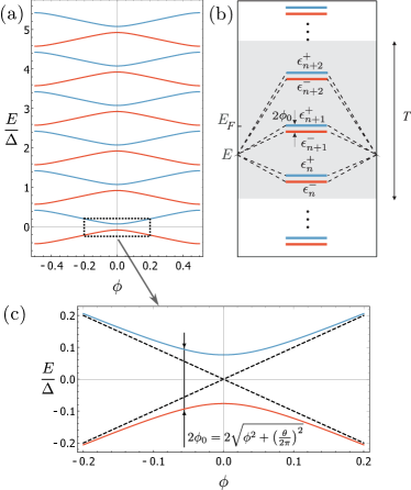
Figure 5: (Color online) (a) Energy levels of right- and left- moving electrons (red and blue curves, respectively) in the closed interferometer; (b) Transmission of the electrons through ensemble of $T/\Delta$ active qubits; (c) Anticrossing at $\phi=0.$

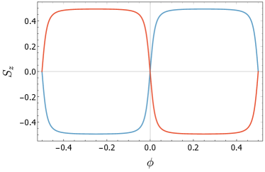
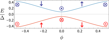
Figure 6: (Color online) Variation of qubit states with the magnetic flux. For $\phi=0$ both right- and left-moving electrons (red and blue curves, respectively) have spins perpendicular to the $z-$axis. Electron spin switches between $S_{z}=1$ to $S_{z}=-1$ within narrow interval of $\phi.$

For week tunneling coupling ($\lambda\ll 1$), the tunneling transport of the electrons through interferometer can be described in terms of transmission amplitudes (see Shmakov et al. (2013) and Suppl. Material)

$$A_{n}^{\alpha}(\epsilon)\propto\frac{1}{\epsilon-\epsilon_{n}^{\alpha}-i\Gamma/2}+\dots,$$ (19)

where $\Gamma\approx 2\Delta\lambda/\pi$ is the tunneling rate, and $+\dots$ stands for non-singular contribution. Both $\cal T$ and $P$ can be expressed in terms of energy-averaged bilinear combinations of these amplitudes. There are “classical” terms, $\propto\langle|A_{n}^{\alpha}(\epsilon)|^{2}\rangle_{\epsilon},$ and interference terms, $\propto\langle A_{n}^{\alpha}(\epsilon)A_{m}^{\beta*}(\epsilon)\rangle_{\epsilon}$ with $(n,\alpha)\neq(m,\beta),$ corresponding to transitions through different quantum levels (see Fig. 5b). For the case under discussion, $\lambda\ll 1,~{}T\gg\Delta,$ the interference contribution is dominated by terms with $n=m$ and $\beta=-\alpha,$

$$\left\langle A_{n}^{\alpha}(\epsilon)A_{n}^{-\alpha*}(\epsilon)\right\rangle_{\epsilon}\approx\frac{2\pi i}{\alpha\delta\epsilon+i\Gamma}\left(-\frac{\partial f_{F}}{\partial\epsilon}\right)_{\epsilon=n\Delta},$$ (20)

while interference processes with $n\neq m$ are described by similar equation which contain term $(n-m)\Delta\gg\delta\epsilon$ in the denominator and therefore is small.

II.6 Quantum computing by qubit ensemble

It is known that conventional interferometers with spin-orbit (SO) interaction (or an array of such interferometers) can be used as one-qubit quantum gates of various types (X-gate, Z-gate, phase gate, and Hadamard gate) Földi et al. (2005), which manipulate spin states of the electrons with given energy—the so-called flying qubits. The flying qubits can be used for quantum calculations at very low temperatures $<100$ mK Bäuerle et al. (2018). Analyzing analytical expression for energy- and spin-dependent transmission amplitudes $t_{\alpha\beta}(\epsilon)$ [see Eq. (31) of the Suppl. Material] one can—in a full analogy with Ref. Földi et al. (2005)—introduce quantum gates of different types. However, here we would like to focus on a different issue, namely, possibility of high-temperature qubit manipulation. Since, we consider almost closed tunneling interferometer, we will use language of the quantum levels introduced in the previous section.

The almost degenerate pairs of levels represent an ensemble of qubits with equal interlevel distance. The number of active qubits, which are able to participate in the spin and charge transport is given by

$${\cal N}_{\rm active}\simeq\frac{T}{\Delta}.$$ (21)

Transmission of charge and spin through the interferometer can be considered in terms of coherent hopping through these qubits (analogously to the case of conventional interferometer Shmakov et al. (2013)) as illustrated in Fig. 5b.

Technically, in order to describe transition though qubit levels one should introduce projection operators $\hat{P}_{1}$ and $\hat{P}_{2}$ (see Suppl. Material), which can be presented as

$$P_{1,2}=\frac{1}{2}(1\pm\hat{H})\,.$$

Here we introduced Hadamard operator

$$\hat{H}=\begin{pmatrix}a&be^{-i\xi}\\ be^{i\xi}&-a\end{pmatrix},$$ (22)

where coefficients $b={e^{-2\pi i\phi}\tan\theta}/{\sin(2\pi\phi_{0})}$ and $a=i\left[e^{-2\pi i\phi}/\cos\theta-\cos(2\pi\phi_{0})\right]/\sin(2\pi\phi_{0})$, obey $a^{2}+b^{2}=1$ and depend on the strength of the impurity and the magnetic flux only, while the dependence on the energy is encoded in the exponents $e^{\pm i\xi}$ entering off-diagonal terms of $\hat{H}.$ The operator $\hat{H}$ has standard properties

$$\hat{H}^{2}=1,\quad{\rm Tr}~{}\hat{H}=0,\quad{\rm det}~{}\hat{H}=-1.$$ (23)

Importantly, $\hat{H}$ can be tuned by the external magnetic field.

Off-diagonal elements of $\hat{H}$ rapidly oscillate with energy and, strictly speaking, one could introduce a set of Hadamard operators corresponding to different quantum levels in the interferometer: $\hat{H}_{n\alpha}=\hat{H}_{\epsilon=\epsilon_{n\alpha}}.$ However, the results of direct calculations for conductance and spin polarization show that the dependence on $n$ drops out. Hence, we have an ensemble of qubits, which give coherent contributions to the charge and spin transport.

For $\theta\ll 1,\lambda\ll 1,$ and $\phi\ll 1,$ the transmission coefficient and polarization are expressed in terms of $\hat{H}$ as follows (see Suppl. Material)

$$\mathcal{T}\approx\frac{\pi\Gamma}{8\Delta}{\rm Tr}(\hat{A}),\qquad{P}_{z}\approx\frac{\pi\Gamma}{8\Delta\mathcal{T}}{\rm Tr}(\hat{\sigma}_{z}\hat{A}),$$ (24)

where $\Gamma=4\lambda v_{F}/L=2\lambda\Delta/\pi$ is the tunneling rate and

$$\hat{A}=\frac{\hat{S}(\Gamma+i\delta\epsilon\,\hat{H})^{\dagger}\hat{S}(\Gamma+i\delta\epsilon\,\hat{H})}{\Gamma^{2}+\delta\epsilon^{2}}+\frac{2\pi\Gamma}{\Delta}\hat{\sigma}_{z},$$ (25)

where information about tunneling coupling is encoded in $\Gamma$ and in the matrix

$$\hat{S}=\begin{pmatrix}e^{-\lambda}&0\\ 0&e^{\lambda}\end{pmatrix}.$$ (26)

Hence, measurement of $\mathcal{T}$ and $P_{z}$ allows one to read out information about ensemble of qubits. Importantly, the results of calculation do not depend on energy (entering through factor $\xi$). In other words, all qubits give equal contributions to conductance and polarization.

Using Eq. (22), for small $\theta,\lambda,$ and $\phi,$ we get

$$\mathcal{T}\!\approx\!\lambda\!-\!\frac{\lambda^{3}\theta^{2}}{4\lambda^{2}\!+\!\theta^{2}\!+\!4\pi^{2}\phi^{2}},~{}P_{z}\!\approx\!-\frac{\lambda\theta^{2}}{4\lambda^{2}\!+\!\theta^{2}\!+\!4\pi^{2}\phi^{2}}$$ (27)

The same equations are valid for $\phi$ close to $1/2$ with the replacement $\phi\to\phi-1/2.$ One can check by direct calculation that dependence on $\xi,$ and, consequently, on energy drops out after taking trace in Eqs. (24). We see that the approach based on qubit representation not only reproduces results obtained by direct summation of the amplitudes within $\theta^{2}$ precision but also allows one to perform non-perturbative summation over relevant scattering processes and to get $\theta^{2}$ in the denominator of Eqs. (27). Sharp dependence of $\mathcal{T}$ and $P_{z}$ on $\phi$ reflects tunability of the ensemble of qubits by external magnetic field.

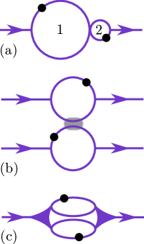
Figure 7: (Color online) Several setups containing two AB interferometrs: (a) Setup for one-qubit operations based on interferometers of different sizes connected in series. Interferometer of larger size is more sensitive to magnetic field and is used to manipulate the qubit spin state in the interferometer of smaller size (see also Fig. 8); (b) Setup for two-qubit operation based on interferometers connected in parallel and coupled by electron-electron interaction (the interaction region is marked by grey color); (c) Setup for creation of pure state of arbitrary polarization with two interferometers containing strong impurities that block transmission through corresponding shoulders of each interferometer and with joint contacts to metallic leads allowing for coherent tunneling to both interferometers.

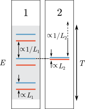
Figure 8: (Color online) Energy levels in setup with two interferometers of different sizes connected in series (see Fig. 7a). Energy levels in the interferometer of larger size are much more sensitive to magnetic field and can be tuned to manipulate a polarization of a single active qubit in the interferometer of smaller size.

It is interesting to discuss possible generalizations of the high-temperature computing schemes to more complex systems involving several interferometers based on HES or HES arrays. (Experimental study of HES arrays has recently begun Maier et al. (2017).) The simplest examples of setups with two interferometers are shown in Fig. 7. Figure  7a schematically depicts two interferometers tunnel-connected in series to leads and to each other, with different edge lengths $L_{1}$ and $L_{2}$ ($L_{1}\gg L_{2}$). In the absence of magnetic field, level spacings in these interferometers are very different: $\Delta_{1}\propto 1/L_{1}\ll\Delta_{2}\propto 1/L_{2}.$ Then, for $\Delta_{1}\ll T\ll\Delta_{2},$ there are $T/\Delta_{1}$ active qubits in the first interferometer and single active qubit in the second one (see Fig. 8). On the other hand, for weak impurities, spacing between qubit’s levels is much larger in the first interferometer, $2\Delta_{1}\phi_{1}\propto L_{1}\gg 2\Delta_{2}\phi_{2}\propto L_{2}$ (here, we assume that homogeneous magnetic field is applied to both systems, so $\phi_{1,2}\propto L_{1,2}^{2}$). Hence, the first interferometer is much more sensitive to magnetic field. In particular, one can tune an energy level in the system 1 to be in the resonance with the levels of active qubit in the system 2. Then, one can change the pure quantum state of the qubit 2 by very small variation of the external field.

Similar to the low-temperature case Bautze et al. (2014); Bäuerle et al. (2018); Bordone et al. (2019); Bellentani et al. (2020); Chen et al. (2014) one can suggest two qubit manipulation schemes taking into account the electron-electron interaction. To this end, one can use interferometers connected in parallel and coupled by interaction (see Fig.  7b). The most essential feature of the high-temperature case distinguishing it from the low-temperature one is that now effective manipulation is possible for the whole ensemble of qubits. In particular, simplest capacitive interaction between two interferometers would lead to the respective interaction-induced phase shift between states in the upper and down systems.

Finally, one can construct a setup for creation of outgoing polarized state with arbitrary polarization direction by using two interferometers containing strong impurities that block transmission through corresponding shoulders of each interferometer and with joint contacts to metallic leads allowing for coherent tunneling to both interferometers (see Fig.  7c). Assuming that unpolarized electrons enter the system from the left contact, we find that at the right contact there is interference of two pure coherent states with various (in general, arbitrary) polarizations. As a result, outgoing electrons will be polarized with the direction different from outgoing polarization of each interferometer.

III Conclusions

We have studied coherent spin transport through HES of 2D topological insulators. We have shown that unpolarized incoming electron beam entering the HES through one of the metallic leads acquires a finite polarization after transmission through the setup containing magnetic impurities. The finite polarization appears even in the fully classical regime and is therefore robust to dephasing. There also exists quantum contribution which survives at relatively high temperature and is tunable by magnetic flux piercing the area encompassed by HES. Specifically, the quantum contribution shows sharp identical AB resonances as a function of magnetic flux with maxima (in the absolute value) at integer and half-integer values of the flux. For the setup with a single strong magnetic impurity blocking the transmission in one shoulder of AB interferometer, and for large tunneling coupling, the spin polarization of transmitted electrons can achieve 100%, which implies that outgoing electrons are in the pure quantum spin state. Also this means that polarization can be transferred over distances on the order of the system size. The polarization reverses sign when impurity is moved from one shoulder of interferometer to another.

We discuss possible application of obtained results for quantum computing. We demonstrate that tunneling interferometer based on HES can be described in terms of ensemble of flux-tunable qubits giving equal contributions to conductance and spin polarization. Specifically, in presence of magnetic impurities and magnetic field the initially doubly degenerate HES spectrum is split so that the appearing pairs of quantum states act as qubits with the spin orientation easily tuned by magnetic flux. The number of active qubits participating in the charge and spin transport is given by the ratio of the temperature and the level spacing. The interferometer can effectively operate at high temperature and can be used for quantum calculations. In particular, the ensemble of qubits can be described by a single flux-tunable Hadamard operator. These findings are not sensitive to details of the system such as geometry of the HES and allows one to speak about single-qubit operations such as X or Z gate. Since we also predict the polarized state after passing the AB interferometer by the unpolarized beam, we can prepare the qubits in the desired states.

If one uses the outgoing polarized state as the input for the next AB interferometer, then one can further manipulate the states of the qubits. Arranging the setups involving several interferometers of certain geometries we can produce non-trivial two-qubit operations needed for quantum computations. The obtained results open wide avenue for applications in the area of quantum computing.

IV Acknowledgements

The work was supported by the Russian Science Foundation (Grant No. 20-12-00147) and by Foundation for the Advancement of Theoretical Physics and Mathematics “BASIS”. Work in Poland was supported by the Foundation for Polish Science through the grant MAB/2018/9 for CENTERA.

Supplemental material

In this Supplemental Material, we provide a short discussion of the Rashba coupling effects, derive an analytical expression for the transfer matrix of the interferometer, and analyze the spin polarization for the case of a large number of weak, randomly distributed magnetic impurities.

I Rashba coupling

The Rashba coupling is described by the following term in the Hamiltonian

$${\cal H}_{\rm Rashba}=\sum\limits_{\alpha,\beta=\uparrow,\downarrow}\psi_{\alpha}^{\dagger}{\sigma}_{\alpha\beta}^{y}\{a(x),i\partial_{x}\}\psi_{\beta},$$ (28)

where $a(x)\,\mathbf{n}$ is the local Rashba field, $\mathbf{n}$ is the unit vector perpendicular to the plane of the topological insulator, and $\{\cdots\}$ stands for anticommutator Kimme et al. (2016). Assuming that the edge is smooth at the scale $p_{F}$ and $a(x)\ll v_{F}$, we can use the semiclassical arguments and integrate Schrödinger equation, corresponding to the Hamiltonian of HES, exactly. Such analysis was performed in Ref. Shmakov et al. (2012) for conventional (non-helical) materials and showed the appearance of Berry phase upon the whole revolution around the edge. It was shown however in Ref. Niyazov et al. (2018) that for our purposes and thanks to nature of helical edge states, the Berry phase is irrelevant.

Figure 9: Helical edge states without (a) and with (b) Rashba coupling. (Color online)

Let us calculate the phase acquired by the electron wave after a full revolution around the setup shown in Fig. 1. In order to make the physical picture more transparent, we consider first a general case with two chiralities (direction of propagation) and two spins not necessarily aligned with momentum (this case corresponds to a conventional single-channel spinful wire). The acquired phase includes three terms: a dynamical contribution $kL$ (here $k$ is the electron wave vector), magnetic phase $\pm 2\pi\phi$ and the Berry’s phase $\pm\delta$ Berry (1984), given by one half of the solid angle, subtended by spin direction during circumference of the interferometer. The dynamical contribution depends on $L$ only and does not change its sign when changing the chirality and spin projection. By contrast, the sign of magnetic phase is insensitive to spin but changes sign with changing the chirality. The Berry’s phase changes sign both with changing the chirality and with changing the spin (see Tab. 1). For helical edge only two out of four electron states are present, which are marked by boldface in the Table 1.

		chirality
		+	–
spin	$\uparrow$	$kL+\phi+\delta$	$kL-\phi-\delta$
	$\downarrow$	$kL+\phi-\delta$	$kL-\phi+\delta$

Table 1: Phases of electron wave function after a full revolution in the arbitrary setup shown in Fig.  1.

Analyzing the corresponding phases we arrive at a conclusion, which is of key importance for our analysis. Information about the geometrical structure of the edge states, in particular, about curvature of the edge and/or non-planar geometry, is encoded in the Berry’s phase, but as we see, it is simply added to the dynamical phase, which implies that amplitude of any process depends on $kL+\delta.$ This, in turn, means that tunneling conductance for a given energy (i.e. before thermal averaging) depends on the Berry’s phase and is, therefore, sensitive to geometry of the setup. However, for $T\gg\Delta,$ the thermal averaging implies integration over $k$ within a wide interval, $\delta k\sim T/\hbar v_{F}\gg 1/L,$ around the Fermi wave vector $k_{F}.$ After changing integration variable, $k+\delta/L\to k^{\prime}$, the Berry’s phase drops out with the exponential precision. This should be contrasted to the case of conventional interferometers with weak SO coupling, where the Berry’s phase contributes to the Aharonov-Casher phase and strongly effects both $\mathcal{T}(\epsilon)$ and energy-averaged transmission coefficient, $\mathcal{T}$ Shmakov et al. (2012). Physically, this happens because for weak SO coupling, the electron wave with a given spin polarization can propagate both clockwise and counterclockwise and the phase shift between such waves with equal winding numbers, $n_{1}=n_{2}=n$, is given by $2(\phi+\delta)n$.

The conclusion formulated above requires a minor comment. As seen from the Fig. 9, spin rotates while an electron passes the interferometer. The parameter $\theta$ which determines the scattering strength depends on the direction of magnetic moment of the impurity with respect to the local spin quantization axis. The direction of outgoing polarization is also parallel to the local quantization axis at the position of outgoing contact.

II Transitions through energy levels of closed ring

Here we derive analytical expressions describing anticrossing of quantum levels of right- and left-moving electrons on the example of a single impurity placed in the upper shoulder. We consider interferometer with the lengths of the upper and lower shoulders given by $s$ and $L-s,$ respectively. The magnetic impurity is placed at position $x_{0}$ such that $0<x_{0}<s.$ Using expression for scattering matrix (3), one can easily find transfer matrix of impurity

$$\hat{W}=\frac{e^{-i\alpha}}{\cos\theta}\left(\begin{array}[]{cc}1&i\sin\theta e^{-i\xi}\\ -i\sin\theta e^{i\xi}&1\end{array}\right),$$ (29)

where $\xi=\varphi+2kx_{0}.$ In this supplementary we may add the constant value of forward scattering phase $\alpha$ to the flux $2\pi\phi$ and set $\alpha=0$ below. The solution of the scattering problem for the electron with momentum $k$ on the whole system yields

$$\begin{pmatrix}a^{\uparrow}\\ a^{\downarrow}\end{pmatrix}=\hat{t}\begin{pmatrix}b^{\uparrow}\\ b^{\downarrow}\end{pmatrix}$$ (30)

where $(b^{\uparrow},b^{\downarrow})$ and $(a^{\uparrow},a^{\downarrow})$ are the amplitudes of incoming (from the left contact) and outgoing (to the right contact) waves and

$$\hat{t}=(1-e^{-2\lambda})e^{2\pi i\phi s/L}\begin{pmatrix}e^{iks}&0\\ 0&e^{-iks}\end{pmatrix}\begin{pmatrix}1&0\\ 0&e^{\lambda}\end{pmatrix}\hat{g}\begin{pmatrix}1&0\\ 0&e^{\lambda}\end{pmatrix},$$ (31)

where

$$\hat{g}=\frac{1}{1-\hat{W}\hat{\Lambda}}\hat{W}\begin{pmatrix}1&0\\ 0&-1\end{pmatrix},$$ (32)

$$\hat{\Lambda}=\begin{pmatrix}e^{i(QL+2\pi\phi)}&0\\ 0&e^{i(-QL+2\pi\phi)}\end{pmatrix},$$ (33)

and $Q$ is found from the condition $t^{2}e^{ikL}=e^{iQL},$ yielding

$$Q=k+i\frac{2\lambda}{L}.$$ (34)

The transmission coefficient and the spin polarization are expressed in terms of matrix $\hat{t}$ as follows

$$\mathcal{T}=\frac{1}{2}\left\langle{\rm Tr}\left(\hat{t}\hat{t}^{\dagger}\right)\right\rangle_{\epsilon},$$ (35)

$$\mathcal{P}=\frac{1}{2\mathcal{T}}\left\langle{\rm Tr}\left(\hat{t}\sigma_{z}\hat{t}^{\dagger}\right)\right\rangle_{\epsilon},$$ (36)

where $\langle\dots\rangle_{\epsilon}$ stands for thermal averaging. Here we neglect the Rashba coupling and assume that the incoming electrons are unpolarized. The matrix $\hat{g}$ can be presented as follows

$$\hat{g}=\cos\theta\left[\frac{\hat{P}_{1}}{1-e^{i(QL+2\pi\phi_{0})}}+\frac{\hat{P}_{2}}{1-e^{i(QL-2\pi\phi_{0})}}+\begin{pmatrix}0&0\\ 0&-1\end{pmatrix}\right],$$ (37)

where $\phi_{0}$ is found from

$$\cos(2\pi\phi_{0})=\cos\theta\cos(2\pi\phi)$$ (38)

and

$$\hat{P}_{1}=\frac{1}{2i\sin(2\pi\phi_{0})\cos\theta}\begin{pmatrix}-e^{-2i\pi\phi}+e^{2i\pi\phi_{0}}\cos\theta&ie^{-i(\xi+2\pi\phi)}\sin\theta\\ ie^{i(\xi-2\pi\phi)}\sin\theta&e^{-2i\pi\phi}-e^{-2i\pi\phi_{0}}\cos\theta\end{pmatrix},$$ (39)

$$\hat{P}_{2}=-\frac{1}{2i\sin(2\pi\phi_{0})\cos\theta}\begin{pmatrix}-e^{-2i\pi\phi}+e^{-2i\pi\phi_{0}}\cos\theta&ie^{-i(\xi+2\pi\phi)}\sin\theta\\ ie^{i(\xi-2\pi\phi)}\sin\theta&e^{-2i\pi\phi}-e^{2i\pi\phi_{0}}\cos\theta\end{pmatrix}.$$ (40)

These are projection operators obeying: $\hat{P}_{1}^{2}=\hat{P}_{1},~{}\hat{P}_{2}^{2}=\hat{P}_{2},~{}\hat{P}_{1}\hat{P}_{2}=0,~{}\hat{P}_{1}+\hat{P}_{2}=1.$ Due to these properties, we can introduce Hadamard operator

$$\hat{H}=\hat{P}_{1}-\hat{P}_{2},$$ (41)

which obeys the standard property $\hat{H}^{2}=1.$ However, in contrast to conventional case, we have $H\neq H^{\dagger}.$ We can now write

$$\hat{P}_{1}=\frac{1+\hat{H}}{2},\quad\hat{P}_{2}=\frac{1-\hat{H}}{2}.$$ (42)

Thus defined Hadamard operator describes the isolated system and does not contain any information about tunneling coupling. We use now the following identities valid for arbitrary complex number $z$ with $\mbox{Im\,}z>0$ and arbitrary $\chi\in[0,1)$:

$$\frac{e^{i\chi z}}{1-e^{iz}}=\left\{\begin{array}[]{c}i\sum\limits_{n=-\infty}^{\infty}\frac{e^{2\pi i\chi n}}{z-2\pi n},\quad\text{for}~{}0<\chi<1,\\ i\sum\limits_{n=-\infty}^{\infty}\frac{1}{z-2\pi n}+\frac{1}{2},\quad\text{for}~{}\chi=0\end{array}\right.$$ (43)

Using Eqs. (42) and (43), we get

$$\hat{g}=\frac{i\cos\theta}{2}\left[-i\hat{\sigma}_{z}+\frac{\Delta}{2\pi}\sum\limits_{n,\alpha}\frac{1+\alpha\hat{H}}{\epsilon-\epsilon_{n}^{\alpha}+i\gamma/2}\right],$$ (44)

with $\gamma=4\lambda v_{F}/L=2\lambda\Delta/\pi.$

For completeness, we provide here the explicit form of wave functions for the energy levels (14)

$$\psi_{n}^{\pm}(x)=\frac{1}{\sqrt{|A^{\pm}|^{2}+|B^{\pm}|^{2}}}\left[\!\begin{array}[]{c}e^{ik_{n}^{\pm}(x-x_{0})}A^{\pm}\\ e^{-ik_{n}^{\pm}(x-x_{0})}B^{\pm}\end{array}\!\right]$$ (47)

Here, $\pm$ labels energy levels [see Eq. (14)], $k_{n}^{\pm}=\epsilon^{\pm}_{n}/v_{F},$ $A^{\pm}=\sin\theta e^{-i(\varphi\pm 2\pi\phi_{0})},$ $B^{\pm}=\cos\theta\sin(2\pi\phi)\pm\sin(2\pi\phi_{0}),$ and $\varphi$ is the angle describing position of the magnetic moment of the impurity with a fixed projection on the local electron spin. Orthogonality condition reads

$$\int\limits_{0}^{L}dx\langle\psi_{n}^{\alpha}(x)|\psi_{m}^{\beta}(x)\rangle=\delta_{nm}\delta_{\alpha\beta},\quad\alpha,\beta=\pm$$

We emphasize that coefficients $A^{\pm}$ and $B^{\pm}$ that determines direction of local spin at $x=x_{0}$ do not depend on $n.$

III Averaging over positions of impurities

Next, we find non-perturbative expressions for spin polarization assuming that $\rho_{0}^{2}N_{u}\ll 1,~{}\rho_{0}^{2}N_{l}\ll 1.$ In this case, the mean free path is much larger than $L,$ so that the regime is ballistic and one can neglect localization effects. We consider shoulders of equal length and replace interaction with $N_{u}$ ($N_{l}$) impurities in the upper (lower) shoulder by transfer matrix $\hat{W}_{u}$ ($\hat{W}_{l}$) describing scattering on the shoulder as a whole. In the ballistic regime, parameters of this matrix read

$$\theta_{u}e^{i\varphi_{u}}=\rho_{0}\sum\limits_{n=1}^{N_{u}}\sin\eta_{n}e^{i\varphi_{n}-2ikx_{n}},\quad\alpha_{u}=\rho_{0}\sum\limits_{n=1}^{N_{u}}\cos\eta_{n}$$ (48)

(and $u\to l$ for lower shoulder). We average the final polarization over directions of vectors $\mathbf{M}_{n},$ which means averaging over $\varphi_{n}$ and $\eta_{n}.$ The parameters of transfer matrix depend on positions of impurities, $x_{n}$. These positions, however, can be incorporated into $\varphi_{n}$ and drop out after averaging.

Let us consider interferometer with two effective impurities in the upper and lower shoulder, characterized by transfer matrices $\hat{W}_{u}=\hat{W}_{u}(\theta_{u},\varphi_{u},\alpha_{u})$ and $\hat{W}_{l}=\hat{W}_{l}(\theta_{l},\varphi_{l},\alpha_{l}),$ respectively. Assuming that $\theta_{u,l}\ll 1$ and in the vicinity of the resonances, $\delta\phi=\phi-n\ll 1$ or $\delta\phi=\phi-(n+1/2)\ll 1$, we find the disorder-averaged spin polarization, $\overline{P_{z}}=\int P_{z}f_{u}f_{l}~{}du\,dl,$ where

$$P_{z}\!=\!\frac{\lambda(\theta_{l}^{2}-\theta_{u}^{2})}{4\lambda^{2}\!+\!{(2\pi\,\delta\phi\!+\!\alpha_{u}\!+\!\alpha_{l})^{2}\!}+|\theta_{u}e^{i\varphi_{u}}\!-\!\theta_{l}e^{i\varphi_{l}}|^{2}}\,.$$ (49)

and $f_{u}$, $f_{l}$ are distribution functions for parameters of matrices $\hat{W}_{u}$ and $\hat{W}_{l}$. We have, $f_{u}=f_{u}(\theta_{u},\varphi_{u},\alpha_{u})=\exp\left[-(\theta_{u}^{2}+\alpha_{u}^{2})/(2\rho_{u}^{2})\right]/(2\pi)^{3/2}\rho_{u}^{3},$ with $\rho_{u}^{2}={N_{u}\rho_{0}^{2}/3}$. The function $f_{u}$ does not depend on $\varphi_{u}$ and is normalized as $\int f_{u}du=1,$ where $du=\theta_{u}d\theta_{u}d\alpha_{u}d\varphi_{u}$. Expression for $f_{l}$ is obtained by replacement $u\to l$. [One can easily show that the same functions $f_{u,l}$ can be used for disorder averaging of classical formula, Eq.  (LABEL:Pcl).] In Fig. 4 we present the results of calculations for averaged polarization. We see that sharp resonances in polarization broaden with increasing the strength of magnetic disorder, $\rho^{2}=(N_{u}+N_{l})\rho_{0}^{2}/3$.

A single impurity with $S$ matrix, given by Eq. (3) of the main text, placed at position $x_{0}$ is described by the transfer matrix (29). Assuming the subsequent averaging over $\varphi$ we may conveniently redefine $\varphi=\varphi+\pi/2$. Having $N_{u}$ impurities at the upper shoulder, characterized by transfer matrices $\hat{W}_{1}$, …$\hat{W}_{N_{u}}$, we determine the transfer matrix of the whole upper shoulder as

$$\hat{W}_{u}=\hat{W}_{1}\hat{W}_{2}\ldots\hat{W}_{N_{u}},$$

and similarly for $\hat{W}_{l}$. In the weak impurity limit non-commutative property of $\hat{W}_{j}$ is relaxed and we obtain Eq. (48). We define 2$\times$2 matrices $\kappa=\mbox{diag}[e^{-\lambda/2},e^{\lambda/2}]$, $\Lambda_{1}=\mbox{diag}[e^{ikL/2+i\pi\phi},e^{-ikL/2+i\pi\phi}]$ and the matrix of transmission amplitudes

$$\hat{t}=2\sinh\lambda\;\Lambda_{1}\kappa\,\hat{W}_{u}\,\kappa\,(1-\kappa\,\Lambda_{1}^{2}\hat{W}_{l}\,\kappa^{2}\hat{W}_{u}\,\kappa)^{-1}\sigma_{3}\,.$$

The transmission coefficients are expressed via elements of $\hat{t}$ as follows: $T_{\alpha\beta}(\epsilon)=|t_{\alpha\beta}|^{2}$. Straightforward calculation leads then to Eq. (49).

Let us now calculate distribution functions for parameters of $\hat{W}_{u}$ and $\hat{W}_{l}.$ To this end, we enforce the conditions (48) above by writing

$$\int\frac{ds_{1}\,ds_{2}\,ds_{3}}{(2\pi)^{3}}e^{is_{1}(\theta_{u}\cos\varphi_{u}-\rho_{0}\sum\sin\eta_{n}\cos{(\varphi_{n}-2kLx_{n}}))}\times e^{is_{2}(\theta_{u}\sin\varphi_{u}-\rho_{0}\sum\sin\eta_{n}\sin{(\varphi_{n}-2kLx_{n}}))+is_{3}(\alpha_{u}-\rho_{0}\sum\cos\eta_{n})}.$$

Averaging over the orientation of impurities is given by $\prod_{n}{\sin\eta_{n}d\eta_{n}\,d\varphi_{n}}/{4\pi}$. Performing this integration and then integrating over $s_{1,2,3}$ in weak scatterers’ limit, we obtain the above formulas for $f_{u}$ and $f_{l}$. The average polarization is given by $\langle P_{z}\rangle=\int P_{z}f_{u}f_{l}~{}du\,dl$. We raise the denominator of $P_{z}$ to the exponent, $\lambda(\theta_{l}^{2}-\theta_{u}^{2})/(4\lambda^{2}\!+\ldots)=\lambda(\theta_{l}^{2}-\theta_{u}^{2})\int_{0}^{\infty}dz\,e^{-z(4\lambda^{2}\!+\ldots)}$ and perform integration over $du\,dl$. The remaining integration over $x=2z(\rho_{u}^{2}+\rho_{l}^{2})$ reads

$$\langle P_{z}\rangle=\lambda{\cal A}\int_{0}^{\infty}\tfrac{dx}{(1+x)^{5/2}}\exp\left[-\tfrac{2x}{\rho^{2}}\left(\lambda^{2}+\tfrac{\pi^{2}\delta\phi^{2}}{1+x}\right)\right]=\lambda{\cal A}\;F\left[{\pi\delta\phi}/\lambda,\rho/{2\lambda}\right]\,,$$

where

$$F\left[\Phi,z\right]=\tfrac{z^{2}}{2\Phi^{2}}\mbox{Re}\left[1-\sqrt{\tfrac{\pi}{2}}{e^{\frac{(1-i\Phi)^{2}}{2z^{2}}}\left(\tfrac{1}{z}-i\tfrac{z}{\Phi}\right)\mbox{erfc}\left[\tfrac{1-i\Phi}{\sqrt{2}z}\right]}\right]\,.$$ (50)

Here $\rho^{2}=\rho_{u}^{2}+\rho_{l}^{2}$ and asymmetry parameter ${\cal A}=(\rho_{u}^{2}-\rho_{l}^{2})/(\rho_{u}^{2}+\rho_{l}^{2})$. The compact form (50) was obtained by expanding general expressions at small $\lambda$, $\delta\phi$. Making substitution $\pi\,\delta\phi\to\frac{1}{2}\sin 2\pi\phi$ in (50), we restore the expected periodicity of $\langle P_{z}\rangle$. Thus obtained function is shown in Fig. 4 of the main text. It is a good approximation of $\langle P_{z}\rangle$ in the whole range of $\phi$.

References

- National Academies of Sciences et al. (2019) E. National Academies of Sciences, Medicine, E. Grumbling, and M. Horowitz, Quantum Computing: Progress and Prospects (The National Academies Press, Washington, DC, 2019).
- Zwanenburg et al. (2013) F. A. Zwanenburg, A. S. Dzurak, A. Morello, M. Y. Simmons, L. C. L. Hollenberg, G. Klimeck, S. Rogge, S. N. Coppersmith, and M. A. Eriksson, Rev. Mod. Phys. 85, 961 (2013).
- Wolf et al. (2001) S. A. Wolf, D. D. Awschalom, R. A. Buhrman, J. M. Daughton, S. Von Molnár, M. L. Roukes, A. Y. Chtchelkanova, and D. M. Treger, Science, Science 294, 1488 (2001).
- Žutić et al. (2004) I. Žutić, J. Fabian, and S. Das Sarma, Rev. Mod. Phys. 76, 323 (2004).
- Awschalom and Flatté (2007) D. D. Awschalom and M. E. Flatté, Nat. Phys. 3, 153 (2007).
- Datta and Das (1990) S. Datta and B. Das, Appl. Phys. Lett. 56, 665 (1990).
- Crooker et al. (2005) S. A. Crooker, M. Furis, X. Lou, C. Adelmann, D. L. Smith, C. J. Palmstrøm, and P. A. Crowell, Science 309, 2191 (2005).
- Appelbaum et al. (2007) I. Appelbaum, B. Huang, and D. J. Monsma, Nature 447, 295 (2007).
- Lou et al. (2007) X. Lou, C. Adelmann, S. A. Crooker, E. S. Garlid, J. Zhang, K. S. Reddy, S. D. Flexner, C. J. Palmstrøm, and P. A. Crowell, Nat. Phys. 3, 197 (2007).
- Koo et al. (2009) H. C. Koo, J. H. Kwon, J. Eom, J. Chang, S. H. Han, and M. Johnson, Science 325, 1515 (2009).
- Kum et al. (2012) H. Kum, J. Heo, S. Jahangir, A. Banerjee, W. Guo, and P. Bhattacharya, Appl. Phys. Lett. 100, 182407 (2012).
- Wunderlich et al. (2010) J. Wunderlich, B. G. Park, A. C. Irvine, L. P. Zârbo, E. Rozkotová, P. Nemec, V. Novák, J. Sinova, and T. Jungwirth, Science 330, 1801 (2010).
- Betthausen et al. (2012) C. Betthausen, T. Dollinger, H. Saarikoski, V. Kolkovsky, G. Karczewski, T. Wojtowicz, K. Richter, and D. Weiss, Science 337, 324 (2012).
- Schmidt et al. (2000) G. Schmidt, D. Ferrand, L. Molenkamp, A. Filip, and B. van Wees, Phys. Rev. B 62, R4790 (2000).
- An et al. (2012a) X.-T. An, Y.-Y. Zhang, J.-J. Liu, and S.-S. Li, New J. Phys. 14, 083039 (2012a).
- An et al. (2012b) X.-T. An, Y.-Y. Zhang, J.-J. Liu, and S.-S. Li, J. Phys. Condens. Matter 24, 505602 (2012b).
- Michetti and Recher (2011) P. Michetti and P. Recher, Phys. Rev. B 83, 125420 (2011), 1011.5166 .
- Battilomo et al. (2018) R. Battilomo, N. Scopigno, and C. Ortix, Phys. Rev. B 98, 075147 (2018).
- Zare (2019) M. Zare, J. Magn. Magn. Mater. 492, 165605 (2019), 1808.08379 .
- Wójcik et al. (2012) P. Wójcik, J. Adamowski, M. Wołoszyn, and B. J. Spisak, Phys. Rev. B 86, 165318 (2012).
- Slobodskyy et al. (2003) A. Slobodskyy, C. Gould, T. Slobodskyy, C. R. Becker, G. Schmidt, and L. W. Molenkamp, Phys. Rev. Lett. 90, 246601 (2003).
- Hauptmann et al. (2008) J. R. Hauptmann, J. Paaske, and P. E. Lindelof, Nat. Phys. 4, 373 (2008).
- Folk et al. (2003) J. A. Folk, R. H. Potok, C. H. Marcus, and V. Umansky, Science 299, 679 (2003).
- Wójcik et al. (2015) P. Wójcik, J. Adamowski, M. Wołoszyn, and B. J. Spisak, J. Appl. Phys. 118, 014302 (2015).
- Matityahu et al. (2017) S. Matityahu, A. Aharony, O. Entin-Wohlman, and C. A. Balseiro, Phys. Rev. B 95, 085411 (2017).
- Shmakov et al. (2012) P. M. Shmakov, A. P. Dmitriev, and V. Y. Kachorovskii, Phys. Rev. B 85, 75422 (2012).
- Tsai et al. (2013) W. F. Tsai, C. Y. Huang, T. R. Chang, H. Lin, H. T. Jeng, and A. Bansil, Nat. Commun. 4, 1500 (2013).
- Debray et al. (2009) P. Debray, S. M. Rahman, J. Wan, R. S. Newrock, M. Cahay, A. T. Ngo, S. E. Ulloa, S. T. Herbert, M. Muhammad, and M. Johnson, Nat. Nanotechnol. 4, 759 (2009).
- Das et al. (2012) P. P. Das, N. K. Bhandari, J. Wan, J. Charles, M. Cahay, K. B. Chetry, R. S. Newrock, and S. T. Herbert, Nanotechnology 23, 215201 (2012).
- Bhandari et al. (2013) N. Bhandari, M. Dutta, J. Charles, R. S. Newrock, M. Cahay, and S. T. Herbert, Adv. Nat. Sci.: Nanosci. Nanotechnol. 4, 013002 (2013).
- Kohda et al. (2012) M. Kohda, S. Nakamura, Y. Nishihara, K. Kobayashi, T. Ono, J. I. Ohe, Y. Tokura, T. Mineno, and J. Nitta, Nat. Commun. 3, 1082 (2012).
- Chuang et al. (2015) P. Chuang, S. C. Ho, L. W. Smith, F. Sfigakis, M. Pepper, C. H. Chen, J. C. Fan, J. P. Griffiths, I. Farrer, H. E. Beere, G. A. Jones, D. A. Ritchie, and T. M. Chen, Nat. Nanotechnol. 10, 35 (2015).
- Földi et al. (2005) P. Földi, B. Molnár, M. G. Benedict, and F. M. Peeters, Phys. Rev. B 71, 033309 (2005).
- Chen et al. (2014) W. Chen, Z.-Y. Xue, Z. Wang, R. Shen, and D. Y. Xing, Eur. Phys. J. B 87, 57 (2014).
- Bautze et al. (2014) T. Bautze, C. Süssmeier, S. Takada, C. Groth, T. Meunier, M. Yamamoto, S. Tarucha, X. Waintal, and C. Bäuerle, Phys. Rev. B 89, 125432 (2014).
- Bäuerle et al. (2018) C. Bäuerle, D. Christian Glattli, T. Meunier, F. Portier, P. Roche, P. Roulleau, S. Takada, and X. Waintal, Reports Prog. Phys. 81, 056503 (2018).
- Bordone et al. (2019) P. Bordone, L. Bellentani, and A. Bertoni, Semicond. Sci. Technol. 34, 103001 (2019).
- Bellentani et al. (2020) L. Bellentani, G. Forghieri, P. Bordone, and A. Bertoni, Phys. Rev. B 102, 035417 (2020), 2003.04050 .
- Stühler et al. (2020) R. Stühler, F. Reis, T. Müller, T. Helbig, T. Schwemmer, R. Thomale, J. Schäfer, and R. Claessen, Nat. Phys. 16, 47 (2020), 1901.06170 .
- Strunz et al. (2020) J. Strunz, J. Wiedenmann, C. Fleckenstein, L. Lunczer, W. Beugeling, V. L. Müller, P. Shekhar, N. T. Ziani, S. Shamim, J. Kleinlein, H. Buhmann, B. Trauzettel, and L. W. Molenkamp, Nat. Phys. 16, 83 (2020), 1905.08175 .
- com (a) See Ref. Dmitriev et al. (2010) for discussion of this problem in conventional interferometers.
- Kane and Mele (2005) C. L. Kane and E. J. Mele, Phys. Rev. Lett. 95, 226801 (2005).
- Bernevig et al. (2006) B. A. Bernevig, T. L. Hughes, and S. C. Zhang, Science 314, 1757 (2006).
- König et al. (2007) M. König, S. Wiedmann, C. Brüne, A. Roth, H. Buhmann, L. W. Molenkamp, X. L. Qi, and S. C. Zhang, Science 318, 766 (2007).
- Roth et al. (2009) A. Roth, C. Brüne, H. Buhmann, L. W. Molenkamp, J. Maciejko, X.-L. Qi, and S.-C. Zhang, Science 325, 294 (2009).
- Gusev et al. (2011) G. M. Gusev, Z. D. Kvon, O. A. Shegai, N. N. Mikhailov, S. A. Dvoretsky, and J. C. Portal, Phys. Rev. B 84, 121302 (2011).
- Brüne et al. (2012) C. Brüne, A. Roth, H. Buhmann, E. M. Hankiewicz, L. W. Molenkamp, J. Maciejko, X.-L. Qi, and S.-C. Zhang, Nat. Phys. 8, 485 (2012).
- Kononov et al. (2015) A. Kononov, S. V. Egorov, Z. D. Kvon, N. N. Mikhailov, S. A. Dvoretsky, and E. V. Deviatov, JETP Lett. 101, 814 (2015).
- Hasan and Kane (2010) M. Z. Hasan and C. L. Kane, Rev. Mod. Phys. 82, 3045 (2010).
- Qi and Zhang (2011) X.-L. Qi and S.-C. Zhang, Rev. Mod. Phys. 83, 1057 (2011).
- Kurilovich et al. (2017) P. D. Kurilovich, V. D. Kurilovich, I. S. Burmistrov, and M. Goldstein, JETP Lett. 106, 593 (2017).
- com (b) In Ref.Niyazov et al. (2018) we, for simplicity, considered the model of impurity with zero forward scattering phase, .
- com (c) Actually, is defined as and coincides with Eq. (4) in the case , see Eq. (9).
- com (d) Parameter is connected with tunneling transparency used in Niyazov et al. (2018) as follows: .
- Konig et al. (2007) M. Konig, S. Wiedmann, C. Brune, A. Roth, H. Buhmann, L. W. Molenkamp, X.-L. Qi, and S.-C. Zhang, Science (80-. ). 318, 766 (2007), 0710.0582 .
- Knez et al. (2011) I. Knez, R.-R. Du, and G. Sullivan, Phys. Rev. Lett. 107, 136603 (2011).
- Wu et al. (2018) S. Wu, V. Fatemi, Q. D. Gibson, K. Watanabe, T. Taniguchi, R. J. Cava, and P. Jarillo-Herrero, Science 359, 76 (2018).
- Reis et al. (2017) F. Reis, G. Li, L. Dudy, M. Bauernfeind, S. Glass, W. Hanke, R. Thomale, J. Schäfer, and R. Claessen, Science 357, 287 (2017).
- Li et al. (2018) G. Li, W. Hanke, E. M. Hankiewicz, F. Reis, J. Schäfer, R. Claessen, C. Wu, and R. Thomale, Phys. Rev. B 98, 165146 (2018).
- Niyazov et al. (2018) R. A. Niyazov, D. N. Aristov, and V. Y. Kachorovskii, Phys. Rev. B 98, 045418 (2018).
- Jagla and Balseiro (1993) E. A. Jagla and C. A. Balseiro, Phys. Rev. Lett. 70, 639 (1993).
- Dmitriev et al. (2010) A. P. Dmitriev, I. V. Gornyi, V. Y. Kachorovskii, and D. G. Polyakov, Phys. Rev. Lett. 105, 036402 (2010).
- Shmakov et al. (2013) P. M. Shmakov, A. P. Dmitriev, and V. Y. Kachorovskii, Phys. Rev. B 87, 235417 (2013).
- Dmitriev et al. (2015) A. P. Dmitriev, I. V. Gornyi, V. Y. Kachorovskii, D. G. Polyakov, and P. M. Shmakov, JETP Lett. 100, 839 (2015).
- Dmitriev et al. (2017) A. P. Dmitriev, I. V. Gornyi, V. Y. Kachorovskii, and D. G. Polyakov, Phys. Rev. B 96, 115417 (2017).
- Chu et al. (2009) R. L. Chu, J. Li, J. K. Jain, and S. Q. Shen, Phys. Rev. B 80, 81102 (2009).
- Masuda and Kuramoto (2012) S. Masuda and Y. Kuramoto, Phys. Rev. B 85, 195327 (2012).
- Dutta et al. (2016) P. Dutta, A. Saha, and A. M. Jayannavar, Phys. Rev. B 94, 195414 (2016).
- Björnson and Black-Schaffer (2018) K. Björnson and A. M. Black-Schaffer, Beilstein J. Nanotechnol. 9, 1558 (2018).
- Zhou et al. (2019) J. Zhou, T. Zhou, S.-g. Cheng, H. Jiang, and Z. Yang, Phys. Rev. B 99, 195422 (2019).
- Ronetti et al. (2016) F. Ronetti, L. Vannucci, G. Dolcetto, M. Carrega, and M. Sassetti, Phys. Rev. B 93, 165414 (2016).
- Ronetti et al. (2017) F. Ronetti, M. Carrega, D. Ferraro, J. Rech, T. Jonckheere, T. Martin, and M. Sassetti, Phys. Rev. B 95, 115412 (2017).
- Schmidt et al. (2012) T. L. Schmidt, S. Rachel, F. von Oppen, and L. I. Glazman, Phys. Rev. Lett. 108 (2012), 10.1103/physrevlett.108.156402.
- Kainaris et al. (2014) N. Kainaris, I. V. Gornyi, S. T. Carr, and A. D. Mirlin, Phys. Rev. B 90, 075118 (2014), 1404.3129 .
- (75) The conductance in the classical regime looks where and .
- Maier et al. (2017) H. Maier, J. Ziegler, R. Fischer, D. Kozlov, Z. D. Kvon, N. Mikhailov, S. A. Dvoretsky, and D. Weiss, Nat. Commun. 8, 2023 (2017).
- Kimme et al. (2016) L. Kimme, B. Rosenow, and A. Brataas, Phys. Rev. B 93, 081301 (2016).
- Berry (1984) M. V. Berry, Proc. R. Soc. A Math. Phys. Eng. Sci. 392, 45 (1984).