Exceptional Point of Degeneracy in Backward-Wave Oscillator with Distributed Power Extraction

Abstract

We show how an exceptional point of degeneracy (EPD) is formed in a system composed of an electron beam interacting with an electromagnetic mode guided in a slow wave structure (SWS) with distributed power extraction from the interaction zone. Based on this kind of EPD, a new regime of operation is devised for backward wave oscillators (BWOs) as a synchronous and degenerate regime between a backward electromagnetic mode and the charge wave modulating the electron beam. Degenerate synchronization under this EPD condition means that two complex modes of the interactive system do not share just the wavenumber, but they rather coalesce in both their wavenumbers and eigenvectors (polarization states). In principle this new condition guarantees full synchronization between the electromagnetic wave and the beam’s charge wave for any amount of output power extracted from the beam, setting the threshold of this EPD-BWO to any arbitrary, desired, value. Indeed, we show that the presence of distributed radiation in the SWS results in having high-threshold electron-beam current to start oscillations which implies higher power generation. These findings have the potential to lead to highly efficient BWOs with very high output power and excellent spectral purity.

I Introduction

Exceptional points of degeneracy (EPDs) are points in parameter space of a system at which two or more eigenmodes coalesce in their eigenvalues (wavenumbers) and eigenvectors (polarization states). Since the characterizing feature of an exceptional point is the strong degeneracy of at least two eigenmodes, as implied in [1], we stress the importance to referring to it as a “degeneracy”. Despite most of the published work on EPDs is related to PT symmetry [2, 3, 4, 5, 6] the occurrence of an EPD actually does not require a system to satisfy PT symmetry. Indeed, EPDs have been recently found also in single resonators by just adopting time variation of one of its components [7]. EPDs are also found in uniform waveguides at their cutoff frequencies [8] and in periodic waveguides at the regular band edge (RBE) and at the degenerate band edge (DBE). However, these RBE and DBE are EPDs realized in lossless structures [9, 10, 11, 12, 13, 14]. Here, we investigate an EPD that requires both distributed power extraction and gain being simultaneously present in a waveguide called here as “slow wave structure” (SWS) since its mode is used to interact with an electron beam. Note that the passivity of the waveguide here is not dominated by dissipative losses but rather from power that is extracted in a continuous fashion from the SWS. Therefore, modes that propagate in such a waveguide experience exponential decay while they propagate, as if the waveguide was lossy. A particular and well studied case of simultaneous existence of symmetric gain and loss is based on Parity-time (PT)-symmetry, which is a special condition that leads to the occurrence of an EPD [2, 3, 4, 5, 6], that however requires a spatial symmetry in gain and loss. The EPD considered here is far from that condition, involving two completely different media that support waves, a plasma and a waveguide for electromagnetic waves, but still require their interaction and the simultaneous presence of gain and “loss”. We stress that in this paper the term “loss” is not associated to the damping of energy, but it is rather referred to a waveguide perspective where energy exits the waveguide in a distributed fashion, a mechanism referred to as distributed power extraction (e.g., distributed radiation) from the interaction zone, for example by realizing a distributed long slot along the SWS or a set of periodically spaced holes as in Fig. 1.

In this paper the linear electron beam is modeled using the description presented in[15]. Then we use the well established Pierce model [16] to account for the interaction of the electromagnetic (EM) wave in the SWS and the electron beam, assuming small signal modulation of the beam. The Pierce model consists of an equivalent transmission line (TL) governed by telegrapher’s equations, coupled to a plasma-like medium (the linear electron beam) governed by the equations that describe the electron beam dynamics. The distributed radiation coming out of the SWS is conventionally represented by a distributed equivalent “radiation resistance” in the TL, following the well established terminology used in Antenna Theory [17, 18, 19]. Recently, two coupled transmission lines with balanced gain and loss (balanced refers to the combination that generates an EPD) were shown to support EPDs without the need of PT-symmetry [20, 21]. Even farther from the usual PT-symmetry condition, in this paper the EPD is generated by a TL supporting backward EM wave propagation that interacts with a linear electron beam which is a plasma medium that supports two non-reciprocal waves. We show how this new EPD condition can be used in high power electron beam devices. Backward-wave oscillators (BWOs) are widely used as high power sources in radars, satellite communications, and various other applications. A BWO is composed of a SWS that guides EM backward waves, where their phase and group velocities have opposite directions. The interaction between the electron beam and a backward EM mode constitutes a distributed feedback mechanism that makes the whole system unstable at certain frequencies [22, 23]. One of the most challenging issues in BWOs is the limitation in power generation level, i.e., the extracted power from the electron beam relative to its total power. Indeed conventional BWOs exhibit small starting beam current (to induce sustained oscillations) and limited power efficiency, without reaching very high output power levels. The extracted power in a conventional BWO is taken from one of the SWS waveguide ends. In this paper we also propose to use the new EPD to conceive high power sources. The proposed “degenerate synchronization regime” of operation in a BWO is based on the EPD generated by the simultaneous presence of gain (coming from the electron beam) and continuous distributed power extraction from the EM guided wave (rather than power extraction from the waveguide end). Therefore we stress that the term “loss” does not refer to material loss but rather to a distributed power extraction mechanism (Fig. 1) that in antennas terminology is referred to as “radiation loss”, while the gain is provided by the electron beam interacting with the SWS. The distributed power extraction from the interaction zone occurs either via a distributed set of radiating slots along the SWS (Fig. 1), or alternatively by collecting the distributed extracted power via an adjacent coupled waveguide.

Recently, SWSs exhibiting a degenerate band edge (DBE), which is an EPD of order four in a lossless periodic waveguide, were proposed to enhance the performance of high power devices [24, 25, 26, 27]. It is important to point out that the DBE discussed in these previously mentioned works were obtained in the "cold" SWS by exploiting periodicity, and the benefit of such DBE would gracefully vanish while increasing the beam power. In this paper, instead, we propose a new interaction regime where the EPD is maintained in the "hot" SWS, i.e., in presence of the interacting electron beam, that is a very large source of distributed gain. The degenerate synchronization between the charge wave induced on the electron beam and the EM slow wave is occurring at the EPD, making this degenerate synchronization regime a very special condition not explored previously.

II System model

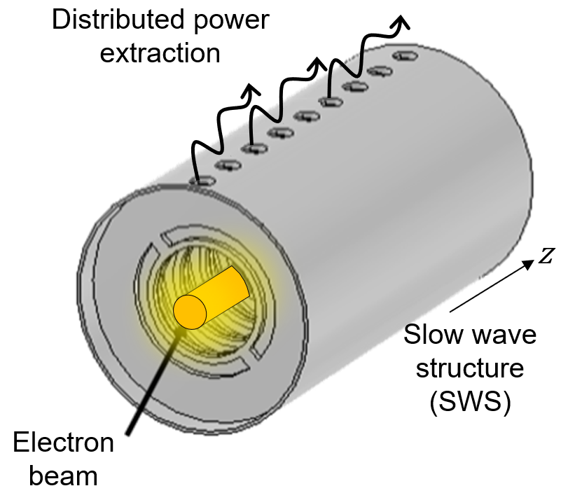
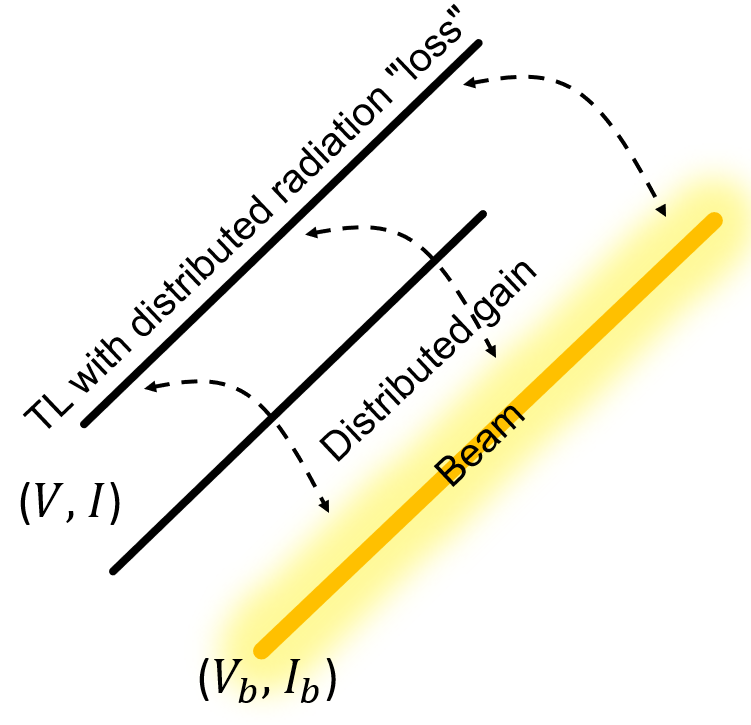
Figure 1: (a) An example of SWS with distributed radiating slots that extract power from the guided modes interacting with the electron beam. (b) Pierce-based equivalent transmission line model of the SWS with distributed “loss” (i.e., radiation) coupled to the charge wave modulating the electron beam. From the transmission line point of view, the interaction with the beam is seen as distributed gain.

Consider the SWS shown in Fig. 1(a) supporting a Floquet-Bloch mode whose slow wave spatial harmonic interacts with an electron beam, and radiates via a distributed set of slots (radiation occurs via a fast wave spatial harmonic, usually the so called “-1” harmonic). The configuration in Fig. 1(a) is given as a possible realization, though another one may consist in collecting the power exiting the interaction zone in a distributed fashion by an adjacent waveguide. We assume that the interaction between the SWS mode and the electron beam is modeled via the Pierce small-signal theory of traveling-wave tubes [15, 28, 29, 30, 16, 31, 32] that describes the evolution of the EM fields and electron beam dynamics assuming small signal modulation in the beam’s electron velocity and charge density. The beam electrons have average velocity and linear charge density $u_{0}$ and $\rho_{0}$, respectively. The electron beam has an average (dc) current $I_{0}=-\rho_{0}u_{0}$ and a dc (time-average) equivalent kinetic dc voltage $V_{0}=\tfrac{1}{2}u_{0}^{2}/\eta$ [23], [33], and $\eta=e/m=1.758820\text{$\times$}10^{11}$ C/Kg is the charge-to-mass ratio of the electron with charge equal to $-e$ and $m$ is its rest mass and $\rho_{0}$ is negative. The small signal modulation in electron beam velocity and charge density $u_{b}$ and $\rho_{b},$ respectively, form the so called “charge wave”. The linearized basic equations governing charge motion and continuity are written in their simplest form as [16]

$$\begin{array}[]{c}\partial_{t}u_{b}+u_{0}\partial_{z}u_{b}=-\eta e_{z},\\ \partial_{t}\rho_{b}=-\rho_{0}\partial_{z}u_{b}-u_{0}\partial_{z}\rho_{b},\end{array}$$ (1)

where $e_{z}$ is the electric field component in the $z$-direction of the EM mode in the SWS interacting with the electron beam, and the operator $\partial_{\sigma}$ indicates differentiation with respect to the variable $\sigma$. For convenience, we define the equivalent kinetic beam voltage and current as $v_{b}=u_{b}u_{0}/\eta$ and $i_{b}=u_{b}\rho_{0}+u_{0}\rho_{b}.$ Assuming an $e^{i\omega t}$ time dependence for monochromatic fields, the two equations in (1) are written in terms of the beam equivalent voltage and current in phasor domain as

$$\begin{array}[]{c}\partial_{z}V_{b}=-i\beta_{0}V_{b}-E_{z},\\ \partial_{z}I_{b}=-igV_{b}-i\beta_{0}I_{b},\end{array}$$ (2)

where $\beta_{0}=\omega/u_{0}$ is the beam’s equivalent propagation constant and $g=\tfrac{1}{2}I_{0}\beta_{0}/V_{0}$. Small fonts are used for the time-domain representation while capital ones are used for the phasor-domain representation. The details of the model used to describe the electron beam and its fundamental equations that describe the beam’s dynamics in space and time are given in Appendix A.

The EM mode propagating in the SWS is described by the equivalent transmission line in Fig. 1(b), with distributed per-unit-length series impedance $Z$ and shunt admittance $Y$, and equivalent voltage $V(z)$ and current $I(z)$ phasors that satisfy the telegrapher’s equations

$$\begin{array}[]{c}\partial_{z}V=-ZI,\\ \partial_{z}I=-YV+I_{s}.\end{array}$$ (3)

The term $I_{s}$ in (3) accounts for the electron stream flowing in the SWS that loads the TL as a shunt displacement current according to [16, 29, 32] and whose expression is given by $I_{s}=-\partial_{z}I_{b}$. For the non-interactive EM system (i.e., when $I_{s}$=0), the propagation constant and the characteristic impedance of the electromagnetic mode are given by $\beta_{p}=\sqrt{-ZY}$ and $Z_{c}=\sqrt{Z/Y}$, respectively. The two root solutions represent waves that propagate in opposite directions, i.e., both $\beta_{p}$ and $-\beta_{p}$ are valid solutions because of reciprocity. In this paper we consider that the SWS supports either a “forward” or a “backward” mode. The modal propagation constant is a complex number, $\beta_{p}=\beta_{pr}+i\beta_{pi},$where $\beta_{r}\beta_{i}<0$ for forward modes and $\beta_{r}\beta_{i}>0$ for backward modes. For example, when the the TL is supporting forward wave propagation both roots in $\beta_{p}$ and $Z_{c}$ must be taken as the principal square roots, so that their real part is positive. In this case $\beta_{p}$ turns out to be in in the fourth complex quadrant [34]. However, for TL supporting backward wave propagation the root of $\beta_{p}=\sqrt{-ZY}$ is taken as the principle square root (resulting in a positive real part) while the root of $Z_{c}=\sqrt{Z/Y}$ is taken as the secondary square root (resulting in a negative real part). In this case $\beta_{p}$ turns out to be in in the first complex quadrant[34].

Based on the Pierce’s model [16], the EM wave couples to the electron beam with its longitudinal electric field given by $E_{z}=-\partial_{z}V$. For convenience, we define a state vector $\mathbf{\boldsymbol{\Psi}}(z)=[\begin{array}[]{cccc}V(z),&I(z),&V_{b}(z),&I_{b}(z)\end{array}]^{T}$ that describes the system evolution with coordinate $z$. Thus, the interacting EM mode and electron-beam charge wave are described as [32]

$$\partial_{z}\mathbf{\boldsymbol{\Psi}}(z)=-i\mathbf{\underline{\mathbf{M}}}\mathbf{\boldsymbol{\Psi}}(z),$$ (4)

where $\mathbf{\underline{\mathbf{M}}}$ is the $4\times 4$ system matrix

$$\underline{\mathbf{M}}=\left[\begin{array}[]{cccc}0&-iZ&0&0\\ -iY&0&-g&-\beta_{0}\\ 0&-iZ&\beta_{0}&0\\ 0&0&g&\beta_{0}\end{array}\right].$$ (5)

This description in terms of a multidimensional first order differential equation in (4) is ideal for exploring the occurrence of EPDs in the system since an EPD is a degeneracy associated to two or more coalescing eigenmodes, hence it occurs when the system matrix $\underline{\mathbf{M}}$ is similar to a matrix that contains a non-trivial Jordan block. In general there are four independent eigenmodes, and each eigenmode is described by an eigenvector $\mathbf{\boldsymbol{\Psi}}(z)$, hence it includes both the EM and the charge wave. At the EPD investigated in this paper two of these four eigenvectors coalesce.

III Second order EPD in an interacting electromagnetic wave and an electron beam’s charge wave

Assuming a state vector z-dependence of the form $\boldsymbol{\Psi}(z)\propto e^{-ikz}$, where $k$ is the wavenumber of a mode in the interacting system, i.e., in the hot SWS, the eigenmodes are obtained by solving the eigenvalue problem $k\mathbf{\boldsymbol{\Psi}}(z)=\underline{\mathbf{M}}\mathbf{\boldsymbol{\Psi}}(z)$, and the modal dispersion relation is given by

$$\begin{array}[]{c}D(\omega,k)=\mathrm{det}\left(\mathbf{\underline{\mathbf{M}}}-k\mathbf{\underline{\mathbf{I}}}\right)\\ =k^{4}-2\beta_{0}k^{3}+\left(\beta_{0}^{2}+ZY-iZg\right)k^{2}\\ \ \ \ \ \ \ \ \ \ \ \ \ \ \ \ \ \ \ \ \ \ \ \ \ \ \ \ \ \ \ \ \ \ \ -2\beta_{0}ZYk+\beta_{0}^{2}ZY=0.\end{array}$$ (6)

The solution of this equation leads to four modal complex wavenumbers that describe the four modes in the EM-electron beam interactive system. A second order EPD occurs when two of these eigenmodes coalesce in their eigenvalues and eigenvectors, which means that the matrix $\underline{\mathbf{M}}$ is similar to a matrix that contains a Jordan block of order two [20, 21]. Following the theory in [35], the algebraic formulation that is often used to determine EPDs (and summarized in Appendix B) is equivalent to a bifurcation theory that is here applied. Indeed the EPD radian frequency and wavenumber are simply obtained by setting $D(\omega_{e},k_{e})=0$ and $\partial_{k}D(\omega_{e},k)\big{|}_{k_{e}}=0$ as in [35], where the EPD is designated with the subscript $e$. Based on the details provided in Appendix B these two conditions show that the EPD occurs when the transmission line per-unit-length series impedance and shunt admittance are $Z=Z_{e}$ and $Y=Y_{e}$, where

$$\begin{array}[]{ccc}Z_{e}=\dfrac{i\beta_{0e}^{2}\delta_{e}^{3}}{g_{e}},&&Y_{e}=\dfrac{ig_{e}(\delta_{e}+1)^{3}}{\delta_{e}^{3}},\end{array}$$ (7)

and $\delta_{e}=(k_{e}-\beta_{0e})/\beta_{0e}$ represents the relative deviation of degenerate modal wavenumber $k_{e}$ (of the interactive system) from the beam equivalent propagation constant $\beta_{0e}=\omega_{e}/u{}_{0}$.

Using (7), we constrain $\delta_{e}$ to provide $Z_{e}$ and $Y_{e}$ with positive real part, that means we assume that the TL is passive because of SWS losses and especially because of the distributed power extraction mechanism (see Appendix B). Figure 2 shows the two sectoral regions of $\delta_{e}$ that allow EPDs for transmission line that support either forward or backward propagation. These two regions satisfy the passivity condition of the TL, $\mathrm{Re}(Z)\geq 0$ and $\mathrm{Re}(Y)\geq 0$, where the real part of $Z$ and $Y$ represents mainly distributed power extraction (i.e., radiation losses using a terminology in the antennas community). It is important to point out that dark blue regions in Fig. 2 correspond to complex values of $\delta_{e}$ where EPD is obtained for TL that has also gain (independently of the electron beam). As explained in Appendix B, the two light blue and red narrow sectoral regions in Fig. 2 also correspond to an electron beam that delivers energy to the TL. In the rest of this paper we focus on the light blue region that represents complex values of $\delta_{e}$ associated to EPDs resulting from the interaction of a backward propagating electromagnetic wave and the charge wave modulating the electron beam. We stress that distributed radiated power is represented by series and/or parallel “losses” in the passive TL.

We now simplify the two equations given in (7) to get rid of $\delta_{e}$ as follows: from the first equation in (7) we find that $\delta_{e}=\sqrt[3]{-ig_{e}Z_{e}/\beta_{0e}^{2}}$, where the proper choice of root, based on chart in Fig. 2, is the one that guarantees the passivity of the TL and that there is power delivered from the beam to the TL (see Appendix B). For example, the root of $\sqrt[3]{-ig_{e}Z_{e}/\beta_{0e}^{2}}$ should lie in the light blue region in the chart to have an EPD with passive TL that support backward wave. Roots of $\sqrt[3]{-ig_{e}Z_{e}/\beta_{0e}^{2}}$ that lie in the dark blue region are ignored because they would result in an EPD that requires an active TL, while here we consider only passive TLs because of power extraction. The EPD conditions in (7) are simplified by substituting the previous expression of $\delta_{e}$ in the second equation of (7), leading to an interesting equation that constrains the TL parameters and the electron beam parameter $g_{e}$:

$$-Z_{e}Y_{e}/\beta_{0e}^{2}=\left(\sqrt[3]{-ig_{e}Z_{e}/\beta_{0e}^{2}}+1\right)^{3}.$$ (8)

The above equation constrains all the system parameters to have an EPD, hence it says that for an EPD to occur, a specific choice of the electron beam current $I_{0}=I_{0e}$ and angular frequency $\omega=\omega_{e}$ must be selected. In other words it says that for a given electron beam described by $\beta_{0e}$, and $g_{e}$, the cold TL parameters $Z_{e}$ and $Y_{e}$ must be chosen accordingly. The condition in (8 can also be rewritten in term of the propagation constant $\beta_{pe}$ and the characteristic impedance $Z_{ce}$ of the cold TL as $(\beta_{pe}/\beta_{0e})^{2}=\left(\sqrt[3]{g_{e}Z_{ce}\beta_{pe}/\beta_{0e}^{2}}+1\right)^{3}.$

In general, the interaction between the charge wave and the EM wave occurs when they are synchronized, i.e., by matching the EM wave phase velocity $\omega/\beta_{p}$ to the average velocity of the electrons $u_{0}=\omega/\beta_{0}$, a condition that is specifically called “synchronization”. Note that this is just an initial criterion, because the phase velocity of the modes in the interactive systems are different from $\omega/\beta_{p}$ and $u_{0}$. When the system parameters are such that equation (8) is satisfied and hence an EPD occurs, there are two modes (in the interactive system) that have exactly the same phase velocity $\omega/\mathrm{Re}(k_{e})$. Since this synchronization condition corresponds to an EPD, the two modes in the interactive system are actually identical also in their eigenvectors $\boldsymbol{\Psi}$. Note that the spatial z-evolution of the interacting EM and electron charge wave is described by four modes that are solutions of (4), three of which have a positive real part of $k$, as discussed next and in Appendix B. At the EPD two of these four modes coalesce, i.e., they become identical, that is why we refer to this condition as “degenerate synchronization”. In this paper we explore and enforce this very special kind of synchronization based on an EPD. In particular we enforce two of the resulting eigenmodes to fully coalesce in both their wavenumber and system state variable $\mathbf{\boldsymbol{\Psi}}(z)$. This condition is a new kind of EPD found in physical systems since it involves the coupling between two different media of propagation, and may be very promising for achieving new regimes of operation in electron beam devices with features not obtainable in conventional regimes.

The EPD condition obtained in (8) guarantees that the system has two repeated eigenvalues and two coalesced eigenvectors (see Appendix B)

$$\begin{array}[]{c}k_{e}=\sqrt[3]{\beta_{0e}\beta_{pe}^{2}},\\ \\ \mathbf{\Psi}_{e}=[\begin{array}[]{cccc}1,&ik_{e}/Z,&1/\delta_{e},&g_{e}/(\beta_{0e}\delta_{e}^{2})\end{array}]^{T},\end{array}$$ (9)

that form the “degenerate synchronization”. For the interacting system of EM and charge wave, the EPD represents a point in parameter space at which the system matrix $\mathbf{M}$ in (5) is not diagonalizable and it is indeed similar to a matrix that contains a $2\times 2$ Jordan block. This implies that the solution of (4) includes an algebraic linear growth factor resulting in unusual wave propagation characteristics as discussed next.

Solution of (6) leads to four eigenmode wavenumbers and due to the highly non-reciprocal physical nature of the electron beam, three have positive real part (i.e., $\mathrm{Re}(k)>0$) and one has it negative. According to the traveling-wave tube theory in [36], [16], conventionally applied to BWOs [22], these three distinct wavenumbers with $\mathrm{Re}(k)>0$ participate to the synchronization mechanism, and the electric field in the SWS is generally represented as

$$V(z)=V_{1}e^{-ik_{1}z}+V_{2}e^{-ik_{2}z}+V_{3}e^{-ik_{3}z}.$$ (10)

Remarkably, at the EPD the interactive system has two modes with the same degenerate wavenumber $k_{e}$, resulting in a guided electric field with linear growth factor as

$$V(z)=zV_{1}e^{-ik_{e}z}+V_{2}e^{-ik_{e}z}+V_{3}e^{-ik_{3}z}$$ (11)

which is completely different from any other regime of operation. A degenerate mode described by $\mathbf{\boldsymbol{\Psi}_{\mathit{e}}}$ is composed also of the charge wave, which implies that also the charge wave propagation is described as in (11), with two terms having the same degenerate wavenumber $k_{e}$, and one of them exhibiting the algebraic linear growth besides the exponential behavior.

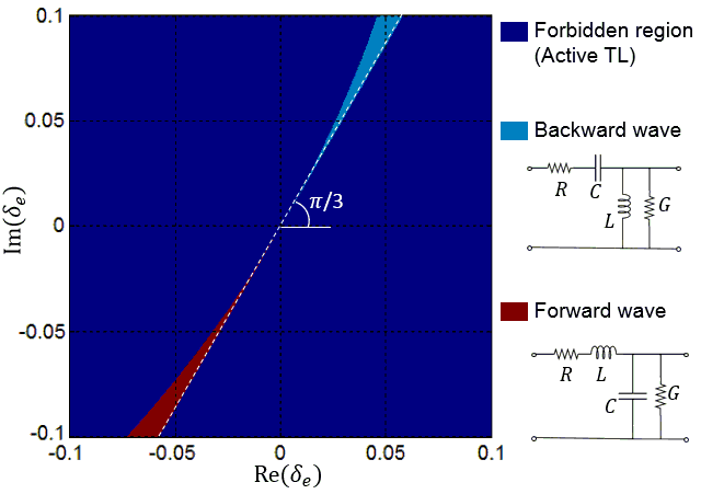
Figure 2: The two sectoral regions represent complex values of $\delta_{e}$, associated to EPDs resulting from the interaction of backward or forward electromagnetic waves (radiation is represented in TL by series or/and parallel losses) and the charge wave of electron beam. The value $\delta_{e}=(k_{e}-\beta_{0})/\beta_{0}$ represents the wavenumber deviation of the EPD complex wavenumber $k_{e}$ (of the interactive system) from the equivalent electron beam wavenumber $\beta_{0}$, that satisfies (7), assuming SWS realizations based on passive equivalent TLs. There are two regions of possible realizations (red and light blue), associated to the two distributed per-unit-length TL circuits on the right panel, that represent SWSs supporting either forward or backward wave propagation. In this paper we focus on EPDs obtained from backward electromagnetic waves interacting with an electron beam, i.e., those leading to $\mathrm{Re}(\delta_{e})>0$ and $\mathrm{Im}(\delta_{e})>0$.

In the following we show an example of degenerate synchronization based on an electron beam with dc voltage of $V_{0}=23$ kV and dc current of $I_{0}=0.1$ A. We derive the system parameters assuming that the EPD electron beam current $I_{0}=I_{0e}=0.1$ A (hence the choice of the TL parameters are chosen accordingly) and assume the operational frequency at which the EPD occurs is 1 GHz. We require (as an example) a relative degenerate wavenumber deviation of $\delta_{e}=0.01+i0.017$ that is lying exactly on the white dashed line shown in Fig. 2, with $\angle\delta_{e}=\pi/3$ (the phase of $\delta_{e}$). The corresponding wavenumber of two coalescing modes in the interactive system is $k_{e}=\left(1+\delta_{e}\right)\beta_{0e}$ which is $k_{e}=\left(1.01+i0.017\right)\beta_{0e}=70.55+i1.21$ $\mathrm{m}^{-1}$. By imposing the beam parameters and the chosen $\delta_{e}$ in the EPD conditions in (7) we obtain the distributed per-unit-length TL impedance and admittance of SWS to be $Z_{e}=-i257.1$ Ohm$\,\mathrm{m}^{-1}$ (i.e., capacitive) and $Y_{e}=1-i19.54$ Siemens$\,\mathrm{m}^{-1}$ (i.e., inductive with losses), representing a backward wave in the SWS. Losses here are not modeling energy damping but rather energy extraction (e.g., radiation) from the TL, per unit length, like in a backward leaky wave antenna [37]. To obtain these values, we have chosen the per-unit-length TL parameters for backward wave propagation as $C=0.62$ pFm, $L=8.14$ pHm, $R=0$ Ohm$\,\mathrm{m}^{-1}$ and $G=1$ Siemens$\,\mathrm{m}^{-1}$. Figure 3(a) shows the dispersion relation of three complex modes in the “hot” SWS, i.e., in the interactive EM wave-electron beam system, obtained using the Pierce model as explained in [32]. (The fourth mode with $\mathrm{Re}(k_{e})<0$ is not shown since it does not have a significant role in the synchronism). We show the real and imaginary parts of wavenumbers of three eigenmodes in the hot SWS versus normalized frequency (red curves), together with the dispersion of the beam alone (i.e., the beam “line” in green that actually represents two curves since we are neglecting the effect of the beam plasma frequency here) and of the backward wave in the cold SWS (blue curve, with negative slope). It is obvious from the figure that two eigenmodes of the interactive system coalesce at the EPD frequency $f_{e}$, forming an EPD of order two. Each of these two eigenmode has an EM wave and a charge wave counterpart, though far from the EPD frequency they tend to recover the beam line (green line) and the EM mode in the cold SWS (blue line).

We recall that the SWS is a periodic structure, and it is the slow wave harmonic of a mode that interacts with the electron beam charge wave. Though slow waves do not radiate, a spatial Floquet-Bloch harmonic of the mode is fast and able to radiate through the slots [37], justifying the presence of the conductance $G=1$ Siemens$\,\mathrm{m}^{-1}$, real part of $Y_{e}=1-i19.54$ Siemens$\,\mathrm{m}^{-1}$, in the TL model.

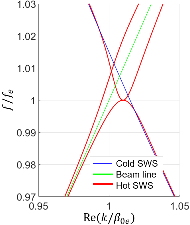
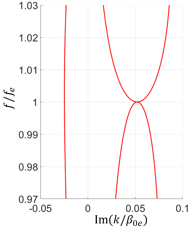
Figure 3: Dispersion diagram for three of the four complex modes in the “hot” SWS (the modes in the SWS interacting with the electron beam), in red, showing the existence of a second order EPD, where two modes coalesce in their wavenumbers and eigenvectors: (a) Real part of the wavenumber of the modes phase-propagating in the positive $z$ direction ($\mathrm{Re}(k_{e})>0$). The blue line represents the dispersion of the EM mode in the cold SWS supporting a backward propagation, whereas the green line is the electron beam’s charge wave dispersion, without accounting for their interaction. (b) Imaginary part of the wavenumber of the three modes with $\mathrm{Re}(k_{e})>0$ resulting from the interaction. The EPD wavenumber at $f=f_{e}$ represents two fully degenerate and synchronous modes with exponential growth in z.

IV EPD-BWO threshold current

The EPD is here employed to conceive a new regime of operation for BWOs based on “degenerate synchronization” between an EM wave and the electron beam. To explain this concept we refer to the setup in Fig. 4(a) for a BWO that has “balanced gain and radiation-loss” per unit length, where distributed loss is actually representing distributed radiation (per unit length) via a shunt conductance $G$ (see Fig. 4). The description is following the steps in [16] and [22] outlined for BWOs, where the TL is represented by a distributed circuit model shown in Fig. 4(b) that supports backward waves. An important difference from a standard BWO is that here the TL has shunt distributed “losses” that actually model the distributed radiation and whose presence is necessary to satisfy the EPD condition (8). We assume to have an unmodulated space charge at the beginning of the electron beam, i.e., $V_{b}(z=0)=0$ and $I_{b}(z=0)=0$ and we assume that the SWS waveguide length is $\ell=N\lambda_{e}$, where $\lambda_{e}=2\pi/\beta_{0e}$ is the guided wavelength calculated at the EPD frequency and N is the normalized SWS length. We also assume that the SWS waveguide is terminated by a load at $z=0$ matched to the characteristic impedance of the TL (without loss and gain) $R_{o}=\sqrt{L/C}$ and by a short circuit at $z=\ell$. We follow the same procedure used in [22] to obtain the starting oscillation condition which is based on imposing infinite voltage gain $A_{v}=V(0)/V(\ell)\to\infty$ . After simplification, and using the three-wave traveling-wave theory [16, 22], the voltage gain is written in terms of the three modes concurring to the synchronization (those with $\mathrm{Re}(k)>0$ ) as

$$\begin{array}[]{c}A_{v}^{-1}e^{i\beta_{0}\ell}=\dfrac{e^{-i\beta_{0}\delta_{1}\ell}\delta_{1}^{2}}{\left(\delta_{1}-\delta_{2}\right)\left(\delta_{1}-\delta_{3}\right)}+\dfrac{e^{-i\beta\delta_{2}\ell}\delta_{2}^{2}}{\left(\delta_{2}-\delta_{3}\right)\left(\delta_{2}-\delta_{1}\right)}\\ \\ \ \ \ \ \ \ \ \ \ \ \ \ \ \ \ \ \ \ \ \ \ \ \ \ \ \ \ \ \ \ \ \ \ \ \ \ \ \ \ +\dfrac{e^{-i\beta_{0}\delta_{3}\ell}\delta_{3}^{2}}{\left(\delta_{3}-\delta_{1}\right)\left(\delta_{3}-\delta_{2}\right)}=0,\end{array}$$ (12)

where $\delta_{n}=(k_{n}-\beta_{0})/\beta_{0}$ and $k_{1},k_{2}$ and $k_{3}$ are the three wavenumbers of the interactive EM-beam system with positive real part that are solutions of (6). In close proximity of the EPD there are two modes coalescing, with $\delta_{1}=\delta_{a}+\Delta/2$ and $\delta_{2}=\delta_{a}-\Delta/2$ where $\delta_{a}=(\delta_{1}+\delta_{2})/2$ is the average, and $|\Delta|\ll|\delta_{a}|$ is a very small quantity that vanishes at the EPD. By observing that $|e^{-i\beta_{0}\delta_{3}\ell}|\ll 1$ for very large $\ell$ because Im($k_{3}$)<0, the gain expression in (12) reduces to

$$\begin{array}[]{c}A_{ve}^{-1}e^{i\beta_{0}\ell}\approx\dfrac{e^{-i\beta_{0}\delta_{a}\ell}\delta_{a}^{2}}{\left(\delta_{a}-\delta_{3}\right)}\dfrac{\sin\left(\Delta\beta_{0}\ell/2\right)}{\Delta/2}=0\end{array}.$$ (13)

From the above condition, assuming very large $\ell$, the first oscillation frequency occurs when $\Delta\beta_{0}\ell=2\pi$. This happens when the constraint on the wavenumbers $k_{1}-k_{2}=2\pi/\ell$ is satisfied. This shows a very important fact, that for infinitely long structure $\ell\to\infty$ the starting oscillation condition is $k_{1}=k_{2}=k_{e}$, which corresponds to the EPD condition. This implies that the EPD is the exact condition for synchronization between the charge wave and EM wave, accounting for the interaction in infinitely long SWSs, that guarantees the generation of oscillations at the EPD frequency $f_{e}=\omega_{e}/(2\pi)$.

For finite length SWS, oscillations occurs when $k_{1}-k_{2}=2\pi/\ell$ is satisfied, assuming very large $\ell$, and since $|\Delta|\ll|\delta_{a}|$, we have both $k_{1}$ and $k_{2}$ very close to $k_{e}$, which implies that the systems is close to the EPD and hence the threshold beam current $I_{th}$ that starts oscillations is slightly different from $I_{0e}$. A beam current slightly away from the EPD one causes the wavenumbers to bifurcate from the degenerate one $k_{e}$, following the Puiseux series approximation [38] (also called fractional power expansion) as

$$k_{n}-k_{e}\approx(-1)^{n}\alpha\sqrt{I_{0}-I_{0e}},$$ (14)

with $n=1,2$ , and $\alpha$ is a constant. This implies that $k_{1}-k_{2}\approx-2\alpha\sqrt{I_{0}-I_{0e}}$, and by comparing this with the $k_{1}-k_{2}$ difference associated to the threshold beam current in a finite length SWS we infer that the threshold beam current $I_{th}$ that makes the EPD-BWO of finite length $\ell$ oscillate, asymptotically scales as

$$I_{th}\sim I_{0e}+\left(\dfrac{\pi/\alpha}{\ell}\right)^{2}.$$ (15)

In a conventional BWO, that has no distributed power extraction and the power is delivered only to the load $R_{0}$, the threshold current scaling decrease with the SWS length asymptotically as $I_{th}\sim\zeta/\ell^{3}$ [39, 22], where $\zeta$ is a constant. Instead, the EPD-BWO has a threshold current in (15) always larger than the EPD beam current $I_{0e}$, which represents the current that keeps the oscillation going and simultaneously balance the distributed radiated power. Importantly, the EPD beam current $I_{0e}$ can be engineered to any desired (high) value depending on how much power one wants to extract from the electron beam.

The above derivation was based on assuming $\ell\to\infty$ (details are in Appendix D), and a rigorous derivation for any EPD-BWO length is shown in Appendix C that leads to the determination of the threshold current and oscillation frequency. This formulation based on the Pierce model for the beam current threshold is used to compute the results shown in Fig. 4 for varying the EPD-BWO length and the shunt conductance G that represents the distributed radiation.

Figure 4(c) shows the scaling of the threshold current versus SWS length for a system with the same parameters used in the previous example. The scaling shows that for infinitely long SWSs the oscillation starting current is equal to the EPD beam current $I_{0e}$ which is consistent with the asymptotic relation in (15). Figure 4(d) also shows a comparison between the threshold current of the conventional BWO (that does not have distributed power extraction, i.e., $G=0$) and that of the EPD-BWO (with distributed power extraction, represented by $G=1$ Siemens$\,\mathrm{m}^{-1}$) by showing their current scaling with the SWS length. The threshold beam current $I_{th}$ of the conventional BWO vanishes when the SWS length increases, whereas the threshold beam current $I_{th}$ of the EPD-BWO tends to the value of $I_{0e}=0.1$ A. Figure 4(e) shows the threshold beam current $I_{0}=I_{0e}$ (blue curve) that leads to the EPDs as a function of the radiation “loss” per unit length G . We also show the required starting beam current (i.e. the threshold) for oscillations (red curve) for a finite length “hot” SWS working at the EPD; we assume the SWS length normalized to the wavelength at the EPD frequency of $N=70$. It is important to point out that the radiated power per-unit-length of the SWS is determined using $p_{rad}(z)=\tfrac{1}{2}G|V(z)|^{2}$, thus it is linearly proportional to the parameter $G$ , i.e., higher values of $G$ imply higher radiated power per-unit-length and therefore higher level of energy extraction from the SWS.

We have shown two very important facts here: first, the threshold beam current is very close to the EPD beam current for any desired value of power extracted. This indicates that the EPD condition for hot SWSs with finite length is the condition that basically guarantees full synchronization between the EM guided mode and the beam’s charge wave. Secondly, the threshold current increases monotonically when increasing the required radiated power per unit length which implies a tight synchronization regime guaranteed for any high power generation. Therefore in principle the synchronism is maintained for any desired power output, according to the Pierce model, and this trend is definitely not observed in standard backward wave oscillators where the load is at the beginning of the SWS.

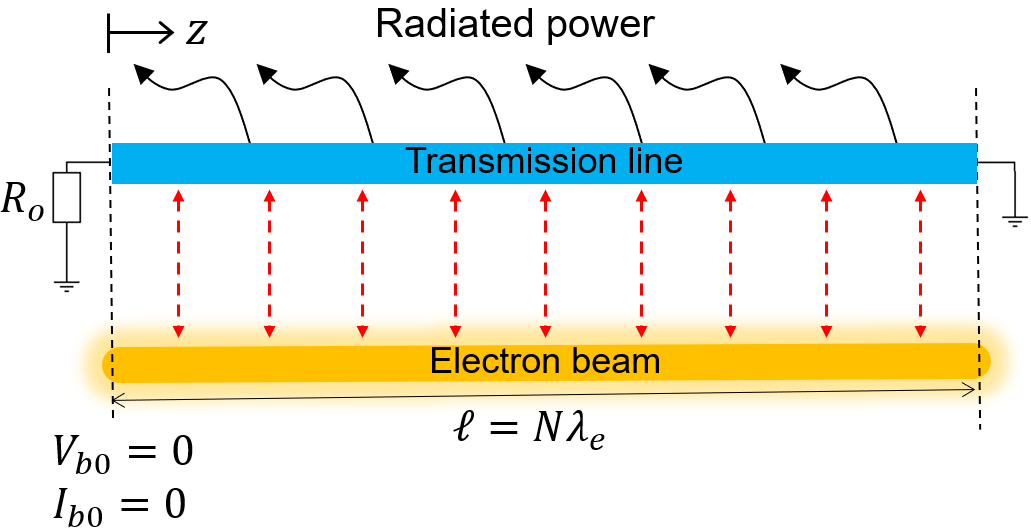
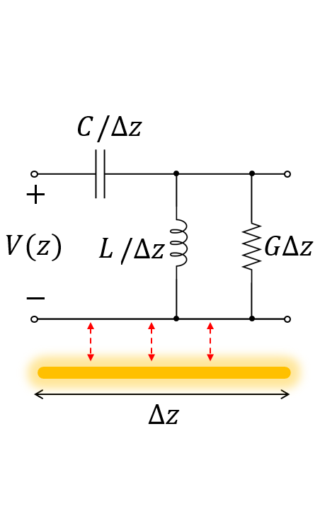
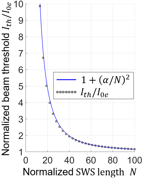
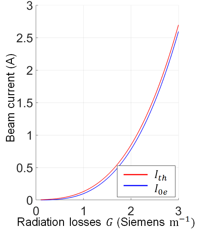
Figure 4: (a) Schematic setup for BWOs with “balanced gain and radiation-loss”. (b) Equivalent transmission line model of the SWS with distributed (per-unit-length) series capacitance and shunt inductance for a SWS that supports backward waves. The distributed shunt conductance G represents distributed power extraction, that is indeed given by $p_{rad}(z)=G|V(z)|^{2}/2$. (c) Scaling of the oscillation-threshold beam current $I_{th}$ versus SWS length normalized to the wavelength $N=\ell/\lambda_{e}$, where $\lambda_{e}=2\pi/\beta_{0e}$ is the guided wavelength calculated at the EPD frequency. It is obvious that for infinite long SWS where $N\rightarrow\infty$ we have $I_{th}\rightarrow I_{0e}$ which implies that the EPD synchronization condition is also the threshold for infinitely long SWSs. (d) Comparison of the threshold current for an EPD-BWO and a standard BWO for increasing SWS length. Note that the threshold of the EPD-BWO does not decreases to zero for longer SWSs, a characteristic that is fundamentally different from that of a standard BWO. (e) Scaling of the EPD beam current $I_{0}=I_{0e}$ (blue curve) versus radiation losses $G$. We also show the scaling of the threshold beam current (red curve) for a finite-length SWS with $N=70$. Note that the threshold beam current is very close to the EPD current for any amount of required distributed extracted power which indicates that in principle the synchronism is achieved for any output power level.

V Conclusion

We have conceptually demonstrated the occurrence of an EPD in an interactive system made of a linear electron beam and a guided electromagnetic wave. This EPD condition leads to a new regime of operation for BWOs where the EPD guarantees a synchronism between a backward wave and a beam’s charge wave through enforcing the coalescence of two modes in both their wavenumber and state vector, a regime we named “degenerate synchronization”. A remarkable aspect of this EPD-BWO regime is that the “gain and distributed-power-extraction balance” condition leads to a perfect degenerate synchronization between the charge wave and EM wave for any amount of designed distributed power extraction. This distributed power extraction can be in the form of distributed radiation from the interaction zone or of distributed transfer of power from the hot SWS to an adjacent coupled waveguide. Under this EPD-BWO regime, in principle it is possible to extract large amounts of power from the electron beam and therefore the EPD-BWO exhibits high starting beam current. In theory the starting-oscillation beam current (i.e, the threshold) could be set to arbitrary large values, in contrast to what happens in conventional BWOs where the beam’s starting current tends to vanish when the SWS lengths increases. Remarkably, in the EPD-BWO regime the starting oscillation current is always larger than the EPD’s beam current that, in principle, can be set to large values by increasing the amount of power extracted per unit length. Therefore we have shown the fundamental principle that the amount of power generated under the EPD-BWO regime has no upper limit (the actual limit would be imposed only by the constraints encountered in the practical realizability), contrarily to conventional knowledge of BWOs.

Note that the degenerate synchronization regime discussed in this paper is very different from the ones discussed in [24, 25, 26, 27]. There, it was the “cold” SWS that exhibited a degeneracy condition, like the degenerate band edge (DBE), which is an EPD of order four, or the stationary inflection point (SIP), which is an EPD of order three, that were proposed to enhance the performance of high power devices. Those DBE and SIP EPD conditions were obtained in "cold" SWSs based on periodicity, and indeed the interaction of the EM modes with the electron beam would perturb those degeneracy conditions, and even destroy them for increasingly large values of electron beam currents. Here, instead, we have proposed a new fully synchronous degenerate regime based on the concept of “distributed radiation and gain balance”, where the EPD occurs in the "hot" structure, i.e., in presence of the interacting electron beam with any amount of current and hence, in principle, for any large amount of power.

VI Acknowledgment

This material is based upon work supported by the Air Force Office of Scientific Research award number FA9550-18-1-0355.

Appendix A Electron beam model

We show the fundamental equations that describe the evolution of electron beam dynamics in space and time. We follow the linearized equations that describe the space-charge wave on the electron beam presented in Pierce[16] based on the electron beam model in [15]. We assume a narrow cylindrical beam of electrons subject to axial electric field that is constant across the beam’s cross section; we assume purely longitudinal electron motion as conventionally done in many electron beam devices thanks to confinement due to applied magnetic field, and negligible repulsion forces between electrons (hence we neglect space charge’s induced forces) compared to the force induced by the longitudinal electric field associated to the radio frequency mode in the slow wave structure (SWS) (this last assumption could be easily removed). The beam’s total linear-charge density and electron speed are represented as

$$\begin{array}[]{c}\rho(z,t)=\rho_{0}+\rho_{b}\\ u(z,t)=u_{0}+u_{b},\end{array}$$ (16)

where the subscripts ’$0$’ and ’$b$’ denote dc (average value) and ac (alternate current, i.e., modulation), respectively, and $\rho_{0}$ here is negative and $u$ is the electron speed in the $z$-direction. The basic equations governing the charges’ motion and continuity are written in their simplest form as [16]

$$\begin{array}[]{c}\dfrac{du}{dt}=-\eta e_{z}\\ \dfrac{\text{$\partial$}\rho}{\text{$\partial$}t}=-\dfrac{\text{$\partial$}(\rho u)}{\text{$\partial$}z}\end{array}$$ (17)

where $\eta=e/m=1.758820\text{$\times$}10^{11}$ C/Kg is the charge-to-mass ratio of the electron such that the electron charge is equal to $-e$ and $m$ is its rest mass. Assuming small signal modulation [29, 15], $|u_{b}|\ll u_{0}$ and $|\rho_{b}|\ll|\rho_{0}$|, (17) is linearized to

$$\begin{array}[]{c}\dfrac{\partial u_{b}}{\partial t}+u_{0}\dfrac{\text{$\partial$}u_{b}}{\text{$\partial$}z}=-\eta e_{z}\\ \text{$\dfrac{\text{$\partial$}\rho_{b}}{\text{$\partial$}t}$}=-\rho_{0}\dfrac{\partial u_{b}}{\partial z}-u_{0}\dfrac{\partial\rho_{b}}{\partial z}\end{array}$$ (18)

For convenience, we define the equivalent kinetic beam voltage and current [16] as

$$\begin{array}[]{c}v(z,t)=\dfrac{u^{2}}{2\eta}=V_{0}+v_{b},\\ i(z,t)=u\rho=-I_{0}+i_{b}.\end{array}$$ (19)

Again, assuming small signal modulation [29, 15], $|u_{b}|\ll u_{0}$ and $|\rho_{b}|\ll\rho_{0}$, we neglect the terms $u_{b}^{2}$ and $u_{b}\rho_{b}$ in (19). Thus, the dc and ac beam voltage and current are determined as a function of the dc and ac beam charge density and speed [23], [33], [16] as

$$\begin{array}[]{c}V_{0}=\tfrac{1}{2}u_{0}^{2}/\eta,\\ I_{0}=-\rho_{0}u_{0},\\ v_{b}=u_{b}u_{0}/\eta,\\ i_{b}=u_{b}\rho_{0}+u_{0}\rho_{b}.\end{array}$$ (20)

By substituting (20) into (18), the evolution equations of beam equivalent kinetic voltage and current are written as

$$\begin{array}[]{c}\dfrac{\text{$\partial$}v_{b}}{\text{$\partial$}z}=-\dfrac{1}{u_{0}}\dfrac{\text{$\partial$}v_{b}}{\text{$\partial$}t}-e_{z},\\ \dfrac{\text{$\partial$}i_{b}}{\text{$\partial$}z}=\dfrac{\eta\rho_{0}}{u_{0}^{2}}\dfrac{\text{$\partial$}v_{b}}{\text{$\partial$}t}-\dfrac{1}{u_{0}}\dfrac{\text{$\partial$}i_{b}}{\text{$\partial$}t}.\end{array}$$ (21)

Assuming time-harmonic signals with time convention $e^{i\omega t}$, that is omitted in the following for simplicity, equations in (21) are simplified to

$$\begin{array}[]{c}\dfrac{\text{$\partial$}V_{b}}{\text{$\partial$}z}=\dfrac{-i\omega}{u_{0}}V_{b}-E_{z},\\ \dfrac{\text{$\partial$}I_{b}}{\text{$\partial$}z}=\dfrac{i\omega\eta\rho_{0}}{u_{0}^{2}}V_{b}-\dfrac{i\omega}{u_{0}}I_{b}.\end{array}$$ (22)

When the electron beam is not interacting with an electromagnetic wave, i.e., when $E_{z}=0$, the charge wave has propagation constant $\beta_{0}=\omega/u_{0}$.

Appendix B Second order EPD in a system made of an electromagnetic wave interacting with an electron beam charge’s wave

The solution of the dispersion equation in Eq. (6) has four roots which represent the eigenvalues of the interactive system composed of guided EM waves and the charge waves that modulate the electron beam. A necessary condition to have second order EPD is to have two repeated eigenvalues, which means that the characteristic equation should have two repeated roots as

$$\begin{array}[]{c}D(\omega_{e},k)\propto(k-k_{e})^{2}\end{array}$$ (23)

where $\omega_{e}$ and $k_{e}$ are the degenerate angular frequency and wavenumber, respectively. The relation in (23), that guarantees having two coalescing waenumbers, is satisfied when [35]

$$\begin{array}[]{c}D(\omega_{e},k_{e})=0,\\ \dfrac{\partial D(\omega_{e},k)}{\partial k}\Bigg{|}_{k=k_{e}}=0.\end{array}$$ (24)

Substituting the determinant expresion (6) into (24), the two EPD conditions are

$$\begin{array}[]{c}k_{e}^{4}-2\beta_{0e}k_{e}^{3}+\left(\beta_{0e}^{2}+Z_{e}Y_{e}-ig_{e}Z_{e}\right)k_{e}^{2}\\ \ \ \ \ \ \ \ \ \ \ \ \ \ \ \ \ \ \ \ \ \ \ \ \ \ -2\beta_{0e}Z_{e}Y_{e}k_{e}+\beta_{0e}^{2}Z_{e}Y_{e}=0,\end{array}$$ (25)

$$4k_{e}^{3}-6\beta_{0e}k_{e}^{2}+2\left(\beta_{0e}^{2}+Z_{e}Y_{e}-ig_{e}Z_{e}\right)k_{e}-2\beta_{0e}Z_{e}Y_{e}=0,$$ (26)

where the EPD is designated with the subscript $e$, i.e., the parameters with the subscript $e$ are calculated at the EPD frequency; for example, $\beta_{0e}=\omega_{e}/u_{0}.$ Only at a specific frequency (the EPD frequency) it is possible to find two identical eigenvalues. Therefore the above equation provides both the EPD radian frequency $\omega_{e}$ and wavenumber $k_{e}$.

The combination of the TL distributed series impedance $Z=Z_{e}$ and shunt admittance $Y=Y_{e}$ that provide the EPD are determined after making some mathematical manipulations in the two conditions in (25) and (26). First, we use (25) to get $Y_{e}$ in term of $Z_{e}$ and other system parameters as

$$Y_{e}=\dfrac{ig_{e}k_{e}^{2}}{\left(k_{e}-\beta_{0e}\right)^{2}}-\dfrac{k_{e}^{2}}{Z_{e}},$$ (27)

then we substitute this relation in (26) and solve for $Z_{e}$ which is found to be

$$Z_{e}=\dfrac{i\left(k_{e}-\beta_{0e}\right)^{3}}{\beta_{0e}g_{e}}.$$ (28)

We finally substitute $Z_{e}$ in (27) to obtain $Y_{e}$

$$Y_{e}=\dfrac{ig_{e}k_{e}^{3}}{\left(k_{e}-\beta_{0e}\right)^{3}}.$$ (29)

These two latter expressions are then rewritten as in (7). Assuming that the EPD conditions in (28) and (29) are satisfied, the degenerate wave number $k_{e}$ is determined by the product of (28) and (29) $Z_{e}Y_{e}=-k_{e}^{3}/\beta_{0e}$ and by recalling that $Z_{e}Y_{e}=-\beta_{pe}^{2}$ , leading to $k_{e}=\sqrt[3]{\beta_{0e}\beta_{pe}^{2}}$, which is the result in (9).

The eigenvectors $\mathbf{\mathbf{\Psi}}_{n}$ of the system are determined by solving

$$\left(\mathbf{\underline{\mathbf{M}}}-k_{n}\mathbf{I}\right)\mathbf{\mathbf{\Psi}_{\mathrm{\mathit{n}}}}=\mathrm{\mathbf{0},}$$ (30)

where $k_{n}$ with $n=1,2,3,4$ are the modal wavenumbers, and they are determined from (6). By solving (30), the eigenvectors are written in the form (each element of the eigenvector carries an implicit unit of Volt besides the units of the explicit parameters)

$$\mathbf{\mathbf{\Psi}_{\mathrm{\mathit{n}}}}=[\begin{array}[]{cccc}1,&ik_{n}/Z,&(1+\delta_{n})/\delta_{n},&g(1+\delta_{n})/(\beta_{0}\delta_{n}^{2})\end{array}]^{T},$$ (31)

where $\delta_{n}=(k_{n}-\beta_{0})/\beta_{0}$. As shown in [16], three of these four modes are strongly affected by the synchronization of the electron beam and the EM mode with positive phase velocity. Assuming that these three wavenumbers of the beam-EM mode interactive system are a slight perturbation of the unperturbed beam’s propagation constant, i.e, $k_{n}\approx\beta_{0}$ with, $n=1,2,3$ the eigenvector expression in (31) is approximated

$$\mathbf{\mathbf{\Psi}_{\mathrm{\mathit{n}}}}\approx[\begin{array}[]{cccc}1,&ik_{n}/Z,&1/\delta_{n},&g/(\beta_{0}\delta_{n}^{2})\end{array}]^{T}.$$ (32)

It is worth mentioning that the eigenvector expression in (31) is valid for any of the four modes of the interacting system. Whereas the expression in (32) is only valid for the three modes with positive $\mathrm{Re}(k)$, namely, for the three synchronous modes resulting from the interaction of the SWS EM mode with the electron beam. Those three synchronous modes are such that $k_{n}\approx\beta_{0}$ based on synchronization. Two of these eigenvectors coalesce at the EPD, forming the degenerate syncrhosim between the two modes $\mathbf{\mathbf{\Psi}}_{1}=\mathbf{\mathbf{\Psi}}_{2}=\mathbf{\mathbf{\Psi}}_{e}$, where

$$\mathbf{\Psi}_{e}\approx[\begin{array}[]{cccc}1,&ik_{e}/Z,&1/\delta_{e},&g_{e}/(\beta_{0e}\delta_{e}^{2})\end{array}]^{T}.$$ (33)

In summary, the two conditions in (7) represent constraints on the TL parameters, calculated at EPD frequency, that provide the second order EPD, where two eigenmodes of the interacting system have identical eigenvalues $k_{1}=k_{2}=k_{e}$ and eigenvectors $\mathbf{\mathbf{\Psi}}_{1}=\mathbf{\mathbf{\Psi}}_{2}=\mathbf{\mathbf{\Psi}}_{e}$. These two eigenmodes form the degenerate synchronization.

From the transmission line point of view the electron beam is modeled as parallel per-unit-length admittance

$$Y_{b}=\dfrac{-igk^{2}}{(k-\beta_{0})^{2}},$$ (34)

that loads the line [32]. For proper operation of this new degenerate BWO regime the TL should outcouple power in a distributed fashion and the electron beam should supply power to balance the power extraction in order to have a sustainable oscillation. This means that both the TL parameters $Z$ and $Y$ should be passive, i.e., $\mathrm{Re}(Z)>0$ and $\mathrm{Re}(Y)>0,$ and the beam equivalent admittance should be active, i.e., $\mathrm{Re}(Y_{b})<0$. These constraints are plotted in Fig. 5 as a function of the complex wavenumber deviation $\delta_{e}=(k_{e}-\beta_{0e})/\beta_{0e}$. The intersection of these three conditions on $\mathrm{Re}(Z)>0$ and $\mathrm{Re}(Y)>,$ and $\mathrm{Re}(Y_{b})<0$ lead to the realizability diagram in Fig. 5(d) which is the same as in Fig. 2.

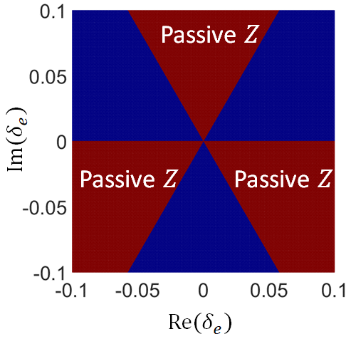
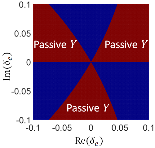
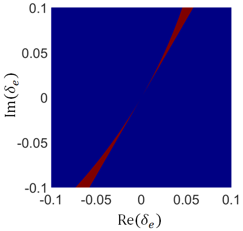
Figure 5: Regions of complex values $\delta_{e}$ that result in having passive TL, with $\mathrm{Re}(Z)>0$ and $\mathrm{Re}(Y)>0$ when EPD conditions are satisfied, i.e., when$Z=Z_{e}$ and $Y=Y_{e}$: (a) passive series impedance $\mathrm{Re}(Z_{e})=\mathrm{Re}(i\beta_{0e}^{2}\delta_{e}^{3}/g_{e})>0$ and (b) passive parallel admittance $\mathrm{Re}(Y_{e})=\mathrm{Re}(ig_{e}(\delta_{e}+1)^{3}/\delta_{e}^{3})>0$. (c) Regions of complex values $\delta_{e}$ where the electron beam delivers energy to the TL, i.e., when the electron beam provides gain from TL perspective, which means that $\mathrm{Re}(Y_{be})<0$, i.e., $\mathrm{Re}(-ig(1+\delta_{e})^{2}/\delta_{e}^{2})<0$. (d) Regions satisfying all the (a), (b) and (c) realizability criteria.

Appendix C Backward wave oscillator (BWO) threshold current

For a finite SWS with length $\ell$, the equivalent voltage that describes the electric field at any coordinate $z$ in the SWS is expanded as a combination of the four modes supported by the interactive beam-EM mode system (modes are calculated in a SWS of infinite length) as

$$V(z)=V_{1}e^{-ik_{1}z}+V_{2}e^{-ik_{2}z}+V_{3}e^{-ik_{3}z}+V_{4}e^{-ik_{4}z}$$ (35)

where $k_{n}$ with $n=1,2,3,4$ are the modes’ wavenumber, and they are determined from (6), and $V_{n}$ are the complex modes amplitudes. The associated TL current and beam dynamics are found by using (35) in (4) or by using the eigenvector expression in (31)

$$\begin{array}[]{c}I(z)=\dfrac{ik_{1}V_{1}}{Z}e^{-ik_{1}z}+\dfrac{ik_{2}V_{2}}{Z}e^{-ik_{2}z}\\ \ \ \ \ \ \ \ \ \ \ \ \ \ \ \ \ \ \ \ \ \ +\dfrac{ik_{3}V_{3}}{Z}e^{-ik_{3}z}+\dfrac{ik_{4}V_{4}}{Z}e^{-ik_{4}z},\\ \\ V_{b}(z)=\dfrac{(1+\delta_{1})V_{1}}{\delta_{1}}e^{-ik_{1}z}+\dfrac{(1+\delta_{2})V_{2}}{\delta_{2}}e^{-ik_{2}z}\\ \ \ \ \ \ \ \ \ \ \ +\dfrac{(1+\delta_{3})V_{3}}{\delta_{3}}e^{-ik_{3}z}+\dfrac{(1+\delta_{4})V_{4}}{\delta_{4}}e^{-ik_{4}z},\\ \\ I_{b}(z)=\dfrac{g(1+\delta_{1})V_{1}}{\beta_{0}\delta_{1}^{2}}e^{-ik_{1}z}+\dfrac{g(1+\delta_{2})V_{2}}{\beta_{0}\delta_{2}^{2}}e^{-ik_{2}z}\\ \ \ \ \ \ \ \ \ \ \ \dfrac{g(1+\delta_{3})V_{3}}{\beta_{0}\delta_{3}^{2}}e^{-ik_{3}z}+\dfrac{g(1+\delta_{4})V_{4}}{\beta_{0}\delta_{4}^{2}}e^{-ik_{4}z},\end{array}$$ (36)

where $\delta_{n}=(k_{n}-\beta_{0})/\beta_{0}.$ The setup we use for the BWO with distributed power radiation, shown in Fig. 4(a), is similar to that used in [22], where we assume unmodulated space charge at the beginning of the electron beam (i.e., $V_{b}(z=0)=0$ and $I_{b}(z=0)=0$), and we also assume that the output power is extracted at $z=0$, terminated with a resistance matched to the characteristic impedance of the TL (without loss and gain) $R_{o}=\sqrt{L/C}$, and short circuit at $z=\ell$, where $\ell=N\lambda_{e}$ is the SWS length (i.e the TL length), and $\lambda_{e}=2\pi/\beta_{0e}$ is the guided wavelength calculated at the EPD frequency. (Note that in the absence of loss and gain in the TL, the TL distributed series impedance and shunt admittance are $Z=1/(i\omega C)$ and $Y=1/(i\omega L)$). The boundary conditions that describe the mentioned setup are

$$\begin{array}[]{c}V(0)+R_{o}I(0)=0,\\ V(\ell)=0,\\ V_{b}(0)=0,\\ I_{b}(0)=0.\end{array}$$ (37)

By imposing (36) in (37), we obtain a homogeneous system of linear equations that is written in matrix form as

$$\mathbf{A}(\omega,I_{0})\mathbf{V}=\mathbf{0}$$ (38)

where $\mathbf{V}=[\begin{array}[]{cccc}V_{1},&V_{2},&V_{3},&V_{4}\end{array}]^{T}$. Free oscillation in the interactive system occurs when there is a solution of (38) despite the absence of the source term (the right hand side of (38) is equal to zero). Therefore, oscillation occurs for a combination of radian frequency and electron beam current that satisfy

$$\mathrm{det}(\mathbf{A}(\omega,I_{0}))=0.$$ (39)

Since the solution of the above equation defines the threshold beam current to start oscillations, such solution is denoted by $I_{0}=I_{th}$ and $\omega=\omega_{res}$ is the frequency of the oscillation.

Appendix D Asymptotic scaling of the EPD-BWO threshold beam current

In this section we derive the oscillation condition and the asymptotic scaling of the threshold beam current with the SWS length for the proposed EPD-BWO assuming that the length of the structure tends to infinity. We follow the traveling-wave tube theory used in [36], [16] and [22], since the synchronization involves mainly three waves, those with $Re(k_{n})>0$. Assuming that these three wavenumbers have a slight variation of the unperturbed beam wavenumber, i.e, $k_{n}\approx\beta_{0}$, we use the eigenvector expression in (32) to write the TL circuit voltage and beam dynamics distribution along the $z$-direction which are represented in terms of three modes as [22]

$$\begin{array}[]{c}V(z)=V_{1}e^{-ik_{1}z}+V_{2}e^{-ik_{2}z}+V_{3}e^{-ik_{3}z},\\ V_{b}(z)=\dfrac{V_{1}}{\delta_{1}}e^{-ik_{1}z}+\dfrac{V_{2}}{\delta_{2}}e^{-ik_{2}z}+\dfrac{V_{3}}{\delta_{3}}e^{-ik_{3}z},\\ I_{b}(z)=\dfrac{gV_{1}}{\beta_{0}\delta_{1}^{2}}e^{-ik_{1}z}+\dfrac{gV_{2}}{\beta_{0}\delta_{2}^{2}}e^{-ik_{2}z}+\dfrac{gV_{3}}{\beta_{0}\delta_{3}^{2}}e^{-ik_{3}z},\end{array}$$ (40)

where $\delta_{n}=(k_{n}-\beta_{0})/\beta_{0}$. The wavenumbers $k_{n}$ with $n=1,2,3$ are with positive real part and two of them are with positive imaginary part, let’s say $n=1,2$ and the other one is with negative imaginary part, $n=3$. A numerical example of the wavenumbers is shown in Fig. 3. Here, we follow the same procedure used in [22] to obtain the oscillation condition which is based on imposing infinite voltage gain $A_{v}=V(0)/V(\ell)\to\infty$ . By imposing the beam boundary condition $V_{b}(0)=0$ and $I_{b}(0)=0$ in (40) and after some mathematical manipulations the gain expression is written in its simplest form as [22]

$$\begin{array}[]{c}A_{v}^{-1}e^{i\beta_{0}\ell}=\dfrac{e^{-i\beta_{0}\delta_{1}\ell}\delta_{1}^{2}}{\left(\delta_{1}-\delta_{2}\right)\left(\delta_{1}-\delta_{3}\right)}+\dfrac{e^{-i\beta\delta_{2}\ell}\delta_{2}^{2}}{\left(\delta_{2}-\delta_{3}\right)\left(\delta_{2}-\delta_{1}\right)}\\ \ \ \ \ \ \ \ \ \ \ \ \ \ \ \ \ \ \ \ \ \ \ \ \ \ \ \ \ \ \ \ \ \ \ \ \ \ \ \ +\dfrac{e^{-i\beta_{0}\delta_{3}\ell}\delta_{3}^{2}}{\left(\delta_{3}-\delta_{1}\right)\left(\delta_{3}-\delta_{2}\right)}=0.\end{array}$$ (41)

We first neglect the term with $e^{-i\beta_{0}\delta_{3}\ell}$ in (41) since we consider very large SWS length $\ell$ and know that $\mathrm{Im}(\delta_{3})<0$. Therefore the gain expression reduces to

$$A_{v}^{-1}e^{i\beta_{0}\ell}\approx\dfrac{e^{-i\beta_{0}\delta_{1}\ell}\delta_{1}^{2}}{\left(\delta_{1}-\delta_{2}\right)\left(\delta_{1}-\delta_{3}\right)}+\dfrac{e^{-i\beta_{0}\delta_{2}\ell}\delta_{2}^{2}}{\left(\delta_{2}-\delta_{3}\right)\left(\delta_{2}-\delta_{1}\right)}.$$ (42)

By defining $\Delta=(\delta_{1}-\delta_{2})$, hence $\delta_{1}=\delta_{a}+\Delta/2$ and $\delta_{2}=\delta_{a}-\Delta/2$ where $\delta_{a}=(\delta_{1}+\delta_{2})/2$ is the average, the gain expression is then written as

$$\begin{array}[]{c}A_{v}^{-1}e^{i\beta_{0}\ell}\approx e^{-i\beta_{0}\delta_{a}\ell}\Bigg{(}\dfrac{\left(\delta_{a}+\Delta/2\right)^{2}e^{-i\beta_{0}\Delta\ell/2}}{(\Delta/2)\left(\delta_{a}-\delta_{3}+\Delta/2\right)}\\ \ \ \ \ \ \ \ \ \ \ \ \ \ \ \ \ \ \ \ \ \ \ \ \ \ \ \ +\dfrac{\left(\delta_{a}-\Delta/2\right)^{2}e^{i\beta_{0}\Delta\ell/2}}{(\Delta/2)\left(\delta_{a}-\delta_{3}-\Delta/2\right)}\Bigg{)},\end{array}$$ (43)

In close proximity of the EPD we know that two modes coalesce, i.e., $\delta_{1}\approx\delta_{2}$, thus we can assume that $|\Delta|\ll|\delta_{a}|,$ i.e., $\Delta\to 0$ as we approach the EPD. It is important to point out that although $\Delta$ is a very small value we can not neglect its effect in the exponential function in (43) because we assume the SWS to be very long, however we can neglect $\Delta$ in other places, i.e., we have $\delta_{a}\pm\Delta/2\approx\delta_{a}$ and $\delta_{a}-\delta_{3}\pm\Delta/2\approx\delta_{a}-\delta_{3}$. Thus the gain expression finally reduces to Eq. (13). The first oscillation frequency occurs when the constraint on the wavenumbers $k_{1}-k_{2}=2\pi/\ell$ is satisfied. A beam current slightly away from the EPD one causes the wavenumbers to bifurcate from the degenerate one $k_{e}$, following the Puiseux series approximation [38] as $k_{1}-k_{2}\approx-2\alpha\sqrt{I_{0}-I_{0e}}$, where $\alpha$ is a constant. Therefore, the threshold beam current is determined by solving $2\alpha\sqrt{I_{th}-I_{0e}}=-2\pi/\ell$ which yields the the asymptotic trend for the scaling of threshold current in (15).

This asymptotic trend is confirmed in Fig. 4 , where the threshold current $I_{th}$ is calculated numerically by solving $\mathrm{det}(\mathbf{A}(\omega,I_{0}))=0$ for the beam current $I_{0}$, as discussed in Appendix C.

References

- [1] M. V. Berry, “Physics of nonhermitian degeneracies,” Czechoslovak Journal of Physics, vol. 54, no. 10, pp. 1039–1047, 2004.
- [2] C. M. Bender and S. Boettcher, “Real spectra in non-Hermitian Hamiltonians having PT symmetry,” Physical Review Letters, vol. 80, no. 24, p. 5243, 1998.
- [3] W. Heiss, M. Müller, and I. Rotter, “Collectivity, phase transitions, and exceptional points in open quantum systems,” Physical Review E, vol. 58, no. 3, p. 2894, 1998.
- [4] R. El-Ganainy, K. Makris, D. Christodoulides, and Z. H. Musslimani, “Theory of coupled optical PT-symmetric structures,” Optics Letters, vol. 32, no. 17, pp. 2632–2634, 2007.
- [5] A. Guo, G. Salamo, D. Duchesne, R. Morandotti, M. Volatier-Ravat, V. Aimez, G. Siviloglou, and D. Christodoulides, “Observation of PT symmetry breaking in complex optical potentials,” Physical Review Letters, vol. 103, no. 9, p. 093902, 2009.
- [6] S. Bittner, B. Dietz, U. Günther, H. Harney, M. Miski-Oglu, A. Richter, and F. Schäfer, “PT -symmetry and spontaneous symmetry breaking in a microwave billiard,” Physical Review Letters, vol. 108, no. 2, p. 024101, 2012.
- [7] H. Kazemi, M. Y. Nada, T. Mealy, A. F. Abdelshafy, and F. Capolino, “Exceptional points of degeneracy induced by linear time-periodic variation,” Phys. Rev. Applied, vol. 11, p. 014007, Jan 2019.
- [8] T. Mealy, A. F. Abdelshafy, and F. Capolino, “The degeneracy of the dominant mode in rectangular waveguide,” in 2019 United States National Committee of URSI National Radio Science Meeting (USNC-URSI NRSM), pp. 1–2, IEEE, 2019.
- [9] A. Figotin and I. Vitebskiy, “Oblique frozen modes in periodic layered media,” Physical Review E, vol. 68, no. 3, p. 036609, 2003.
- [10] A. Figotin and I. Vitebskiy, “Gigantic transmission band-edge resonance in periodic stacks of anisotropic layers,” Physical Review E, vol. 72, no. 3, p. 036619, 2005.
- [11] A. Figotin and I. Vitebskiy, “Frozen light in photonic crystals with degenerate band edge,” Physical Review E, vol. 74, no. 6, p. 066613, 2006.
- [12] M. A. Othman, X. Pan, G. Atmatzakis, C. G. Christodoulou, and F. Capolino, “Experimental demonstration of degenerate band edge in metallic periodically loaded circular waveguide,” IEEE Transactions on Microwave Theory and Techniques, vol. 65, no. 11, pp. 4037–4045, 2017.
- [13] M. Y. Nada, M. A. Othman, and F. Capolino, “Theory of coupled resonator optical waveguides exhibiting high-order exceptional points of degeneracy,” Physical Review B, vol. 96, no. 18, p. 184304, 2017.
- [14] J. T. Sloan, M. A. Othman, and F. Capolino, “Theory of double ladder lumped circuits with degenerate band edge,” IEEE Transactions on Circuits and Systems I: Regular Papers, vol. 65, no. 1, pp. 3–13, 2018.
- [15] D. Bohm and E. P. Gross, “Theory of plasma oscillations. A. Origin of medium-like behavior,” Physical Review, vol. 75, no. 12, p. 1851, 1949.
- [16] J. Pierce, “Waves in electron streams and circuits,” Bell System Technical Journal, vol. 30, no. 3, pp. 626–651, 1951.
- [17] R. C. Hansen, Phased array antennas, vol. 213. John Wiley & Sons, NJ, USA, 2009.
- [18] W. L. Stutzman and G. A. Thiele, Antenna theory and design. John Wiley & Sons, NY, USA, 2012.
- [19] Wei Wang, Shun-Shi Zhong, Yu-Mei Zhang, and Xian-Ling Liang, “A broadband slotted ridge waveguide antenna array,” IEEE Transactions on Antennas and Propagation, vol. 54, pp. 2416–2420, Aug 2006.
- [20] M. A. Othman and F. Capolino, “Theory of exceptional points of degeneracy in uniform coupled waveguides and balance of gain and loss,” IEEE Transactions on Antennas and Propagation, vol. 65, no. 10, pp. 5289–5302, 2017.
- [21] A. F. Abdelshafy, M. A. Othman, D. Oshmarin, A. T. Almutawa, and F. Capolino, “Exceptional points of degeneracy in periodic coupled waveguides and the interplay of gain and radiation loss: Theoretical and experimental demonstration,” IEEE Transactions on Antennas and Propagation, vol. 67, no. 11, pp. 6909–6923, 2019.
- [22] H. R. Johnson, “Backward-wave oscillators,” Proceedings of the IRE, vol. 43, no. 6, pp. 684–697, 1955.
- [23] S. E. Tsimring, Electron beams and microwave vacuum electronics. John Wiley & Sons, NJ, USA, 2007.
- [24] M. A. Othman, M. Veysi, A. Figotin, and F. Capolino, “Low starting electron beam current in degenerate band edge oscillators,” IEEE Transactions on Plasma Science, vol. 44, no. 6, pp. 918–929, 2016.
- [25] M. A. Othman, M. Veysi, A. Figotin, and F. Capolino, “Giant amplification in degenerate band edge slow-wave structures interacting with an electron beam,” Physics of Plasmas, vol. 23, no. 3, p. 033112, 2016.
- [26] A. F. Abdelshafy, M. A. Othman, F. Yazdi, M. Veysi, A. Figotin, and F. Capolino, “Electron-beam-driven devices with synchronous multiple degenerate eigenmodes,” IEEE Transactions on Plasma Science, vol. 46, no. 8, pp. 3126–3138, 2018.
- [27] M. A. Othman, V. A. Tamma, and F. Capolino, “Theory and new amplification regime in periodic multimodal slow wave structures with degeneracy interacting with an electron beam,” IEEE Transactions on Plasma Science, vol. 44, no. 4, pp. 594–611, 2016.
- [28] J. Pierce, “Theory of the beam-type traveling-wave tube,” Proceedings of the IRE, vol. 35, no. 2, pp. 111–123, 1947.
- [29] S. Ramo, “Space charge and field waves in an electron beam,” Physical Review, vol. 56, no. 3, p. 276, 1939.
- [30] R. Kompfner, “The traveling-wave tube as amplifier at microwaves,” Proceedings of the IRE, vol. 35, no. 2, pp. 124–127, 1947.
- [31] L. J. Chu and J. D. Jackson, “Field theory of traveling-wave tubes,” Proceedings of the IRE, vol. 36, no. 7, pp. 853–863, 1948.
- [32] V. A. Tamma and F. Capolino, “Extension of the pierce model to multiple transmission lines interacting with an electron beam,” IEEE Transactions on Plasma Science, vol. 42, no. 4, pp. 899–910, 2014.
- [33] A. Gilmour, Klystrons, traveling wave tubes, magnetrons, crossed-field amplifiers, and gyrotrons. Artech House, MA, USA, 2011.
- [34] R. W. Ziolkowski and E. Heyman, “Wave propagation in media having negative permittivity and permeability,” Physical review E, vol. 64, no. 5, p. 056625, 2001.
- [35] G. W. Hanson, A. B. Yakovlev, M. A. Othman, and F. Capolino, “Exceptional points of degeneracy and branch points for coupled transmission lines—Linear-algebra and bifurcation theory perspectives,” IEEE Transactions on Antennas and Propagation, vol. 67, no. 2, pp. 1025–1034, 2019.
- [36] J. Pierce, “Theory of the beam-type traveling-wave tube,” Proceedings of the IRE, vol. 35, no. 2, pp. 111–123, 1947.
- [37] D. R. Jackson and A. A. Oliner, “Leaky-wave antennas,” Modern antenna handbook, pp. 325–367, 2008.
- [38] A. Welters, “On explicit recursive formulas in the spectral perturbation analysis of a jordan block,” SIAM Journal on Matrix Analysis and Applications, vol. 32, no. 1, pp. 1–22, 2011.
- [39] L. Walker, “Starting currents in the backward-wave oscillator,” Journal of Applied Physics, vol. 24, no. 7, pp. 854–859, 1953.