Particle Heating and Energy Partition in Low-$\beta$ Guide Field Reconnection with Kinetic Riemann Simulations

Abstract

Kinetic Riemann simulations have been completed to explore particle heating during guide field reconnection in the low-$\beta$ environment of the inner heliosphere and the solar corona. The reconnection exhaust is bounded by two rotational discontinuities (RD) and two slow shocks (SS) form within the exhaust as in magnetohydrodynamic (MHD) models. At the RDs, ions are accelerated by the magnetic field tension to drive the reconnection outflow as well as flows in the out-of-plane direction. The out-of-plane flows stream toward the midplane and meet to drive the SSs. The SSs differ greatly from those in the MHD model. The turbulence at the shock fronts and both upstream and downstream is weak so the shocks are laminar and produce little dissipation. Downstream of the SSs the counterstreaming ion beams lead to higher density, which leads to a positive potential between the SSs that acts to confine the downstream electrons to maintain charge neutrality. The potential accelerates electrons from upstream of the SSs to downstream region and traps a small fraction but only modestly increases the downstream electron temperature above the upstream value. In the low-$\beta$ limit the released magnetic energy is split between bulk flow and ion heating with little energy going to electrons. That the model does not produce strong electron heating nor an energetic electron component suggests that other mechanisms, such as multiple x-line reconnection, are required to explain energetic electron production in large flares. The model can be tested with the expected data from the Parker Solar Probe.

I Introduction

Magnetic reconnection converts magnetic energy into particle kinetic energy by magnetic field line contraction after a change of magnetic topology. It drives explosive energetic events in our solar system, including solar flares, Coronal Mass Ejections (CMEs), and geomagnetic storms, which can have large impacts on the space weather environment and even power grids on Earth. However, the conversion process from the magnetic field to high speed flows, heating and energetic particles remains only partially understood.

A long lasting puzzle in astrophysics is how particles in the solar corona are heated through reconnection. While the corona is a magnetically dominated low-$\beta$ ($\beta$ is the ratio of plasma thermal pressure to magnetic pressure) environment, the electron temperature is millions of degrees Kelvin on average and can be even one to two orders of magnitude hotter in impulsive events such as solar flares. Reconnection is one of the most promising candidates to explosively convert magnetic energy into plasma energy, but the detailed mechanism behind particle heating remains unclear.

How plasma gains energy during reconnection has previously been analyzed numerically with both fluid and kinetic descriptions. Sophisticated MHD simulations can employ computational domains of coronal scales and provide direct comparisons to observationsGuidoni and Longcope (2010, 2011), but do not distinguish between the heating of electrons and ions, and require assumptions on particle velocity distributions, isotropy, viscosity and heat flux without capturing many potentially important kinetic effects. Capturing such effects from first principles requires full particle descriptions. Previous studies with full particle models are typically localized near the reconnection diffusion regionsDrake et al. (2003); Pritchett and Coroniti (2004) or explore outflows from single Liu, Drake, and Swisdak (2012); Shay et al. (2014); Haggerty et al. (2015); Egedal et al. (2015); Drake et al. (2009a, b) or multiple reconnection sites Daughton et al. (2011); Dahlin, Drake, and Swisdak (2014, 2015). Due to the computational constraints of conventional kinetic reconnection simulations, the results are often limited to low ion-to-electron mass ratio with computational domains that are at most several hundred $d_{i}$ in size, where $d_{i}$ is the ion inertial length. High mass-ratio and low $\beta$ simulations typically have smaller computational domains because of the requirement in particle-in-cell (PIC) models that the Debye length be resolved. Observations of reconnection in the magnetospherePhan et al. (2013, 2014) find an empirical linear scaling for ion and electron heating as a function of the available magnetic energy per particle, which is consistent with that found in simulationsShay et al. (2014). However, these studies only explored the $\beta$ of order unity regime. The mechanism of electron heating is under investigation and debateHaggerty et al. (2015); Egedal et al. (2015).

Some of the drawbacks of conventional kinetic reconnection simulations of a single reconnection outflow can be addressed, in part, by employing quasi-1D particle-in-cell Riemann simulations so that the spatial scale along the inflow direction can be dramatically increased, the upstream plasma $\beta$ can be reduced and the mass ratio can be increased. This is particularly useful in low $\beta$ systems like the corona since a near-realistic ion-to-electron mass ratio is necessary to keep the electron thermal speed much greater than the Alfvén speed (as it is in the corona). Riemann simulations model reconnection outflows in order to study the physics of particle heating downstream of the ion diffusion region. During reconnection, the magnetic energy is mostly dissipated downstream of the reconnection site, where the field lines contract, so it is not necessary to simulate the reconnection diffusion region in order to capture the physics of particle heating in a large-scale system. Instead, the contracting field lines in a Riemann simulation will uncover the physical processes of particle heating in a single reconnection outflow. Riemann simulations have been used to explore the structure of the exhaust but did not investigate particle heating and in particular the relative heating of electrons and ions. They were based on MHD modelsLin and Lee (1993), hybrid simulationsLin and Swift (1996); Scholer and Lottermoser (1998); Cremer and Scholer (1999, 2000) as well as PIC simulationsLiu, Drake, and Swisdak (2011a, b) without a guide field. On the other hand, Riemann simulations do not address the physics of multi x-line reconection since they presume that the reconnected magnetic field is uni-directional across the current layer.

This paper presents investigations of particle heating in low $\beta$ reconnection outflows downstream from a single x-line through PIC Riemann simulations. Since coronal reconnection typically includes a guide field, in these simulations the ratio of the guide field to the reconnecting component of the field is taken to be of the order of or greater than unity. As in the MHD model we find that there are two rotational discontinuities (RD) that bound the exhaust and two slow shocks (SS) that develop within the exhaust. The ions are accelerated at the RDs and form counterstreaming beams downstream of the SSs. However, these counterstreaming beams are stable so that turbulence within the entire exhaust remains weak and as a result SSs produce little dissipation, an important difference from the MHD description. Downstream of the SSs the counterstreaming ion beams produce an increase in their density (by about a factor of two). A positive potential in the region downstream of the SSs develops to confine the downstream electrons in this high density region. The electrons are accelerated by the potential from upstream of the SS to downstream of the SS and are partly trapped by the potential in the region between the two SSs. Electron trapping by this potential modestly increases the downstream electron temperature.

In a series of simulations carried out with increasing upstream magnetic energy per particle (at fixed upstream temperature) the ion downstream temperature increases in a linear manner, proportional to the available magnetic energy, while the electron temperature plateaus, increasing only modestly from the upstream value. This is because the electron heating is limited by the amplitude of the potential across the SSs. A very large potential does not develop because it would trap too many electrons compared with the modest increase in ion density and so charge neutrality would be violated. Thus, neither species undergoes the canonical diffusive shock acceleration at the SSs since no turbulence scatters particles back and forth across the shocks. Most of the released magnetic energy goes into ions driven at the RDs as the bulk reconnection outflow or as the counterstreaming ion beams in the midplane of the exhuast, which are not thermalized by the SSs.

The organization of this paper is the following: in Sec. 2 the Riemann simulations are introduced for reconnection modeling; in Sec. 3 the results of simulations are presented and the heating mechanisms are discussed; in Sec. 4 the scaling of electron and ion heating and energy partition with increasing available magnetic energy is discussed; and finally the conclusions and implications are in presented in Sec. 5.

II Riemann simulations as proxies for reconnection outflows

II.1 Riemann simulations

The magnetic geometry of a Riemann simulation resembles a single reconnection outflow from the x-line. It reduces the dimension of a 2D outflow by neglecting the weak dependence on the outflow direction, thus transforming it into a 1D problem. The time development of the 1D Riemann simulation is a proxy for the time development of the reconnection exhaust in the frame of the outflow. Since, in the frame of the outflow, the exhaust expands in width, the results of a Riemann simulation expand over time as well. In practice, the computational domain of a Riemann simulation consists of a thin, long, quasi-1D box extended along the reconnection inflow direction, $y$, with the outflow direction, $x$, and guide field direction, $z$, short. We take all boundaries to be periodic. Although our domain contains two current sheets to achieve periodic boundaries in $y$, we only focus on one current sheet, as will be described later. The lengths of the two short dimensions ($x$ and $z$) can be adjusted to include the wavelengths of the dominant instabilities if they are important. In this way, with the same computational cost, we can explore the physics of magnetic energy conversion and particle heating in a large spatial domain with low-$\beta$ and and relatively high mass ratio. In contrast, with a conventional reconnection simulation, because the width to length ratio of the exhaust is around 0.1, it is a challenge to model a system that is large enough to separate the reconnection exhaust structures transverse to the outflow direction.

Because the coronal environment typically has low $\beta$, we use a force free configuration with a guide field where the initial magnetic field strength and density are constant but there is magnetic shear at the current sheet. The equilibrium is assumed to be symmetric across each current layer. We also use a small constant initial $B_{y}$ (the reconnected component of the magnetic field) to provide the magnetic tension to drive the outflow. The equilibrium is defined as follows:

$$B_{x}=B_{\text{x,a}}\ \tanh(y/w_{0}),$$ (1a)

$$B_{z}=\sqrt{(B_{\text{x,a}}^{2}+B_{\text{z,a}}^{2}-B_{x}^{2})},$$ (1b)

$$B_{y}=0.1B_{\text{x,a}},$$ (1c)

$$n=n_{0},$$ (1d)

where the ”a” subscript represents asymptotic upstream values.

We use the particle-in-cell code p3d in which the particle positions and velocities evolve via the Newton-Lorentz equations of motion Zeiler et al. (2002). The electromagnetic fields are advanced in time by Maxwell’s equations. Magnetic field strengths are normalized to $B_{\text{x,a}}$, densities to the initial density $n_{0}$, lengths to the ion inertial length $d_{i}=c/\omega_{pi}$ (based on $n_{0}$), times to the inverse ion cyclotron frequency $\Omega_{ci}^{-1}$, velocities to the Alfvén speed $C_{Ax}$ based on $B_{\text{x,a}}$ and $n_{0}$, and temperatures to $m_{i}C_{Ax}^{2}$. The initial conditions used for all the simulations are shown in Table 1. After a Riemann simulation starts, the exhaust begins to form and expand in width, heating ions and electrons within it.

II.2 Comparison with a reconnection simulation

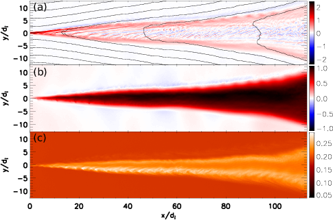
Figure 1: The exhaust of a 2D reconnection simulation (Run 1). (a) $J_{z}$ with in-plane magnetic field lines overploted, (b) $V_{ix}$, (c) $T_{i\parallel}$.

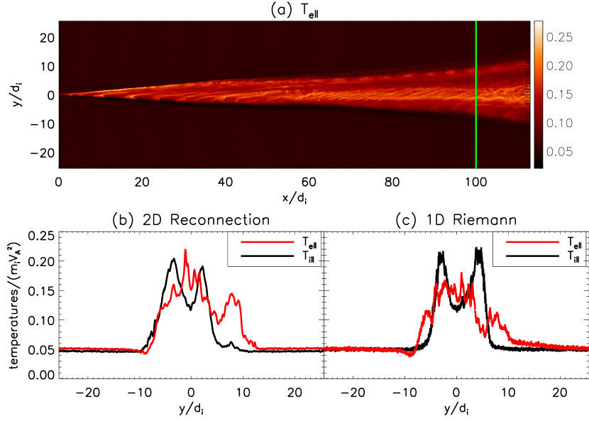
Figure 2: Comparing a 2D reconnection simulation and a 1D Riemann simulation. (a) $T_{e\parallel}$ of the 2D reconnection simulation (Run 1) exhaust, (b) profiles of $T_{e\parallel}$ and $T_{i\parallel}$ taken at the green line of (a), (c) the same profiles from the corresponding 1D Riemann simulation (Run 2).

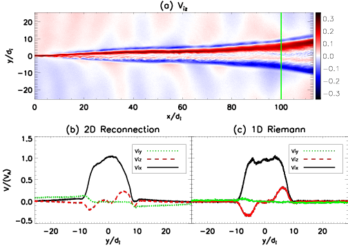
Figure 3: Similar to Fig.2, (a) $V_{iz}$ of the 2D reconnection simulation (Run 1) exhaust, (b) profiles of $V_{ix}$, $V_{iy}$ and $V_{iz}$ taken at the green line of (a), (c) the same profiles from the corresponding 1D Riemann simulation (Run 2).

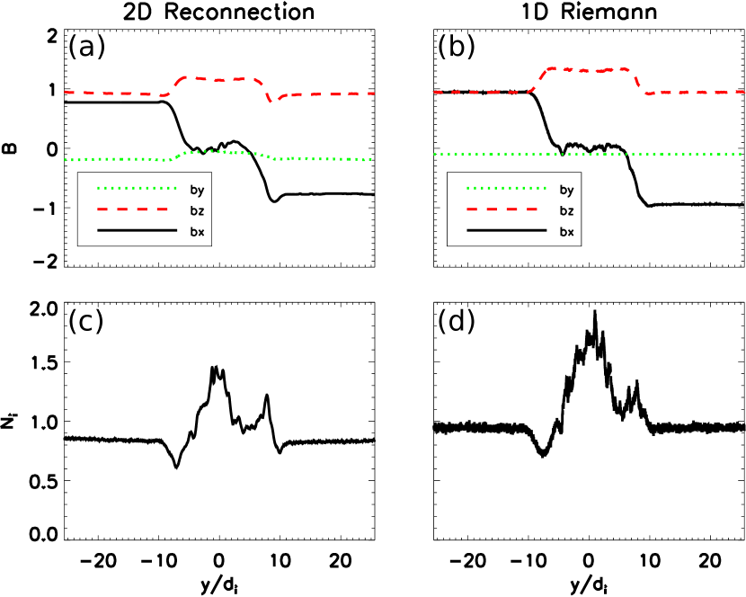
Figure 4: On the left, the profiles of $B_{x}$, $B_{y}$, $B_{z}$ (a) and $N_{i}$ (c) from the 2D reconnection simulation (Run 1). On the right, the profiles of $B_{x}$, $B_{y}$, $B_{z}$ (b) and $N_{i}$ (d) from the 1D Riemann simulation (Run 2).

Here we show that with the same parameters, Riemann simulations produce comparable results to conventional reconnection simulations. Some results of a conventional 2D reconnection simulation (Run 1) with a guide field the same as the reconnecting field are shown in Fig. 1. All data from Run 1 have been smoothed to reduce the noise. In Fig. 1(a), the in-plane magnetic field lines are overplotted on $J_{z}$. Well downstream of the x-line, the field lines turn sharply from the $x$ to the $y$ direction, indicating that the reconnecting field $B_{x}$ sharply drops to nearly zero. Note, however, that there is a strong guide field $B_{z}$ so that within the exhaust the magnetic field points dominantly in the $z$ direction. This feature is characteristic for guide field reconnection but is absent in antiparallel reconnection where Petschek’s switch-off shocks are suppressed because of pressure anisotropy Liu, Drake, and Swisdak (2012). $J_{z}$ peaks at the exhaust boundaries to support this field change. Between regions of high current is the exhaust where plasma reaches the Alfvén speed $C_{AX}$, as shown in Fig. 1(b). Ions in the exhaust are heated as shown by the ion parallel temperature increase shown in Fig. 1(c). In Fig. 2, we compare this 2D reconnection simulation (Run 1) to a 1D Riemann simulation (Run 2) with otherwise the same parameters. The second short dimension $x$ in Run 2 is a dummy dimension that is included in the simulations but can be averaged to reduce noise. Fig. 2(a) shows $T_{e\parallel}$ of the outflow from the reconnection simulation. The green cut shows the location of the profiles of parallel electron and ion temperatures shown in Fig. 2(b). Fig. 2(c) shows the corresponding profiles from the Riemann simulation at the time when the exhaust width is close to that in Fig. 2(b). In this paper profiles along $y$ from Riemann simulations with a short dimension in $x$ have all been averaged over $x$ to reduce noise. Similarly, we compare velocity, magnetic field and density profiles in Fig. 3 and Fig. 4. The comparable results from both types of simulations suggest that Riemann simulations are good proxies for the structure of outflows from conventional reconnection simulations. In the next section the structure of reconnection outflows will be discussed in more detail using Riemann simulations.

III Results and discussion

III.1 Overview

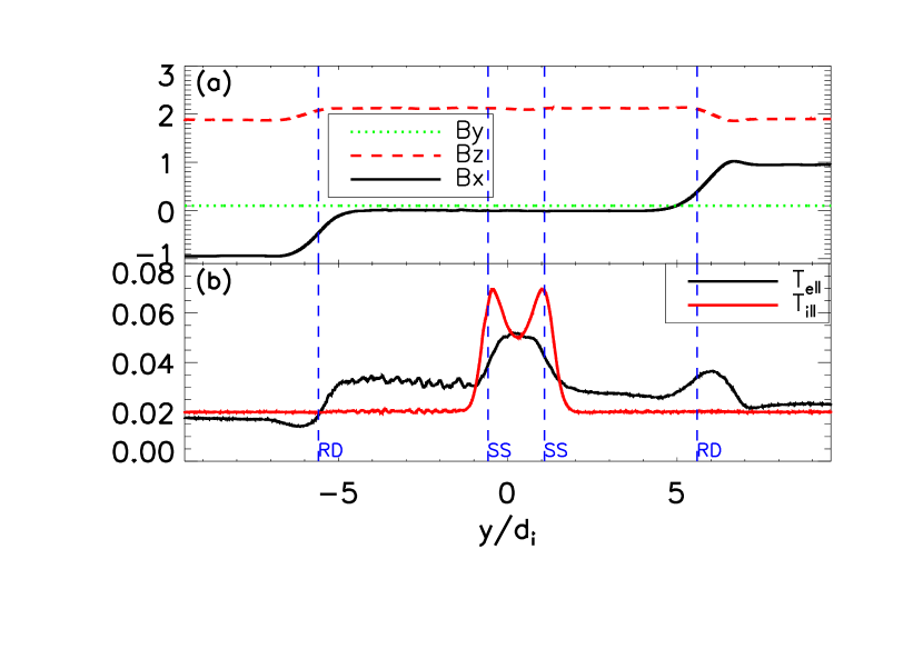
Figure 5: Profiles of $B_{x}$, $B_{y}$, $B_{z}$ (a) and $T_{e\parallel}$ and $T_{i\parallel}$ (b) from the 2D Riemann simulation (Run 3).

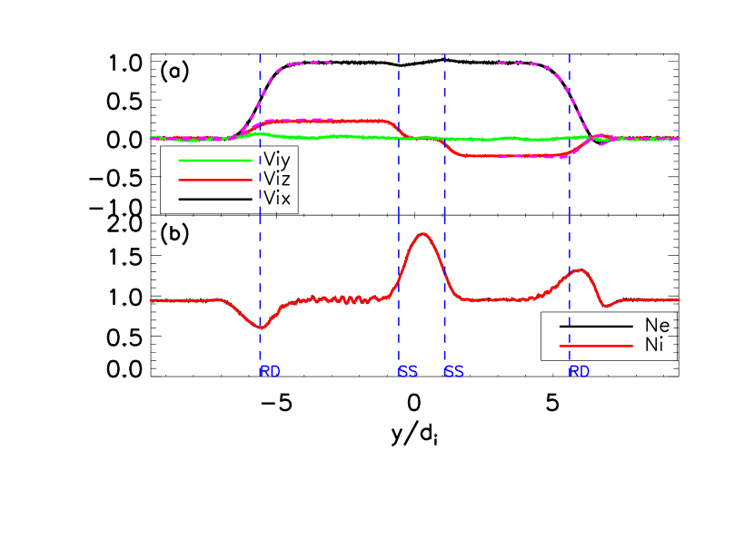
Figure 6: Profiles of $V_{ix}$, $V_{iy}$ and $V_{iz}$ (a) and $N_{e}$, $N_{i}$ (b) from the 2D Riemann simulation (Run 3). The vertical dashed lines indicate the locations of the RDs and SSs. The purple dashed lines in (a) is the MHD model predictions in Equation (2) of $V_{ix}$ and $V_{iz}$ for comparison.

In this section, we analyze a 2D Riemann simulation (Run 3), which has a guide field twice the reconnecting field, in detail to show an example of typical results. This simulation has a second dimension along $z$, the dominant magnetic field direction within the exhaust, that is long enough to capture field-aligned streaming instabilities, which will be discussed in greater detail later. After the simulation begins, the ion and electron temperatures in the exhaust increase quickly and reach nearly constant values. Then as the exhaust expands over time, the profiles of temperature and other quantities expand steadily with their shape and magnitude nearly unchanged, resulting in more and more heated particles. Snapshots of the profiles of the magnetic field, the parallel electron and ion temperatures, the bulk flows and electron and ion densities are shown in Figs. 5 and 6.

The expanding exhaust consists of nonlinear structures propagating at constant speeds away from the initial central current sheet. They are two rotational discontinuities (RDs), where magnetic fields rotate, and two slow shocks (SSs), where the fluid velocity decelerates from above to beneath the slow sonic speed ($\sim 0.2$ upstream of the shock). The structures are moving away from the midplane at nearly constant speeds. With a sufficiently large guide field and sufficiently low $\beta$ (in the case of the guide field equal to the reconnecting field, for example, $\beta\sim 0.01$), the RDs and SSs are clearly separated. An ideal MHD Riemann simulation also develops these structuresLin and Lee (1993), but the detailed properties will differ from those seen here because of the assumptions in MHD as discussed previously.

In Figs. 5 and 6 we present profiles of various quantities during the exhaust expansion. In Fig. 5(a) there is magnetic rotation at each RD (with magnetic field strength nearly unchanged) with the magnetic fields being nearly uniform throughout the region between the RDs. In Fig. 5(b), the strongest ion and electron parallel temperature increase is between the two SSs but there is also electron parallel heating between the RD and the SS, forming two shoulders in the electron parallel temperature profile. The perpendicular temperature change is negligible due to magnetic moment conservation and is therefore not shown. In Fig. 6(a) $V_{ix}$ increases across the RDs and remains nearly constant across the entire exhaust, consistent with the MHD model. $V_{iz}$ increases across each RD with opposite signs on either side of the exhaust. The resulting counterstreaming flows decreases to nearly zero across the SSs, again consistent with the MHD model. In Fig. 6(b), quasi-neutrality is well satisfied. The density has a cavity on one RD and a bump on the other one. The density does not change much across the RDs, while there is a peak between two SSs.

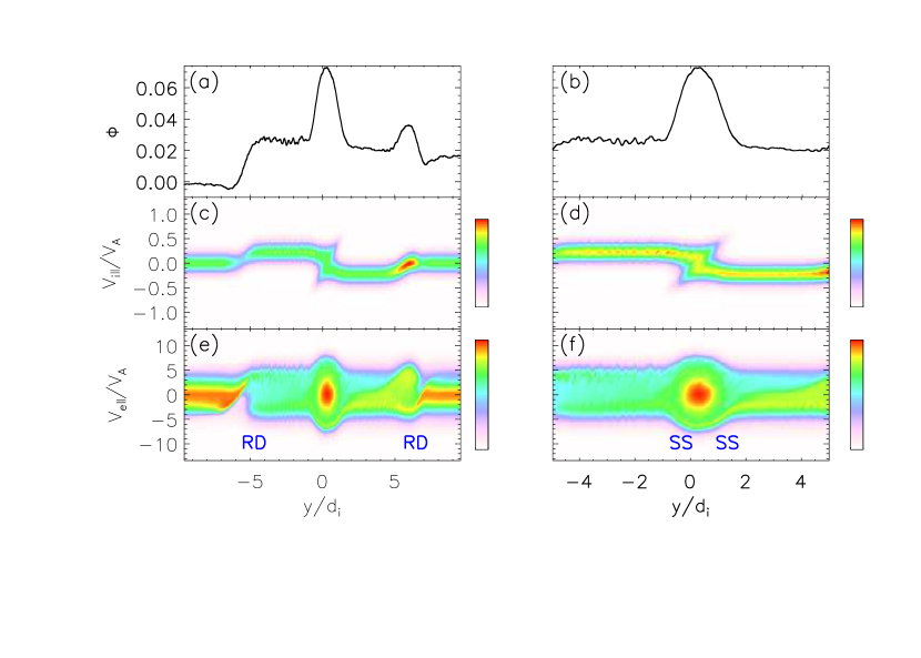
Figure 7: On the left, from top to bottom, the profile of parallel electric potential $\phi$ (a), ion phase space $y-V_{i\parallel}$ (c) and electron phase space $y-V_{e\parallel}$ (e) across the whole exhaust. On the right, the same quantities (b) (d) (f) zooming in on the region between the SSs.

We integrate the parallel electric field (smoothed over one plasma period to reduce fluctuations) to obtain the parallel electric potential as shown in Fig. 7(a) and a zoom-in of the region between the SSs in (b). Note the separate localized variations of the potential at each RD and SS. The potential gradient drives the parallel current that produces the magnetic field rotation across the RDs, maintains zero current elsewhere and enforces quasi-neutrality in the region between the SSs. These roles will be discussed in more detail in following subsections. In addition, we show the parallel phase spaces $y-V_{i\parallel}$, $y-V_{e\parallel}$ ($V_{\parallel}=\textbf{V}\cdot\textbf{B}/B$) in Fig. 7(c), (e) and the zoom-in of the region between the SSs in (d), (f). Note that in these figures positive $V_{\parallel}$ corresponds to positive $V_{y}$, and vice versa.

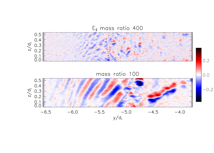
Figure 9: Parallel electric field $E_{\parallel}$ of the left RD region from two 2D Riemann simulations Run 3 (top) and Run 4 (bottom) at the same time. The two figures have the same spatial and color scales.

Before discussing in more detail the structure of the RDs and SSs we address the role of current-driven instabilities in the low $\beta$ environment considered here. Since the $z$ component of the magnetic field is the dominant component in the reconnection exhaust between the two RDs (the x component is nearly zero while $B_{y}$ remains small (see Fig. 5(a)), a long enough $z$ dimension in the simulations can capture magnetic field aligned streaming instabilities. The length of the $z$ dimension in our 2D Riemann simulations is chosen to capture electron-electron, electron-ion or ion-ion streaming instabilities. The characteristic scale lengths are $u_{b}/\omega_{pe}$ for electron-electron and electron-ion instabilites, and $V_{eth}/\omega_{pe}$ for ion-ion instabilities, where $u_{b}$ is the relative velocity between two beams and $V_{eth}$ is the electron thermal speedKrall and Trivelpiece (1973); Fujita, Ohnuma, and Adachi (1977). In Fig. 8, we show the parallel electric field $E_{\parallel}=\textbf{E}\cdot\textbf{B}/B$ in the $y-z$ plane of the Run 3 simulation listed in Table 1. There is evidence for instability at each RD (especially at the left RD), but there is no instability around or downstream of the SSs. We focus on the left RD, which exhibits a stronger instability. The turbulence is produced by the Buneman instability driven by the electron beam supporting the current at the RD. Since the width of the RD in the simulation has a $d_{i}$ scale, from Ampere’s law, the beam speed is on the order of $B_{x,u}c/4\pi ned_{i}=C_{Ax,u}$, the Alfvén speed. So the instability is expected to become weaker with higher mass ratio due to the higher electron thermal speed relative to Alfvén speed. In Fig. 9, we compare the instability in the current run (Run 3) with mass ratio 400 to that in Run 4 with mass ratio 100. We see that the instability is significantly weaker in the higher mass ratio simulations. Further, from the electron phase space in Fig. 7, we see that the instability does not significantly limit the electron beam at the left RD. Thus, the instabilities do not play a significant role either in the region around the SSs or the RDs. The driver for the instabilities and their impact on the exhaust profile will be discussed in greater detail in a follow-up paper.

III.2 Rotational discontinuity (RD)

Across an RD ions undergo a jump in velocity that can be calculated from the MHD model Lin and Lee (1993). In the limit of low upstream $\beta$,

$$\begin{split}V_{x,d}=s\frac{B_{x,d}-B_{x,u}}{\sqrt{4\pi n_{0}m_{i}}}\\ V_{z,d}=s\frac{B_{z,d}-B_{z,u}}{\sqrt{4\pi n_{0}m_{i}}}\end{split}$$ (2)

where the subscripts $u$, $d$ designate upstream and downstream of the RD and $s=sgn(V_{yu}B_{yu})$, all evaluated in the frame of the RD. Equation (2) agrees well with simulations carried out with sufficiently low upstream $\beta$. It can not only predict the total jump across the RD but also the continuous transition across the RD, if the downstream magnetic field is treated as a continuous function. As shown in Fig. 6(a), the purple dashed lines are consistent with the velocity profiles. The ion velocities in x and z directions are driven by magnetic tension in $x$ and $z$. Equation (2) indicates that $V_{z}$ downstream of the RDs has opposite signs on either side of the midplane as seen in Fig. 6(a). This leads to two ion beams traveling towards the center along the magnetic field with $V_{0}\approx|V_{z,d}|$, since $B_{z}$ is the dominant magnetic field component between the two RDs. These two beams counterstream and give rise to the two SSs. Note that in Fig. 6(a), $V_{x}$ is symmetric because $B_{x}$ and $s$ are anti-symmetric. $V_{z}$ is anti-symmetric because $B_{z}$ is symmetric while $s$ is anti-symmetric.

While the ion motion across the RDs is controlled by magnetic tension, the electrons are controlled by the localized parallel potentials at the RDs. As a result of these potentials, the electron distributions carry a localized parallel current at the RDs to support the magnetic field rotation while maintaining zero current elsewhere. This leads to partial electron confinement within the exhaust. We demonstrate this in Fig. 10. We show the phase space $y-V_{e\parallel}$ of the RD regions on the left and right of the exhaust and overplot the contours of parallel mechanical energy evaluated in the frame of the RD at the outer edge of exhaust. The mechanical energy is obtained by calculating $\frac{1}{2}m_{e}(V_{e\parallel}-V_{ramp\parallel})^{2}-e\phi$, where $\phi$ is calculated as in Fig. 7(a) and $V_{ramp\parallel}$ is the effective speed of the potential ramp along the magnetic field seen by the electrons. So $V_{ramp\parallel}=V_{ramp,y}B/B_{y}$ where $V_{ramp,y}$ is the ramp speed relative to the ${\bf E}\times{\bf B}$ drift in y direction at the ramp. We measure $V_{ramp\parallel}$ to be -2.0 for the left RD and 2.2 for the right RD. In Fig. 10 we see that the electrons mostly follow the stream lines, suggesting the potential is controlling the electron motion. In this phase space electrons with positive (negative) $V_{e\parallel}$ at the left (right) RD are streaming toward the midplane of the exhaust. As electrons enter the left RD from upstream (positive $V_{e\parallel}$) a small potential dip reflects some of the low-velocity electrons. The dominant potential (see Fig. 7(a)) then accelerates the incoming electrons across the RD, driving a localized current at the RD that supports the magnetic field jump. Most of the electrons moving toward the left RD from within the exhaust are reflected by the potential at the RD and therefore are effectively confined within the exhaust. At the right RD, the downstream outgoing electrons are first accelerated towards upstream and then decelerated to produce the localized current that supports the magnetic field jump at the RD (see the potential in Fig. 7(a)). Some of these electrons leak out of the exhaust, while some are reflected back towards the midplane. Similarly, some of the incoming electrons are accelerated into the exhaust and then decelerated. Other incoming electrons (negative $V_{e\parallel}$) are reflected back upstream by a small potential dip. Comparing both RDs, more of the downstream electrons leak across the right RD to the upstream than across the left RD. Thus, a higher fraction of electrons are confined by the RD where the electric field driving the current at the RD acts as a confining electric field. The electron confinement at either side helps to maintain zero current upstream. In the regions between the RD and the SS on either side, as in Fig. 7(e), there are electrons from the RD and electrons that have escaped from the region between the two SSs. The multiple electron populations between the RD and the SS contribute to a somewhat higher electron temperature than upstream, which is seen at the shoulders in Fig. 5(b). There is no counterpart to these shoulders in the MHD model.

Electron confinement at the edge of the exhaust was also observed in simulations reported by Egedal et al.Egedal et al. (2015); Egedal, Daughton, and Le (2012). Their reconnection simulations were in the low-$\beta$, anti-parallel regime. They found almost complete electron confinement on both sides of the exhaust in the region just downstream of the x-line. This was a consequence of a large potential which was driven by the magnetic expansion and ion demagnetization near the x-line. This mechanism, however, is not active far downstream of the x-line where ions are magnetized. Further, in guide field reconnection magnetic expansion is suppressed. As a consequence, we do not see such a large confinement potential develop, especially at the right RD.

III.3 Slow Shock (SS)

In the region between the SSs, the dynamics of both ions and electrons are controlled by the parallel potential. As shown in Fig. 6(b), upstream of the shock both ions and electrons have the same density, which is close to the ambient density $n_{0}$ upstream of the RDs. In Fig. 7(d), ions moving from upstream to downstream across the SSs are decelerated with a small fraction reflected. Some faster ions reach the SS on the other side of the exhaust and are accelerated into the region upstream of the SS. The counterstreaming ion beams around and between the SSs increase the effective ion temperature although the distributions retain beam-like features.

In contrast with the ions, the electrons are accelerated downstream across the SSs (Fig. 7(f)). Since the SSs are moving outward, some lower energy electrons are trapped by the retreating potentials and lose energy over time due to conservation of the second adiabatic invariant as the region between the SSs expands. Other higher energy electrons have high enough energy to go through the potential to escape from the region between the two SSs. The trapped electrons result in the higher electron temperature downstream of the SSs. Since it is the ion beams that are the energy source of the SSs, the electron heating represents the conversion of ion bulk flow energy to the electrons. Note that in the electron phase space shown in Fig. 7(f), there is a localized peak near (y=0, $V_{e\parallel}$=0) on the top of the rest of distributions with the maximum phase space density close to the initial distribution maximum. This is a trapped population left over from the initial formation of the RD and SS. These trapped electrons lose energy as the exhaust expands and become energetically unimportant at late time.

The two SSs are formed by the counterstreaming ion beams produced at the RDs (see Fig. 6(a)). In the frame of the exhaust downstream of the RDs the beams propagate along the nearly constant magnetic field (see Fig. 5(a)) so the resulting SSs are electrostatic shocks. The charge imbalance driven by the beams produces the jump in the parallel potential across the SSs. If there were no potential, the counterstreaming ion beams would produce an ion density of $2n_{0}$ in the central region. In contrast, due to high electron thermal velocity, only half of the electrons from either side would reach the region with counterstreaming ions. The remaining half of the electrons would never reach the region of counterstreaming ions. Thus, in the absence of the potential, the central electron density would be only $n_{0}$. The charge imbalance between ions and electrons drives the potential, which modifies the distribution functions of both species and restores quasineutrality. In the low initial $\beta$ limit of the anisotropic MHD model as is discussed in the Appendix, the speed of the SS along the magnetic field is close to $V_{0}$, just like a gas dynamic shock. This speed matches the results of simulations with sufficiently low $\beta$. If the inflowing distributions of ions and electrons into the region between the SSs were known, one could use Liouville’s theorem to kinetically express the ion and electron distributions at the center downstream of the two SSs as a function of the potential jump across the shock, which would yield their densities. Using quasineutrality one could then equate the densities of ions and electrons to solve for $\phi$ and use it to determine the central distribution functions, densities and temperatures. Thus, it is quasineutrality that controls the magnitude of the potential and the dynamics of ions and electrons. However, the major difficulty with this method is that the inflowing electron distributions into the SS from the RD are nontrivial (as discussed in the previous subsection). We will further discuss the quasineutrality requirement in the low-$\beta$ regime in the next section.

IV Scaling of heating and energy partition in the low-$\beta$ regime

IV.1 Justification of 1D Riemann simulations

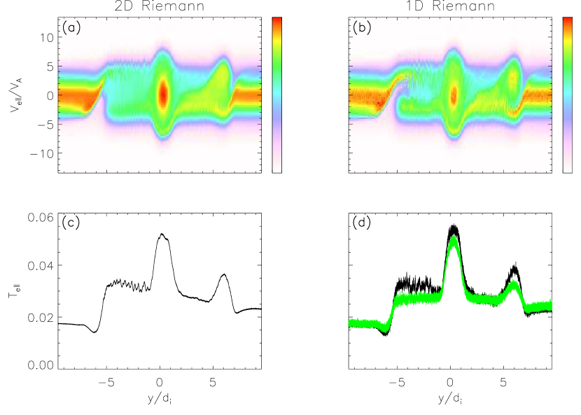
Figure 11: Comparing a 2D Riemann simulation and a 1D Riemann simulation. On the left from the 2D Riemann simulation (Run 3), the electron phase space $y-V_{e\parallel}$ (a) and the profile of $T_{e\parallel}$ (c). On the right the corresponding quantities (b) (d) from the 1D Riemann simulation (Run 5). The green line in (d) is the $T_{e\parallel}$ profile from Run 13 with mass ratio 1600.

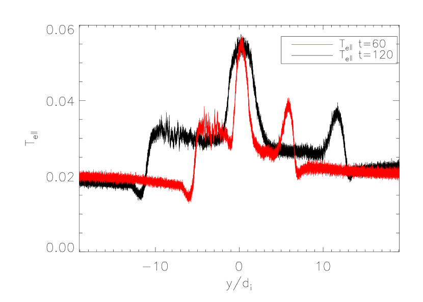
Figure 12: The parallel electron temperature profiles of Run 14 at t=60 and t=120.

To explore the scaling of ion and electron heating in the low-$\beta$ regime we perform a series of 1D Riemann simulations. By ignoring the $z$ direction, we eliminate the possible development of streaming instabilities such as those seen in Fig. 8. However, these instabilities have little effect on the system’s development. To demonstrate this we show in Fig. 11 a comparison between a 2D Riemann simulation in the y-z plane (Run 3) and a 1D Riemann (Run 5) simulation based on the same parameters. Panels a and b show the phase spaces and panels c and d (black line) show the $T_{e\parallel}$ profiles. The similarity of the panels suggests that the eliminated instabilities that did develop in the 2D simulation are too weak to have a significant impact on the results. Also we show in panel d (green line) the $T_{e\parallel}$ profile from Run 13 with a mass ratio 1600 and otherwise the same physical parameters as Run 5 to demonstrate that the results are not sensitive to the mass ratio as long as it is high enough. In addition, we perform a 1D Riemann simulation (Run 14) doubling the domain size in y of Run 5, so that we can double the simulation time from 60 to 120. We show the electron parallel temperature profiles at t=60 and t=120 in Fig. 12. We demonstrate that the structures and heating remains the same as the exhaust further expands over time. Hence, in the next section we will use 1D Riemann simulations to scan the low-$\beta$ regime.

IV.2 Scaling of electron and ion heating with the released magnetic energy

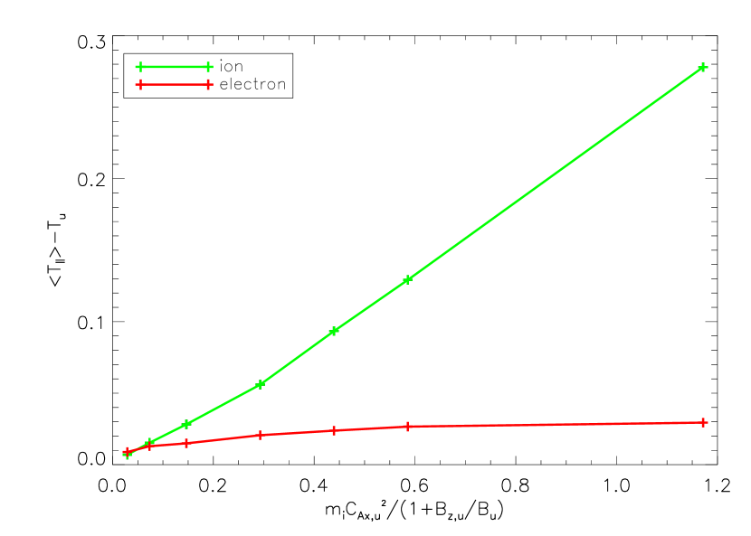
Figure 13: The scaling of parallel heating of ions and electrons as a function of available magnetic energy per particle using data from Runs 5-10

Here we present a series of simulations (Runs 5-11) in which the only difference in the initial profiles of the physical quantities are the magnitudes of the upstream magnetic fields. For these runs the electron $\beta$ varies between 0.1 and 0.0025. For the lower $\beta$, the higher mass ratio is needed to ensure that the electron thermal speed exceeds the characteristic ion flow, RD and SS effective speeds along the field, etc. The requirements on the mass ratio will be discussed more in the next subsection. In Fig. 13, we plot the variation of the ion and electron temperature increase averaged over the region between the two SSs. The horizontal axis is the available magnetic energy per particle in the low-$\beta$ limit $m_{i}C_{Ax,u}^{2}/(1+B_{z,u}/B_{u})$ derived from anisotropic MHD (see the Appendix).

We see in Fig. 13 that the ion heating is proportional to the available magnetic energy per particle in the low $\beta$ limit as expected, while the electron heating reaches a plateau in the low-$\beta$ limit. In contrast, previous observational and computational reconnection scaling studies suggest that the electron heating should exhibit a linear scalingPhan et al. (2013); Shay et al. (2014). However, these previous studies only focused on the $\beta$ of order unity regime and therefore did not reach low enough $\beta$ to see the saturation of the electron heating. We find one simulation (number 302) in Shay’s paperShay et al. (2014) with both initial ion to electron temperature ratio and guide field to reconnecting field ratio equal to one that can be compared with one of our simulations. We confirm that our highest $\beta$ run (Run 6) produces comparable electron heating to Shay’s simulation if we renormalize our run’s available magnetic energy per particle to be the same as Shay’s run and we calculate the heating averaged over the whole exhaust as Shay did. Therefore, the Riemann simulation results here are consistent with the previous results at higher $\beta$. The physical reason for the saturation of electron heating with available magnetic energy is discussed in the next subsection. The consequence is that the ion heating dominates over electron heating in the limit of low upstream $\beta$.

The SS potential can be evaluated by integrating the electron parallel momentum equation across the SS neglecting the inertia termHaggerty et al. (2015),

$$e\Delta\phi=\Delta T_{e\parallel}+\int dsT_{e\parallel}\nabla_{\parallel}\ln(n)+\\ \int ds(T_{e\parallel}-T_{e\bot})\nabla_{\parallel}\ln(B),$$ (3)

with $ds$ the distance along the local magnetic field. The third term on the right can be neglected because the magnetic field is nearly constant across the SS. The potential therefore scales like the electron temperature. Since this is small in the low $\beta$ limit, the potential is insufficient to significantly alter the velocity of the ions as they cross the SS. The consequence is that ion reflection by the shock potential does not take place, which eliminates the reflected ion beams upstream of the slow shock that play such an important role in high Mach number parallel shocks. Downstream of the SS the ions remain as distinct counterstreaming beams with essentially no mixing. Although the counterstreaming ion beams have significant free energy, the ion-ion two stream instability along the field lines is stable since the electron temperature is low with the consequence that the ion beam speed is higher than the sound speed $\sqrt{T_{e\parallel}/m_{i}}$Fujita, Ohnuma, and Adachi (1977). As a crosscheck we carried out a 2D test simulation with uniform magnetic fields and parallel counterstreaming ion beams with speed higher than sound speed. We did not observe any instabilities develop to release the energy associated with the counterstreaming ion beams. This result is consistent with Fujita et al.Fujita, Ohnuma, and Adachi (1977).

IV.3 The saturation of electron heating at low $\beta$

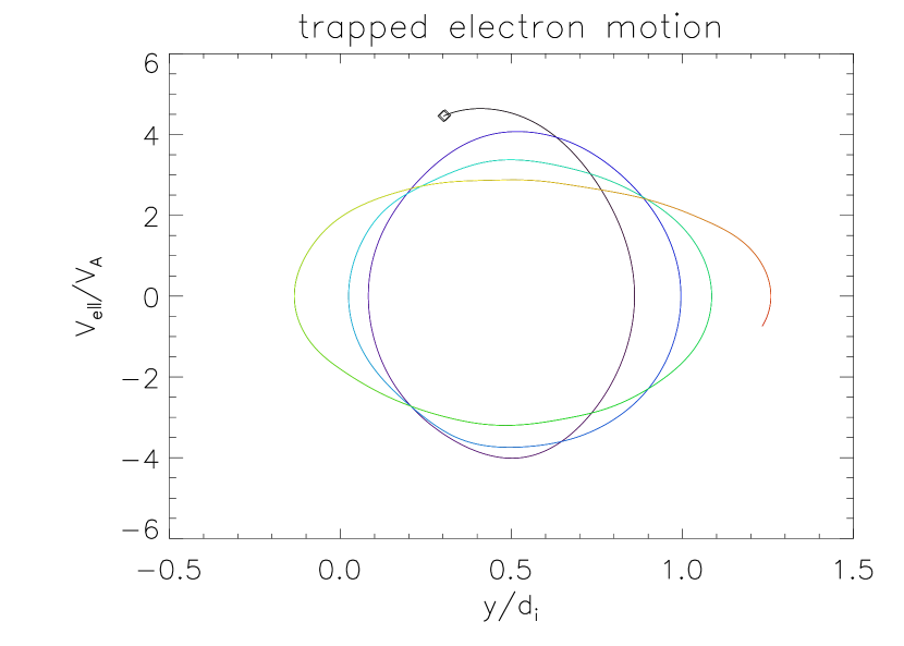
Figure 14: A test particle trajectory in $y-V_{e\parallel}$ phase space using the smoothed magnetic fields and parallel electric potential from Run 11. The trajectory begins at the diamond and changes color from black to red during the particle motion.

Here we discuss the physics behind the saturation of electron heating in the low $\beta$ regime. The electron parallel temperature increase across the RD in our simulations is small because the electron thermal speeds are much higher than the streaming velocities at the RDs required to form the current needed to switch-off $B_{x}$. As the electrons downstream of the RD cross the SS, the electrons gain energy because of the high potential between the SSs. Electrons below a critical speed $V_{trap}$ in the lab frame will get trapped between the SSs, while those above it will free stream across both SSs to the other side of the exhaust. We evaluate $V_{trap}$ in the following. We first point out that an electron with this critical velocity upstream of the first SS will, after passing through both SSs, reach zero velocity in the frame of the second. We trace an electron with zero velocity just outside of the second SS backwards in time. Before crossing the second SS this electron has a velocity $V_{\phi}=\sqrt{2\phi/m_{e}}$ in the frame of the SS. Switching to the frame of the first potential, its parallel velocity is $V_{\phi}+2V_{s}$ where $V_{s}$ is the effective speed of the SS along the magnetic field in the lab frame. In this frame before crossing the first potential, the speed is $\sqrt{(V_{\phi}+2V_{s})^{2}-V_{\phi}^{2}}=2\sqrt{V_{s}V_{\phi}+V_{s}^{2}}$. Now changing back to the lab frame, we obtain the critical velocity $V_{trap}=2\sqrt{V_{s}V_{\phi}+V_{s}^{2}}-V_{s}$. The trapped electrons then undergo adiabatic deceleration in the expanding trap. We demonstrate this in Fig. 14 using a test particle trajectory in the phase space $y-V_{e\parallel}$. Here we have applied the time dependent background profiles of magnetic fields and smoothed parallel electric potentials from Run 11. The potential profile is obtained from equation (3), which is close to that from directly integrating parallel electric fields as in Fig. 7(a). The particle starts at the diamond point and moves from black to red color over time, decelerating towards zero velocity.

From charge neutrality the flux of ions and electrons that remains between the SSs must be equal. In the low $\beta$ limit, the upstream ion is an incoming beam with speed $2V_{s}$, so the incoming ion flux is $2n_{0}V_{s}$. All of these ions remain between the two SSs. The trapped electrons make up the dominant component of the downstream electrons since the untrapped electrons transit out of the region between the SSs very quickly. Thus, the incoming flux of electrons that will be trapped must match the total incoming flux of ions. We take the upstream thermal speed $V_{eth,u}\gg V_{s}$ (so $\beta$ can not be too low) and $V_{\phi}\gg V_{s}$ so $V_{trap}$ simplifies to $2\sqrt{V_{s}V_{\phi}}$. The upstream electrons with velocities between v=0 and $2\sqrt{V_{s}V_{\phi}}$ will be trapped. Taking $V_{eth,u}\gg V_{trap}$, the fraction of trapped electrons is $V_{trap}/V_{et,u}$. The electron flux is then given by $n_{0}V_{trap}^{2}/2V_{eth,u}$. Equating the incoming fluxes of the two species, we have

$$n_{0}\frac{V_{trap}^{2}}{2V_{eth,u}}\sim 2n_{0}V_{s}$$ (4)

to obtain $V_{\phi}\sim V_{eth,u}$ or $e\phi\sim T_{e,u}$. Therefore, $T_{e,d}\sim e\phi\sim T_{e,u}$. Thus, the electron heating can not be very strong even with large available magnetic energy per particle and the electron heating reaches a plateau as shown in Fig. 13. Physically, this is because the electron heating is limited by the amplitude of the potential across the SSs. A very large potential does not develop because it would trap too many electrons compared with the modest increase in ion density (a factor of two) and so charge neutrality would be violated.

The conditions used above, $V_{eth,u}\sim V_{\phi}\gg V_{s}$, are satisfied in our simulations as long as the ion-to-electron mass ratio is sufficiently large.

IV.4 Partitioning of the ion energy gain

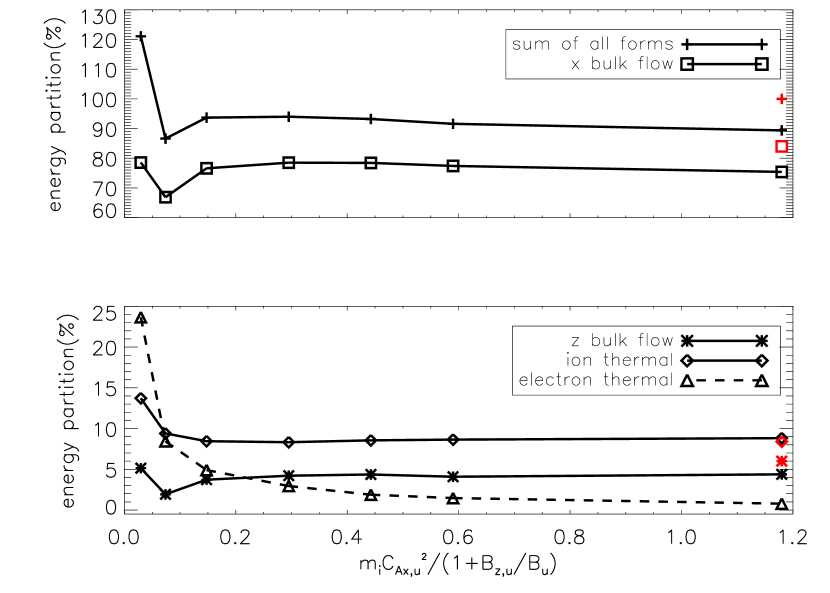
Figure 15: Energy partition into different forms of kinetic energy as a function of available magnetic energy per particle. The corresponding predicted partition by anisotropic MHD in the low initial $\beta$ limit is plotted in red

Magnetic energy flows into the exhaust and is converted into different forms of energy. As expected from the dominance of the ion temperature in Fig. 13, in the low-$\beta$ limit the ion thermal energy dominates the electron thermal energy. In this limit, the electron thermal energy upstream and downstream can be neglected. The ion energy gain across the exhaust can be calculated using the anisotropic MHD solution in the Appendix. The available magnetic energy per particle was calculated previously to be $m_{i}C_{Ax,u}^{2}/(1+B_{z,u}/B_{u})$. The released magnetic energy partitions into three distinct fractions: $(B_{u}+B_{z,u})/(2B_{u})$ for ion bulk flow energy associated with $V_{ix}$; $(B_{u}-B_{z,u})(2B_{z,u}-B_{u})/(2B_{u}^{2})$ for ion bulk flow energy in $V_{iz}$; and $(B_{u}-B_{z,u})^{2}/B_{u}^{2}$ for ion thermal energy. The fractions total to unity. They can be tested by the same set of simulations used in Fig. 13. In the exhaust, we calculate the ratio of these components of the ion energy (normalized by the number of ions) to the available magnetic energy per particle $m_{i}C_{Ax,u}^{2}/(1+B_{z,u}/B_{u})$ and we plot them as a function of $m_{i}C_{Ax,u}^{2}/(1+B_{z,u}/B_{u})$ in Fig. 15. The summation of the fraction of all forms is close to unity at low-$\beta$, suggesting that our prediction of the available magnetic energy per particle is correct. Each line approaches a constant and agrees reasonably well with the corresponding predicted partition by anisotropic MHD in the low initial $\beta$ limit plotted in red.

V Conclusion

In this paper we report the results of low-$\beta$ guide field particle-in-cell Riemann simulations with high ion-electron mass ratio to explore the particle heating in reconnection outflows far downstream from the x-line. Comparison with conventional reconnection simulations shows that Riemann simulations can produce comparable results when the simulation parameters overlap. Thus, Riemann simulations are good proxies of reconnection simulations and can be useful to explore the low-$\beta$ regime with more realistic parameters than is possible with full 2D reconnection simulations.

The results of Riemann simulations in the low-$\beta$ regime show that the RDs and SSs associated with reconnection clearly separate from one another, steadily moving outwards from the exhaust midplane. The steady expansion of the exhaust, as long as the domain is large enough, should continue without bound, suggesting that particle heating in the exhausts can extend to macroscopic scales in the corona. There is ion and electron heating between two SSs and electron heating between the RD and SS. The latter produces shoulders in the electron temperature profile that extend across the entire exhaust. The heating mechanisms downstream of the SSs differ from those between the RD and SS. Ions are accelerated by the RD magnetic field tension and gain bulk flow energy along the $x$ direction (the reconnection exhaust) and in the out-of-plane $z$ direction. Electrons are controlled by the electric potential that forms to produce the localized parallel current to support the magnetic rotation at the RDs and to maintain zero current elsewhere. These potentials partially confine electrons within the exhaust. The two RDs, however, have different confinement characteristics. A higher fraction of electrons are confined by the RD where the electric field driving the current at the RD acts in the same direction as a confining electric field. The ion beams produced at the RDs counterstream across the midplane of the exhaust and create a region of high density (a factor of two above the upstream density) that defines the domain between the SSs. The increase of the ion density leads to a region of high potential between the SSs to confine downstream electrons to maintain charge neutrality. The potential accelerates electrons from upstream of the SSs towards downstream and traps a fraction of them, modestly increasing the downstream electron temperature.

The heating of ions and electrons as a function of available magnetic energy per particle reveals distinct differences between the two species. The ion heating exhibits a roughly linear scaling with available magnetic energy while the electron heating reaches a plateau in the low-$\beta$ limit. The consequence is that the electron energy increment is only of the same order as the upstream temperature. This is in contrast to the linear scaling for both ions and electrons that would be expected if the heating were simply proportional to the available magnetic energy per particlePhan et al. (2013, 2014). The special scaling for electrons originates from the quasineutrality requirement, which prohibits strong electron heating even with large available magnetic energy per particle. As a result of this scaling, ion heating dominates over electron heating in the low-$\beta$ limit and the energy partition reduces to an anisotropic MHD prediction with electron energy gain neglected.

Rowan et al.Rowan, Sironi, and Narayan (2019) have also investigated guide field reconnection heating and energy partition with realistic mass ratio and low $\beta$. They concluded that electrons rather than ions gained most of the released energy in the strong guide field limit. However, they explored the trans-relativistic regime with magnetization $\sigma=B^{2}/4\pi nm_{i}c^{2}\sim 0.1$. This translates to an electron Alfvén speed close to $c$. Around the x-line and along magnetic separatrices the electron velocity approaches the electron Alfvén speed so electrons can approach relativistic velocities in a single x-line encounter. In the non-relativistic regime under consideration here, in which most electrons bypass the x-line and enter the exhaust downstream, the electrons gain negligible energy in a single passage through the exhaust. As a consequence, it is the ions rather than electrons that gain significant energy in a single interaction with the rotational discontinuity that bounds the reconnection exhaust. The ions therefore gain the most energy in the non-relativistic limit.

The fundamental physics revealed in this study has broad implications to the inner heliosphere and the corona where reconnection plays a role in magnetic energy conversion. This study specifically raises questions about how electrons gain significant energy in the single x-line model of reconnection-driven flare energy release. With the electron energy gain controlled by potentials in our picture, neither very energetic electron nor very strong electron heating can take place in single x-line reconnection exhausts. The conventional picture of strong electron heating at the slow shocks produced during reconnection Tsuneta (1996); Longcope and Bradshaw (2010) therefore fails. Further, the generation of an energetic electron powerlaw tail up to energies of the order of an MeV as observed in large solar flaresLin et al. (2003), is also not possible in a single exhaust. This study suggests that other mechanisms are required to explain electron energy gain in solar flares, such as multiple x-line reconnection Drake et al. (2006); Drake, Swisdak, and Fermo (2013); Dahlin, Drake, and Swisdak (2015, 2017).

*

Appendix A Calculation of anisotropic MHD solution

Since we are looking at symmetric reconnection, we only need to consider one side of the domain with one RD and one SS. According to Lin et al.Lin and Lee (1993), with pressure anisotropy, the Rankine-Hugoniot jump conditions of each discontinuity (RD or SS) are:

$$\begin{split}&[\rho V_{y}]=0\\ &[\rho V_{y}\textbf{V\textsubscript{t}}-\frac{B_{y}\textbf{B\textsubscript{t}}}{4\pi}+\frac{B_{y}\textbf{B\textsubscript{t}}}{8\pi}(\beta_{\parallel}-\beta_{\perp})]=0\\ &[\rho V_{y}^{2}+P_{\perp}+\frac{B^{2}}{8\pi}+\frac{B_{y}^{2}}{8\pi}(\beta_{\parallel}-\beta_{\perp})]=0\\ &[\left(\frac{1}{2}\rho V^{2}+\frac{5}{2}P+\frac{B^{2}}{4\pi}-\frac{B^{2}}{24\pi}(\beta_{\parallel}-\beta_{\perp})\right)V_{y}-\left(1-\frac{1}{2}(\beta_{\parallel}-\beta_{\perp})\right)\frac{B_{y}\textbf{B\textsubscript{t}}}{4\pi}\cdot\textbf{V\textsubscript{t}}\\ &-\left(1-\frac{1}{2}(\beta_{\parallel}-\beta_{\perp})\right)\frac{B_{y}^{2}}{4\pi}V_{y}]=0\\ &[B_{y}\textbf{V\textsubscript{t}}-V_{y}\textbf{B\textsubscript{t}}]=0\end{split}$$ (5)

,where $\rho=nm_{i}$, $\beta_{\parallel}$ and $\beta_{\perp}$ are plasma beta parallel and perpendicular to the local field, and $P=(P_{\parallel}+2P_{\perp})/3$. Subscript ”t” means tangential to the shock surface.

In the low initial $\beta$ limit, the perpendicular temperature (and thus pressure) throughout the solution can be neglected due to the conservation of magnetic moment. Also the parallel pressure upstream of the RD can be neglected. Similar to Liu et al.Liu, Drake, and Swisdak (2012), since $B_{y}\ll B$ and $V_{y}$ is of the order of $C_{Ay}$ in reconnection, to the lowest order the equations can be simplified to the following:

$$\begin{split}&[\rho V_{y}]=0\\ &[\rho V_{y}\textbf{V\textsubscript{t}}-\frac{B_{y}\textbf{B\textsubscript{t}}}{4\pi}(1-\frac{\beta_{\parallel}}{2})]=0\\ &[\frac{B_{t}^{2}}{8\pi}]=0\\ &[\left(\frac{1}{2}\rho\textbf{V\textsubscript{t}}^{2}+\frac{5}{2}3P_{\parallel}+\frac{B_{t}^{2}}{4\pi}-\frac{B_{t}^{2}}{24\pi}\beta_{\parallel}\right)V_{y}-\left(1-\frac{1}{2}\beta_{\parallel}\right)\frac{B_{y}\textbf{B\textsubscript{t}}}{4\pi}\cdot\textbf{V\textsubscript{t}}]=0\\ &[B_{y}\textbf{V\textsubscript{t}}-V_{y}\textbf{B\textsubscript{t}}]=0\end{split}$$ (6)

There are a total of 7 jump conditions and 7 downstream unknowns here applicable to each RD or SS. The unknowns are $B_{x},B_{z},V_{x},V_{y},V_{z},n,T_{\parallel}$. Note that the jump conditions for the RD, under the low-$\beta$ assumption, will reduce to that of isotropic MHD. In addition, there are three more unknowns: the speeds in y direction in the lab frame of the SS, RD and the plasma upstream of the RD. Note that $V_{x}$ and $V_{z}$ upstream of the RD are zero in the lab frame. Since the reconnection is symmetric here, we also have three more constraint equations for the quantities downstream of SS, which are $B_{x}=0,V_{y}=0,V_{z}=0$ in the lab frame. So with the same number of equations as the unknowns, we can obtain a solution for all these physical quantities.

In the solution, the speeds in y direction in the lab frame of the SS, RD and the plasma upstream of RD are $-sV_{0}B_{y,u}/B_{u}$, $-s(C_{Ay,u}-V_{0}B_{y,u}/B_{u})$ and $sV_{0}B_{y,u}/B_{u}$. Other quantities are: between the RD and SS, $B_{x}=0,B_{z}=B_{u},n=n_{0},V_{x}=-sB_{x,u}/\sqrt{4\pi n_{0}m_{i}},V_{z}=s(B_{u}-B_{z,u})/\sqrt{4\pi n_{0}m_{i}},T_{\parallel}=0,T_{\perp}=0$. Between the two SSs, $B_{x}=0,B_{z}=B_{u},n=2n_{0},V_{x}=-sB_{x,u}/\sqrt{4\pi n_{0}m_{i}},V_{z}=0,T_{\parallel}=((B_{u}-B_{z,u})/\sqrt{4\pi n_{0}m_{i}})^{2},T_{\perp}=0$.

There are a few notable features of this solution. In the lab frame there is no ${\bf E}\times{\bf B}$ flow in y-z plane between RD and SS as well as downstream of SS, so the field lines in the exhaust are simply stationary in y-z plane. The speed of the slow shock, if converted to a speed along the magnetic field, is about $V_{0}$, which is the same as the inflowing speed along the fields upstream of SS. The plasma upstream of the RD has an nonzero incoming speed and the RD is traveling with upstream $C_{Ay}$ relative to the upstream plasma.

Table 1: Simulation parameters

Run	$m_{i}/m_{e}$	$B_{x,a}$	$B_{z,a}$	$T_{i}=T_{e}$	dims	$L_{y}\times L_{x}\times L_{z}$	$c^{2}$	dx	dt
1	25	1	1	0.05	2	102.4$\times$409.6 $\times$ 0	$45$	0.0125	5.9e-3
2	25	1	1	0.05	1	102.4$\times$0.2$\times$0	$45$	0.0125	5.9e-3
3	400	1	2	0.02	2	22.9$\times$0$\times$0.54	$720$	0.0007	2e-4
4	100	1	2	0.02	2	22.9$\times$0$\times$1.08	$180$	0.0014	6e-4
5	400	1	2	0.02	1	22.9$\times$0$\times$0.011	$720$	0.0007	2e-4
6	400	$1/\sqrt{20}$	$1/\sqrt{20}$	0.005	1	45.8$\times$0$\times$0.0022	$720$	0.00056	1.56e-4
7	400	$\sqrt{0.125}$	$\sqrt{0.125}$	0.005	1	45.8$\times$0$\times$0.0022	$720$	0.00056	1.56e-4
8	400	$\sqrt{0.25}$	$\sqrt{0.25}$	0.005	1	45.8$\times$0$\times$0.0022	$720$	0.00056	1.56e-4
9	400	$\sqrt{0.5}$	$\sqrt{0.5}$	0.005	1	45.8$\times$0$\times$0.0022	$720$	0.00056	1.66e-4
10	400	$\sqrt{0.75}$	$\sqrt{0.75}$	0.005	1	45.8$\times$0$\times$0.0022	$720$	0.00056	1.56e-4
11	400	1	1	0.005	1	45.8$\times$0$\times$0.00186	$720$	0.000466	1.3e-4
12	800	$\sqrt{2}$	$\sqrt{2}$	0.005	1	45.8$\times$0$\times$0.0011	$1440$	0.00028	5.5e-5
13	1600	1	2	0.02	1	22.9$\times$0$\times$0.00447	$2880$	0.00028	4e-5
14	400	1	2	0.02	1	45.8$\times$0$\times$0.011	$720$	0.0007	2e-4

Figure 8: Parallel electric field $E_{\parallel}$ from the 2D Riemann simulation (Run 3). Note the different axis scales.

Figure 10: The phase space $y-V_{e\parallel}$ of the regions around the RDs on the left and right of the exhaust with the contours of parallel mechanical energy evaluated using the potential at this time in the frame of the RD potential ramp at the outer edge to show the approximate phase space stream lines of electrons under the potential.

References

- Guidoni and Longcope (2010) S. E. Guidoni and D. W. Longcope, The Astrophysical Journal 718, 1476 (2010).
- Guidoni and Longcope (2011) S. E. Guidoni and D. W. Longcope, The Astrophysical Journal 730, 90 (2011).
- Drake et al. (2003) J. F. Drake, M. Swisdak, C. Cattell, M. A. Shay, B. N. Rogers, and A. Zeiler, Science 299, 873 (2003).
- Pritchett and Coroniti (2004) P. L. Pritchett and F. V. Coroniti, Journal of Geophysical Research: Space Physics 109 (2004), 10.1029/2003JA009999, a01220.
- Liu, Drake, and Swisdak (2012) Y.-H. Liu, J. F. Drake, and M. Swisdak, Physics of Plasmas 19, 022110 (2012), http://dx.doi.org/10.1063/1.3685755.
- Shay et al. (2014) M. A. Shay, C. C. Haggerty, T. D. Phan, J. F. Drake, P. A. Cassak, P. Wu, M. Øieroset, M. Swisdak, and K. Malakit, Physics of Plasmas 21, 122902 (2014), http://dx.doi.org/10.1063/1.4904203.
- Haggerty et al. (2015) C. C. Haggerty, M. A. Shay, J. F. Drake, T. D. Phan, and C. T. McHugh, Geophysical Research Letters 42, 9657 (2015), 2015GL065961.
- Egedal et al. (2015) J. Egedal, W. Daughton, A. Le, and A. L. Borg, Physics of Plasmas 22, 101208 (2015), http://dx.doi.org/10.1063/1.4933055.
- Drake et al. (2009a) J. F. Drake, M. Swisdak, T. D. Phan, P. A. Cassak, M. A. Shay, S. T. Lepri, R. P. Lin, E. Quataert, and T. H. Zurbuchen, Journal of Geophysical Research: Space Physics 114 (2009a), 10.1029/2008JAO13701.
- Drake et al. (2009b) J. F. Drake, P. A. Cassak, M. A. Shay, M. Swisdak, and E. Quataert, The Astrophysical Journal 700, L16 (2009b).
- Daughton et al. (2011) W. Daughton, V. Roytershteyn, H. Karimabadi, L. Yin, B. J. Albright, B. Bergen, and K. J. Bowers, Nature Physics 7, 539 (2011).
- Dahlin, Drake, and Swisdak (2014) J. T. Dahlin, J. F. Drake, and M. Swisdak, Physics of Plasmas 21, 092304 (2014), http://dx.doi.org/10.1063/1.4894484.
- Dahlin, Drake, and Swisdak (2015) J. T. Dahlin, J. F. Drake, and M. Swisdak, Physics of Plasmas 22, 100704 (2015), http://dx.doi.org/10.1063/1.4933212.
- Phan et al. (2013) T. D. Phan, M. A. Shay, J. T. Gosling, M. Fujimoto, J. F. Drake, G. Paschmann, M. Øieroset, J. P. Eastwood, and V. Angelopoulos, Geophysical Research Letters 40, 4475 (2013).
- Phan et al. (2014) T. D. Phan, J. F. Drake, M. A. Shay, J. T. Gosling, G. Paschmann, J. P. Eastwood, M. Øieroset, M. Fujimoto, and V. Angelopoulos, Geophysical Research Letters 41, 7002 (2014), 2014GL061547.
- Lin and Lee (1993) Y. Lin and L. C. Lee, Space Science Reviews 65, 59 (1993).
- Lin and Swift (1996) Y. Lin and D. W. Swift, Journal of Geophysical Research: Space Physics 101, 19859 (1996).
- Scholer and Lottermoser (1998) M. Scholer and R.-F. Lottermoser, Geophysical Research Letters 25, 3281 (1998).
- Cremer and Scholer (1999) M. Cremer and M. Scholer, Geophysical Research Letters 26, 2709 (1999).
- Cremer and Scholer (2000) M. Cremer and M. Scholer, Journal of Geophysical Research: Space Physics 105, 27621 (2000).
- Liu, Drake, and Swisdak (2011a) Y.-H. Liu, J. F. Drake, and M. Swisdak, Physics of Plasmas 18, 062110 (2011a), http://dx.doi.org/10.1063/1.3601760.
- Liu, Drake, and Swisdak (2011b) Y.-H. Liu, J. F. Drake, and M. Swisdak, Physics of Plasmas 18, 092102 (2011b), http://dx.doi.org/10.1063/1.3627147.
- Zeiler et al. (2002) A. Zeiler, D. Biskamp, J. F. Drake, B. N. Rogers, M. A. Shay, and M. Scholer, Journal of Geophysical Research: Space Physics (1978–2012) 107, SMP 6 (2002).
- Krall and Trivelpiece (1973) N. A. Krall and A. W. Trivelpiece, Principles of plasma physics (McGraw-Hill, 1973) p. 449.
- Fujita, Ohnuma, and Adachi (1977) T. Fujita, T. Ohnuma, and S. Adachi, Plasma Phys. 19, 875 (1977).
- Egedal, Daughton, and Le (2012) J. Egedal, W. Daughton, and A. Le, Nature Physics 8 (2012), 10.1038/NPHYS2249.
- Rowan, Sironi, and Narayan (2019) M. E. Rowan, L. Sironi, and R. Narayan, The Astrophysical Journal 873, 2 (2019).
- Tsuneta (1996) S. Tsuneta, The Astrophysical Journal 456, 840 (1996).
- Longcope and Bradshaw (2010) D. W. Longcope and S. J. Bradshaw, The Astrophysical Journal 718, 1491 (2010).
- Lin et al. (2003) R. P. Lin, S. Krucker, G. J. Hurford, D. M. Smith, H. S. Hudson, G. D. Holman, R. A. Schwartz, B. R. Dennis, G. H. Share, R. J. Murphy, A. G. Emslie, C. Johns-Krull, and N. Vilmer, The Astrophysical Journal Letters 595, L69 (2003).
- Drake et al. (2006) J. F. Drake, M. Swisdak, H. Che, and M. A. Shay, Nature 443, 553 (2006).
- Drake, Swisdak, and Fermo (2013) J. F. Drake, M. Swisdak, and R. Fermo, The Astrophysical Journal Letters 763, L5 (2013).
- Dahlin, Drake, and Swisdak (2017) J. T. Dahlin, J. F. Drake, and M. Swisdak, Physics of Plasmas 24, 92110 (2017).