Chapter 0 Introduction

1 History

In this MS thesis, we will consider the electromagnetic field of an accelerating charge. Accelerated moving charges according to the laws of electrodynamics as described by James Clerk Maxwell [Maxwell61] must emit electromagnetic waves. In 1865 Maxwell derived a system of equations which can now be expressed in differential or integral form describing an electromagnetic field and its connection with electric charges and currents in vacuum and continuum. Together with the expression for the Lorentz force, which specifies the measure of the effect of an electromagnetic field on charged particles, these equations form a complete system of classical electrodynamics. The equations formulated by Maxwell on the basis of experimental results accumulated by the middle of the 1800s, played a key role in the development of theoretical physics and had a strong influence not only on all areas of physics directly related to electromagnetism, but also on many later fundamental theories, like special theory of relativity.

In 1897 Joseph Larmor [Larmor1897] first calculated the total power radiated by a non-relativistic point charge as it decelerated or accelerated. The Larmor radiation formula describes a uniformly accelerating single point charge which emits radiation toward infinity.

In 1955, Gold and Bondi wrote a paper [BondiGold] where they established the production of the electromagnetic field by a uniformly accelerated charged particle. This was a problem that had been considered before but without finding the complete solution. Later, a new question was raised : could the equivalence principle apply to such a situation?

The equivalence principle is that used by Albert Einstein in the derivation of the general theory of relativity. Its formulation briefly can be expressed as: ‘the gravitational and inertial masses of a particle are equal’. From the equivalence principle follows interesting predictions about the behavior of light in a gravitational field. Imagine that in an elevator at the moment of accelerated upward movement, you send a light pulse (for example, using a laser pointer) in the horizontal direction. During the time that the light pulse is travelling to a target on the wall, the elevator will accelerate, and the light will flash on the wall below the target. (Of course, on Earth, you will not notice this deviation, so just imagine that you are able to consider the deviation in thousandths of a micron.) Now, returning to the principle of equivalence, we can conclude that a similar effect of a deflecting light beam should be observed not only in a non-inertial system, but also in a gravitational field. For a light beam, according to the equivalence principle of gravity and inertial masses, in the number of postulates of the general theory of relativity, the deviation of the light beam of a particular star located on the edge of the solar disk would be deflected radially away from the Sun by about 1.75 angular seconds [DonaldG]. When the measurements carried out by Sir Arthur Eddington during the total solar eclipse in 1919 revealed the deflection of the beam through an angle of 1.6 angular seconds, it was an experimental confirmation of the general theory of relativity. Similarly, it is not difficult to see that the equivalence principle predicts that a light beam directed parallel to the gravitational field should has a red shift, and this prediction has also received experimental confirmation.

Uniform acceleration can be described by the four - acceleration vector. It is a motion that is hard to imagine in a real physical context, because it involves the particle asymptotically approaching the speed of light in the distant future and past. By using the so-called method of retarded potentials (the Lienard–Wiechert retarded potentials) Born [MBorn] obtained the electromagnetic fields that he supposed would be generated by a charged particle. These potentials were developed in part by Alfred-Marie Lienard in 1898 and later independently by Emil Wiechert [Wiechert] in 1900. However, Born’s solution is only correct in a certain region of spacetime. The aforementioned Gold and Bondi’s paper is thus concerned with obtaining a proper solution of Maxwell’s equations, where one must include distributions as Dirac delta functions. Their method involves imagining a physical process and considering the idealistic uniformly accelerated motion as a limit.

In 1965 Fritz Rohrlich [Rohrlichbook] showed that a charged particle and a neutral particle fall equally rapidly in a gravitational field. Similarly, Rohrlich [Rohrlich] established that a charged particle that is at rest in a gravitational field does not radiate in its rest system, but does so in the framework of a freely falling observer.

In 1977 Davies and Fulling [Davies:1977yv] [Fulling1976RadiationAnomaly] found radiation from an accelerating perfectly reflecting boundary condition on the quantum field (i.e. a moving mirror) shortly after Hawking’s black hole work [Hawking:1974sw]. They demonstrated that at late times moving mirrors with certain asymptotic motion can be thermal and radiate energy. Here the Planck spectrum is found at late times and mimics a black hole evaporating. Interesting trajectories are included in these recent sources [Good:2017kjr, Good:2018ell, Good:2016yht, Good:2017ddq, Good:2016oey, Good:2016bsq, Good:2015jwa, Anderson:2015iga, Good:2012cp, Good:2014iua, Good2013TimeMirrors, Good2017OnMirror, Good:2018, Myrzakul2018, Good:2018aer].

In 1976 Bill Unruh [Unruh:1976db] demonstrated, by a uniformly accelerating detector in a vacuum field, that an observer moving linearly with constant acceleration in the vacuum of flat spacetime will radiate. The observer will behave as if they are in contact with scalar particles with distribution according to a Planck spectrum at temperature equal $T=\kappa/2\pi$. The same results have been found by Boyer [Boyer] with detectors of electromagnetic radiation in 1980.

The Unruh effect is the quantum field effect of observing thermal radiation in an accelerated reference frame. In other words, an accelerating observer will see radiation with temperature proportional to their acceleration. Unruh showed that the vacuum depends on the observer which moves through space-time. If around the stationary observer is only a vacuum, then an accelerating observer will see around many particles in thermodynamic equilibrium i.e. a warm gas. Experimental confirmation and the existence of the Unruh effect is not fully resolved. Some researchers believe that the Unruh effect has been confirmed experimentally [LuisCrispino], others believe that the formulation of the problem itself contains erroneous assumptions [Igor]. According to modern definitions, the concept of a vacuum is not the same as empty space, since the entire space is filled with quantized fields.

The vacuum state is the simplest, lowest energy state. The energy levels of any quantized field depend on the Hamiltonian, which in the general case depends on generalized coordinates. Therefore, the Hamiltonian or the concept of vacuum, depends on the reference system. The number of particles is an eigenvalue of the number operator and depends on the creation and annihilation operators. Before defining the operators, we need to decompose the field into positive and negative frequency components. The decomposition will be different in the Minkowski and Rindler coordinates, despite the fact that the operators in them are connected by the Bogolyubov transformation. That is why the number of particles depends on the reference system.

The Unruh effect explains Hawking radiation, but can not be considered as completely analogues to it [Mensky]. The difference in the boundary conditions of the problems gives different solutions for these effects. Hawking radiation may occur at the border or ‘atmosphere’ of a black hole and causes it to gradually evaporate, and due to the Unruh effect, a uniformly accelerating observer sees the birth of particles with a constant temperature.

In 1980 Letaw and Pfautsch [LetawPfautsch] demonstrated that particles moving in uniform synchrotron motion will also be excited and radiate with a spectrum. However, in this case the spectrum will be distinct from a Planck spectrum because of angular velocity. Also, it is interesting that the spectrum is time independent in these two cases; but, this will not be true for all situations. For instance, if a particle will move rectilinearly with slowly increasing acceleration we will expect the Planckian spectrum, with a slowly growing temperature.

In 1981 Letaw [Letaw:1980yv] found that the spectrum of a moving particle is time independent (include stationary spectrum) when the geodetic interval on the worldline between two points depends only on the proper time interval between them. For this reason, the worldlines in our case are called stationary. The geometric properties of these lines are important because they are constant proper accelerated trajectories. Letaw in his work investigated the stationary world lines due to quantized field detectors in a vacuum which have time-independent excitation spectra. To find world lines Letaw generalized the Frenet equations to Minkowski space and developed them. Also he showed that a proper acceleration and angular velocity of the world line can be found in the curvature invariants and the solutions are the stationary world lines. Letaw was the first who classified stationary worldlines into the six types. Additionally he demonstrated the equivalence of the stationary world lines and the timelike Killing vector field orbits. As a result of that, the classification scheme extended the stationary coordinate systems and Killing orbits in flat spacetime.

This work is concerned with the properties of the radiation from a relativistically uniformly accelerated charge and based on a working paper [OurWork]. The general formula for an arbitrary trajectory of the total radiated power and its angular distribution are specified to uniform accelerated motion with torsion and hypertorsion. In 1949 Schwinger [Schwinger:1949ym] first calculated the angular distribution of power for point charges undergoing linear and circular acceleration for arbitrary dynamics and specification to uniformly accelerated circular motion. Letaw [Letaw:1980yv] found three previously unknown classes of uniformly accelerated world lines. This work extends Schwinger’s initial specification of circular motion to include the power distributions for these three fundamental cases of uniform acceleration.

2 Naming Convention

With an emphasis on torsion [Letaw:1980yv], the worldlines themselves can be called (e.g. a shortened use of the convention introduced by Rosu [Rosu:1999ad]):

1. Nulltor        2. Ultrator        3. Parator        4. Infrator        5. Hypertor

The worldline plots are in Appendix 6 where we have also included their four-vector position parametrization $x^{\mu}(s)$ in proper time [Letaw:1980yv].

Projected in space, the worldlines take the forms:

1. Line          2. Circle            3. Cusp          4. Catenary          5. Spiral

where we have ignored the zero acceleration solution, $\kappa=0$, (the inertial path). These spatial projections are in Appendix 7, with the assigned axis convention.

3 Curvature Invariants

The three curvature invariants are, $\kappa$, $\tau$, and $\nu$, (curvature, torsion, and hypertorsion, respectively). As mentioned above, the stationary world lines separate naturally into five classes according to the values of the curvature invariants, if we exclude case when particle at the rest (calling the motions by their projections in space):

• Line : $\kappa\neq 0$, $\nu=\tau=0$;

• Circle : $|\kappa|<|\tau|$, $\nu=0$;

• Cusp : $|\kappa|=|\tau|$, $\nu=0$;

• Catenary : $|\kappa|>|\tau|$, $\nu=0$;

• Spiral : $\nu\neq 0$

4 Motivation

Stationary background systems based on these world lines are of interest because the world lines are trajectories of time-like Killing vector fields [Letaw:1980yv, Rosu:1999ad, LetawJ]. The less-known trajectories (3, 4, 5) are interesting in their own right because they are simple uniformly accelerated motions. Their excitation spectra are connected to the question of coordinate dependence of thermodynamics and quantum field theory in flat spacetime (i.e. they may yield insights into the Unruh effect [Unruh:1976db], with crucial dependence on study of accelerating world lines).

There is broad motivation for investigating the light and radiation from these fundamental motions: interesting avenues of research and connections between quantum theory and gravity have been made, like relativistic superfluidity [Xiong:2014oga] or geometric creation of quantum vortexes [Good:2014iua], by pursuing the effects of the influence of quantum fields under external conditions. There are three important types of external effects: the Davies-Fulling effect [Davies:1976hi], the Hawking effect [Hawking1975], and the Parker effect [Parker:1968mv], i.e. respectively, moving mirrors, black holes, and expanding cosmologies. This program [Parkerbook] continues to lead to progress that demonstrate strong correspondences and simplifying physics .

Accelerated trajectories in flat spacetime and motion in curved spacetime are joined via the Equivalence Principle. The thermodynamics ‘addendum’ made to the Equivalence Principle, (e.g. Unruh effect), has been immensely helpful for further understanding the gravitational influence on quantum fields. These motions are interesting and simple, and they deserve more attention particularly because of the fundamentally important and wide-reaching nature of uniform acceleration.

Chapter 1 Some Basics of Special Relativity

1 Space and Time

The basic description of special relativity for this and next two section was taken from paper [Andrey2015]. Space - time is the sum of all events. The event is described by what happened somewhere and someday. It is determined by four numbers - time and three space coordinates. Therefore, space-time is four-dimensional. The events that occurred with the object form its world line. The world line is the path traversed by the object in space-time. For simplicity, we will mainly consider the movement of an object in a straight line, then space-time in a two-dimension. The figure below shows the motion of trains.

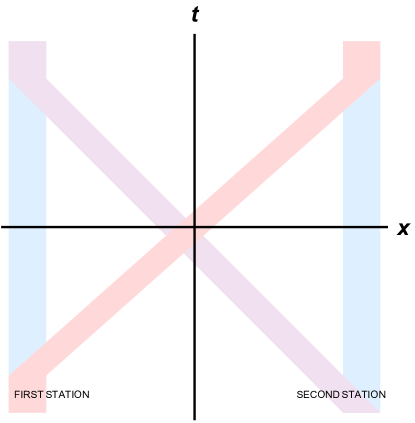
Figure 1: The motion is described by a two-dimensional region between the world lines.

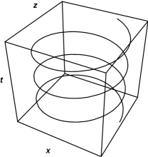
Figure 2: The helix, 3D parametric plot of the uniformly accelerated spatially circular worldline.

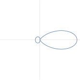
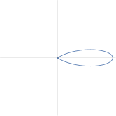
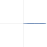
Figure 2: Synchrotron Angular Distribution; A polar plot with $\beta=0,0.33,$ $0.66,0.99$. The vertical axes is $x$ and the horizontal axis is $z$. The electron moves forward in a circle toward the horizontal $z$ axis. Notice each graph is a different worldline as the shape remains the same along a constant $v$ stationary worldline.

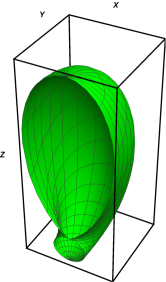
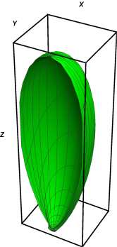
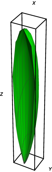
Figure 2: Synchrotron Angular Distribution in 3D; A spherical 3D plot with $\beta=0.3,$ $0.6,0.9$. The electron moves in the $z$ direction, but around the $x$ axis in circular motion. The plot range is $\theta=[0,\pi]$ and $\phi=[0,\pi]$.

Each observer can measure the time of events on his own world line. The observer cannot directly measure the time of an event outside of its world line. Suppose observer $1$ sends a signal to observer $2$ at the time of $t_{1}$, then he send a signal back Fig. (2). As result we can formulate three possibilities:

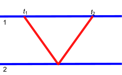
Figure 2: Signal exchange between observers.

• In case when $t_{2}<t_{1}$, the response signal comes before sending the first signal. But, this opportunity is impossible.

• When $t_{2}-t_{1}$ is positive, the difference can be very small. In this situation, we can introduce the absolute time, which the same for all observers. Before creating the theory of relativity, everyone thought like this.

• In the last case when $t_{2}-t_{1}$ can not be smaller than some positive value and it is the fastest signal. And this is true for the real world.

Such the fastest signal can be only light. Because photons are massless particle. For example, we will image that event $O$ be a explosion. The first thing that observer will see is the flash (light). On the world line light emitted at $O$ form the light half-cones of the future and past of this event. These area of space – time is called the future and past of $O$. Events inside and on the border of these half-cones can affect on the $O$ event. The region outside the light cones is in the elsewhere of $O$. Events in this area can not affect $O$, and they can not influence to them.

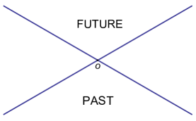
Figure 3: Past and Future events of $O$.

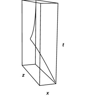
Figure 3: The cusp world line which is spatially a semi-cubic parabola plotted in a 3D parametric plot.

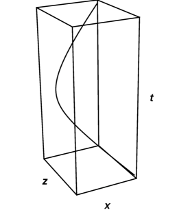
Figure 4: The infrator worldline (spatial catenary) plotted in a 3D parametric plot.

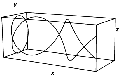
Figure 4: Spatial Projection of the Hypertorsional worldline with $\tau=10$, $\nu=\kappa=1$. Proper time ranges from $-1$ to $1$.

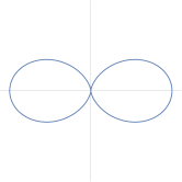
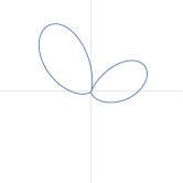
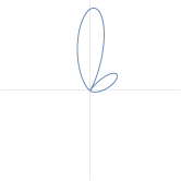
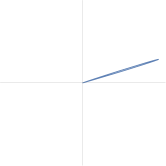
Figure 3: Cusp Angular Distribution; A polar plot with $\beta=0.0,0.333,$ $0.666,0.999$. The vertical axes is $x$ and the horizontal axis is $z$. The electron moves in both dimensions.

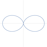
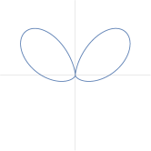
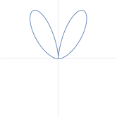
Figure 4: Catenary Angular Distribution; The catenary hangs as a chain would with the vertical axis $x$ and horizontal axis as $z$. A polar plot with $v_{R}=0.0001$ and $\beta=0.001,0.333,$ $0.665,0.997$. The electron moves in both dimensions but at high speeds moves mostly in the $x$-direction (thus the reason for the beaming in the $x$-direction).

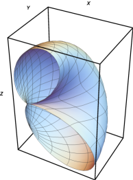
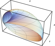
Figure 3: Cusp Angular Distribution; A polar plot with $\beta=0.3,$ $0.6,0.9$. The electron moves between $x$ and $z$ dimensions,directed as resulting vector. The plot range is $\theta=[0,\pi]$ and $\phi=[0,\pi]$.

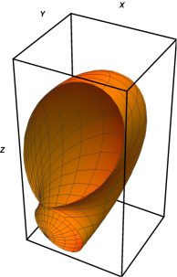
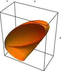
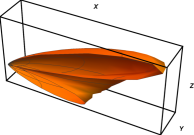
Figure 4: Catenary Angular Distribution; Additional torsion is added with substantial Rindler drift: $v_{R}=0.2$. Here $\beta=0.3,$ $0.6,0.9$ . Direction of electron appear as resulting vector from components along $x$ and $z$ dimensions. The plot range is $\theta=[0,\pi]$ and $\phi=[0,\pi]$.

The light cone in three dimensional space – time is shown in the Fig. (4) with two space coordinates and one time coordinate. The light cone in two dimensional space – time is shown in the Fig. (3) with one space and one time coordinate. The future events are inside the light of the semi-cone of the future, also the past events are inside the light half-cone of the past, while elsewhere events - outside the light cone.

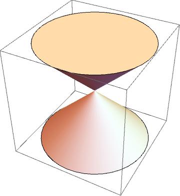
Figure 4: Light cone in 3D space – time.

2 Lorentz transformation

An object moves by inertia when no forces act on it. By Galileo’s principle of relativity, all inertial observers are equal. If one inertial observer did some experiment and got some result, and the other inertial observer who did the same experiment get the same result.

Figure 5: Two inertial observers.

If two inertial observers passed each other, and observer $1$ sent a light signal at time $t_{1}$ and the observer $2$ received it at the moment $t_{2}$ then we can write:

$$t_{2}=t_{1}e^{\phi},$$ (1)

where $\phi$ is the angle between the world lines of observers $1$ and $2$.

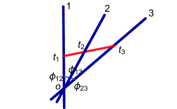
Figure 6: Three inertial observers in the same plane.

Consider three inertial observers moving in the same plane. Let their world lines intersect at point $O$. Then:

$$t_{2}=t_{1}e^{\phi_{12}},\;\;\;t_{3}=t_{1}e^{\phi_{13}}=t_{2}e^{\phi_{23}},$$ (2)

$$\phi_{13}=\phi_{12}+\phi_{23},$$ (3)

as in Euclidean geometry. The addition of angles is true only for world lines in one plane.

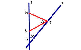
Figure 7: Signal exchange between two inertial observers.

Now let the observer $1$ send a light signal at the moment $t_{1}$ and the observer $2$ receives it at $t$ in event $A$ Fig. (7), and send a response signal. The observer $1$ receives it at the moment $t_{2}$. As we know, $t=t_{1}e^{\phi}$ ; besides, $t_{2}$ = $te^{\phi}$, then we get

$$t_{1}=te^{-\phi},\;\;\;\;\;\;t_{2}=te^{\phi}.$$ (4)

If event $A$ occurred outside the world line of observer $1$, so observer cannot measure the time . It is better to find the time of event $A$ from the point of view of observer $1$ in the interval $[t_{1},t_{2}]$, since the light signal propagates in both directions equally. Similarly we find the coordinate of the event $A$ from the view of the observer $1$ as half of this time interval. Thus, the time and space coordinates of the event $A$ from the point of view of the observer $1$ are

$$x^{0}=\frac{t_{1}+t_{2}}{2},\;\;\;\;\;\;x^{1}=\frac{t_{2}-t_{1}}{2}.$$ (5)

By substituting Eq. (2.4), we get

$$x^{0}=t\cosh{\phi},\;\;\;\;\;\;x^{1}=t\sinh{\phi}.$$ (6)

We found very important result for defining the magnitude

$$x^{2}=(x^{0})^{2}-(x^{1})^{2}=t^{2}.$$ (7)

and it does not depend on how the observer $1$ moves . The components of the $x^{0}$, $x^{1}$ from point $O$ to point $A$ are different for each observer. The invariant quantity $x^{2}$ is the square of the distance from $O$ to $A$ and it is equal to square of $t$, according to the observer $2$ . Also compared to the usual Euclidean calculation there is difference in sign. Instead of the plus sign between two members there is a minus sign. For this reason, the space – time geometry is called pseudo-Euclidean or Minkowski geometry. It can be seen from Eq. (6), where usual Newtonian velocity of the observer $2$ with respect to the observer $1$ is equal to

$$u=\frac{x^{1}}{x^{0}}=\tanh{\phi}$$ (8)

where $u<1$, and tends to $1$ when $\phi\to\infty$. But it is more convenient to use the angle $\phi$ between the world lines.

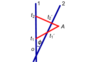
Figure 8: Lorentz transformation.

In the Fig.(8) it is shown how are the coordinates of $x^{0}$, $x^{1}$ of events $A$ related to the observer $1$ and the coordinates $x^{0}$’, $x^{1}$’ of the same event from the view of the observer $2$.

$$x^{\prime 0}=\frac{t_{1}^{\prime}+t_{2}^{\prime}}{2},\;x^{\prime 1}=\frac{t_{2}^{\prime}-t_{1}^{\prime}}{2},$$ (9)

where

$$t_{1}^{\prime}=t_{1}e^{\phi},\;\;\;\;\;\;t_{2}^{\prime}=t_{2}e^{-\phi}.$$ (10)

The final step involves the substitution of:

$$t_{1}=x^{0}-x^{1},\;\;\;\;\;\;t_{2}=x^{0}+x^{1}.$$ (11)

This will finally give us our answer,

$$x^{\prime 0}=x^{0}\cosh\phi-x^{1}\sinh\phi,\quad x^{\prime 1}=-x^{0}\sinh\phi+x^{1}\cosh\phi,$$ (12)

which is the well-known Lorentz transformation.

3 Geometry of Minkowski

Lets consider the vector $x$ from points $O$ to point $A$ Fig. (4). Logically, we can conclude the 3 possibilities:

• $x^{2}>0$ is a timelike vector and it can be directed to the future or to the past. By Lorentz transformation, we can ensure that component $x^{0}$ is nonzero and others are zero .

• $x^{2}=0$ is a light-like vector, which $A$ lies on the light cone of event $O$, directed along the light cone. Two light-like vectors cannot be compared (which is longer and shorter), except when they are collinear.

• $x^{2}<0$ is a space-like vector. By Lorentz transformation, we can find that the only nonzero component is $x^{1}$ (when the $O$ and $A$ events occur simultaneously).

Previously we described the vector $x^{2}$. And now lets make the scalar product of two vectors ($x\cdot y$),

$$x\cdot y=\frac{(x+y)^{2}-x^{2}-y^{2}}{2}=x^{0}y^{0}-x^{1}y^{1}.$$ (13)

In the four-dimensional space – time $x\cdot y=x^{0}y^{0}-x^{1}y^{1}-x^{2}y^{2}-x^{3}y^{3}$. Beside the contravariant components $x^{\mu}$ of the vector $x(\mu=0,1,2,3)$, we introduce covariant components $x^{\mu}$:

$$x_{0}=x^{0},\;\;\;x_{1}=-x^{1},\;\;\;x_{2}=-x^{2},\;\;\;x_{3}=-x^{3}.$$ (14)

Then the dot product has a simple form:

$$x\cdot y=x^{\mu}y_{\mu}=x_{\mu}y^{\mu},$$ (15)

where the index on top and on the bottom means the summation from 0 to 3. The vectors $x$ and $y$ are orthogonal if there scalar product equal to zero ($x\cdot y=0$).

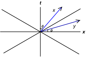
Figure 9: Orthogonal vectors.

Two timelike vectors can not be orthogonal to each other. If both have same direction to the future or past their scalar product is greater than zero. If one have direction to the future and another to the past their scalar product is less than zero. The timelike vector $x$ is orthogonal to the space vector $y$, if their directions are symmetrical to each other with respect to the light-like straight line Fig. (9). Orthogonality is not violated if $y$ is multiplied by a scalar. Two space-like vectors can be orthogonal to each other, if the plane is space-like, then its geometry is Euclidean, and these two vectors can be orthogonal. A timelike vector $x$ of length $t$ ($x^{2}=t^{2}$), with angle $\phi$ directed to the time axis, has the components $x^{\mu}=t(\cosh\phi,\sinh\phi)$ Fig. (10). Its projection in the direction $e^{\mu}=(1,0)$ equal to $t\cosh\nu$. It is always greater or equal to $t$, its equal when $\phi=0$.

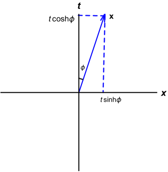
Figure 10: The projections of the timelike vector $x$ on the coordinate axis.

4 Four-velocity and four-acceleration

The main description for this section was taken from Rindler’s book [Rindler:1960zz]. When we consider motion along timelike directions we often work with the invariant:

$$d\tau^{2}=\frac{ds^{2}}{c^{2}}=dt^{2}-\frac{dx^{2}+dy^{2}+dz^{2}}{c^{2}}$$ (16)

where $d\tau$ is a interval of proper time. Otherwise, we can write speed of the particle as $v$, then we have from Eq.(16):

$$\frac{d\tau^{2}}{dt^{2}}=1-\frac{v^{2}}{c^{2}},\;\;\;\frac{dt}{d\tau}=\left(1-\frac{v^{2}}{c^{2}}\right)^{-1/2}=\gamma.$$ (17)

Lets now consider four-vector motion with worldline $x^{\mu}=x^{\mu}(\tau)$. We denote vectors $v^{\mu}$ and $a^{\mu}$ as four-velocity and four-acceleration respectively:

$$v^{\mu}=\frac{dx^{\mu}}{d\tau},\;\;\;\;\;\;a^{\mu}=\frac{d^{2}x^{\mu}}{d\tau^{2}}=\frac{dv^{\mu}}{d\tau}.$$ (18)

From Eq.(17) we find that:

$$v^{\mu}=\frac{dx^{\mu}}{d\tau}=\frac{dx^{\mu}}{dt}\frac{dt}{d\tau}=\gamma\frac{dx^{\mu}}{dt},$$ (19)

and

$$a^{\mu}=\frac{dv^{\mu}}{d\tau}=\gamma\frac{dv^{\mu}}{dt}.$$ (20)

The relation between the tree vector acceleration $a$ and four acceleration $a^{\mu}$ can be written

$$a^{\mu}=\frac{dv^{\mu}}{d\tau}=\gamma\frac{dv^{\mu}}{dt}=\gamma\frac{d}{dt}(\gamma c,\gamma v)=\gamma\left(\frac{d\gamma}{dt}c,\frac{d\gamma}{dt}v+\gamma a\right),$$ (21)

and proper time is

$$a_{\mu}a^{\mu}=-\alpha^{2}.$$ (22)

From equation above we have:

$$a_{\mu}a^{\mu}=\gamma^{2}[\dot{\gamma}^{2}c^{2}-(\dot{\gamma}v+\gamma a)^{2}],$$ (23)

where $\gamma=\gamma(v)$. Using the relation $\dot{\gamma}=\gamma^{3}v\dot{v}/c^{2}$ and three vector results like $(v^{\mu})^{2}=v^{2}$ we find :

$$\alpha^{2}=-a_{\mu}a^{\mu}=\gamma^{2}[\dot{\gamma}^{2}v^{2}+2\gamma\dot{\gamma}v\dot{v}+\gamma^{2}a^{2}-\dot{\gamma}^{2}c^{2}]=\gamma^{6}v^{2}\dot{v}^{2}/c^{2}+\gamma^{4}a^{2}.$$ (24)

In an inertial frame in which the object is at the rest, the 3-vector acceleration, combined with the zero time component, 4-object acceleration occurs, which makes it its own Lorentz-invariant acceleration. Thus, the concept is useful in the following cases: (i) with accelerated coordinates, (ii) at relativistic speeds and (iii) in curved spacetime.

In the unidirectional case where the acceleration of an object is parallel or antiparallel to its velocity to observer, the proper acceleration $\alpha$ and the acceleration of coordinates $a$ are connected through the Lorentz factor $\gamma$ for $\alpha=\gamma^{3}a$. Therefore, the change in the proper velocity $w=dx/d\tau$ is the integral of the proper acceleration with respect to the time of the stationary system $t$, that is, $\Delta w=\alpha\Delta t$ for the constant $\alpha$. At low speeds, this comes down to relationship between the coordinate velocity and the time of coordinate acceleration, that is, $\Delta v=a\Delta t$.

For constant unidirectional proper acceleration, there are similar relations between the rapidity $\eta$ and the elapsed proper time $\Delta\tau$, as well as between the Lorentz coefficient $\gamma$ and the distance $\Delta x$. Namely:

$$\alpha=\frac{\Delta w}{\Delta t}=c\frac{\Delta\eta}{\Delta\tau}=c^{2}\frac{\Delta\gamma}{\Delta x},$$ (25)

where different velocity parameters are related by

$$\eta=\sinh^{-1}(\frac{w}{c})=\tanh^{-1}(\frac{v}{c})=\pm\cosh^{-1}(\gamma).$$ (26)

These equations illustrate some of the useful parameters of accelerated motion at high speed.

5 Covariant Power

Using the the relativistic covariant form of Larmor’s formula, an accelerated point charge has power,

$$P=\frac{2}{3}q^{2}\alpha^{2},$$ (27)

where $\alpha$ is the proper acceleration (as we will see in Eq. (30)) and $q$ is the charge. A constant proper acceleration yields constant power. The proper acceleration is the scalar invariant magnitude

$$\alpha^{2}\equiv-a_{\mu}a^{\mu},$$ (28)

of the four-acceleration $a^{\mu}$,

$$a^{\mu}=\frac{d^{2}x^{\mu}}{d\tau^{2}},$$ (29)

most easily expressed (see e.g. [Rindler:1960zz, Proceedings]), in two nice forms:

$$\alpha^{2} = \gamma^{4}a^{2}+\gamma^{6}(\boldsymbol{v}\cdot\boldsymbol{a})^{2},$$ (30)

$$= \gamma^{6}a^{2}-\gamma^{6}(\boldsymbol{v}\times\boldsymbol{a})^{2}\;.$$ (31)

In the case of straight-line motion, parallel vectors $\boldsymbol{v}\times\boldsymbol{a}=\boldsymbol{0}$ yield $\alpha^{2}=\gamma^{6}a^{2}$. In the case of circular motion, the three-acceleration vector is perpendicular to the three-velocity vector, $\boldsymbol{v}\cdot\boldsymbol{a}=0$, and one obtains $\alpha^{2}=\gamma^{4}a^{2}$. The acceleration ratio, $A_{\textrm{WL}}\equiv\alpha^{2}/a^{2}$, is given for each worldline in Appendix 8.

In the instantaneous rest frame of the accelerating particle, the proper acceleration, $\alpha$, is the acceleration as measured by a hand-held accelerometer. It is what is ‘felt’ and is the property of the particle, a Lorentz scalar invariant in all frames. For a stationary worldline the Lorentz scalar remains constant and the proper acceleration, $\alpha=\kappa$ is the curvature, the simplest of the curvature invariants for stationary worldlines (the others being torsion, $\tau$, and hypertorsion, $\nu$ [Letaw:1980yv]). The power is consequently,

$$P=\frac{2}{3}q^{2}\kappa^{2}.$$ (32)

Chapter 2 Stationary Worldlines

1 Nulltor

The Nulltor is a linear motion at the world line in 4-dimensional space-time. Parameters of the particle which moves along this trajectory can be described through hyperbolic functions :

$$x^{\mu}(s)=\kappa^{-1}\left(\sinh(\kappa s),0,0,\cosh(\kappa s)\right).$$ (1)

where $s$ is a proper time. The four-dimensional velocity vector is a time like vector and lies inside the light cone. Due to derivation along time we can find three components of velocities on the $x,y$ and $z$ axis:

$$v_{x} = \frac{ds}{dt}\frac{dx}{ds}=0,$$ (2)

$$v_{y} = 0,$$ (3)

$$v_{z} = \frac{ds}{dt}\frac{dz}{ds}=\tanh{(\kappa s)},$$ (4)

and total velocity is:

$$v^{2}=v_{x}^{2}+v_{y}^{2}+v_{z}^{2}=\tanh^{2}{(\kappa s)}.$$ (5)

Three dimensional acceleration components could be found also through derivation of velocity :

$$a_{x} = \frac{ds}{dt}\frac{dv_{x}}{ds}=0\,,$$ (6)

$$a_{y} = 0,$$ (7)

$$a_{z} = \frac{ds}{dt}\frac{dv_{z}}{ds}=\kappa\sech^{3}(\kappa s).$$ (8)

and total acceleration is:

$$a^{2}=a_{x}^{2}+a_{y}^{2}+a_{z}^{2}=\kappa^{2}\sech^{6}(\kappa s).$$ (9)

Proper time $s$ can described by $\gamma$ through equation :

$$1-\gamma^{-2} = \tanh^{2}{(\kappa s)},$$ (10)

here we substitute total velocity Eq. (5) with $\beta$ function which can be described through $\gamma$. Finally we will get:

$$s = \sqrt{\frac{1}{\kappa}\arctan(1-\gamma^{-2})}.$$ (11)

Due to expression above we can find more shorter description of velocity and acceleration, like in Appendix 10.

2 Ultrator

Synchrotron radiation , also can be called Ultrator motion, is electromagnetic radiation and evaporated by charged particle. Synchrotron radiation moving with relativistic speed along circular trajectory and bent by a magnetic field. Parametric representation of synchrotron radiation :

$$x^{\mu}(s)=\rho^{-2}\left(\tau\,\rho\,s,\kappa\cos\rho s,0,\kappa\sin\rho s\right).$$ (12)

where $\rho^{2}=\tau^{2}-\kappa^{2}$ . Velocity components in three dimensional space:

$$v_{x} = \frac{ds}{dt}\frac{dx}{ds}=-\frac{\kappa\sin(\rho s)}{\tau},$$ (13)

$$v_{y} = 0,$$ (14)

$$v_{z} = \frac{ds}{dt}\frac{dz}{ds}=\frac{\kappa\cos(\rho s)}{\tau},$$ (15)

$$v^{2}=v_{x}^{2}+v_{y}^{2}+v_{z}^{2}=\frac{\kappa^{2}}{\tau^{2}}.$$ (16)

Components of the acceleration:

$$a_{x} = \frac{ds}{dt}\frac{dv_{x}}{ds}=-\frac{\kappa\rho^{2}\sin(\rho s)}{\tau^{2}},$$ (17)

$$a_{y} = 0,$$ (18)

$$a_{z} = \frac{ds}{dt}\frac{dv_{z}}{ds}=-\frac{\kappa\rho^{2}\cos(\rho s)}{\tau^{2}}.$$ (19)

Total acceleration we find us:

$$a^{2}=a_{x}^{2}+a_{y}^{2}+a_{z}^{2}=\frac{\kappa^{2}\rho^{4}}{\tau^{4}}.$$ (20)

Also we can find expression of $\gamma$ in terms of $\kappa$ and $\tau$:

$$\gamma=\frac{1}{\sqrt{1-\frac{\kappa^{2}}{\tau^{2}}}}.$$ (21)

In Appendix 10 it is shown components of velocity and acceleration , in case when proper time is zero.

3 Parator

Here we consider a parator motion which moves along the cusp trajectory. Cusp - a singular point at which the curved line is divided into two branches that have the same direction vector at this point. That is, the branches at a given point have a common tangent and the movement along them initially occurs in the same direction. Parametric representation of cusp motion in flat space:

$$x^{\mu}(s)=\left(s+\frac{1}{6}\kappa^{2}s^{3},\frac{1}{2}\kappa s^{2},0,\frac{1}{6}\kappa^{2}s^{3}\right).$$ (22)

Derivation of the velocity components in three dimensional space:

$$v_{x} = \frac{ds}{dt}\frac{dx}{ds}=\frac{2\kappa s}{\kappa^{2}s^{2}+2},$$ (23)

$$v_{y} = 0,$$ (24)

$$v_{z} = \frac{ds}{dt}\frac{dz}{ds}=\frac{\kappa^{2}s^{2}}{\kappa^{2}s^{2}+2}.$$ (25)

This gives total velocity:

$$v^{2}=v_{x}^{2}+v_{y}^{2}+v_{z}^{2}=\frac{\kappa^{2}\tau^{2}\left(\kappa^{2}\tau^{2}+4\right)}{\left(\kappa^{2}\tau^{2}+2\right)^{2}}\;.$$ (26)

Further we examine the components of the acceleration at the same way,

$$a_{x} = \frac{ds}{dt}\frac{dv_{x}}{ds}=\frac{8\kappa-4\kappa^{3}\tau^{2}}{\left(\kappa^{2}\tau^{2}+2\right)^{3}}\,,$$ (27)

$$a_{y} = 0,$$ (28)

$$a_{z} = \frac{ds}{dt}\frac{dv_{z}}{ds}=\frac{8\kappa^{2}\tau}{\left(\kappa^{2}\tau^{2}+2\right)^{3}}.$$ (29)

The vector summation gives us:

$$a^{2}=a_{x}^{2}+a_{y}^{2}+a_{z}^{2}=\frac{16\kappa^{2}\left(\kappa^{4}\tau^{4}+4\right)}{\left(\kappa^{2}\tau^{2}+2\right)^{6}}.$$ (30)

Through Eq. (30) we can find relation of the proper time as $s=s(\gamma)$:

$$\gamma=1+\frac{\kappa^{2}\tau^{2}}{2}\quad\Leftrightarrow\quad\tau=\kappa^{-1}\sqrt{2\gamma-2},$$ (31)

obtained by adding Eq. (26) into the $\gamma$ definition.

Finally, we can describe velocity and acceleration components in more convenient way, through relation between $\gamma$ and curvature invariants $\kappa$ and $\tau$, as it is shown in Appendix 10.

4 Infrator

In this section we consider Infrator motion , which has a trajectory of curved chain and also can be called catenary motion. Catenary is a line, the shape of which takes a flexible homogeneous chain (hence the name) with fixed ends in a uniform gravitational field. In geometry, the catenary is the graph of the hyperbolic cosine function. Parametric representation of catenary or infrator motion :

$$x^{\mu}(s)=\sigma^{-2}\left(\kappa\sinh(s\sigma),\kappa\cosh(s\sigma),0,s\tau\sigma\right).$$ (32)

where $\sigma^{2}=\kappa^{2}-\tau^{2}$.Derivation of the velocity in 3-dimensional space:

$$v_{x} = \frac{ds}{dt}\frac{dx}{ds}=\tanh(s\sigma),$$ (33)

$$v_{y} = 0\;,$$ (34)

$$v_{z} = \frac{ds}{dt}\frac{dz}{ds}=v_{R}\;\text{sech}(s\sigma),$$ (35)

where $v_{R}=\frac{\tau}{\kappa}$ is minimum velocity. Then total velocity :

$$v^{2}=v_{x}^{2}+v_{y}^{2}+v_{z}^{2}=\frac{\tau^{2}\text{sech}^{2}(s\sigma)}{\kappa^{2}}+\tanh^{2}(s\sigma).$$ (36)

Further we derive the components of the acceleration :

$$a_{x} = \frac{ds}{dt}\frac{dv_{x}}{ds}=\frac{\sigma^{2}}{\kappa}\text{sech}^{3}(s\sigma),$$ (37)

$$a_{y} = 0,$$ (38)

$$a_{z} = \frac{ds}{dt}\frac{dv_{z}}{ds}=-\frac{\sigma^{2}\tau}{\kappa^{2}}\tanh(s\sigma)\text{sech}^{2}(s\sigma).$$ (39)

Sum of the vectors give us:

$$a^{2}=a_{x}^{2}+a_{y}^{2}+a_{z}^{2}=\frac{\sigma^{4}\tau^{2}\tanh^{2}(s\sigma)\text{sech}^{4}(s\sigma)}{\kappa^{4}}+\frac{\sigma^{4}\text{sech}^{6}(s\sigma)}{\kappa^{2}}.$$ (40)

If substitute total velocity with $\beta$ function we can find expression of proper time:

$$1-\gamma^{-2} = \frac{\tau^{2}\text{sech}^{2}(s\sigma)}{\kappa^{2}}+\tanh^{2}(s\sigma),$$ (41)

where proper time $s$ :

$$s = \frac{1}{2\sigma}\textrm{ln}\left(2\frac{\gamma^{2}}{\gamma_{R}^{2}}-2\frac{\gamma}{\gamma_{R}}\sqrt{\frac{\gamma^{2}}{\gamma_{R}^{2}}-1}-1\right),$$ (42)

where $\gamma_{R}^{-1}=\sqrt{1-v_{R}^{2}}$. Finally, we can rewrite equation of total acceleration in more convenient way :

$$a = \frac{\sqrt{\gamma^{2}\tau^{2}+\kappa^{2}}}{\gamma^{3}}.$$ (43)

5 Hypertor

The hypertor motion is a superposition of a uniform synchrotron motion and a constant linear motion, ultimately forming a spiral trajectory. The path of particle which moving along this world line has a helix form with slope that decrease to zero when its proper time equal to zero and increase when proper time grows. The hypertor motion is specified in world line coordinates by parametric equations of the form:

$$x^{\mu}(s)=\left(\frac{\Delta}{RR_{+}}\sinh(R_{+}s),\,\frac{\Delta}{RR_{+}}\cosh(R_{+}s),\right.\\ \left.\frac{\kappa\tau}{R\Delta R_{-}}\cos(R_{-}s),\,\frac{\kappa\tau}{R\Delta R_{-}}\sin(R_{-}s)\right),$$ (44)

where all constants are the combination of three invariant variables:

$$\Delta^{2}\equiv\frac{1}{2}(R^{2}+\kappa^{2}+\tau^{2}+\nu^{2})\,\,,$$

$$R^{2}\equiv R_{+}^{2}+R_{-}^{2}\,\,,$$

$$R_{\pm}^{2}\equiv{\sqrt{a^{2}+b^{2}}\pm a}\,\,,$$

$$a=\frac{1}{2}\left(\kappa^{2}-\nu^{2}-\tau^{2}\right)\,\,,\qquad b=\kappa\nu\,.$$

Here we find the velocity of Hypertor in three coordinates as well as others:

$$v_{x} = \frac{ds}{dt}\frac{dx}{ds}=\tanh\left(R_{+}s\right),$$ (45)

$$v_{y} = \frac{ds}{dt}\frac{dx}{ds}=v_{\textrm{min}}\sin\left(R_{-}s\right)\text{sech}\left(R_{+}s\right)\;,$$ (46)

$$v_{z} = \frac{ds}{dt}\frac{dz}{ds}=v_{\textrm{min}}\cos\left(R_{-}s\right)\text{sech}\left(R_{+}s\right).$$ (47)

where $v_{\textrm{min}}=\frac{\kappa\tau}{\Delta^{2}}$ is a minimum velocity,

$$v^{2}=v_{x}^{2}+v_{y}^{2}+v_{z}^{2}=1-\frac{\text{sech}^{2}(R_{+}s)}{\gamma_{\textrm{min}}^{2}},$$ (48)

where $\gamma_{\textrm{min}}^{-1}=\sqrt{1-v_{\textrm{min}}^{2}}$. Further we take derivation again and find acceleration :

$$a_{x}=\frac{RR_{+}}{\Delta}\text{sech}^{3}(R_{+}s),$$ (49)

$$a_{y}=\frac{Rv_{\textrm{min}}}{\Delta}\text{sech}^{2}(R_{+}s)[R_{+}\sin(R_{-}s)\tanh(R_{+}s)-R_{-}\cos(R_{-}s)],$$ (50)

$$a_{z}=-\frac{Rv_{\textrm{min}}}{\Delta}\text{sech}^{2}(R_{+}s)[R_{+}\cos(R_{-}s)\tanh(R_{+}s)+R_{-}\sin(R_{-}s)],$$ (51)

$$a^{2}=a_{x}^{2}+a_{y}^{2}+a_{z}^{2}=\frac{R^{2}\text{sech}^{4}(R_{+}s)}{\Delta^{2}}\left(R^{2}v_{\textrm{min}}^{2}+R_{+}^{2}\frac{\text{sech}^{2}(R_{+}s)}{\gamma_{\textrm{min}}^{2}}\right).$$ (52)

Then substitute total velocity with $\beta$ and find proper time :

$$1-\gamma^{-2}=1-\frac{\text{sech}^{2}(R_{+}s)}{\gamma_{\textrm{min}}^{2}},$$ (53)

where proper time $s$ :

$$s=-\frac{1}{R_{+}}\cosh^{-1}\left(\frac{\gamma}{\gamma_{\textrm{min}}}\right),$$ (54)

and we can also rewrite acceleration components:

$$a^{2}=\frac{\gamma_{\min}^{4}}{\gamma^{4}\Delta^{2}}\left(R^{4}v_{\min}^{2}+\frac{R^{2}R_{+}^{2}}{\gamma^{2}}\right).$$ (55)

Vacuum Spectra

Stationary world lines are special in part because each have a unique spectrum, e.g. Parator is exactly calculable and distinctly non-Planckian. Each unique motion is a stationary world line solution of the Frenet equations when the curvature invariants of proper acceleration and proper angular velocity are constant. There is a dearth of papers that have treated these worldlines over the last four decades, for instance the exactly solvable motion has been treated in only a handful of papers: [Rosu:1999ad, Padmanabhan:1983ub, Takagi:1986kn, Audretsch:1995iw, Sriramkumar:1999nw, Leinaas:2000mh, Rosu:2005iu, Louko:2006zv, Obadia:2007qf, Russo:2009yd].

As an illustration of the importance of investigating these worldlines, it is good to remark that the vacuum spectra differ among the stationary worldlines. For instance, two can be calculated exactly: the Nulltor and Parator motions which are both one parameter motions ($\kappa$ only). The vacuuum fluctuation spectrum for the zero torsion case [Letaw:1980yv], is the same Planckian distribution as found by Unruh [Unruh:1976db] for uniform acceleration radiation, and scales (with $\omega/\kappa\gg 1$):

$$\frac{1}{e^{2\pi\omega/\kappa}-1}\approx e^{-2\pi\omega/\kappa},\quad\textrm{with}\quad T=\frac{\kappa}{2\pi}=0.159\kappa.$$ (56)

The spectrum for the paratorsional worldline is Letawian, with a hotter temperature (by a factor of $\pi/\sqrt{3}=1.81$), scaling:

$$e^{-\sqrt{12}\omega/\kappa},\quad\textrm{with}\quad T=\frac{\kappa}{\sqrt{12}}=0.289\kappa.$$ (57)

The Nulltor and Parator cases both have uniform acceleration of $\kappa$, with an exactly analytic spectrum, recently confirmed in [Proceedings].

Chapter 3 Calculating the Power Distribution

1 Lienard-Wiechert Potentials

In order to correctly calculate the power distribution, we must take into account the relativistic effects of a point charge in a field. In this section, we will find the potentials for moving a point charge, and then in the following sections we will find the electric and magnetic fields, where we will use them to find the angular distribution and finally the power distribution.Also we will do all our calculation in natural units, then we must remember that $c=1,\epsilon_{0}=1/4\pi,\mu_{0}=4\pi$, where $c$ is the speed of light, $\epsilon_{0}$ and $\mu_{0}$ is a electric and magnetic constants respectively. Further we will consider moving particle in the radiated sphere . Lets firstly specified trajectory,

$$\boldsymbol{w}(t)=\textrm{position of }q\textrm{ at time }t.$$ (1)

The retarded time (time that take a particle to move from the center) can be found by the equation

$$|\boldsymbol{r}-\boldsymbol{w}(t)|=t-t_{r},$$ (2)

where the left side is the distance that radiation travel and right side is the time it takes to it. We call $\boldsymbol{w}(t)$ as the retarded position of the particle, then is the vector from retarded position to the field point $\boldsymbol{r}$:

$${\mbox{$\leavevmode\resizebox{6.50403pt}{5.78172pt}{\includegraphics[trim=10.00002pt 0.0pt 140.00021pt 0.0pt,clip]{BoldR}}$}}=\boldsymbol{r}-\boldsymbol{w}(t).$$ (3)

Now, we can write basic potential equation like:

$$V(\boldsymbol{r},t)=\int\frac{\rho(\boldsymbol{r^{\prime}},t_{r})}{{\mbox{$\leavevmode\resizebox{6.50403pt}{5.78172pt}{\includegraphics[trim=10.00002pt 0.0pt 140.00021pt 0.0pt,clip]{ScriptR}}$}}}d\tau^{\prime}$$ (4)

where $\rho$ and $\tau^{\prime}$ is a density and volume respectively. We can suggest that retarded potential of point charge is

$$V(\boldsymbol{r},t)=\frac{q}{{\mbox{$\leavevmode\resizebox{6.50403pt}{5.78172pt}{\includegraphics[trim=10.00002pt 0.0pt 140.00021pt 0.0pt,clip]{ScriptR}}$}}}.$$

However it is not true, because it did not account relativistic effect. It is true that comes outside the integral, but charge not equal to:

$$q=\int\rho(\boldsymbol{r^{\prime}},t_{r})d\tau^{\prime}.$$ (5)

Here we must remember about retarded time ($t_{r}=t-{\mbox{$\leavevmode\resizebox{6.50403pt}{5.78172pt}{\includegraphics[trim=10.00002pt 0.0pt 140.00021pt 0.0pt,clip]{ScriptR}}$}}$), and for extended particle the retardation will be written with factor $(1-\hat{{\mbox{$\leavevmode\resizebox{6.50403pt}{5.78172pt}{\includegraphics[trim=10.00002pt 0.0pt 140.00021pt 0.0pt,clip]{BoldR}}$}}}\cdot\boldsymbol{v})^{-1}$, where $\boldsymbol{v}$ is the velocity of the charge:

$$\int\rho(\boldsymbol{r^{\prime}},t_{r})d\tau^{\prime}=\frac{q}{1-\hat{{\mbox{$\leavevmode\resizebox{6.50403pt}{5.78172pt}{\includegraphics[trim=10.00002pt 0.0pt 140.00021pt 0.0pt,clip]{BoldR}}$}}}\cdot\boldsymbol{v}},$$ (6)

where by extended we mean relativistic growth. For example when linear object become longer when in move faster or like in our case,

$$\tau^{\prime}=\frac{\tau}{1-\hat{{\mbox{$\leavevmode\resizebox{6.50403pt}{5.78172pt}{\includegraphics[trim=10.00002pt 0.0pt 140.00021pt 0.0pt,clip]{BoldR}}$}}}\cdot\boldsymbol{v}},$$ (7)

where $\tau$ is actual volume and $\tau^{\prime}$ is a apparent volume, and $\hat{{\mbox{$\leavevmode\resizebox{6.50403pt}{5.78172pt}{\includegraphics[trim=10.00002pt 0.0pt 140.00021pt 0.0pt,clip]{BoldR}}$}}}$ is a unit of vector from object to observer. Finally our potential will be :

$$V(\boldsymbol{r},t)=\frac{q}{{\mbox{$\leavevmode\resizebox{6.50403pt}{5.78172pt}{\includegraphics[trim=10.00002pt 0.0pt 140.00021pt 0.0pt,clip]{ScriptR}}$}}-{\mbox{$\leavevmode\resizebox{6.50403pt}{5.78172pt}{\includegraphics[trim=10.00002pt 0.0pt 140.00021pt 0.0pt,clip]{BoldR}}$}}\cdot\boldsymbol{v}}.$$ (8)

where ${\mbox{$\leavevmode\resizebox{6.50403pt}{5.78172pt}{\includegraphics[trim=10.00002pt 0.0pt 140.00021pt 0.0pt,clip]{BoldR}}$}}=\hat{{\mbox{$\leavevmode\resizebox{6.50403pt}{5.78172pt}{\includegraphics[trim=10.00002pt 0.0pt 140.00021pt 0.0pt,clip]{BoldR}}$}}}{\mbox{$\leavevmode\resizebox{6.50403pt}{5.78172pt}{\includegraphics[trim=10.00002pt 0.0pt 140.00021pt 0.0pt,clip]{ScriptR}}$}}$ is the vector from retarded position to the field point $\boldsymbol{r}$ and $\boldsymbol{v}$ is the velocity of charge at the retarded time. Also vector potential will be:

$$A(\boldsymbol{r},t)=\int\frac{\rho(\boldsymbol{r^{\prime}},t_{r})\boldsymbol{v}(t_{r})}{{\mbox{$\leavevmode\resizebox{6.50403pt}{5.78172pt}{\includegraphics[trim=10.00002pt 0.0pt 140.00021pt 0.0pt,clip]{ScriptR}}$}}}d\tau^{\prime}=\frac{\boldsymbol{v}}{{\mbox{$\leavevmode\resizebox{6.50403pt}{5.78172pt}{\includegraphics[trim=10.00002pt 0.0pt 140.00021pt 0.0pt,clip]{ScriptR}}$}}}\int\rho(\boldsymbol{r^{\prime}},t_{r})d\tau^{\prime},$$ (9)

or

$$A(\boldsymbol{r},t)=\frac{q\boldsymbol{v}}{{\mbox{$\leavevmode\resizebox{6.50403pt}{5.78172pt}{\includegraphics[trim=10.00002pt 0.0pt 140.00021pt 0.0pt,clip]{ScriptR}}$}}-{\mbox{$\leavevmode\resizebox{6.50403pt}{5.78172pt}{\includegraphics[trim=10.00002pt 0.0pt 140.00021pt 0.0pt,clip]{BoldR}}$}}\cdot\boldsymbol{v}}=\boldsymbol{v}V(\boldsymbol{r},t).$$ (10)

These equations are Lienard-Wiechert potentials for a moving point charge.

2 The field of a moving charge

To calculate the electric and magnetic fields of charge in natural units ($c=1,\epsilon_{0}=1/4\pi,\mu_{0}=4\pi$), we are use the Lienard-Wiechert potentials:

$$V(\boldsymbol{r},t)=\frac{q}{({\mbox{$\leavevmode\resizebox{6.50403pt}{5.78172pt}{\includegraphics[trim=10.00002pt 0.0pt 140.00021pt 0.0pt,clip]{ScriptR}}$}}-{\mbox{$\leavevmode\resizebox{6.50403pt}{5.78172pt}{\includegraphics[trim=10.00002pt 0.0pt 140.00021pt 0.0pt,clip]{BoldR}}$}}\cdot\boldsymbol{v})},\;\;\;\;\;\boldsymbol{A}(\boldsymbol{r},t)=v\;V(\boldsymbol{r},t),$$ (11)

and substitute them in Maxwell equations for electric and magnetic fields:

$$\boldsymbol{E}=-\nabla V-\frac{\partial\boldsymbol{A}}{\partial t},\;\;\;\;\;\boldsymbol{B}=\nabla\crossproduct\boldsymbol{A}.$$ (12)

Further we will use the equations like:

$${\mbox{$\leavevmode\resizebox{6.50403pt}{5.78172pt}{\includegraphics[trim=10.00002pt 0.0pt 140.00021pt 0.0pt,clip]{BoldR}}$}}=\boldsymbol{r}-\boldsymbol{w}(t_{r}),\;\;\textrm{and}\;\;\;\boldsymbol{v}=\boldsymbol{w}(t_{r}),$$ (13)

where $t_{r}$ is retarted time. We can write fuction of $\boldsymbol{r}$ and $t$ like:

$$|\boldsymbol{r}-\boldsymbol{w}(t_{r})|=t-t_{r}.$$ (14)

Firstly let’s start from gradient of potential $V$:

$$\nabla V=-\frac{q}{({\mbox{$\leavevmode\resizebox{6.50403pt}{5.78172pt}{\includegraphics[trim=10.00002pt 0.0pt 140.00021pt 0.0pt,clip]{ScriptR}}$}}-{\mbox{$\leavevmode\resizebox{6.50403pt}{5.78172pt}{\includegraphics[trim=10.00002pt 0.0pt 140.00021pt 0.0pt,clip]{BoldR}}$}}\cdot\boldsymbol{v})^{2}}\nabla({\mbox{$\leavevmode\resizebox{6.50403pt}{5.78172pt}{\includegraphics[trim=10.00002pt 0.0pt 140.00021pt 0.0pt,clip]{ScriptR}}$}}-{\mbox{$\leavevmode\resizebox{6.50403pt}{5.78172pt}{\includegraphics[trim=10.00002pt 0.0pt 140.00021pt 0.0pt,clip]{BoldR}}$}}\cdot\boldsymbol{v}).$$ (15)

By taking derivation of ${\mbox{$\leavevmode\resizebox{6.50403pt}{5.78172pt}{\includegraphics[trim=10.00002pt 0.0pt 140.00021pt 0.0pt,clip]{ScriptR}}$}}=t-t_{r}$,

$$\nabla{\mbox{$\leavevmode\resizebox{6.50403pt}{5.78172pt}{\includegraphics[trim=10.00002pt 0.0pt 140.00021pt 0.0pt,clip]{ScriptR}}$}}=-\nabla t_{r}.$$ (16)

Second term of product gives,

$$\nabla({\mbox{$\leavevmode\resizebox{6.50403pt}{5.78172pt}{\includegraphics[trim=10.00002pt 0.0pt 140.00021pt 0.0pt,clip]{BoldR}}$}}\cdot\boldsymbol{v})=({\mbox{$\leavevmode\resizebox{6.50403pt}{5.78172pt}{\includegraphics[trim=10.00002pt 0.0pt 140.00021pt 0.0pt,clip]{BoldR}}$}}\cdot\nabla)\boldsymbol{v}+(\boldsymbol{v}\cdot\nabla){\mbox{$\leavevmode\resizebox{6.50403pt}{5.78172pt}{\includegraphics[trim=10.00002pt 0.0pt 140.00021pt 0.0pt,clip]{BoldR}}$}}+{\mbox{$\leavevmode\resizebox{6.50403pt}{5.78172pt}{\includegraphics[trim=10.00002pt 0.0pt 140.00021pt 0.0pt,clip]{BoldR}}$}}\crossproduct(\nabla\crossproduct\boldsymbol{v})+\boldsymbol{v}\crossproduct(\nabla\crossproduct{\mbox{$\leavevmode\resizebox{6.50403pt}{5.78172pt}{\includegraphics[trim=10.00002pt 0.0pt 140.00021pt 0.0pt,clip]{BoldR}}$}}).$$ (17)

We will derive each term of Eq. (17) separately and add it together at the end. First term of Eq. (17) gives

$$({\mbox{$\leavevmode\resizebox{6.50403pt}{5.78172pt}{\includegraphics[trim=10.00002pt 0.0pt 140.00021pt 0.0pt,clip]{BoldR}}$}}\cdot\nabla)\boldsymbol{v}=\left({\mbox{$\leavevmode\resizebox{6.50403pt}{5.78172pt}{\includegraphics[trim=10.00002pt 0.0pt 140.00021pt 0.0pt,clip]{ScriptR}}$}}_{x}\frac{\partial}{\partial x}+{\mbox{$\leavevmode\resizebox{6.50403pt}{5.78172pt}{\includegraphics[trim=10.00002pt 0.0pt 140.00021pt 0.0pt,clip]{ScriptR}}$}}_{y}\frac{\partial}{\partial y}+{\mbox{$\leavevmode\resizebox{6.50403pt}{5.78172pt}{\includegraphics[trim=10.00002pt 0.0pt 140.00021pt 0.0pt,clip]{ScriptR}}$}}_{z}\frac{\partial}{\partial z}\right)\boldsymbol{v}(t_{r})=$$ (18)

$${\mbox{$\leavevmode\resizebox{6.50403pt}{5.78172pt}{\includegraphics[trim=10.00002pt 0.0pt 140.00021pt 0.0pt,clip]{ScriptR}}$}}_{x}\frac{d\boldsymbol{v}}{dt_{r}}\frac{\partial t_{r}}{\partial x}+{\mbox{$\leavevmode\resizebox{6.50403pt}{5.78172pt}{\includegraphics[trim=10.00002pt 0.0pt 140.00021pt 0.0pt,clip]{ScriptR}}$}}_{y}\frac{d\boldsymbol{v}}{dt_{r}}\frac{\partial t_{r}}{\partial y}+{\mbox{$\leavevmode\resizebox{6.50403pt}{5.78172pt}{\includegraphics[trim=10.00002pt 0.0pt 140.00021pt 0.0pt,clip]{ScriptR}}$}}_{z}\frac{d\boldsymbol{v}}{dt_{r}}\frac{\partial t_{r}}{\partial z}=\boldsymbol{a}({\mbox{$\leavevmode\resizebox{6.50403pt}{5.78172pt}{\includegraphics[trim=10.00002pt 0.0pt 140.00021pt 0.0pt,clip]{ScriptR}}$}}\cdot\nabla t_{r}),$$

where $a=\boldsymbol{\dot{v}}$ is the acceleration at the retarded time of the particle. Second term of Eq. (17) gives

$$(\boldsymbol{v}\cdot\nabla){\mbox{$\leavevmode\resizebox{6.50403pt}{5.78172pt}{\includegraphics[trim=10.00002pt 0.0pt 140.00021pt 0.0pt,clip]{BoldR}}$}}=(\boldsymbol{v}\cdot\nabla)\boldsymbol{r}-(\boldsymbol{v}\cdot\nabla)\boldsymbol{w},$$ (19)

and

$$(\boldsymbol{v}\cdot\nabla)\boldsymbol{r}=\left(v_{x}\frac{\partial}{\partial x}+v_{y}\frac{\partial}{\partial y}+v_{z}\frac{\partial}{\partial z}\right)(x\hat{\boldsymbol{x}}+y\hat{\boldsymbol{y}}+z\hat{\boldsymbol{z}})=$$ (20)

$$v_{x}\hat{\boldsymbol{x}}+v_{y}\hat{\boldsymbol{y}}+v_{z}\hat{\boldsymbol{z}}=\boldsymbol{v}$$

while

$$(\boldsymbol{v}\cdot\nabla)\boldsymbol{w}=\boldsymbol{v}(\boldsymbol{v}\cdot\nabla t_{r}).$$ (21)

Third term of Eq. (17) gives

$$\nabla\boldsymbol{v}=\left(\frac{\partial v_{z}}{\partial y}-\frac{\partial v_{y}}{\partial z}\right)\hat{\boldsymbol{x}}+\left(\frac{\partial v_{x}}{\partial z}-\frac{\partial v_{z}}{\partial x}\right)\hat{\boldsymbol{y}}+\left(\frac{\partial v_{y}}{\partial x}-\frac{\partial v_{x}}{\partial y}\right)\hat{\boldsymbol{z}}=$$ (22)

$$\left(\frac{dv_{z}}{dt_{r}}\frac{\partial t_{r}}{\partial y}-\frac{dv_{y}}{dt_{r}}\frac{\partial t_{r}}{\partial z}\right)\hat{\boldsymbol{x}}+\left(\frac{dv_{x}}{dt_{r}}\frac{\partial t_{r}}{\partial z}-\frac{dv_{z}}{dt_{r}}\frac{\partial t_{r}}{\partial x}\right)\hat{\boldsymbol{y}}+\left(\frac{dv_{y}}{dt_{r}}\frac{\partial t_{r}}{\partial x}-\frac{dv_{x}}{dt_{r}}\frac{\partial t_{r}}{\partial y}\right)\hat{\boldsymbol{z}}=$$

$$-\boldsymbol{a}\crossproduct\nabla t_{r}.$$

Finally forth term gives

$$\nabla\crossproduct{\mbox{$\leavevmode\resizebox{6.50403pt}{5.78172pt}{\includegraphics[trim=10.00002pt 0.0pt 140.00021pt 0.0pt,clip]{BoldR}}$}}=\nabla\crossproduct\boldsymbol{r}-\nabla\crossproduct\boldsymbol{w},$$ (23)

where $\nabla\crossproduct\boldsymbol{r}=0$, while

$$\nabla\crossproduct\boldsymbol{w}=-\boldsymbol{v}\crossproduct\nabla t_{r}.$$ (24)

If we put all terms together and reduce them by using "BAC-CAB" rule, we get

$$\nabla({\mbox{$\leavevmode\resizebox{6.50403pt}{5.78172pt}{\includegraphics[trim=10.00002pt 0.0pt 140.00021pt 0.0pt,clip]{BoldR}}$}}\cdot\boldsymbol{v})=\boldsymbol{a}({\mbox{$\leavevmode\resizebox{6.50403pt}{5.78172pt}{\includegraphics[trim=10.00002pt 0.0pt 140.00021pt 0.0pt,clip]{BoldR}}$}}\cdot\nabla t_{r})+\boldsymbol{v}-\boldsymbol{v}(\boldsymbol{v}\cdot\nabla t_{r})-{\mbox{$\leavevmode\resizebox{6.50403pt}{5.78172pt}{\includegraphics[trim=10.00002pt 0.0pt 140.00021pt 0.0pt,clip]{BoldR}}$}}\crossproduct(\boldsymbol{a}\crossproduct\nabla t_{r})+\boldsymbol{v}\crossproduct(\boldsymbol{v}\crossproduct\nabla t_{r})=$$ (25)

$$\boldsymbol{v}+({\mbox{$\leavevmode\resizebox{6.50403pt}{5.78172pt}{\includegraphics[trim=10.00002pt 0.0pt 140.00021pt 0.0pt,clip]{BoldR}}$}}\cdot\boldsymbol{a}-v^{2})\nabla t_{r}.$$

Collecting together Eq. (17) and Eq. (15), we find

$$\nabla V=\frac{q}{({\mbox{$\leavevmode\resizebox{6.50403pt}{5.78172pt}{\includegraphics[trim=10.00002pt 0.0pt 140.00021pt 0.0pt,clip]{ScriptR}}$}}-{\mbox{$\leavevmode\resizebox{6.50403pt}{5.78172pt}{\includegraphics[trim=10.00002pt 0.0pt 140.00021pt 0.0pt,clip]{BoldR}}$}}\cdot\boldsymbol{v})^{2}}\left[\boldsymbol{v}+(1-v^{2}+{\mbox{$\leavevmode\resizebox{6.50403pt}{5.78172pt}{\includegraphics[trim=10.00002pt 0.0pt 140.00021pt 0.0pt,clip]{BoldR}}$}}\cdot\boldsymbol{a})\nabla t_{r}\right].$$ (26)

Now we must find $\nabla t_{r}$. This can be done by expanding Eq. (16):

$$-\nabla t_{r}=\nabla{\mbox{$\leavevmode\resizebox{6.50403pt}{5.78172pt}{\includegraphics[trim=10.00002pt 0.0pt 140.00021pt 0.0pt,clip]{ScriptR}}$}}=\nabla\sqrt{{\mbox{$\leavevmode\resizebox{6.50403pt}{5.78172pt}{\includegraphics[trim=10.00002pt 0.0pt 140.00021pt 0.0pt,clip]{BoldR}}$}}\cdot{\mbox{$\leavevmode\resizebox{6.50403pt}{5.78172pt}{\includegraphics[trim=10.00002pt 0.0pt 140.00021pt 0.0pt,clip]{BoldR}}$}}}=\frac{1}{2\sqrt{{\mbox{$\leavevmode\resizebox{6.50403pt}{5.78172pt}{\includegraphics[trim=10.00002pt 0.0pt 140.00021pt 0.0pt,clip]{BoldR}}$}}\cdot{\mbox{$\leavevmode\resizebox{6.50403pt}{5.78172pt}{\includegraphics[trim=10.00002pt 0.0pt 140.00021pt 0.0pt,clip]{BoldR}}$}}}}\nabla({\mbox{$\leavevmode\resizebox{6.50403pt}{5.78172pt}{\includegraphics[trim=10.00002pt 0.0pt 140.00021pt 0.0pt,clip]{BoldR}}$}}\cdot{\mbox{$\leavevmode\resizebox{6.50403pt}{5.78172pt}{\includegraphics[trim=10.00002pt 0.0pt 140.00021pt 0.0pt,clip]{BoldR}}$}})=$$ (27)

$$\frac{1}{{\mbox{$\leavevmode\resizebox{6.50403pt}{5.78172pt}{\includegraphics[trim=10.00002pt 0.0pt 140.00021pt 0.0pt,clip]{ScriptR}}$}}}\left[({\mbox{$\leavevmode\resizebox{6.50403pt}{5.78172pt}{\includegraphics[trim=10.00002pt 0.0pt 140.00021pt 0.0pt,clip]{BoldR}}$}}\cdot\nabla){\mbox{$\leavevmode\resizebox{6.50403pt}{5.78172pt}{\includegraphics[trim=10.00002pt 0.0pt 140.00021pt 0.0pt,clip]{BoldR}}$}}+{\mbox{$\leavevmode\resizebox{6.50403pt}{5.78172pt}{\includegraphics[trim=10.00002pt 0.0pt 140.00021pt 0.0pt,clip]{BoldR}}$}}\crossproduct(\nabla\crossproduct{\mbox{$\leavevmode\resizebox{6.50403pt}{5.78172pt}{\includegraphics[trim=10.00002pt 0.0pt 140.00021pt 0.0pt,clip]{BoldR}}$}})\right].$$

and

$$({\mbox{$\leavevmode\resizebox{6.50403pt}{5.78172pt}{\includegraphics[trim=10.00002pt 0.0pt 140.00021pt 0.0pt,clip]{BoldR}}$}}\cdot\nabla){\mbox{$\leavevmode\resizebox{6.50403pt}{5.78172pt}{\includegraphics[trim=10.00002pt 0.0pt 140.00021pt 0.0pt,clip]{BoldR}}$}}={\mbox{$\leavevmode\resizebox{6.50403pt}{5.78172pt}{\includegraphics[trim=10.00002pt 0.0pt 140.00021pt 0.0pt,clip]{BoldR}}$}}-\boldsymbol{v}({\mbox{$\leavevmode\resizebox{6.50403pt}{5.78172pt}{\includegraphics[trim=10.00002pt 0.0pt 140.00021pt 0.0pt,clip]{BoldR}}$}}\cdot\nabla t_{r}),$$ (28)

while

$$\nabla\crossproduct{\mbox{$\leavevmode\resizebox{6.50403pt}{5.78172pt}{\includegraphics[trim=10.00002pt 0.0pt 140.00021pt 0.0pt,clip]{BoldR}}$}}=(\boldsymbol{v}\crossproduct\nabla t_{r}).$$ (29)

Thus

$$-\nabla t_{r}=\frac{1}{{\mbox{$\leavevmode\resizebox{6.50403pt}{5.78172pt}{\includegraphics[trim=10.00002pt 0.0pt 140.00021pt 0.0pt,clip]{ScriptR}}$}}}\left[{\mbox{$\leavevmode\resizebox{6.50403pt}{5.78172pt}{\includegraphics[trim=10.00002pt 0.0pt 140.00021pt 0.0pt,clip]{BoldR}}$}}-\boldsymbol{v}({\mbox{$\leavevmode\resizebox{6.50403pt}{5.78172pt}{\includegraphics[trim=10.00002pt 0.0pt 140.00021pt 0.0pt,clip]{BoldR}}$}}\cdot\nabla t_{r})+{\mbox{$\leavevmode\resizebox{6.50403pt}{5.78172pt}{\includegraphics[trim=10.00002pt 0.0pt 140.00021pt 0.0pt,clip]{BoldR}}$}}\crossproduct(\boldsymbol{v}\crossproduct\nabla t_{r})\right]=\frac{1}{{\mbox{$\leavevmode\resizebox{6.50403pt}{5.78172pt}{\includegraphics[trim=10.00002pt 0.0pt 140.00021pt 0.0pt,clip]{ScriptR}}$}}}\left[{\mbox{$\leavevmode\resizebox{6.50403pt}{5.78172pt}{\includegraphics[trim=10.00002pt 0.0pt 140.00021pt 0.0pt,clip]{BoldR}}$}}-({\mbox{$\leavevmode\resizebox{6.50403pt}{5.78172pt}{\includegraphics[trim=10.00002pt 0.0pt 140.00021pt 0.0pt,clip]{BoldR}}$}}\cdot\boldsymbol{v})\nabla t_{r}\right],$$ (30)

and hence

$$\nabla t_{r}=-\frac{{\mbox{$\leavevmode\resizebox{6.50403pt}{5.78172pt}{\includegraphics[trim=10.00002pt 0.0pt 140.00021pt 0.0pt,clip]{BoldR}}$}}}{{\mbox{$\leavevmode\resizebox{6.50403pt}{5.78172pt}{\includegraphics[trim=10.00002pt 0.0pt 140.00021pt 0.0pt,clip]{ScriptR}}$}}-{\mbox{$\leavevmode\resizebox{6.50403pt}{5.78172pt}{\includegraphics[trim=10.00002pt 0.0pt 140.00021pt 0.0pt,clip]{BoldR}}$}}\cdot\boldsymbol{v}}.$$ (31)

Finally gradient of potential $V$ will be :

$$\nabla V=\frac{q}{({\mbox{$\leavevmode\resizebox{6.50403pt}{5.78172pt}{\includegraphics[trim=10.00002pt 0.0pt 140.00021pt 0.0pt,clip]{ScriptR}}$}}-{\mbox{$\leavevmode\resizebox{6.50403pt}{5.78172pt}{\includegraphics[trim=10.00002pt 0.0pt 140.00021pt 0.0pt,clip]{BoldR}}$}}\cdot\boldsymbol{v})^{3}}\left[({\mbox{$\leavevmode\resizebox{6.50403pt}{5.78172pt}{\includegraphics[trim=10.00002pt 0.0pt 140.00021pt 0.0pt,clip]{ScriptR}}$}}-{\mbox{$\leavevmode\resizebox{6.50403pt}{5.78172pt}{\includegraphics[trim=10.00002pt 0.0pt 140.00021pt 0.0pt,clip]{BoldR}}$}}\cdot\boldsymbol{v})\boldsymbol{v}-(1-v^{2}+{\mbox{$\leavevmode\resizebox{6.50403pt}{5.78172pt}{\includegraphics[trim=10.00002pt 0.0pt 140.00021pt 0.0pt,clip]{BoldR}}$}}\cdot\boldsymbol{a}){\mbox{$\leavevmode\resizebox{6.50403pt}{5.78172pt}{\includegraphics[trim=10.00002pt 0.0pt 140.00021pt 0.0pt,clip]{BoldR}}$}}\right].$$ (32)

By using the same way of calculation we can find derivation of vector potential $A$ by time $t$:

$$\frac{\partial\boldsymbol{A}}{\partial t}=\frac{q}{({\mbox{$\leavevmode\resizebox{6.50403pt}{5.78172pt}{\includegraphics[trim=10.00002pt 0.0pt 140.00021pt 0.0pt,clip]{ScriptR}}$}}-{\mbox{$\leavevmode\resizebox{6.50403pt}{5.78172pt}{\includegraphics[trim=10.00002pt 0.0pt 140.00021pt 0.0pt,clip]{BoldR}}$}}\cdot\boldsymbol{v})^{3}}\left[({\mbox{$\leavevmode\resizebox{6.50403pt}{5.78172pt}{\includegraphics[trim=10.00002pt 0.0pt 140.00021pt 0.0pt,clip]{ScriptR}}$}}-{\mbox{$\leavevmode\resizebox{6.50403pt}{5.78172pt}{\includegraphics[trim=10.00002pt 0.0pt 140.00021pt 0.0pt,clip]{BoldR}}$}}\cdot\boldsymbol{v})(-\boldsymbol{v}+{\mbox{$\leavevmode\resizebox{6.50403pt}{5.78172pt}{\includegraphics[trim=10.00002pt 0.0pt 140.00021pt 0.0pt,clip]{ScriptR}}$}}\boldsymbol{a})+{\mbox{$\leavevmode\resizebox{6.50403pt}{5.78172pt}{\includegraphics[trim=10.00002pt 0.0pt 140.00021pt 0.0pt,clip]{ScriptR}}$}}(1-v^{2}+{\mbox{$\leavevmode\resizebox{6.50403pt}{5.78172pt}{\includegraphics[trim=10.00002pt 0.0pt 140.00021pt 0.0pt,clip]{BoldR}}$}}\cdot\boldsymbol{a}){\mbox{$\leavevmode\resizebox{6.50403pt}{5.78172pt}{\includegraphics[trim=10.00002pt 0.0pt 140.00021pt 0.0pt,clip]{BoldR}}$}}\right].$$ (33)

By combing our results we get electric field,

$$\boldsymbol{E}(r,t)=\frac{q{\mbox{$\leavevmode\resizebox{6.50403pt}{5.78172pt}{\includegraphics[trim=10.00002pt 0.0pt 140.00021pt 0.0pt,clip]{ScriptR}}$}}}{({\mbox{$\leavevmode\resizebox{6.50403pt}{5.78172pt}{\includegraphics[trim=10.00002pt 0.0pt 140.00021pt 0.0pt,clip]{BoldR}}$}}\cdot\boldsymbol{u})^{3}}[(1-v^{2})\boldsymbol{u}+{\mbox{$\leavevmode\resizebox{6.50403pt}{5.78172pt}{\includegraphics[trim=10.00002pt 0.0pt 140.00021pt 0.0pt,clip]{BoldR}}$}}\times(\boldsymbol{u}\times\boldsymbol{a})],$$ (34)

where vector $u=\hat{{\mbox{$\leavevmode\resizebox{6.50403pt}{5.78172pt}{\includegraphics[trim=10.00002pt 0.0pt 140.00021pt 0.0pt,clip]{BoldR}}$}}}-\boldsymbol{v}$. Also we can find magnetic field of particle:

$$B=\nabla\crossproduct\boldsymbol{A}=\nabla\crossproduct(V\boldsymbol{v})=V(\nabla\crossproduct\boldsymbol{v})-\boldsymbol{v}\crossproduct(\nabla V),$$ (35)

here we know the answers of $\nabla\crossproduct\boldsymbol{v}$ and $\nabla V$ from previous calculation.

$$B=\nabla\crossproduct\boldsymbol{A}=\frac{q}{(\boldsymbol{u}\cdot{\mbox{$\leavevmode\resizebox{6.50403pt}{5.78172pt}{\includegraphics[trim=10.00002pt 0.0pt 140.00021pt 0.0pt,clip]{BoldR}}$}})^{3}}{\mbox{$\leavevmode\resizebox{6.50403pt}{5.78172pt}{\includegraphics[trim=10.00002pt 0.0pt 140.00021pt 0.0pt,clip]{BoldR}}$}}\crossproduct[(1-v^{2})\boldsymbol{v}+({\mbox{$\leavevmode\resizebox{6.50403pt}{5.78172pt}{\includegraphics[trim=10.00002pt 0.0pt 140.00021pt 0.0pt,clip]{BoldR}}$}}\cdot\boldsymbol{a})\boldsymbol{v}+({\mbox{$\leavevmode\resizebox{6.50403pt}{5.78172pt}{\includegraphics[trim=10.00002pt 0.0pt 140.00021pt 0.0pt,clip]{BoldR}}$}}\cdot\boldsymbol{u})\boldsymbol{a}],$$ (36)

further we use "BAC-CAB" rule to combine and reduce description of magnetic field. Since crossed to all terms, we can change $\boldsymbol{v}$ into $-\boldsymbol{u}$ and get,

$$\boldsymbol{B}(\boldsymbol{r},t)=\hat{{\mbox{$\leavevmode\resizebox{6.50403pt}{5.78172pt}{\includegraphics[trim=10.00002pt 0.0pt 140.00021pt 0.0pt,clip]{BoldR}}$}}}\crossproduct\boldsymbol{E}(\boldsymbol{r},t).$$ (37)

Here we can see that $B$ is always perpendicular to $E$ and to the vector from retarded point.

3 The angular distribution of radiated power

In this section we derived angular distribution of radiated power in natural units ($c=1,\epsilon_{0}=1/4\pi,\mu_{0}=4\pi$). Griffiths [Griffiths] demonstrated derivation of the electric field of a point charge in arbitrary motion, by using the Lienard-Wiechert potentials, where he found:

$$\boldsymbol{E}(r,t)=\frac{q{\mbox{$\leavevmode\resizebox{6.50403pt}{5.78172pt}{\includegraphics[trim=10.00002pt 0.0pt 140.00021pt 0.0pt,clip]{ScriptR}}$}}}{({\mbox{$\leavevmode\resizebox{6.50403pt}{5.78172pt}{\includegraphics[trim=10.00002pt 0.0pt 140.00021pt 0.0pt,clip]{BoldR}}$}}\cdot\boldsymbol{u})^{3}}[(1-v^{2})\boldsymbol{u}+{\mbox{$\leavevmode\resizebox{6.50403pt}{5.78172pt}{\includegraphics[trim=10.00002pt 0.0pt 140.00021pt 0.0pt,clip]{BoldR}}$}}\times(\boldsymbol{u}\times\boldsymbol{a})],$$ (38)

where is a retarded vector (from retarded position to the field point $\boldsymbol{r}$), and $u={\mbox{$\hat{\mbox{$\leavevmode\resizebox{6.50403pt}{5.78172pt}{\includegraphics[trim=10.00002pt 0.0pt 140.00021pt 0.0pt,clip]{BoldR}}$}}$}}-\boldsymbol{v}$. The first term called velocity field, and the second is acceleration field

$$\boldsymbol{B}(r,t)={\mbox{$\hat{\mbox{$\leavevmode\resizebox{6.50403pt}{5.78172pt}{\includegraphics[trim=10.00002pt 0.0pt 140.00021pt 0.0pt,clip]{BoldR}}$}}$}}\times\boldsymbol{E}(r,t).$$ (39)

By adding them in Poynting vector :

$$\boldsymbol{S}=\frac{1}{4\pi}(\boldsymbol{E}\times\boldsymbol{B})=\frac{1}{4\pi}[\boldsymbol{E}\times({\mbox{$\hat{\mbox{$\leavevmode\resizebox{6.50403pt}{5.78172pt}{\includegraphics[trim=10.00002pt 0.0pt 140.00021pt 0.0pt,clip]{BoldR}}$}}$}}\times\boldsymbol{E})]=\frac{1}{4\pi}[E^{2}{\mbox{$\hat{\mbox{$\leavevmode\resizebox{6.50403pt}{5.78172pt}{\includegraphics[trim=10.00002pt 0.0pt 140.00021pt 0.0pt,clip]{BoldR}}$}}$}}-({\mbox{$\hat{\mbox{$\leavevmode\resizebox{6.50403pt}{5.78172pt}{\includegraphics[trim=10.00002pt 0.0pt 140.00021pt 0.0pt,clip]{BoldR}}$}}$}}\cdot\boldsymbol{E})\boldsymbol{E}]$$ (40)

The surface of radiated sphere is proportional to ${\mbox{$\leavevmode\resizebox{6.50403pt}{5.78172pt}{\includegraphics[trim=10.00002pt 0.0pt 140.00021pt 0.0pt,clip]{ScriptR}}$}}^{2}$, so any results of Poynting vector that goes like $1/{\mbox{$\leavevmode\resizebox{6.50403pt}{5.78172pt}{\includegraphics[trim=10.00002pt 0.0pt 140.00021pt 0.0pt,clip]{ScriptR}}$}}^{2}$ will give us finite answer, however other terms like $1/{\mbox{$\leavevmode\resizebox{6.50403pt}{5.78172pt}{\includegraphics[trim=10.00002pt 0.0pt 140.00021pt 0.0pt,clip]{ScriptR}}$}}^{3}$, $1/{\mbox{$\leavevmode\resizebox{6.50403pt}{5.78172pt}{\includegraphics[trim=10.00002pt 0.0pt 140.00021pt 0.0pt,clip]{ScriptR}}$}}^{4}$ and so on will not give us nothing in the case goes to infinity. For this reason only second term called acceleration field(other name radiation field) give us real solution of field:

$$\boldsymbol{E}_{rad}=\frac{q{\mbox{$\leavevmode\resizebox{6.50403pt}{5.78172pt}{\includegraphics[trim=10.00002pt 0.0pt 140.00021pt 0.0pt,clip]{ScriptR}}$}}}{({\mbox{$\leavevmode\resizebox{6.50403pt}{5.78172pt}{\includegraphics[trim=10.00002pt 0.0pt 140.00021pt 0.0pt,clip]{BoldR}}$}}\cdot\boldsymbol{u})^{3}}[{\mbox{$\leavevmode\resizebox{6.50403pt}{5.78172pt}{\includegraphics[trim=10.00002pt 0.0pt 140.00021pt 0.0pt,clip]{BoldR}}$}}\times(\boldsymbol{u}\times\boldsymbol{a})]$$ (41)

As the radiation field is perpendicular to $\hat{\mbox{$\leavevmode\resizebox{6.50403pt}{5.78172pt}{\includegraphics[trim=10.00002pt 0.0pt 140.00021pt 0.0pt,clip]{BoldR}}$}}$, second terms of Poynting vector will be zero:

$$\boldsymbol{S}_{rad}=\frac{1}{4\pi}E^{2}_{rad}{\mbox{$\hat{\mbox{$\leavevmode\resizebox{6.50403pt}{5.78172pt}{\includegraphics[trim=10.00002pt 0.0pt 140.00021pt 0.0pt,clip]{BoldR}}$}}$}}.$$ (42)

Now we must count that the rate of energy which pass through the sphere is different from energy rate which left the charge. Situation is the same as in the Doppler effect. Because of moving sphere we will add in our calculation extra term like:

$$\frac{{\mbox{$\leavevmode\resizebox{6.50403pt}{5.78172pt}{\includegraphics[trim=10.00002pt 0.0pt 140.00021pt 0.0pt,clip]{BoldR}}$}}\cdot\boldsymbol{u}}{{\mbox{$\leavevmode\resizebox{6.50403pt}{5.78172pt}{\includegraphics[trim=10.00002pt 0.0pt 140.00021pt 0.0pt,clip]{ScriptR}}$}}}=1-{\mbox{$\hat{\mbox{$\leavevmode\resizebox{6.50403pt}{5.78172pt}{\includegraphics[trim=10.00002pt 0.0pt 140.00021pt 0.0pt,clip]{BoldR}}$}}$}}\cdot\boldsymbol{v}$$ (43)

The power emitted by particle in area ${\mbox{$\leavevmode\resizebox{6.50403pt}{5.78172pt}{\includegraphics[trim=10.00002pt 0.0pt 140.00021pt 0.0pt,clip]{ScriptR}}$}}^{2}\sin{\theta}d\theta d\phi={\mbox{$\leavevmode\resizebox{6.50403pt}{5.78172pt}{\includegraphics[trim=10.00002pt 0.0pt 140.00021pt 0.0pt,clip]{ScriptR}}$}}^{2}d\Omega$ on the sphere finally is given by:

$$\frac{dP}{d\Omega}=\left(\frac{{\mbox{$\leavevmode\resizebox{6.50403pt}{5.78172pt}{\includegraphics[trim=10.00002pt 0.0pt 140.00021pt 0.0pt,clip]{BoldR}}$}}\cdot\boldsymbol{u}}{{\mbox{$\leavevmode\resizebox{6.50403pt}{5.78172pt}{\includegraphics[trim=10.00002pt 0.0pt 140.00021pt 0.0pt,clip]{ScriptR}}$}}}\right)\frac{1}{4\pi}E^{2}_{rad}{\mbox{$\leavevmode\resizebox{6.50403pt}{5.78172pt}{\includegraphics[trim=10.00002pt 0.0pt 140.00021pt 0.0pt,clip]{ScriptR}}$}}^{2}=\frac{q^{2}}{4\pi}\frac{|{\mbox{$\hat{\mbox{$\leavevmode\resizebox{6.50403pt}{5.78172pt}{\includegraphics[trim=10.00002pt 0.0pt 140.00021pt 0.0pt,clip]{BoldR}}$}}$}}\times(\boldsymbol{u}\times\boldsymbol{a})|^{2}}{({\mbox{$\hat{\mbox{$\leavevmode\resizebox{6.50403pt}{5.78172pt}{\includegraphics[trim=10.00002pt 0.0pt 140.00021pt 0.0pt,clip]{BoldR}}$}}$}}\cdot\boldsymbol{u})^{5}},$$ (44)

where $\Omega$ is the solid angle in which direction the power is emitted.

4 The radiated power

For a charge in relativistic motion the power distribution has a well-known (e.g. Jackson [DavidJackson]), result (using the notation of Griffiths [Griffiths]) with the intricate vector algebra details in Appendix 9,

$$\frac{dP}{d\Omega}=\frac{q^{2}}{4\pi}\frac{|{\mbox{$\hat{\mbox{$\leavevmode\resizebox{6.50403pt}{5.78172pt}{\includegraphics[trim=10.00002pt 0.0pt 140.00021pt 0.0pt,clip]{BoldR}}$}}$}}\times(\boldsymbol{u}\times\boldsymbol{a})|^{2}}{({\mbox{$\hat{\mbox{$\leavevmode\resizebox{6.50403pt}{5.78172pt}{\includegraphics[trim=10.00002pt 0.0pt 140.00021pt 0.0pt,clip]{BoldR}}$}}$}}\cdot\boldsymbol{u})^{5}}.$$ (45)

Two types of relativistic effects are present: (1) the spatial relationship between the velocity and acceleration and (2) the transformation between the instantaneous rest frame of the particle to the observer. The relevant derivatives for each worldline are given in Appendix 10. We define the power distribution function $I_{\textrm{WL}}(\theta,\phi)$,

$$\frac{dP}{d\Omega}\equiv\frac{2}{3}q^{2}\kappa^{2}I_{\textrm{WL}}(\theta,\phi),$$ (46)

so that for any particular worldline, the function $I_{\mathrm{WL}}$ satisfies the relation,

$$\int_{0}^{2\pi}\int_{0}^{\pi}I_{\textrm{WL}}\;\textrm{sin}\theta d\theta d\phi=1.$$ (47)

The total radiating power is therefore given by a constant,

$$P=\frac{2}{3}q^{2}\kappa^{2}.$$ (48)

Computing the power distribution, Eq. (45), requires straightforward but involved vector algebra. We have done this work and the results for each class of motion are in Appendix 11, where we include the simplified exact algebraic answers, the main results of this paper. Furthermore, we resolve two dimensional polar plots $\phi=0$, and 3D plots of the shape of the light for various speeds in Appendix 13 and Appendix 14, respectively.

Recently, a claim of experimental evidence of thermalized radiation reaction at the Fulling - Davies - Unruh temperature $2\pi T=\kappa$, has been announced [Morgan2019] . The researchers discovered a vacuum Larmor formula and power spectrum that are thermalized by the acceleration. Their results underscore the importance of investigating Larmor radiation with uniform acceleration (i.e. the rectilinear case of Nulltor), in the context of the Unruh effect.

Chapter 4 Some Further Results

1 Scaling at High Speeds

The intensity of maximum radiation in the ultra-relativistic case, ($\gamma\to\infty$),

$$f\equiv\frac{(\left.dP/d\Omega\right|_{\theta=\theta_{\textrm{max}}})_{\textrm{ultra-rel}}}{(\left.dP/d\Omega\right|_{\theta=\theta_{\textrm{max}}})_{\textrm{rest}}},$$ (1)

is known for rectilinear motion, see e.g. Griffiths [Griffiths]. The angle $\theta_{\textrm{max}}$ at which maximum radiation is emitted occurs when

$$\frac{d}{d\theta}\Big{[}\frac{dP}{d\Omega}\Big{]}=0.$$ (2)

Calculation of derivative for all world lines was done with respect to the angle $\theta$ in the plane $\phi=0$, except hypertor, since its $\phi$ range is between $0$ and $2\pi$. After numerical and graphical analysis we find the solution angles and expand them for the high speed limit,

$$\theta_{\textrm{max}}^{\textrm{nulltor}}=\frac{1}{2\gamma}+\mathcal{O}\left(\frac{1}{\gamma^{2}}\right)^{3/2}\,,\quad$$ (3)

$$\theta^{\textrm{parator}}_{\textrm{max}}=\sqrt{\frac{2}{\gamma}}+\mathcal{O}\left(\frac{1}{\gamma}\right)^{3/2},$$ (4)

For the case of Nulltor and Parator motions, the answer does not depend on curvature invariants, and we will always get the same maximum angle. For the case of Infrator and Hypertor motions we removed the constant variables $\kappa,\tau$, and $\nu$, because they do not affect the final scaling results with respect to $\gamma$. If we substitute values for the curvature invariants the same series by order gamma with different numerical coefficients result. For this reason, the maximum angle for Infrator and Hypertor motions below are shown to leading order in gamma,

$$\theta^{\textrm{infrator}}_{\textrm{max}}\sim\frac{1}{\gamma}+\mathcal{O}\left(\frac{1}{\gamma^{2}}\right)^{3/2},$$ (5)

$$\theta^{\textrm{hypertor}}_{\textrm{max}}\sim\frac{1}{\gamma}+\mathcal{O}\left(\frac{1}{\gamma^{2}}\right)^{3/2}.$$ (6)

The case of Ultrator is trivial as the radiation is always maximally beamed along $\theta_{\textrm{max}}^{\textrm{ultrator}}=0$ for a stationary worldline with circular spatial projection, as $\phi$ ranges from 0 to $2\pi$. These expressions demonstrate the maximum angle scaling for the aforementioned trajectories, placing emphasis on the $\gamma^{-1/2}$ scaling of Parator. The slow scaling (relative to rectilinear motion) here explains the physics behind the delayed collimation of radiation at high speeds that can be seen in the polar plot, $\phi=0$, in Appendix 13. The outlier case of Parator is also corroborated by the different scaling in the simple calculation of Thomas precession for the worldlines given in Appendix 12. The $\gamma^{-1}$ result for Infrator and Hypertor corresponds to the usual beaming that occurs in rectilinear motion at high speeds.

2 Thomas precession

Tomas precession is a kinematic effect of the special relativity in the flat spacetime, which demonstrates the changes in the orientation of vectors in the non-inertial frame. Used by Llewellyn Thomas in 1926 to explain the spin-orbit interaction of an electron in the atom. If a force acting on a rotating gyroscope and its speed changes , but there is no moment of force, then in classical mechanics such moving gyroscope will maintain the orientation of its own angular momentum (spin). In the theory of relativity, this is no longer the case, and as the gyroscope changes its speed, its spin vector will also change. Mathematically, this effect is associated with the group properties of the Lorentz transformations.

In 1926 in "Nature" journal, Thomas published a notes [ThomasNature], where he explained the deviation of the measurement data by a factor of $1/2$ , from the predictions of the structure of the hydrogen atom linked by spin-orbit splitting with Larmor precession. The work attracted great attention and the effect of the precession of the coordinate system during accelerated motion became known as the “Thomas precession”. The only source that was known to Thomas was De Sitter’s work on the precession of the moon, published by Arthur Eddington [Eddington1924].

Lets consider particle in the lab frame where observer can measure its relativistic motion. At each moment of time our particle has an inertial frame where it will be at the rest. In this lab frame velocity of the particle will be bounded by the speed of light $(0\leq v(t)<c)$ , where $t$ is a coordinate time. Speed of the particle can have any magnitude , except of the upper limit $c$, and not necessarily constant. Precession of the particle with angular velocity will give:

$${\displaystyle{\boldsymbol{\omega}}_{\text{T}}={\frac{1}{c^{2}}}\left({\frac{\gamma^{2}}{\gamma+1}}\right)\mathbf{a}\times\mathbf{v}}$$ (7)

where sign between $a$ and $v$ is the cross product and $\gamma$ is a Lorentz factor, a function of the instantaneous velocity.

$${\displaystyle\gamma={\dfrac{1}{\sqrt{1-{\dfrac{|\mathbf{v}(t)|^{2}}{c^{2}}}}}}},$$ (8)

here angular velocity $(\omega_{T})$ is a pseudovector and its magnitude is radians per second with direction along the rotation axis. In cross product we use the right-hand rule. In Appendix 12 we find six type of Thomas precession in all case of motions with approximations.

Chapter 5 Conclusions

We have found the power distributions for light emitted by a point charge undergoing uniform acceleration for all five classes of stationary worldlines, including those with torsion and hypertorsion. After computing their proper accelerations and confirming that all of stationary motions have values equal to $\kappa$ (as they should be!), we have calculated acceleration ratios, minimum velocities and confirmed the results with constant power emission.

We have graphically illustrated the emitted radiation from the uniformly accelerated trajectories. Using the widest range of speeds, ranging from rest to near the speed of light, the illustrations are made in two and three dimensional space. After numerical and graphical analysis we found the maximum angle at which radiation is emitted at high speeds.

Additionally, in the Appendices of this work we have included worldline plots of all systems with four-vector functions $x^{\mu}(s)$, specifying the coordinates of each proper time point $s$ on the curve and special projections of their general trajectory equations including curvature, torsion and hypertorsion.

Finally, we have derived Thomas precession for all classes of stationary worldliness, as it is important as a relativistic correction and a kinematic effect in the flat spacetime of special relativity. Its importance is underscored by its algebraic origin as a result of the non-commutativity of Lorentz transformations, and its accounting of relativistic time dilation between the electron and nucleus of an atom, giving the right correction to the spin-orbit interaction in quantum mechanics.

Uniform accelerated motion was crucial for construction of the equivalence principle in general relativity. Motivated by the fact that investigations into uniform acceleration has yielded insights into gravity, thermodynamics and quantum field theory, we hope that this study may be an incipient direction that can lead toward further insights into the basic radiation emitted from fundamental uniformly accelerated motion (in electrodynamics or otherwise).

These solutions are exact results in classical electrodynamics and may be a first step toward a better understanding (or disentangling) related radiation effects like Letaw’s vacuum spectra, Unruh’s uniform acceleration radiation with torsion, or Davies-Fulling moving mirror radiation.

Further work along this direction includes the computation of radiation reaction for each of the five classes of stationary worldline motions. This can be interesting to address because results may be used to contrast with the consensus example that Nulltor radiates without radiation reaction (a nice book on uniformly accelerated point charges including much discussion of this example was written by Lyle [Lyle]). Other extensions include investigation into the intensity spectrum distribution, and maximum intensity measure.

Chapter 6 Worldline Plots

Nulltor

$$x^{\mu}(s)=\kappa^{-1}\left(\sinh(\kappa s),0,0,\cosh(\kappa s)\right).$$ (1)

Figure 1: The hyperbola, of the uniformly accelerated spatially rectilinear worldline.

Ultrator

$$x^{\mu}(s)=\rho^{-2}\left(\tau\,\rho\,s,\kappa\cos\rho s,0,\kappa\sin\rho s\right).$$ (2)

Parator

$$x^{\mu}(s)=\left(s+\frac{1}{6}\kappa^{2}s^{3},\frac{1}{2}\kappa s^{2},0,\frac{1}{6}\kappa^{2}s^{3}\right).$$ (3)

Infrator

$$x^{\mu}(s)=\sigma^{-2}\left(\kappa\sinh(s\sigma),\kappa\cosh(s\sigma),0,s\tau\sigma\right).$$ (4)

Hypertor

The Hypertor worldline is 3+1 dimensional, and so cannot be plotted on a 3D plot. Its worldline function is written down explicitly in Letaw (1980): [Letaw:1980yv].

Chapter 7 Spatial Projections

Nulltor: Line

For the zero torsional worldline whose spatial projection is just a line, its direction has been assigned to the x-axis in this work.

Ultrator: Circle

$$z=\pm\sqrt{\frac{\kappa^{2}}{(\tau^{2}-\kappa^{2})^{2}}-x^{2}}$$ (1)

Figure 1: The spatial Ultrator plot with invariants $\tau>\kappa$ for $\tau=1$ and $\kappa=3/5$, with radius $R=\frac{\kappa}{\rho^{2}}=15/16$.

Parator: Cusp

$$z=\frac{\sqrt{2\kappa}}{3}x^{3/2}$$ (2)

Figure 2: The spatial Parator plot with invariants $\kappa=\tau=1$.

Infrator: Catenary

$$z=\frac{\tau}{\kappa^{2}-\tau^{2}}\cosh^{-1}\left[\frac{x(\kappa^{2}-\tau^{2})}{\kappa}\right]$$ (3)

Figure 3: Two dimensional catenary plot with invariants $\tau<\kappa$ for $\tau=1$, $\kappa=2$ of the Infrator motion.

Hypertor: Helix with Variable Pitch

Parametric equations:

$$x=\frac{\Delta}{RR_{+}}\cosh(R_{+}s),$$ (4)

$$y=\frac{\kappa\tau}{R\Delta R_{-}}\cos(R_{-}s),$$ (5)

$$z=\frac{\kappa\tau}{R\Delta R_{-}}\sin(R_{-}s).$$ (6)

where variable $\Delta$ and others are shown in Appendix 8.

Chapter 8 Acceleration Ratios

The acceleration ratio is defined simply as $A^{2}\equiv\alpha^{2}/a^{2}$.

Nulltor

$$A^{2}_{\textrm{line}}=\gamma^{6}.$$ (1)

Ultrator

$$A^{2}_{\textrm{circle}}=\gamma^{4},\quad v\equiv\kappa/\tau.$$ (2)

Parator

$$A^{2}_{\textrm{cusp}}=\frac{\gamma^{6}}{\gamma^{2}-2\gamma+2},\quad\kappa=\tau.$$ (3)

Infrator

$$A^{2}_{\textrm{cat}}=\frac{\gamma^{6}}{1+\gamma^{2}v_{R}^{2}},\quad v_{R}\equiv\tau/\kappa.$$ (4)

Hypertor

$$A^{2}_{\textrm{hyper}}=\frac{\gamma^{4}\kappa^{3}\tau}{R^{2}\gamma_{\textrm{min}}^{4}v_{\textrm{min}}\left(R^{2}v_{\textrm{min}}^{2}+\frac{R_{+}^{2}}{\gamma^{2}}\right)}\,\,,$$ (5)

$$\gamma_{{\textrm{min}}}\equiv(1-v_{\textrm{min}}^{2})^{-1/2},\qquad v_{\textrm{min}}\equiv\frac{\kappa\tau}{\Delta^{2}}\,\,,$$ (6)

$$\Delta^{2}\equiv\frac{1}{2}(R^{2}+\kappa^{2}+\tau^{2}+\nu^{2})\,\,,$$ (7)

$$R^{2}\equiv R_{+}^{2}+R_{-}^{2}\,\,,$$ (8)

$$R_{\pm}^{2}\equiv{\sqrt{a^{2}+b^{2}}\pm a}\,\,,$$ (9)

$$a=\frac{1}{2}\left(\kappa^{2}-\nu^{2}-\tau^{2}\right)\,\,,\qquad b=\kappa\nu\,.$$ (10)

Chapter 9 Details to find Angular Distribution

The necessary tools for determining the stationary worldline power distributions,

$$\frac{dP}{d\Omega}=\frac{q^{2}}{4\pi}\frac{|{\mbox{$\hat{\mbox{$\leavevmode\resizebox{6.50403pt}{5.78172pt}{\includegraphics[trim=10.00002pt 0.0pt 140.00021pt 0.0pt,clip]{BoldR}}$}}$}}\times(\boldsymbol{u}\times\boldsymbol{a})|^{2}}{({\mbox{$\hat{\mbox{$\leavevmode\resizebox{6.50403pt}{5.78172pt}{\includegraphics[trim=10.00002pt 0.0pt 140.00021pt 0.0pt,clip]{BoldR}}$}}$}}\cdot\boldsymbol{u})^{5}},$$ (1)

are shown in the following. Here

$${\mbox{$\hat{\mbox{$\leavevmode\resizebox{6.50403pt}{5.78172pt}{\includegraphics[trim=10.00002pt 0.0pt 140.00021pt 0.0pt,clip]{BoldR}}$}}$}}\times(\boldsymbol{u}\times\boldsymbol{a})=({\mbox{$\hat{\mbox{$\leavevmode\resizebox{6.50403pt}{5.78172pt}{\includegraphics[trim=10.00002pt 0.0pt 140.00021pt 0.0pt,clip]{BoldR}}$}}$}}\cdot\boldsymbol{a})\boldsymbol{u}-({\mbox{$\hat{\mbox{$\leavevmode\resizebox{6.50403pt}{5.78172pt}{\includegraphics[trim=10.00002pt 0.0pt 140.00021pt 0.0pt,clip]{BoldR}}$}}$}}\cdot\boldsymbol{u})\boldsymbol{a},$$ (2)

so that

$$|{\mbox{$\hat{\mbox{$\leavevmode\resizebox{6.50403pt}{5.78172pt}{\includegraphics[trim=10.00002pt 0.0pt 140.00021pt 0.0pt,clip]{BoldR}}$}}$}}\times(\boldsymbol{u}\times\boldsymbol{a})|^{2}=({\mbox{$\hat{\mbox{$\leavevmode\resizebox{6.50403pt}{5.78172pt}{\includegraphics[trim=10.00002pt 0.0pt 140.00021pt 0.0pt,clip]{BoldR}}$}}$}}\cdot\boldsymbol{a})^{2}u^{2}-2(\boldsymbol{u}\cdot\boldsymbol{a})({\mbox{$\hat{\mbox{$\leavevmode\resizebox{6.50403pt}{5.78172pt}{\includegraphics[trim=10.00002pt 0.0pt 140.00021pt 0.0pt,clip]{BoldR}}$}}$}}\cdot\boldsymbol{a})({\mbox{$\hat{\mbox{$\leavevmode\resizebox{6.50403pt}{5.78172pt}{\includegraphics[trim=10.00002pt 0.0pt 140.00021pt 0.0pt,clip]{BoldR}}$}}$}}\cdot\boldsymbol{u})+({\mbox{$\hat{\mbox{$\leavevmode\resizebox{6.50403pt}{5.78172pt}{\includegraphics[trim=10.00002pt 0.0pt 140.00021pt 0.0pt,clip]{BoldR}}$}}$}}\cdot\boldsymbol{u})^{2}a^{2}.$$ (3)

Using the definitions, including ${\mbox{$\leavevmode\resizebox{6.50403pt}{5.78172pt}{\includegraphics[trim=10.00002pt 0.0pt 140.00021pt 0.0pt,clip]{BoldR}}$}}\equiv\boldsymbol{r}-\boldsymbol{r}^{\prime}$, (the vector from a source point $\boldsymbol{r}^{\prime}$ to a field point $\boldsymbol{r}$), where the source point is our origin, $\boldsymbol{r}^{\prime}=0$,

$${\mbox{$\hat{\mbox{$\leavevmode\resizebox{6.50403pt}{5.78172pt}{\includegraphics[trim=10.00002pt 0.0pt 140.00021pt 0.0pt,clip]{BoldR}}$}}$}}\equiv\frac{\boldsymbol{r}-\boldsymbol{r}^{\prime}}{|\boldsymbol{r}-\boldsymbol{r}^{\prime}|}=\boldsymbol{\hat{r}}\equiv\sin\theta\cos\phi\boldsymbol{\hat{x}}+\sin\theta\sin\phi\boldsymbol{\hat{y}}+\cos\theta\boldsymbol{\hat{z}},$$ (4)

$$\boldsymbol{u}\equiv{\mbox{$\hat{\mbox{$\leavevmode\resizebox{6.50403pt}{5.78172pt}{\includegraphics[trim=10.00002pt 0.0pt 140.00021pt 0.0pt,clip]{BoldR}}$}}$}}-\boldsymbol{v},$$ (5)

one finds the terms in the order that they appear,

$${\mbox{$\hat{\mbox{$\leavevmode\resizebox{6.50403pt}{5.78172pt}{\includegraphics[trim=10.00002pt 0.0pt 140.00021pt 0.0pt,clip]{BoldR}}$}}$}}\cdot\boldsymbol{a}=a_{x}\sin\theta\cos\phi+a_{y}\sin\theta\sin\phi+a_{z}\cos\theta,$$ (6)

$$u^{2}=({\mbox{$\hat{\mbox{$\leavevmode\resizebox{6.50403pt}{5.78172pt}{\includegraphics[trim=10.00002pt 0.0pt 140.00021pt 0.0pt,clip]{BoldR}}$}}$}}-\boldsymbol{v})^{2}=1-2(v_{x}\sin\theta\cos\phi+v_{y}\sin\theta\sin\phi+v_{z}\cos\theta)+v^{2},$$ (7)

$$\boldsymbol{u}\cdot\boldsymbol{a} = ({\mbox{$\hat{\mbox{$\leavevmode\resizebox{6.50403pt}{5.78172pt}{\includegraphics[trim=10.00002pt 0.0pt 140.00021pt 0.0pt,clip]{BoldR}}$}}$}}-\boldsymbol{v})\cdot\boldsymbol{a},$$ (8)

$$= a_{x}\sin\theta\cos\phi+a_{y}\sin\theta\sin\phi+a_{z}\cos\theta$$ (10)

$$-v_{x}a_{x}-v_{y}a_{y}-v_{z}a_{z},$$

$${\mbox{$\hat{\mbox{$\leavevmode\resizebox{6.50403pt}{5.78172pt}{\includegraphics[trim=10.00002pt 0.0pt 140.00021pt 0.0pt,clip]{BoldR}}$}}$}}\cdot\boldsymbol{u}={\mbox{$\hat{\mbox{$\leavevmode\resizebox{6.50403pt}{5.78172pt}{\includegraphics[trim=10.00002pt 0.0pt 140.00021pt 0.0pt,clip]{BoldR}}$}}$}}^{2}-{\mbox{$\hat{\mbox{$\leavevmode\resizebox{6.50403pt}{5.78172pt}{\includegraphics[trim=10.00002pt 0.0pt 140.00021pt 0.0pt,clip]{BoldR}}$}}$}}\cdot\boldsymbol{v}=1-v_{x}\sin\theta\cos\phi-v_{y}\sin\theta\sin\phi-v_{z}\cos\theta,$$ (11)

$$a^{2}=a_{x}^{2}+a_{y}^{2}+a_{z}^{2},\quad v^{2}=v_{x}^{2}+v_{y}^{2}+v_{z}^{2}.$$ (12)

Chapter 10 Derivatives of the Stationary Worldlines

Nulltor

The rectilinear values for the component velocities and accelerations are,

$$a_{x}=0,\quad a_{y}=0,\quad a_{z}=-\frac{\kappa}{\gamma^{3}},$$ (1)

$$v_{x}=0,\quad v_{y}=0,\quad v_{z}=\beta.$$ (2)

Ultrator

The values for the component velocities and accelerations are (at proper time moment $s=0$, axis chosen such that $v_{z}=v\hat{z}$ and $a_{x}=a\hat{x}$), using $\beta=\kappa/\tau$,

$$a_{x}=-\frac{\kappa}{\gamma^{2}},\quad a_{y}=0,\quad a_{z}=0,$$ (3)

$$v_{x}=0,\quad v_{y}=0,\quad v_{z}=\beta.$$ (4)

Parator

The values for the component velocities and accelerations are,

$$a_{x}=-\frac{(\gamma-2)\kappa}{\gamma^{3}},\quad a_{y}=0,\quad a_{z}=\frac{\sqrt{2\gamma-2}\kappa}{\gamma^{3}},$$ (5)

$$v_{x}=\gamma^{-1}\sqrt{2(\gamma-1)},\quad v_{y}=0,\quad v_{z}=1-\gamma^{-1}.$$ (6)

Infrator

The values for the component velocities and accelerations are,

$$a_{x}=\frac{\sigma^{2}}{\kappa}\text{sech}^{3}(s\sigma),\quad a_{y}=0,\quad a_{z}=-\frac{\sigma^{2}\tau}{\kappa^{2}}\tanh(s\sigma)\text{sech}^{2}(s\sigma),$$ (7)

$$v_{x}=\tanh(s\sigma),\quad v_{y}=0,\quad v_{z}=v_{R}\text{sech}(s\sigma),$$ (8)

where $s=\frac{1}{2\sigma}\textrm{ln}\left(2\frac{\gamma^{2}}{\gamma_{R}^{2}}-2\frac{\gamma}{\gamma_{R}}\sqrt{\frac{\gamma^{2}}{\gamma_{R}^{2}}-1}-1\right)$.

Hypertor

The hypertor values with proper time for the component velocities and accelerations are,

$$\qquad a_{x}=\frac{RR_{+}}{\Delta}\text{sech}^{3}(R_{+}s)\,\,,\qquad\\ a_{y}=\frac{Rv_{\textrm{min}}}{\Delta}\text{sech}^{2}(R_{+}s)[R_{+}\sin(R_{-}s)\tanh(R_{+}s)-R_{-}\cos(R_{-}s)]\,\,,\\ a_{z}=-\frac{Rv_{\textrm{min}}}{\Delta}\text{sech}^{2}(R_{+}s)[R_{+}\cos(R_{-}s)\tanh(R_{+}s)+R_{-}\sin(R_{-}s)]\,\,,$$ (9)

$$v_{x}=\tanh\left(R_{+}s\right),\quad v_{y}=v_{\textrm{min}}\sin\left(R_{-}s\right)\text{sech}\left(R_{+}s\right),\quad\\ v_{z}=v_{\textrm{min}}\cos\left(R_{-}s\right)\text{sech}\left(R_{+}s\right),$$ (10)

where $s=-\frac{1}{R_{+}}\cosh^{-1}\left(\frac{\gamma}{\gamma_{\textrm{min}}}\right)$ .

Chapter 11 Compilation of Power Distributions

Nulltor

$$I_{\textrm{null}}=\frac{3}{8\pi\gamma^{6}}\frac{\textrm{sin}^{2}\theta}{(1-\beta\textrm{cos}\theta)^{5}}.$$ (1)

Ultrator

$$I_{\textrm{ultra}}=\frac{3}{8\pi}\frac{(1-\beta\textrm{cos}\theta)^{2}-(1-\beta^{2})\textrm{sin}^{2}\theta\textrm{cos}^{2}\phi}{\gamma^{4}(1-\beta\textrm{cos}\theta)^{5}}.$$ (2)

Parator

$$I_{\textrm{para}}\equiv\frac{\lambda_{1}+\lambda_{2}\textrm{cos}{\phi}+\lambda_{3}\textrm{cos}^{2}\phi}{\left(\textrm{cos}\phi+\lambda_{4}\right){}^{5}},$$ (3)

$$\lambda_{0} = -\frac{3}{8\pi\gamma\sqrt{2\gamma_{1}}^{5}\textrm{sin}^{5}\theta},$$ (4a)

$$\lambda_{1} = \lambda_{0}\left[2+\gamma\gamma_{2}+\gamma_{1}\textrm{cos}\theta\left(\gamma_{3}\textrm{cos}\theta-2\gamma_{2}\right)\right],$$ (4b)

$$\lambda_{2} = -2\lambda_{0}\sqrt{2\gamma_{1}}\textrm{sin}\theta\left(\gamma_{1}-\gamma_{2}\textrm{cos}\theta\right),$$ (4c)

$$\lambda_{3} = 2\lambda_{0}\gamma_{3/2}\,\textrm{sin}^{2}\theta,$$ (4d)

$$\lambda_{4} = \frac{\gamma_{1}\textrm{cos}\theta-\gamma}{\sqrt{2\gamma_{1}}\textrm{sin}\theta},$$ (4e)

$$\gamma_{n}\equiv\gamma-n$$ (5)

$$n=1,2,3,3/2$$ (6)

Infrator

$$I_{\textrm{infra}}=\frac{3}{8\pi R(\theta,\phi)^{5}}\left[C_{2}\,F(\theta,\phi)^{2}+2\,C_{1}F(\theta,\phi)G(\theta,\phi)-\frac{1}{\gamma^{2}}G(\theta,\phi)^{2}\right]\,\,,$$ (7)

$$G(\theta,\phi) = \frac{\sin(\theta)\,F(\theta,\phi)}{R(\theta,\phi)}\,\left(\cos(\phi)-v_{R}\,\sin(\phi)\,\sinh(\alpha)\right)\,\,,$$ (8a)

$$F(\theta,\phi) = (1-v_{R}^{2})\,\text{sech}^{3}(\alpha)\,R(\theta,\phi)\,\,,$$ (8b)

$$R(\theta,\phi) = 1-v_{R}\,\sin(\theta)\,\sin(\phi)\,\text{sech}(\alpha)+\,\sin(\theta)\,\cos(\phi)\,\tanh(\alpha)\,\,,$$ (8c)

$$C_{1} = (1-v_{R}^{2})\tanh(\alpha)\,\,,$$ (9a)

$$C_{2} = v_{R}^{2}\sinh^{2}(\alpha)+1\,\,,$$ (9b)

$$\alpha = \frac{1}{2}\,\textrm{ln}(2\,\xi\,\eta-1)\,\,,$$ (10a)

$$\eta = \sqrt{\xi^{2}-1}+\xi\,\,,$$ (10b)

$$\xi = \gamma\sqrt{1-v_{R}^{2}}\,\,.$$ (10c)

Hypertor

$$I_{\mathrm{hyper}}=\frac{3}{8\pi\kappa^{2}Q^{5}(\theta,\phi)}\left[C_{1}Q^{2}(\theta,\phi)+2\,C_{2}Q(\theta,\phi)P(\theta,\phi)-\frac{1}{\gamma^{2}}P^{2}(\theta,\phi)\right]\,\,,$$ (11)

$$Q(\theta,\phi) = 1-A_{1}\,\cos(\theta)-A_{2}\,\sin(\theta)\cos(\phi)+A_{3}\,\sin(\theta)\sin(\phi)\,\,,$$ (12a)

$$P(\theta,\phi) = F_{2}\,\cos(\theta)+B_{2}\,\sin(\theta)\cos(\phi)+F_{1}\,\sin(\theta)\sin(\phi)\,\,,$$ (12b)

$$A_{1} = v_{\textrm{min}}b\cos(\Omega_{\gamma})\,\,,$$ (13a)

$$A_{2} = \sqrt{1-b^{2}}\,\,,$$ (13b)

$$A_{3} = v_{\textrm{min}}b\sin(\Omega_{\gamma})\,\,,$$ (13c)

$$B_{1} = b(A_{2}A_{3}D_{1}-A_{1}D_{2})\,\,,$$ (14a)

$$B_{2} = D_{1}b^{3}\,\,,$$ (14b)

$$B_{3} = b(A_{3}D_{2}+A_{2}A_{1}D_{1})\,\,,$$ (14c)

$$C_{1} = B_{2}^{2}+B_{1}^{2}+B_{3}^{2}\,\,,$$ (15a)

$$C_{2} = -A_{2}B_{2}+A_{3}B_{1}+A_{1}B_{3}\,\,,$$ (15b)

$$D_{1} = \frac{R\,R_{+}}{\Delta}\,\,,$$ (16a)

$$D_{2} = \frac{R\,R_{-}}{\Delta}\,\,,$$ (16b)

$$\Omega_{\gamma} = \frac{R_{-}}{R_{+}}\cosh^{-1}(\frac{1}{b})\,\,,\,\,\,\,\,\,\,b=\frac{\gamma_{\textrm{min}}}{\gamma}\,\,,$$ (17a)

$$v_{\textrm{min}}=\frac{\kappa\,\tau}{\Delta^{2}}\,\,,\,\,\,\,\gamma_{\textrm{min}}=\frac{1}{\sqrt{1-v_{\textrm{min}}^{2}}}\,\,,$$ (18a)

$$R=\sqrt{R_{+}^{2}+R_{-}^{2}}\,\,,$$ (19a)

$$R_{+}^{2} = \frac{1}{2}(\kappa^{2}-\nu^{2}-\tau^{2})+\sqrt{\kappa^{2}\,\tau^{2}+\frac{1}{4}(\kappa^{2}-\nu^{2}-\tau^{2})^{2}}\,\,,$$ (20a)

$$R_{-}^{2} = -\frac{1}{2}(\kappa^{2}-\nu^{2}-\tau^{2})+\sqrt{\kappa^{2}\,\tau^{2}+\frac{1}{4}(\kappa^{2}-\nu^{2}-\tau^{2})^{2}}\,\,.$$ (20b)

Chapter 12 Thomas Precession

Using the crossproduct definition of proper acceleration, $\alpha^{2}=\gamma^{6}a^{2}-\gamma^{6}(\boldsymbol{v}\times\boldsymbol{a})^{2}$, the definition of Thomas precession, $(\gamma+1)^{2}\omega_{T}^{2}=\gamma^{4}(\boldsymbol{v}\times\boldsymbol{a})^{2}$, and the fact that stationary worldlines have constant acceleration, $\alpha=\kappa$, one finds:

$$\gamma^{2}(\gamma+1)^{2}\omega_{T}^{2}=\gamma^{6}a^{2}-\kappa^{2}.$$ (1)

Applying this to the worldlines gives the Thomas precession and the lowest order term in $\beta$:

Nulltor

$$\omega_{T}=0.$$ (2)

Ultrator

$$\omega_{T}=\frac{\kappa\beta}{\gamma+1}\approx\frac{\kappa\beta}{2}.$$ (3)

Parator

$$\omega_{T}=\frac{\kappa}{\gamma}\left(\frac{\gamma-1}{\gamma+1}\right)\approx\frac{\kappa\beta^{2}}{4}.$$ (4)

Infrator

$$\omega_{T}=\frac{\tau}{\gamma+1}\approx\frac{\tau}{2}=\frac{\kappa\beta_{R}}{2}.$$ (5)

Hypertor

$$\omega_{T}=\frac{\sqrt{\gamma^{6}a_{H}^{2}-\kappa^{2}}}{\gamma(\gamma+1)}.$$ (6)

The quantity $a_{H}$ is the magnitude of the 3-acceleration of Hypertor :

$$a_{H}\equiv\frac{\gamma_{min}^{2}}{\gamma^{2}}\frac{R}{\Delta}\sqrt{\frac{R_{+}^{2}}{\gamma^{2}}+R^{2}v_{min}^{2}}.$$

Chapter 13 Polar Distribution Plots

Nulltor

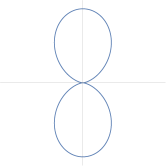
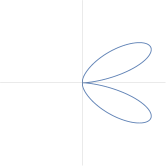
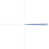
Figure 1: Rectilinear Angular Distribution; A polar plot with $\beta=0.0,0.33,$ $0.66,0.99$. The vertical axes is $x$ and the horizontal axis is $z$. The electron moves forward along the $z$ straight line direction.

Ultrator

Parator

Infrator

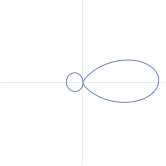
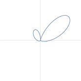
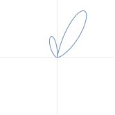
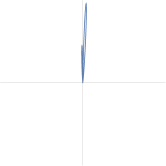
Figure 5: Catenary Angular Distribution; Additional torsion is added with substantial Rindler drift: $v_{R}=0.25$. Here $\beta=0.251,0.500,$ $0.749,0.998$ for the four plots respectively.

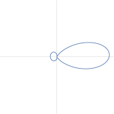
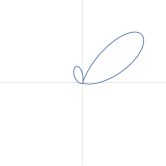
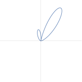
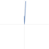
Figure 6: Catenary Angular Distribution; The Rindler drift requires an initial starting speed $\beta>v_{R}$. Here $v_{R}=0.333$, and $\beta=0.334$, $0.555$, $0.776$, $0.997$.

Chapter 14 Power Distributions 3D Plots

Nulltor

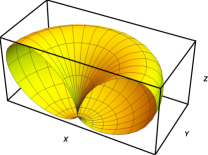
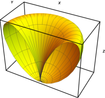
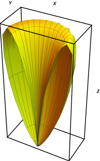
Figure 1: 3-Dimensional Angular Distribution; A polar plot with $\beta=0.3,$ $0.6,0.9$. The electron moves forward along the $+z$ direction. The plot range is $\theta=[0,\pi]$ and $\phi=[0,\pi]$.

Ultrator

Parator

Infrator

Hypertor

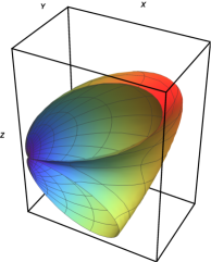
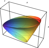
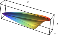
Figure 5: Helix Angular Distribution; $\kappa=1$, $\tau=\nu=0.1$, $\beta=0.3,0.6,$ $0.9$ . The plot range is $\theta=[0,\pi]$ and $\phi=[0,\pi]$.

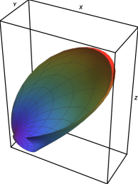
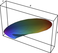
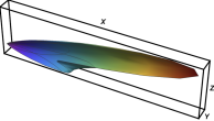
Figure 6: Hypertor Angular Distribution with invariants : $\kappa=1,\tau=\nu=0.5$, and speed $\beta=0.3,0.6,$ $0.9$ . The plot range is $\theta=[0,\pi]$ and $\phi=[0,\pi]$.