Orbital Deflection of Comets by Directed Energy

Abstract

Cometary impacts pose a long-term hazard to life on Earth. Impact mitigation techniques have been studied extensively, but they tend to focus on asteroid diversion. Typical asteroid interdiction schemes involve spacecraft physically intercepting the target, a task feasible only for targets identified decades in advance and in a narrow range of orbits—criteria unlikely to be satisfied by a threatening comet. Comets, however, are naturally perturbed from purely gravitational trajectories through solar heating of their surfaces which activates sublimation-driven jets. Artificial heating of a comet, such as by a laser, may supplement natural heating by the Sun to purposefully manipulate its path and thereby avoid an impact. Deflection effectiveness depends on the comet’s heating response, which varies dramatically depending on factors including nucleus size, orbit and dynamical history. These factors are incorporated into a numerical orbital model to assess the effectiveness and feasibility of using high-powered laser arrays in Earth orbit and on the ground for comet deflection. Simulation results suggest that a diffraction-limited 500 m orbital or terrestrial laser array operating at 10 GW for 1% of each day over 1 yr is sufficient to fully avert the impact of a typical 500 m diameter comet with primary nongravitational parameter $A_{1}=2\times 10^{-8}$ au d^-2. Strategies to avoid comet fragmentation during deflection are also discussed.

The Astronomical Journal, in press (accepted 2019 March 25)

1 Introduction

Earth-crossing asteroids and comets pose a long-term hazard to human interests on Earth. Numerous methods to mitigate the impact threat have been developed, but these generally focus on the asteroid threat while directing minimal attention toward cometary impactors. These methods include, but are not limited to:

1. Kinetic impactors, by which momentum is transferred to the asteroid via the hypervelocity impact of an expendable spacecraft, optionally enhanced by an explosive charge (McInnes, 2004; Koenig & Chyba, 2007).

2. Direct application of thrust, via thrusters placed directly onto the surface of the asteroid (Walker et al., 2005) or on one or more gravitationally-bound spacecraft positioned nearby as “gravity tractors” (Lu & Love, 2005; Foster et al., 2013).

3. Surface albedo alteration, such as by paint (Hyland et al., 2010) or mirrors (Vasile & Maddock, 2010) to slowly shift the asteroid’s orbit via radiation pressure.

These strategies all share one fundamental requirement: a spacecraft must physically intercept the target. This requirement is acceptable when the target follows a typical low-eccentricity, low-inclination orbit and is identified decades in advance of a potential impact, qualities shared by most near-Earth asteroids (NEAs).

These favorable qualities, however, are not common among comets, which are found at all inclinations and near-parabolic eccentricities. Long-period comets (LPCs), in particular, are rarely discovered more than 3 yr in advance of their closest approach to Earth (Francis, 2005). One recent example of an LPC, C/2013 A1 (Siding Spring), approached to within $140500$ km (0.37 LD) of Mars only 22 months after its discovery (Farnocchia et al., 2016). While further advancement in sky survey technology will somewhat improve the warning, discoveries of these comets remain fundamentally limited by their approach from the distant outer solar system, where they cannot be observed with telescopes of any realistic scale. Such short notice leaves little time to even design an interception mission, much less actually reach the comet in time to deflect it under a realistic delta-v budget. Any reliable method for diverting a comet from impact must be capable of operating remotely and commencing immediately following the identification of a threat.

One potentially viable approach for deflecting comets is directed energy heating, whereby a laser array concentrates energy onto the surface of the target, vaporizing it. The resulting ejecta plume exerts thrust on the object, shifting it from its original collisional trajectory (Lubin et al., 2014). One proposed option for deflecting NEAs is, in fact, to install the laser aboard a rendezvous spacecraft that intercepts and travels alongside the asteroid. Physical proximity of the laser, however, is not fundamentally required by the directed energy approach. The long-range nature of light implies that a laser array may also be built to operate from Earth orbit, or even from the ground, deflecting the target remotely. Such a system would permit an immediate response to any confirmed threat, including an LPC. Directed energy is particularly applicable as a method for comet deflection due to the volatile material—particularly water ice—on or near the surface of comets that drive their cometary activity. Nongravitational accelerations in response to solar heating have been astrometrically determined for numerous comets (Królikowska, 2004). The response of these comets to laser heating may then be estimated by scaling the measured solar heating accelerations under a standard heating model (Delsemme & Miller, 1971; Marsden et al., 1973).

The effectiveness of near-Earth object deflection via directed energy has been studied previously for several mission configurations, including the rendezvous case, in Zhang et al. (2016b). While cometary impactors are discussed, they are treated at a cursory level using a crude heating response model based on the one used for asteroids. The present manuscript serves as an extension to these earlier results and introduces new orbital simulations developed specifically to simulate comet deflection based on existing models of cometary nongravitational forces. In addition, complications specific to comet deflection, such the risk of fragmentation under heating, are also briefly addressed.

2 Simulations

The simulations model the Sun, the Moon, and the eight known major planets as Newtonian gravitational point sources in the frame of the solar system barycenter, with their positions given by JPL DE 421 (Folkner et al., 2008). The comet is treated as a test particle under the influence of the gravitational sources and of the laser, which is approximated as coincident with the center of the Earth at position $\bm{x}_{\oplus}$. Numerical integration is performed with the “s17odr8a” composition of the Velocity Verlet method (Kahan & Li, 1997).

Note that, while the Moon and planets other than Earth will significant alter the impact threat posed by a real comet, their inclusion in the presented simulations has a negligible effect on the results, as only comets following a direct impact trajectory are simulated. Prior close encounters with gravitational sources may amplify trajectory differences and thus improve deflection effectiveness. A random threatening LPC is unlikely to have had a close encounter with another planet before reaching Earth, so this scenario will not be further considered in this analysis.

2.1 Laser

Comet deflection is performed via heating of the target comet by a large array of phased laser elements. Laser pointing—performed by adjusting the phasing of the individual elements—is assumed to be perfect, with the laser beam exactly centered on the comet nucleus over the deflection period. Such accurate targeting may be achieved by scanning the laser beam and monitoring the reflection of the beam from the nucleus. The resulting astrometry of the nucleus will aid in constraining the trajectory of the comet both initially and over the course of the deflection process. This approach is similar to the one taken in Riley et al. (2014), which proposes to locate NEAs by monitoring return signals from a scanning laser beam.

Two classes of laser arrays are considered:

1. Orbital: the laser array is supported by a photovoltaic (PV) array operating in low-Earth orbit. Laser output is restricted by both an operating power $P$, constrained by the number of laser elements and by their heat dissipation mechanisms, and a time-averaged power $\langle P\rangle$, constrained by the size and efficiency of the PV array. In the simulations, the laser operates at $P$ when active; it is supported by the PV array directly, as well as by an attached battery system charged by the PV array when the laser is idle. Given a square PV array of edge length $L_{\text{PV}}$ and total solar-to-laser efficiency $\varepsilon$, average laser power is $\langle P\rangle=\varepsilon S_{0}L_{\text{PV}}^{2}$. The simulations consider the laser-carrying spacecraft to be equipped with a PV array of size $L_{\text{PV}}\sim L_{\text{las}}$, the size of the laser array itself. While not required in practice, this assumption is consistent with the orbital laser array designs discussed in Lubin et al. (2014) in which the PV and laser arrays together comprise the bulk of the spacecraft’s physical size.

2. Terrestrial: the laser array is installed directly on the Earth’s surface. Laser output is restricted to $P$, primarily due to the size of the array and the number of laser elements available. Electrical power and heat dissipation capacity impose lesser constraints. Mean power $\langle P\rangle=f(t)P$ varies over time $t$, where $f(t)$ is the average fraction of time each day the laser can target the comet. For the laser to be usable, the comet must be within the laser’s field of view of diameter $\Theta_{\text{fov}}$ centered on the zenith. This condition is dependent on the latitude of the laser $\phi_{\text{las}}$, as well as on the declination of the comet $\delta_{\text{com}}(t)$ as viewed from Earth. Operation is also constrained by $f(t)\propto\kappa$, the fraction of acceptable the weather expected at the site of the laser. Although $\kappa$ may vary on a seasonal basis depending on local climate, these variations are neglected for the simulations in which $\kappa$ is considered constant. Careful treatment of $\kappa$ is left to a more detailed study on laser site selection.

Both types of laser arrays are assumed to be capable of producing a diffraction-limited beam diverging at a half-angle $\theta_{\text{beam}}\approx\lambda_{\text{beam}}/L_{\text{las}}$ for a beam of wavelength $\lambda_{\text{beam}}\approx 1$ $\mu$m.

With a terrestrial array, an adaptive optics system to counteract atmospheric distortion is necessary to attain such a narrow beam. Such challenges faced in the construction and operation of these arrays have been—and are continuing to be—analyzed in detail separately, and will not be discussed in depth here (Lubin et al., 2014). Unless otherwise noted, the simulations assume these purely engineering challenges can and will be overcome.

2.2 Comet

The target comet is modeled as a non-rotating spherically-symmetric object with zero thermal inertia, using the semi-empirical nongravitational acceleration model of Marsden et al. (1973) based on the sublimation curve of water ice on the comet’s surface numerically computed by Delsemme & Miller (1971). Such a comet at barycentric position $\bm{x}$ illuminated by the Sun at $\bm{x}_{\odot}$, with $r\equiv\|\bm{x}-\bm{x}_{\odot}\|$, experiences a nongravitational acceleration, produced by jets powered by sublimating water ice, of

$$\ddot{\bm{x}}_{\text{NG}}=A\times\alpha\left(\frac{r}{r_{0}}\right)^{-m}\left(1+\left(\frac{r}{r_{0}}\right)^{n}\right)^{-k}\frac{\bm{x}-\bm{x}_{\odot}}{r}$$ (1)

with $r_{0}=2.808$ au, $\alpha=0.111262$, $m=2.15$, $n=5.093$, and $k=4.6142$. This notation is equivalent to $A_{1}=A$, $A_{2}=0$, $A_{3}=0$ in the original notation of Marsden et al. (1973), where $A_{2}$ and $A_{3}$ are analogous to $A$ for the components of $\ddot{\bm{x}}_{\text{NG}}$ orthogonal to $\bm{x}-\bm{x}_{\odot}$.

Nonzero comet nucleus rotation and thermal inertia will rotate $\ddot{\bm{x}}_{\text{NG}}$ away from the direction of $\bm{x}-\bm{x}_{\odot}$, producing non-radial components $A_{2}$, $A_{3}\neq 0$. With extremely fast rotation, $\ddot{\bm{x}}_{\text{NG}}$ weakens in magnitude as the heating thrust forces become spread over a wide range of directions. More detailed analyses of this effect are provided by Johansson et al. (2014) and Griswold et al. (2015), who discuss the heating response of small, rotating asteroids. Note that the structural and compositional inhomogeneity of comets complicates the exact results, although the underlying principles are similar. The considered $A_{2}=A_{3}=0$ of a non-rotating comet, however, serves as a good approximation for most comets, which feature $A_{1}\gg A_{2},A_{3}$ (Królikowska, 2004).

The nongravitational parameter $A$ (the acceleration at $r=1$ au) has been observationally measured for numerous comets and varies by several orders of magnitude between different comets depending on dynamical age, structure, and size (Yeomans et al., 2004). Assuming thrust $F_{\text{NG}}=m_{\text{com}}\ddot{x}_{\text{NG}}$ is proportional to the cross sectional area of sunlight intercepted by the comet, the nongravitational parameter is $A\propto R_{\text{com}}^{-1}\implies A\equiv A_{1\,\mathrm{km}}\left(1\,\mathrm{km}/2R_{\text{com}}\right)$ for comets of similar dynamical age and origin of diameter $2R_{\text{com}}$.

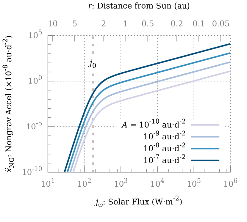
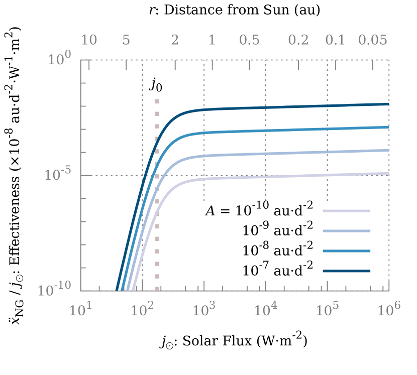
Figure 1: The nongravitational acceleration of a comet varies as a function of incident flux (left), and thus distance to the Sun, as given by Eqs. 1 and 2, based on the model developed by Marsden et al. (1973). A critical flux $j_{0}=172.6$ W m^-2 divides the response into a highly nonlinear ($j\ll j_{0}$) regime and a nearly linear ($j\gg j_{0}$) regime. Heating effectiveness (right), defined as the nongravitational acceleration per unit of incident flux, approximately follows a step function centered on $j_{0}$.

The simulations assume that energy absorption by the comet is wavelength-neutral, i.e., that the nucleus is neutrally colored and any dust coma surrounding the nucleus is optically thin. These conditions have thus far been met for all comets visited by spacecraft to date, with the latter condition likely met by all but a handful of comets with extremely low perihelia (Gundlach et al., 2012).

Under this assumption, the comet must necessarily respond equivalently to all incident optical radiation, regardless of origin, with the response depending only on the flux $j$ on the comet. By this “equivalence principle,” any radiation source at $\bm{x}_{0}$ (with $r^{\prime}\equiv\|\bm{x}-\bm{x}_{0}\|$) uniformly illuminating the cross section of the comet—including a laser with a beam that has sufficiently diverged to a cross section larger than the comet—will produce an acceleration

$$\ddot{\bm{x}}_{\text{NG}}=A\times\alpha\left(\frac{j}{j_{0}}\right)^{m/2}\left(1+\left(\frac{j}{j_{0}}\right)^{-n/2}\right)^{-k}\frac{\bm{x}-\bm{x}_{\odot}}{r^{\prime}}$$ (2)

where $j_{0}=172.6$ W m^-2 is the solar flux at $r=r_{0}$, given a solar irradiance of $S_{0}=1361$ W m^-2 at $r=1$ au (Kopp et al., 2005). The magnitude of single-source nongravitational acceleration is plotted in Fig. 1 in the context of the Sun. Two distinct regimes are evident:

1. Below a critical flux $j_{0}=172.6$ W m^-2, acceleration falls off rapidly as $\ddot{x}_{\text{NG}}\propto j^{12.83}$.

2. Above $j_{0}$, the function becomes nearly linear, approaching $\ddot{x}_{\text{NG}}\propto j^{1.075}$.

The effectiveness of the heating—the amount of nongravitational acceleration per unit of incident flux—is evidently closely approximated by a step function separating the two regimes. Thus, each unit of flux only contributes significantly to accelerating the comet with total incident flux in the latter regime.

Eq. 2, however, only gives the acceleration from a single radiation source. It is valid, for example, when the comet is only being illuminated by the Sun, or is only being illuminated by the laser. In a comet deflection scenario, both sources generally must be considered. Because Eq. 2 as a whole is highly nonlinear, the acceleration from the superposition of the two sources is nontrivial and requires additional assumptions regarding the actual distribution of thrust over the comet’s surface.

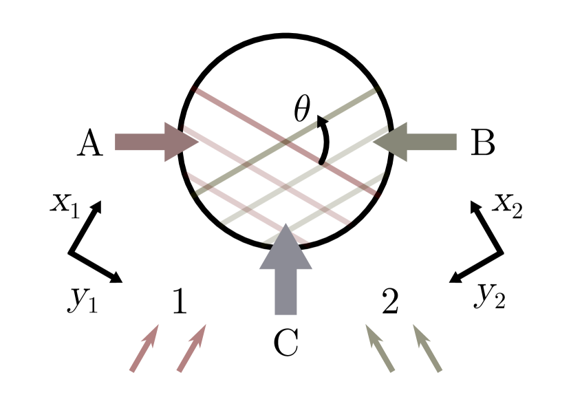
Figure 2: A comet being deflected is, in general, illuminated from two different directions by two different radiation sources (the Sun and the laser). In this diagram, source 1 illuminates the lower left (red stripes) of the comet (circle) and source 2 illuminates the lower right (green stripes), with the sources separated by an angle $\theta$. The illuminated fraction of the comet is divided into three regions: region A is illuminated by source 1 alone, region B is illuminated by source 2 alone, and region C is illuminated by both. Arrows directed into the comet indicate the assumed direction of acceleration contributed by each region—the mean inward normal direction of the region—used in the simulations.

Consider two radiation sources 1 and 2, representing the Sun and the laser, illuminating the comet and separated by angle $\theta$ as illustrated in Fig. 2. The illuminated fraction of the comet is divided into three regions:

1. Region A, illuminated by source 1 alone.

2. Region B, illuminated by source 2 alone.

3. Region C, illuminated by both.

Due to the curvature of the comet’s surface, the surface itself is not uniformly illuminated in any of the three regions, despite the cross section being uniformly illuminated. Precise determination of the acceleration contributed by each region requires a detailed thermal model for the surface response to incident radiation. Results from such a model, which assumes a spherical comet, still only provide a rough approximation for the acceleration of a realistic comet. Comparable accuracy to a realistic comet may be attained by simply considering the acceleration contributed by each region to be in the mean inward normal direction of the region, as indicated in Fig. 2.

We first select $\hat{\bm{x}}_{1}$ to be the propagation direction of radiation from source 1, and $\hat{\bm{y}}_{1}$ a perpendicular direction in the plane of both sources and the comet, as indicated in Fig. 2. When source 2 is inactive (i.e., no laser), the two-source model—the sum of the accelerations contributed by region A and region C—must be consistent with the single source model. Let $\ddot{\bm{x}}_{A}$ be the acceleration contributed by region A and $\ddot{\bm{x}}_{C}$ be the acceleration by region C. The sum $\ddot{\bm{x}}_{1}\equiv\ddot{\bm{x}}_{A}+\ddot{\bm{x}}_{C}$ must match the expression for $\ddot{\bm{x}}_{\text{NG}}$ given in Eq. 2. Matching the components in $\hat{\bm{x}}_{1}$ and $\hat{\bm{y}}_{1}$ gives

$$\begin{cases}\ddot{x}_{1}&=\ddot{x}_{A}\sin(\theta/2)+\ddot{x}_{C}\cos(\theta/2)\\ 0&=\ddot{x}_{A}\cos(\theta/2)-\ddot{x}_{C}\sin(\theta/2)\end{cases}$$ (3)

so $\ddot{x}_{A}=\ddot{x}_{1}\sin(\theta/2)$ and $\ddot{x}_{C}=\ddot{x}_{1}\cos(\theta/2)$ are the magnitudes of the acceleration contributions of the two regions.

When source 2 is activated, region A experiences no change, so $\ddot{x}_{A}$ remains unaffected. By symmetry, region B contributes an acceleration of $\ddot{x}_{B}=\ddot{x}_{2}\sin(\theta/2)$, where $\ddot{\bm{x}}_{2}$ is the acceleration given by Eq. 2 for source 2 alone. Finally, the acceleration contributed by region C becomes roughly $\ddot{x}_{C}=\ddot{x}_{1+2}\cos(\theta/2)$, where $\ddot{\bm{x}}_{1+2}$ is the acceleration by Eq. 2 for a single source with the combined flux of both source 1 and source 2. The net nongravitational acceleration on the comet is then the vector sum

$$\ddot{\bm{x}}_{\text{NG}}=\ddot{\bm{x}}_{A}+\ddot{\bm{x}}_{B}+\ddot{\bm{x}}_{C}$$ (4)

This two-source model degenerates into special cases of the one-source model as expected in both the $\theta\to 0$ limit (i.e., comet at distance $r\gg 1$ au, the separation of the Sun and the Earth/laser), where $\ddot{\bm{x}}_{\text{NG}}\to\ddot{\bm{x}}_{1+2}$, and in the $\theta\to\pi$ limit (i.e., comet directly between Sun and laser) where $\ddot{\bm{x}}_{\text{NG}}\to\ddot{\bm{x}}_{1}+\ddot{\bm{x}}_{2}$, a simple superposition of the one-source accelerations.

In the simulations, source 1 is the Sun, with an incident flux $j_{1}=S_{0}\times(\text{1 au}/r)^{2}$. Source 2 is the laser, at distance $\Delta\equiv\|\bm{x}-\bm{x}_{\oplus}\|$ from the comet, producing a spot of radius $R_{\text{spot}}=\theta_{\text{beam}}\Delta$ with flux $j_{2}=P_{\text{peak}}/\left(\pi R_{\text{spot}}^{2}\right)$ when active.

The two-source model above is only valid when $R_{\text{spot}}>R_{\text{com}}$, i.e., when the cross section of the comet is uniformly illuminated. In the limit $j_{2}\gg j_{1}$ and $R_{\text{spot}}\ll R_{\text{com}}$ (but with $R_{\text{spot}}$ still sufficiently large to neglect thermal diffusion across the surface—a condition assumed to always hold), the laser-contributed acceleration decouples from the solar acceleration $\ddot{\bm{x}}_{\odot}$ in Eq. 1 to give

$$\ddot{\bm{x}}_{\text{s}\ll\text{c}}=\ddot{\bm{x}}_{\odot}+\left(R_{\text{spot}}/R_{\text{com}}\right)^{2}\ddot{\bm{x}}_{2}$$ (5)

where $\ddot{\bm{x}}_{2}$ is the one-source acceleration by a laser of the same flux $j_{2}$ illuminating the entire comet cross section.

Note that the scaling relation in Eq. 5 assumes that the rotation-averaged heating response of the comet is uniform at the scale of the laser spot. Small-scale variations in terrain may cause the net thrust to be directed in an unexpected direction, challenging the earlier assumption of a dominant radial component of nongravitational acceleration. This problem can be corrected by dithering the position of the laser spot on the comet, which will average over these variations.

For intermediate $R_{\text{spot}}<R_{\text{com}}$ but $R_{\text{spot}}\not\ll R_{\text{com}}$, linear interpolation (in area) between the $R_{\text{spot}}\to 0$ limit and the case $R_{\text{spot}}\to R_{\text{com}}$ with $j_{2}\to j_{2}^{\prime}=j_{2}\left(R_{\text{spot}}/R_{\text{com}}\right)^{2}$ is used. Total nongravitational acceleration by the Sun and laser is therefore

$$\ddot{\bm{x}}_{\text{$\odot$,las}}=\begin{cases}\left(1-\left(R_{\text{spot}}/R_{\text{com}}\right)^{2}\right)\ddot{\bm{x}}_{\text{s}\ll\text{c}}\\ \>+\left(R_{\text{spot}}/R_{\text{com}}\right)^{2}\ddot{\bm{x}}_{\text{NG}}(j_{1},j_{2}^{\prime}),&R_{\text{spot}}<R_{\text{com}}\\ \ddot{\bm{x}}_{\text{NG}}(j_{1},j_{2}),&R_{\text{spot}}\geq R_{\text{com}}\end{cases}$$ (6)

When $\langle P\rangle<P$, the laser is idle for a fraction of time and $\ddot{\bm{x}}_{\text{NG}}$ becomes an appropriate linear combination of $\ddot{\bm{x}}_{\text{$\odot\ $only}}$ from Eq. 1 with the Sun alone, and $\ddot{\bm{x}}_{\text{$\odot$,las}}$ from Eq. 6 with the Sun and laser together:

$$\ddot{\bm{x}}_{\text{NG}}=\left(1-\langle P\rangle/P\right)\ddot{\bm{x}}_{\text{$\odot\ $only}}+\left(\langle P\rangle/P\right)\ddot{\bm{x}}_{\text{$\odot$,las}}$$ (7)

Finally, there may be times when it is not advantageous to keep the laser active, even when line of sight and power restrictions permit, as perturbations to the orbit from laser heating at one part of the orbit may cancel perturbations from laser heating at a different part of the orbit (Zhang et al., 2016b). Perturbation cancellation may be minimized by tracking the sign of $\xi\equiv(\bm{x}_{\text{com}}-\bm{x}_{\oplus})\cdot\dot{\bm{x}}_{\text{com}}$ and permitting the laser to activate either only when $\xi>0$ (laser is “behind”) or only when $\xi<0$ (laser is “ahead”). The simulations focus primarily on deflecting comets with long orbital periods $\gtrsim$100 yr, where deflection occurs only over the final fraction of an orbit before its Earth encounter. Thus, $\xi<0$ nearly always holds, and so the laser “ahead” condition is chosen.

2.3 Numerical Setup

The original orbit of the comet is specified by its perihelion distance $q$, inclination $i$, eccentricity $e$, time of impact $T$, whether impact occurs at the ascending or descending node, and whether impact occurs before or after perihelion.

Next, initial conditions for the comet are found by the following procedure:

1. Choose $\bm{x}_{0}(T)=\bm{x}_{\oplus}(T)$ as the final position of the comet in its natural orbit.

2. Compute $\dot{\bm{x}}_{0}(T)$ such that the heliocentric Keplerian orbit fit through $\bm{x}_{0}(T)$, $\dot{\bm{x}}_{0}(T)$ matches the specified orbital parameters.

3. Using the Keplerian orbit of the comet, find the smallest $\delta t>0$ such that $\|\bm{x}_{0}(T-\delta t)-\bm{x}_{\oplus}(T-\delta t)\|=R_{\oplus}$, the radius of the Earth.

4. Increase $\dot{x}_{0}(T-\delta t)\to\dot{x}_{0}(T-\delta t)+\sqrt{2GM_{\oplus}/R_{\oplus}}$ to account for Earth’s gravitational well, where $M_{\oplus}$ is the mass of the Earth.

5. Numerically integrate time-reversed system in the solar system potential with $\ddot{\bm{x}}_{\text{NG}}$ from Eq. 1 to find $\bm{x}(t_{0})$, $\bm{\dot{x}}(t_{0})$, the state vector at time $t=t_{0}$ when the laser is to be first activated.

Using $\bm{x}(t_{0})$, $\bm{\dot{x}}(t_{0})$ as initial conditions, numerical integration proceeds using the same solar system potential, with $\ddot{\bm{x}}_{\text{NG}}$ from Eq. 7. The system is integrated either to $t=T$ (yielding $\bm{x}(T)$, $\bm{\dot{x}}(T)$) or until $\Delta(t)\equiv\|\bm{x}(t)-\bm{x}_{\oplus}(t)\|<R_{\oplus}$ where the comet impacts the Earth.

3 Results

For each comet deflection scenario, a deflection distance $\Delta_{\text{def}}$ quantifies the effectiveness of the deflection. For comets with a local minimum $\Delta_{\text{min}}=\Delta(t_{\text{min}})>R_{\oplus}$ (no impact), use $\Delta_{\text{def}}=\Delta_{\text{min}}$. Otherwise, define the true time of impact $t_{\text{imp}}$ as $\Delta(t_{\text{imp}})=R_{\oplus}$ and $\dot{\Delta}(t_{\text{imp}})<0$. Deflection distance $\Delta_{\text{def}}$ is then defined as the corresponding $\Delta_{\text{min}}$ for the trajectory $\bm{x}_{1}(t)$ with $\bm{x}_{1}(t_{\text{imp}})=\bm{x}(t_{\text{imp}})$ and $\dot{\bm{x}}_{1}(t)=\dot{\bm{x}}(t_{\text{imp}})$, the linear continuation of the comet’s trajectory through the Earth.

A typical comet discovered in the near future might follow a timeline similar to that of the recent dynamically new comet C/2013 A1 (Siding Spring), which passed Mars at a distance of 140500 km (0.37 LD) in 2014 October, just 22 months after discovery (Farnocchia et al., 2016). Continuing advancements in survey capability may conceivably extend the advance notice by a few months to years in the near future, though detection of such comets is ultimately limited by their trajectories, approaching from the distant outer solar system.

A future Earth-bound comet might be discovered $\sim$3 yr in advance, permitting impact confirmation and laser activation by 2 yr prior to the Earth encounter. For the simulations, consider a similar $2R_{\text{com}}=\,\mathrm{500}$ m diameter comet with $A=2\times 10^{-8}$ au d^-2 ($A_{1\,\mathrm{km}}=1\times 10^{-8}$ au d^-2) in a comparable orbit of $q=0.9$ au, $e=1$, $i=130\degree$ leading to an Earth impact at $T=\text{J2000.0}$ at its ascending node while the comet is inbound. These parameters for this canonical comet are used for all simulations, except when otherwise noted.

Note that the assumed value of $A_{1\,\mathrm{km}}=1\times 10^{-8}$ au d^-2 is lower than that of typical LPCs with $A_{1\,\mathrm{km}}\sim 10^{-7}$ au d^-2 or even $A_{1\,\mathrm{km}}\sim 10^{-6}$ au d^-2 (Królikowska, 2004). Simulation results will therefore underestimate deflection distance for these more responsive comets by a corresponding factor of 1–2 orders of magnitude. Meanwhile, periodic comets (JFCs and HTCs) vary in their composition, due to variation in dynamical age, and may have comparable $A_{1\,\mathrm{km}}\sim 10^{-8}$ au d^-2 or lower, with nongravitational deflection often not detectable at all if volatiles are sufficiently depleted. The presented results focus on the case of LPC impactors, which are associated with the extremely short warning times and cannot be reliably be deflected by any other proposed method. For these cases, the canonical comet described above provides an adequate, conservative example.

3.1 Orbital Laser

A laser array in Earth orbit is restricted in $\langle P\rangle$ by the size and efficiency of its PV array. Consider a square PV array with edge length $L_{\text{las}}$, equal in size to the laser array. For a total solar-to-laser power efficiency $\varepsilon=20\%$, such a system produces $\langle P\rangle=\varepsilon S_{0}L_{\text{las}}^{2}$. With $\varepsilon$ constrained by technology and thermodynamics, $\langle P\rangle$ can only reliably be improved by scaling up the array. Use of a supplementary battery system, however, allows $P\gg\langle P\rangle$.

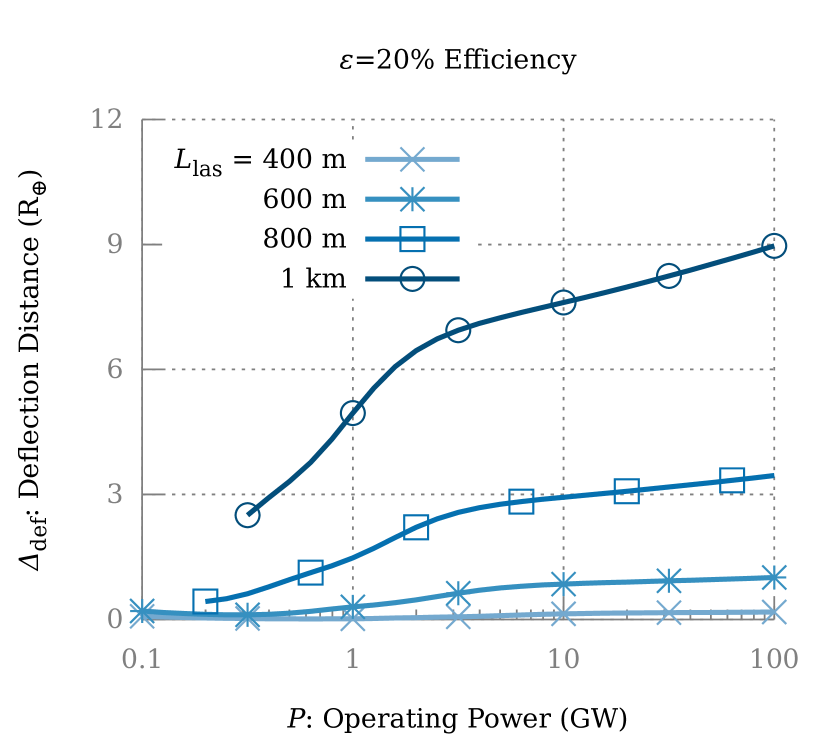
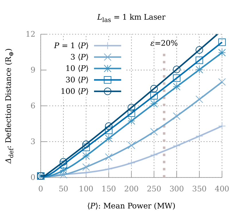
Figure 3: Deflection of the canonical comet by orbital laser arrays over 2 yr: Increasing $P$, even with a fixed $\langle P\rangle$, yields a substantial improvement in deflection due to the nonlinear heating response of the comet illustrated in Fig. 1. Note that $P\geq\langle P\rangle$, so curves are terminated at the lower end $P=\langle P\rangle$ (left) by this condition.

Fig. 3 illustrates the effectiveness of arrays with a range of $L_{\text{las}}$, $\langle P\rangle$ and $P$ for deflecting the canonical comet over 2 yr. Increasing array size $L_{\text{las}}$ and efficiency $\varepsilon$ both yield a substantial improvement in deflection distance $\Delta_{\text{def}}$. Furthermore, an increase in $P$ alone leads to a significant increase in $\Delta_{\text{def}}$. This result illustrates the nonlinear behavior of Eq. 1, which makes each unit of incident flux much more effective at accelerating the comet at $j\gg j_{0}$ than at $j\ll j_{0}$, as shown in Fig. 1. Increasing $P$ extends the range over which the comet can be illuminated at $j\gg j_{0}$, enabling a greater deflection distance for the same amount of energy. Note, however, that when $P$ is sufficiently high, the comet will be illuminated at $j\gg j_{0}$ for the entirety of the deflection, and further increases in $P$ will have little effect on heating effectiveness, and thus, $\Delta_{\text{def}}$.

It is conceivable that comet detection capability advances sufficiently by the time a threatening comet is identified that deflection may begin as early as $t_{0}=T-5$ yr for larger comets, which may permit the use of a smaller laser array. However, at such an early time, the comet is a large distance $r\text{, }\Delta\sim 15$ au from both the Sun and the laser. Without a sufficiently high operating power, the flux on the comet will fall deep within the $j\ll j_{0}$ regime and little deflection will occur until the comet approaches to a much closer distance.

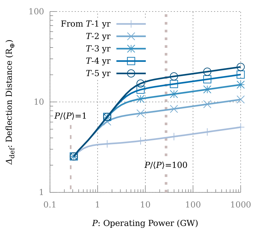
Figure 4: Effectiveness of a $L_{\text{las}}=1$ km laser with $\varepsilon=20\%$ operating at various $P$: Starting deflection earlier is only of measurable benefit if $P$ is sufficient high for $j\gg j_{0}$ on the comet to give non-negligible acceleration at the beginning of the deflection period.

Fig. 4 compares the effectiveness of several deflection start times for a smaller $L_{\text{las}}=500$ m laser with $\varepsilon=20\%$ efficiency. Operating at $P=100\langle P\rangle=7$ GW, the canonical comet is deflected $\Delta_{\text{def}}\sim 20$ $R_{\oplus}$ when deflection begins at $T-2$ yr. Beginning deflection even earlier achieves little additional gain in deflection, in the absence of an additional increase in $P$.

This effect is further illustrated by Fig. 5, which shows the accumulation of deflection of a set of canonical comets by laser arrays of various sizes operating at $P/\langle P\rangle=100$ and $\varepsilon=20\%$, beginning at $t=T-5$ yr. Over the first 3 yr, a $L_{\text{las}}=400$ m laser is incapable of deflecting the comet by even 0.1 $R_{\oplus}$, as $j\ll j_{0}$ over this period. The bulk of the eventual $\Delta_{\text{def}}=3.5$ $R_{\oplus}$ is accumulated over the final 1 yr. In contrast, the higher flux attained by laser arrays of $L_{\text{las}}\gtrsim 600$ m begins to accumulate deflection immediately at $t=t_{0}=T-5$ yr. Note that the final months of deflection contribute negatively to the final $\Delta_{\text{def}}$. Optimal deflection requires terminating the deflection process a few months before the comet arrives at Earth. As the loss in the final $\Delta_{\text{def}}$ is generally under 1 $R_{\oplus}$, no attempt is made to precisely determine the optimal cutoff time for these results, as this effect is dwarfed by the uncertainties associated with comet deflection discussed earlier.

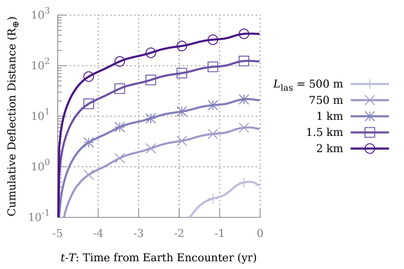
Figure 5: Deflection of the canonical $2R_{\text{com}}=500$ m comet is illustrated for laser arrays of various sizes operating at $P/\langle P\rangle=100$ and $\varepsilon=20\%$ beginning at $t_{0}=T-5$ yr. This plot shows the cumulative deflection distance at time $t$—the deflection distance $\Delta_{\text{def}}$ if the deflection process were to terminate at time $t$—over the interval of deflection. Note that deflection in the final months opposes the deflection accumulated earlier, so maximal deflection is actually attained a few months before the comet arrives at Earth.

Note that a laser at $P/\langle P\rangle=100$ would operate for an average of only 14.4 min each day, during which time the energy collected over an entire day is drained. Achieving such high $P/\langle P\rangle$, which requires a high-density laser array, while maintaining $\varepsilon$ may not necessarily be less of an engineering challenge than constructing a larger and equally effective array at lower $P/\langle P\rangle$. Analysis of optimal $P/\langle P\rangle$ is left to a more thorough investigation of orbital laser array construction. The remainder of this section considers arrays operating at $P/\langle P\rangle=100$.

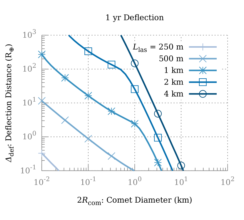
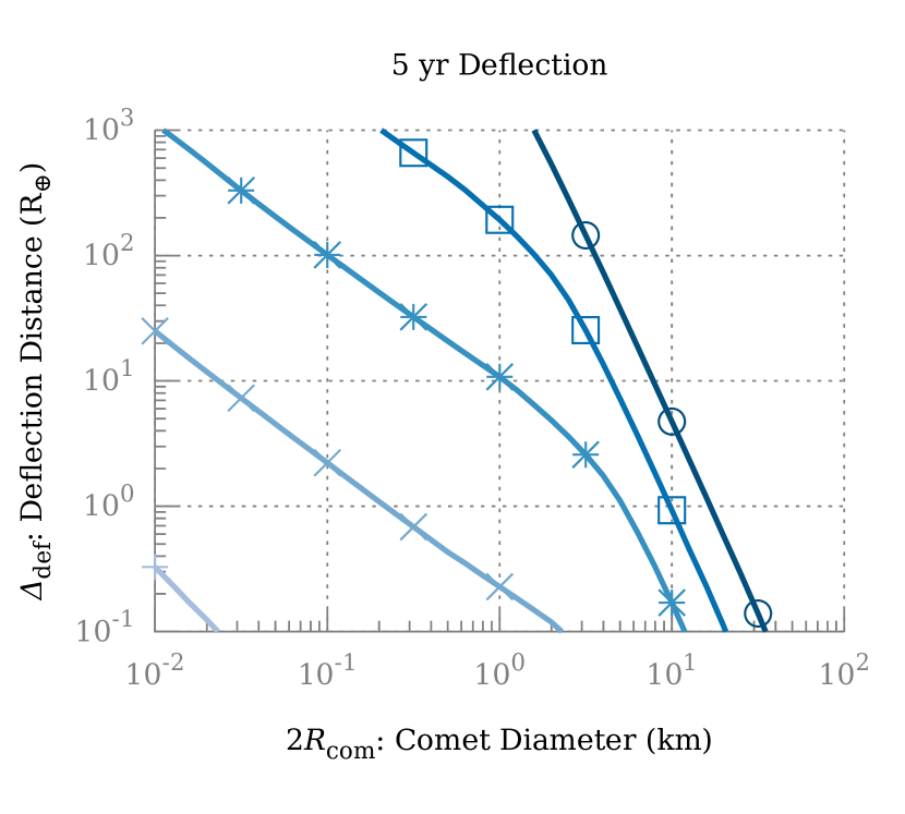
Figure 6: Under a fixed $A_{1\,\mathrm{km}}=1\times 10^{-8}$ au d^-2, deflection distance $\Delta_{\text{def}}$ scales roughly as $\Delta_{\text{def}}\propto R_{\text{com}}^{-1}$ at small $R_{\text{com}}$, for which $R_{\text{spot}}>R_{\text{com}}$ during most of the deflection period, and as $\Delta_{\text{def}}\propto R_{\text{com}}^{-3}$ at large $R_{\text{com}}$, for which $R_{\text{spot}}<R_{\text{com}}$ during most of the deflection period. In addition, larger laser arrays, which are needed to deflect larger comets, benefit more from longer deflection periods. With 1 yr available for deflection (left), a $L_{\text{las}}=1$ km laser can deflect a $2R_{\text{com}}=1$ km comet by $\Delta_{\text{def}}\approx 2$ $R_{\oplus}$. Given 5 yr (right), the same laser can deflect a larger 3 km comet by the same distance. Note that $\Delta_{\text{def}}\propto A_{1\,\mathrm{km}}$, so for highly active LPCs with $A_{1\,\mathrm{km}}\sim 10^{-7}$–$10^{-6}$ au d^-2, these curves would shift upward by a corresponding 10–$100\times$.

A larger array or additional warning time is necessary to divert comets of $2R_{\text{com}}>1$ km. Fig. 6 shows that $\Delta_{\text{def}}\propto R_{\text{com}}^{-3}$ for a given $A_{\text{$1\,\mathrm{km}$}}$. With 1 yr available for deflection, a $L_{\text{las}}=1$ km laser can deflect a $2R_{\text{com}}=1$ km comet by $\Delta_{\text{def}}=3$ $R_{\oplus}$. Given 5 yr, the same laser can deflect a much larger $2R_{\text{com}}=3$ km comet by the same distance. Very large comets of $2R_{\text{com}}>10$ km require very large laser arrays of $L_{\text{las}}\gtrsim 4$ km with $\gtrsim$5 yr to safely deflect. It is important to remember that all of the simulations assume the canonical $A_{1\,\mathrm{km}}=1\times 10^{-8}$ au d^-2. Because $\Delta_{\text{def}}\propto A_{1\,\mathrm{km}}$, if these comets behave similarly to volatile-rich LPCs with $A_{1\,\mathrm{km}}\sim 10^{-7}$–$10^{-6}$ au d^-2, deflection becomes a corresponding 10–$100\times$ more effective, and a $L_{\text{las}}=1$ km laser may be enough to deflect such a 5–10 km comet in 1 yr or a 10–20 km comet in 5 yr.

Deflection effectiveness drops rapidly with decreasing array size. At $P/\langle P\rangle=100$, $L_{\text{las}}=500$ m appears to be the smallest useful array for comet deflection, and is capable of deflecting a canonical $2R_{\text{com}}=50$ m comet by $\Delta_{\text{def}}=10$ $R_{\oplus}$. Note that, because the simulations assume $A$ and $R_{\text{com}}$ remain static throughout the deflection, results for small comets, which are more strongly altered by the deflection process, should be treated with caution.

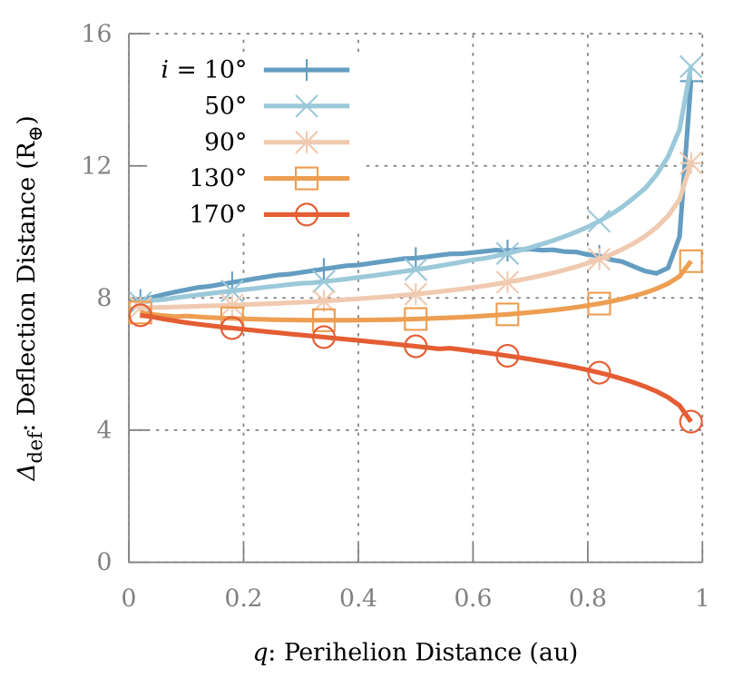
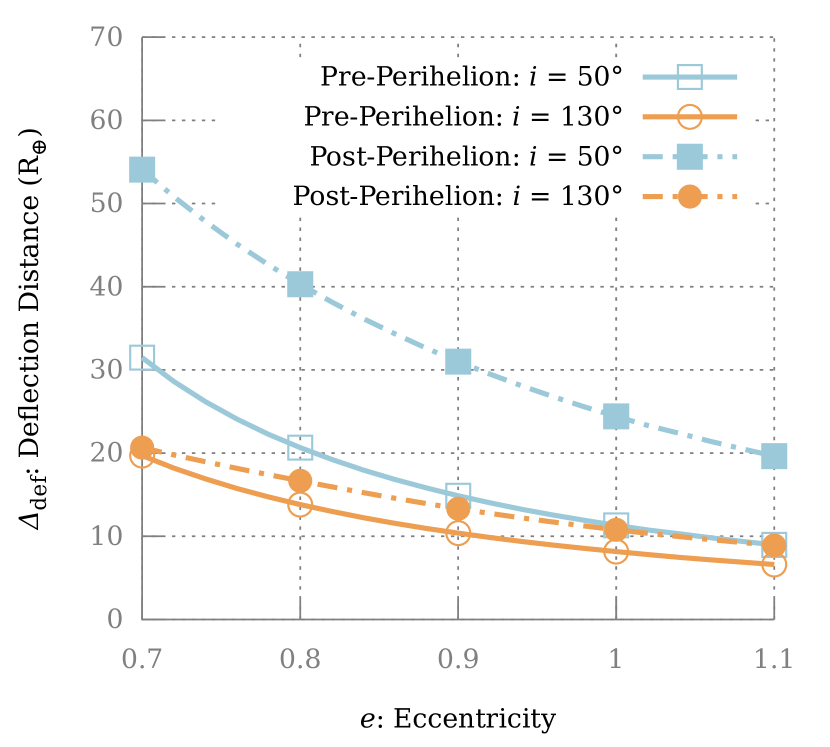
Figure 7: Deflection effectiveness of a $L_{\text{las}}=1$ km, $P=100\langle P\rangle$ orbital laser targeting copies of the canonical comet with modified orbital elements over 2 yr. High-inclination prograde orbits are most favorable to deflection, while low-inclination retrograde orbits are least favorable (left). Furthermore, a pre-perihelion impact appears to be more difficult to mitigate than a post-perihelion impact, particularly for comets in prograde orbits (right).

Finally, because the solar system is not gravitationally isotropic about the Earth, the deflection effectiveness of a given laser system varies depending on the exact orbit of the comet. Generally, deflection is most effective for orbits that place the comet near the laser for long durations over the deflection period, because $\ddot{x}_{\text{NG}}$ is an increasing function of $j\propto\Delta^{-2}$.

Fig. 7 shows the variations in effectiveness for a $L_{\text{las}}=1$ km, $P=100\langle P\rangle$ laser deflecting an otherwise canonical comet, beginning at $T-1$ yr over a range of plausible orbital parameters. For this case, high-inclination prograde orbits are most favorable and low-inclination retrograde orbits are least favorable, from a deflection standpoint. Furthermore, an impact while the comet is inbound is more difficult to mitigate than if the impact occurred were while the comet is outbound. The latter phenomenon is explained by the comet’s final approach to Earth: a comet approaching from within the Earth’s orbit (post-perihelion encounter) approaches more rapidly and spends less time near the Earth than an otherwise identical comet approaching from beyond Earth’s orbit (pre-perihelion encounter). In all cases, the variation in effectiveness from orbital differences is within a factor of 2—no more than the variation in $A_{1\,\mathrm{km}}$ between dynamically similar comets (Yeomans et al., 2004).

Lasers with larger $L_{\text{las}}$ starting at earlier $t_{0}$ experience increasingly less variation between comets of different orbits as deflection occurs over a spatial scale much larger than Earth’s orbit with $j>j_{0}$ over a much longer distance. At such scale, the gravitational potential of the solar system is nearly isotropic about the laser (which, at large scale, is located near the center of the solar system) and deflection approaches the orbit-neutral limit. Conversely, small lasers are affected more strongly by the orbit of the comet, an effect that becomes important for ground-based lasers which may be useful for deflection at much smaller scales.

3.2 Terrestrial Laser

Unlike the case for orbital arrays, $\langle P\rangle$ is not restricted by $L_{\text{las}}$ for terrestrial laser arrays where electric power may be supplied externally. For a given $P$, $\langle P\rangle$ is only restricted by the requirement that the comet be within the laser’s field of view $\Theta_{\text{fov}}$ and that weather conditions permit operation. Achieving the necessary diffraction-limited beam from the ground poses a serious challenge for very large $L_{\text{las}}$ with their tiny $\theta_{\text{beam}}$. These constraints favor compact but high-powered arrays.

Terrestrial lasers are directionally biased by the nature of their fixed field of view relative to Earth. A laser at latitude $\phi_{\text{las}}$ with field of view $\Theta_{\text{fov}}$ may only target comets in declinations $\phi_{\text{las}}-\Theta_{\text{fov}}/2<\delta_{\text{com}}<\phi_{\text{las}}+\Theta_{\text{fov}}/2$. A laser at a far northern latitude is completely ineffective against a comet approaching from near the southern celestial pole, as such a comet never rises sufficiently high in the sky to enter the laser’s field of view.

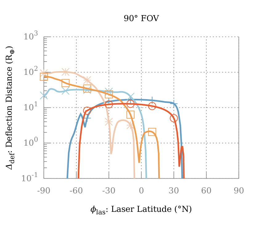
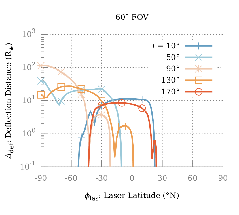
Figure 8: Deflection effectiveness of $L_{\text{las}}=500$ m, $P=25$ GW terrestrial lasers located at various latitudes $\phi_{\text{las}}$ with identical $\kappa=50\%$ targeting copies of the canonical comet of various inclinations $i$ over 2 yr: A laser with a $90\degree$ field of view (left) is more effective against a wider range of comets, than an otherwise identical laser with a $60\degree$ field of view (right).

Fig. 8 compares the deflection effectiveness against a set of modified canonical comets of various $i$ by a $L_{\text{las}}=500$ m, $P=25$ GW array at $\kappa=50\%$ for $\Theta_{\text{fov}}=90\degree$ and $\Theta_{\text{fov}}=60\degree$. The laser with the larger $90\degree$ field of view targets the comet longer than a laser with the smaller $60\degree$ field of view, and thus it produces a larger deflection $\Delta_{\text{def}}$ and is effective over a wider range of latitudes $\phi_{\text{las}}$.

Prograde orbits ($i<90\degree$) are strongly favored over retrograde ($i>90\degree$), due to prograde-orbiting comets having slower relative velocity in the final approach. The variations for the $L_{\text{las}}=500$ m terrestrial laser are far more significant than those of the $L_{\text{las}}=1$ km orbital laser, due to the spatial scale differences discussed in the previous section. Note that these results are for an Earth encounter at the comet’s ascending node where the comet approaches from below the ecliptic, favoring deflection from the southern hemisphere. Descending node encounters correspond to similar results, but mirrored to favor deflection from the northern hemisphere. Zhang et al. (2017) explore the directional biases of terrestrial lasers in more detail, in the context of historical cometary orbits.

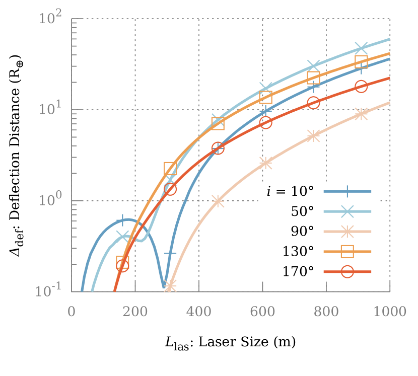
Figure 9: Deflection effectiveness of $P=1$ GW terrestrial laser arrays of a range of sizes located at $\phi_{\text{las}}=30\degree\text{S}$ with $\Theta_{\text{fov}}=90\degree$ for comets of various inclinations $i$ over 2 yr: At $L_{\text{las}}\lesssim 200$ m, beam divergence prevents significant deflection until a few months prior to encounter, a period where deflection opposes earlier deflection as shown in Fig. 5, resulting in the interval of negative slope near $L_{\text{las}}\sim 200$ m for the prograde comets.

Increasing $L_{\text{las}}$, which provides a tighter beam, will also improve deflection, even without a corresponding increase in $P$. Fig. 9 compares the deflection effectiveness by $P=1$ GW arrays over a range of $L_{\text{las}}$. Increasing from $L_{\text{las}}=500$ m to $L_{\text{las}}=1$ km boosts the deflection to a very safe $\Delta_{\text{def}}=10$–30 $R_{\oplus}$, depending on the comet’s orbit.

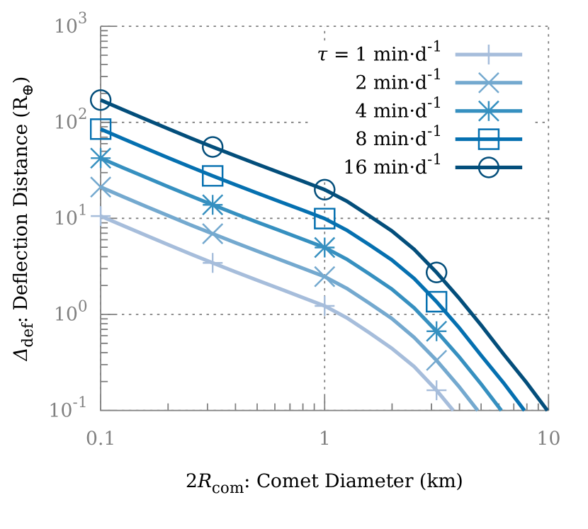
Figure 10: A single $L_{\text{las}}=1$ km operating at $P=100$ GW for a few minutes each day over 2 yr is sufficient to deflect many comets. At $\tau=4$ min d^-1, such a system can deflect the canonical $2R_{\text{com}}=500$ m comet by a comfortable $\Delta_{\text{def}}\sim 10$ $R_{\oplus}$. Targeting of the comet is assumed to be possible for $\geq\tau$ throughout the deflection period.

Extremely large and powerful ground-based laser arrays of $L_{\text{las}}=1$ km and $P=100$ GW have been proposed to enable near-relativistic spaceflight by radiation pressure on thin, reflective sails (Lubin, 2016; Kulkarni et al., 2018). Such laser arrays, however, may only operate for a short fraction $\tau\ll 1$ of each day ($P/\langle P\rangle=\tau^{-1}\gg 1$). Fig. 10 compares deflection for $\tau=1$ min d^-1 to 16 min d^-1. An array at $\tau=2$ min d${}^{-1}=1/720$, installed at an appropriate site, can safely deflect a canonical $2R_{\text{com}}=500$ m comet by a comfortable $\Delta_{\text{def}}\sim 10$ $R_{\oplus}$ over 1 yr. With $\tau=16$ min d${}^{-1}=1/90$, the same laser can deflect a $2R_{\text{com}}=1$ km by approximately the same distance.

Ultimately, regardless of its power, size and location, a single terrestrial laser array is insufficient as a long-term solution for comet deflection, due its limited field of view. A robust terrestrial planetary defense system will require multiple laser arrays distributed across a wide enough range of latitudes to provide full sky coverage. With such a network, every point on the celestial sphere is in the field of view of at least one laser at some point each day, ensuring the ability to target comets approaching in any orbit.

3.3 Fragmentation Mitigation

Active comets—especially dynamically new comets entering the inner solar system for the first time—have a propensity to disintegrate under solar heating (Boehnhardt, 2004). Laser heating of the nucleus supplements the natural solar heating, elevating the likelihood of fragmentation. When presented with a threatening comet with insufficient notice to carry out a successful deflection, laser-induced fragmentation could be used, if the consequence of impact by an intact nucleus is determined to be more severe than impact by multiple small fragments. Fragmentation, however, hinders a clean deflection—the focus of these simulations—converting a single nucleus into several smaller nuclei that must be deflected simultaneously, which may not be possible.

Beyond a few specific instances, the process of comet splitting is not well understood. Circumstances for disintegration vary dramatically between comets, with some surviving until within a few radii of the Sun, and others fragmenting well beyond the orbit of the Earth (Boehnhardt, 2004). The mechanisms proposed for fragmentation under illumination generally reflect the following pattern:

1. Cumulative loss of volatiles from the nucleus, weakening its structure;

2. Stress from sublimation pressure overcoming the remaining strength of the nucleus.

These simulations treat the comet as time-independent, with fixed $A$ throughout the entire deflection process. This assumption is valid when volatile loss during deflection—comparable to, at most, the volatile loss expected during one perihelion passage for the scenarios considered—is negligible compared to the total mass of volatiles available for sublimation in the nucleus. Under this condition, the strength of the nucleus remains nearly constant throughout deflection, and fragmentation can be avoided by limiting the stress exerted on the nucleus.

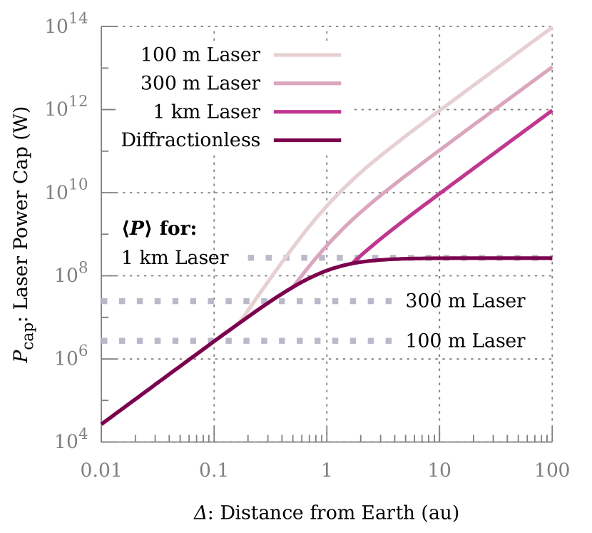
Figure 11: A $2R_{\text{com}}=500$ m diameter comet at $r=r_{\text{cap}}=1$ au intercepts $\sim$3 kW solar radiation. The solid lines indicate the laser power $P=P_{\text{cap}}$ that, in concert with solar illumination, produces this maximum heating at various distances $\Delta$ from the Earth for $L_{\text{las}}=100$ m, 300 m, and 1 km. The “diffractionless” curve represents a hypothetical laser with zero beam divergence, where the entire beam is always intercepted by the comet regardless of $\Delta$. As shown in the graph, $P_{\text{cap}}$ diverges from the diffractionless limit once $\Delta$ is sufficiently large for $R_{\text{spot}}>R_{\text{com}}$. Dotted lines indicate the $\langle P\rangle$ of orbital lasers with $L_{\text{PV}}=L_{\text{las}}$ and $\varepsilon=20\%$. Distance from the Sun, used to compute solar flux, is approximated for this figure as $r=\sqrt{\Delta^{2}+(\text{1 au})^{2}}$.

The stress applied to a comet by sublimation is a complicated function of the comet’s geometry and internal structure—information unlikely to be available for a newly identified comet. Without this information, an accurate prediction of disintegration cannot be developed. When approximating stress as a monotonic function of the total incident radiation, a straightforward method to avoid disintegration is to cap the total power incident on the comet to a level such that the structural integrity of the nucleus is retained. Bortle (1991) empirically estimated this limit, finding that $\sim$70% of ground-observed comets with perihelion distance $q$ and absolute magnitude $H_{0}>7.0+6.0(q/\text{1 au})$ disintegrate. In the absence of a reliable function connecting a comet’s absolute magnitude $H_{0}$ to its radius $R_{\text{com}}$, this relation cannot be directly incorporated into the simulations. The relation does, however, suggest that bright (and therefore, large) comets more readily survive perihelion and are thus more resistant to fragmentation on heating than their fainter counterparts.

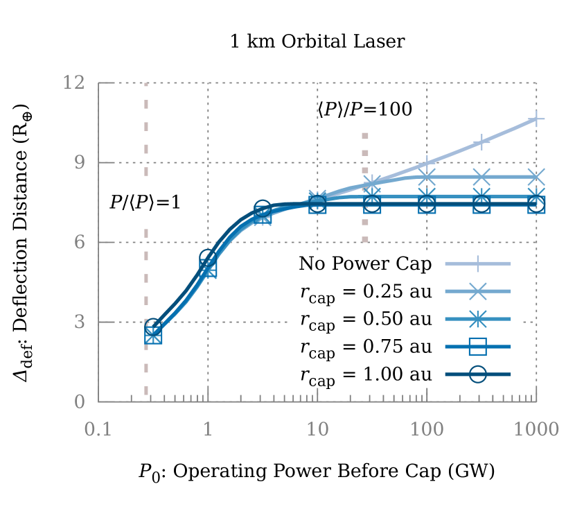
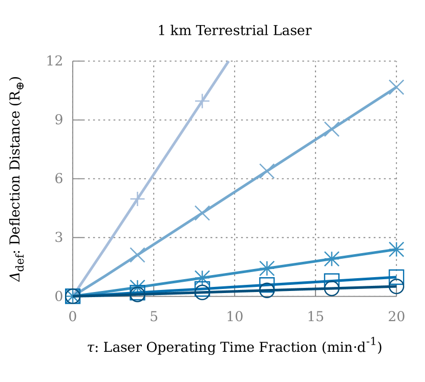
Figure 12: Deflection of the canonical comet over 2 yr with a cap on $P$ for a $L_{\text{las}}=1$ km orbital laser array with $\varepsilon=20\%$ (left) and a $L_{\text{las}}=1$ km, $P=1$ GW terrestrial laser array (right): Even a stringent $r_{\text{cap}}=1$ km only minimally reduces the deflection effectiveness of the orbital laser, as $\langle P\rangle$ is unaffected. In contrast, terrestrial lasers are constrained by $\tau$, so a cap on $P$ also sets a cap on $\langle P\rangle$ which results in a much greater reduction in effectiveness, particularly for large laser arrays.

One strategy could be to restrict laser power to $P\leq P_{\text{cap}}$ where $P=P_{\text{cap}}$ yields a total incident radiation on the comet, from the Sun and laser combined, equivalent to that from the Sun alone at $r=r_{\text{cap}}=1$ au, the largest (and hence, safest) sensible $r_{\text{cap}}$ for avoiding fragmentation during deflection. Any comet that disintegrates at a larger $r>1$ au would disintegrate before reaching Earth, even without the laser. Fig. 11 shows $P_{\text{cap}}$ for a $2R_{\text{com}}=500$ m diameter comet with this $r_{\text{cap}}=1$ au over a range of $\Delta$ for several $L_{\text{las}}$. If impact is set to occur after the comet’s perihelion passage, or if the comet is known to have previously survived perihelion at a distance $q$ from the Sun, a less restrictive $r_{\text{cap}}=q\leq 1$ au may be used instead. Meanwhile, if the comet is very bright ($H_{0}\ll 7.0$), the risk of fragmentation from heating, as determined by Bortle (1991), is sufficient low that a cap on power is unnecessary.

The effects of introducing a $P\leq P_{\text{cap}}$ cap are illustrated in Fig. 12. Such a cap only minimally reduces the effectiveness of a space laser with fixed $\langle P\rangle$. In contrast, ground lasers are constrained by $\tau$, and with fixed $\tau$, a cap on $P$ also sets a cap on $\langle P\rangle$ which produces a much larger reduction in deflection effectiveness. This effect is especially pronounced for large laser arrays, for where the cap is active for comets well beyond the inner solar system. Beginning deflection early—while the comet is still sufficiently far for the cap to be inactive—overcomes this limitation, although doing so would require significant advancement in detection and tracking capability. Alternatively, if fragmentation can be predicted more reliably, a less stringent cap may be used.

Note that, given a sufficiently early discovery and sufficiently large laser, it may still be possible to deflect a comet with an even higher $r_{\text{cap}}>1$ au, such that its trajectory has shifted sufficiently to avoid impact by all fragments before it reaches $r<r_{\text{cap}}$ and fragments from solar heating. Simulating this scenario, however, requires modeling the fragmentation process of a comet nucleus, a process better suited for a more detailed analysis of the general considerations for planetary defense from cometary impacts.

Finally, it is important to recognize that, although these considerations may reduce the likelihood of fragmentation, they will not fully eliminate the risk. The residual risk poses a significant challenge that must eventually be addressed prior to the commencement of deflection. Note also that, depending on the specifics of the threat, fragmentation of the comet nucleus may be preferable to the impact of an intact nucleus. Intentional disruption may be achievable by following the opposite of the strategies above, elevating $P$ to point where the tensile strength of the nucleus is exceeded. Both topics require separate in-depth analyses and will be deferred to future analyses of planetary defense strategy for cometary impactors.

4 Conclusions

Comets pose unique challenges left unanswered by most techniques for mitigating asteroid impact. Comets’ highly eccentric orbits hinder discovery until, at best, a few years before impact. The expected uncertainties in trajectory for a newly discovered object, including in $A$, introduce further delays to a response. The rapid progression from discovery to impact, coupled with often extreme delta-v requirements, renders interception missions either unreliable or otherwise impractical with presently available propulsion technologies.

This lack of attention stems in part from the rarity of comets relative to NEAs. Comets of all groups are estimated to be responsible for less than 1% of all impact events in Earth’s recent geological record, though they may comprise the majority of large impactors of diameter $2R_{\text{com}}\gtrsim 1$ km (Yeomans & Chamberlin, 2013). No comets of any size have been confirmed to have impacted the Earth in the historical past, nor is one expected to impact anytime in the foreseeable future. Hence, the near-term risk posed by comets is far lower than that of asteroids, which are generally smaller but far more common—and have been observed to impact the Earth in recent history.

Even so, given their unpredictable timing and the likely catastrophic global consequences of an impact, comet deflection remains an important consideration in planetary defense strategy. Further attention should be given to the possibility and consequences of comet disintegration during deflection—as well as other unintended consequences, such as dust generation, that may prove fatal to insufficiently shielded satellites in Earth orbit (Beech et al., 1995).

Attention must also be directed toward the engineering challenges of large-scale laser arrays. Unless a strategy is prepared and a system is developed and primed before discovery, impact mitigation will be improbable. However, given adequate preparation, these preliminary simulations suggest that use of large, high-powered laser arrays—either in Earth orbit or, with advancements in adaptive optics technology, on the ground—may prove to be a viable strategy for mitigating comet impacts.

References

- Beech et al. (1995) Beech, M., Brown, P., & Jones, J. 1995, QJRAS, 36, 127
- Boehnhardt (2004) Boehnhardt, H. 2004, in Comets II, ed. M. C. Festou, H. U. Keller, & H. A. Weaver (Tucson, AZ: Univ. of Arizona Press), 301–316
- Bortle (1991) Bortle, J. 1991, ICQ, 13, 89
- Delsemme & Miller (1971) Delsemme, A., & Miller, D. 1971, P&SS, 19, 1229
- Farnocchia et al. (2016) Farnocchia, D., Chesley, S., Micheli, M., et al. 2016, Icarus, 266, 279
- Folkner et al. (2008) Folkner, W., Williams, J., & Boggs, D. 2008, The Planetary and Lunar Ephemeris DE 421, Memorandum IOM 343R-08-003, Jet Propulsion Laboratory
- Foster et al. (2013) Foster, C., Bellerose, J., Mauro, D., & Jaroux, B. 2013, AcAau, 90, 112
- Francis (2005) Francis, P. J. 2005, ApJ, 635, 1348
- Griswold et al. (2015) Griswold, J., Madajian, J., Johansson, I., et al. 2015, in Proc. SPIE, ed. E. W. Taylor & D. A. Cardimona, Vol. 9616, 961606
- Gundlach et al. (2012) Gundlach, B., Blum, J., Skorov, Y. V., & Keller, H. 2012, arXiv:1203.1808
- Hyland et al. (2010) Hyland, D. C., Altwaijry, H. A., Ge, S., et al. 2010, CosRe, 48, 430
- Johansson et al. (2014) Johansson, I., Tsareva, T., Griswold, J., et al. 2014, in Proc. SPIE, ed. E. W. Taylor & D. A. Cardimona, Vol. 9226, 922607
- Kahan & Li (1997) Kahan, W., & Li, R.-C. 1997, MaCom, 66, 1089
- Koenig & Chyba (2007) Koenig, J. D., & Chyba, C. F. 2007, Science and Global Security, 15, 57
- Kopp et al. (2005) Kopp, G., Lawrence, G., & Rottman, G. 2005, SoPh, 230, 129
- Królikowska (2004) Królikowska, M. 2004, A&A, 427, 1117
- Kulkarni et al. (2018) Kulkarni, N., Lubin, P., & Zhang, Q. 2018, AJ, 155, 155
- Lu & Love (2005) Lu, E. T., & Love, S. G. 2005, Natur, 438, 177
- Lubin (2016) Lubin, P. 2016, JBIS, 69, 40
- Lubin et al. (2014) Lubin, P., Hughes, G. B., Bible, J., et al. 2014, OptEn, 53, 025103
- Marsden et al. (1973) Marsden, B. G., Sekanina, Z., & Yeomans, D. 1973, AJ, 78, 211
- McInnes (2004) McInnes, C. R. 2004, P&SS, 52, 587
- Riley et al. (2014) Riley, J., Lubin, P., Hughes, G. B., et al. 2014, in Proc. SPIE, ed. E. W. Taylor & D. A. Cardimona, Vol. 9226, 922606
- Tange (2011) Tange, O. 2011, ;login: The USENIX Magazine, 36, 42
- Vasile & Maddock (2010) Vasile, M., & Maddock, C. A. 2010, CeMDA, 107, 265
- Walker et al. (2005) Walker, R., Izzo, D., de Negueruela, C., et al. 2005, JBIS, 58, 268
- Williams et al. (2017) Williams, T., Kelley, C., & others. 2017, gnuplot 5.0: An Interactive Plotting Program
- Yeomans & Chamberlin (2013) Yeomans, D. K., & Chamberlin, A. B. 2013, AcAau, 90, 3
- Yeomans et al. (2004) Yeomans, D. K., Chodas, P. W., Sitarski, G., Szutowicz, S., & Królikowska, M. 2004, in Comets II, ed. M. C. Festou, H. U. Keller, & H. A. Weaver (Tucson, AZ: Univ. of Arizona Press), 137–151
- Zhang et al. (2016a) Zhang, Q., Lubin, P. M., & Hughes, G. B. 2016a, in Planetary Defense and Space Environment Applications, Vol. 9981, Proc. SPIE, ed. G. B. Hughes, 998108
- Zhang et al. (2017) Zhang, Q., Lubin, P. M., & Hughes, G. B. 2017, in Astronomical Optics: Design, Manufacture, and Test of Space and Ground Systems, Vol. 10401, Proc. SPIE, ed. T. B. Hull, D. W. Kim, & P. Hallibert, 1040104
- Zhang et al. (2016b) Zhang, Q., Walsh, K. J., Melis, C., Hughes, G. B., & Lubin, P. M. 2016b, PASP, 128, 045001