OTOC, complexity and entropy in bi-partite systems

Abstract

There is a remarkable interest in the study of Out-of-time ordered correlators (OTOCs) that goes from many body theory and high energy physics to quantum chaos. In this latter case there is a special focus on the comparison with the traditional measures of quantum complexity such as the spectral statistics, for example. The exponential growth has been verified for many paradigmatic maps and systems. But less is known for multi-partite cases. On the other hand the recently introduced Wigner separability entropy (WSE) and its classical counterpart (CSE) provide with a complexity measure that treats equally quantum and classical distributions in phase space. We have compared the behavior of these measures in a system consisting of two coupled and perturbed cat maps with different dynamics: double hyperbolic (HH), double elliptic (EE) and mixed (HE). In all cases, we have found that the OTOCs and the WSE have essentially the same behavior, providing with a complete characterization in generic bi-partite systems and at the same time revealing them as very good measures of quantum complexity for phase space distributions. Moreover, we establish a relation between both quantities by means of a recently proven theorem linking the second Renyi entropy and OTOCs.

Introduction.–Nowadays there is a huge interest in OTOCs among the quantum chaos community, where they have been related to traditional measures as spectral statistics and the like Qchaos . These correlators were first introduced in superconductivity studies Larkin , where their exponential growth over time was associated to chaotic behavior. As a matter of fact, if we adopt the usual definition of the OTOC given by

$$C(t)=\left\langle[\hat{A}(t),B][\hat{A}(t),B]^{\dagger}\right\rangle,$$ (1)

(i.e., the thermal average $\left\langle\cdot\right\rangle={\rm Tr}(\cdot)/N$ of the commutator between two operators at different times, with $N$ the Hilbert space dimension), and we take $\hat{A}=\hat{X}$ and $\hat{B}=\hat{P}$ as the position and momentum operators respectively, it is easy to show this. The commutator leads to the Poisson bracket at the semiclassical level, which in turn grows exponentially at a rate of twice the Lyapunov exponent. In Garcia , this exponential growth for the (one dimensional) quantum perturbed Arnold cat map has been shown. Also, in Lakshminarayan a growth at half this rate was discovered in the baker map, using projectors instead of position and momentum operators. Finally, there was some controversy around the Bunimovich stadium case in Hashimoto , which has been explained by means of replacing the thermal average with Gaussian minimal uncertainty wavepackets (the “most classical” initial state) Rozenbaum .

But previously the surge in interest came from the many body area Shenker ; Aleiner ; Huang ; Borgonovi . As a prominent feature, an upper bound for the OTOC growth was conjectured in the context of black hole models Maldacena . Also, the OTOCs have been related to multiple quantum coherences and used as an entanglement witness in NMR Gaertner . A path integral approach has been presented, in which the OTOCs are expressed as coherent sums over contributions from different mean field solutions Rammensee . More recently, the OTOC behavior has been determined for one of the simplest examples of multi-particle systems. This corresponds to a bi-partite system consisting of two strongly chaotic and weakly coupled kicked rotors Lakshminarayan2 . It was found that the scrambling process has two phases, one in which the exponential growth is intra subsystem and a second one which only depends on the interaction.

Recently, in the spirit of algorithmic complexity, the Wigner separability entropy (WSE) Benenti and the Classical Separability Entropy (CSE) Prosen have been introduced as measures of complexity that put quantum and classical distributions (in phase space) on an equal footing. We have characterized how the WSE and the CSE behave for a bi-partite system given by two coupled and perturbed cat maps with different dynamics. Three cases were considered, one where both maps are hyperbolic (chaotic) (HH), one where both are elliptic (regular) (EE), and a mixed situation where one map is hyperbolic and the other elliptic (HE) Bergamasco . In this work we have set a twofold objective, on one hand we have investigated the behavior of OTOCs for these different scenarios, and on the other hand we have compared them with the complexity measures previously mentioned. As a result, we have found that the OTOCs are in general good indicators of complexity that can be related to WSE and CSE via the so called OTOC-RE theorem Hosur ; Fan .

OTOCs and WSE.–In Eq. 1 we have defined these correlators in the most commonly found way, i.e. by performing a thermal average of the commutator of two operators, one of which evolves with time in a Heisenberg fashion. For our purposes which are investigating the behavior for different kinds of dynamics in each subsystem it is preferable to calculate the expectation value on a given initial state, much in the same way as we have done previously to compute the phase space entropies WSE and CSE Bergamasco . This is accomplished by $\left\langle\cdot\right\rangle={\rm Tr}(\rho\cdot)$, where $\rho$ is the density matrix of a “classical like” initial state, which we take to be a coherent state.

Also, there is freedom in the choice of operators $\hat{A}$ and $\hat{B}$. As mentioned, we can take $\hat{X}$ and $\hat{P}$ in order to formally associate them to a Lyapunov exponential growth. But we will also consider $\hat{B}=\hat{\rho}(0)$, the density operator of the initial state. The cat map is defined on the torus and we use an approximation to position and momentum operators in the classical limit that makes use of the Schwinger shift operators Schwinger

$$\hat{V}=\sum_{q\in\mathbb{Z_{N}}}{{|q+1\rangle}{\langle q|}}\ ;\ \hat{U}=\sum_{q\in\mathbb{Z_{N}}}{{|q\rangle}{\langle q|}\tau^{2q}}$$ (2)

with $\tau=\exp{i\pi/N}$. Position and momentum operators for each one degree of freedom map can be written as

$$\hat{X}=\frac{\hat{U}-\hat{U}^{\dagger}}{2i}\ ;\ \hat{P}=\frac{\hat{V}-\hat{V}^{\dagger}}{2i}.$$ (3)

These operators are readily extended to the two degrees of freedom bi-partite space as the tensor product of similar operators acting on each subsystem (labeled as $1$ and $2$),

$$\hat{X}^{\rm 2D}=\hat{X}^{1}\otimes\hat{X}^{2}\ ;\ \hat{P}^{\rm 2D}=\hat{P}^{1}\otimes\hat{P}^{2}.$$ (4)

It is worth mentioning that when the operators $\hat{A}$ and $\hat{B}$ are Hermitian the OTOC of Eq. 1 can be expressed as the correlators difference:

$$C(t)=-2[C_{4}(t)-C_{2}(t)]/N,$$ (5)

where $C_{2}(t)={\rm Tr}[\hat{A}^{2}(t)\hat{B}^{2}]$ (a 2 point correlator), and $C_{4}(t)={\rm Tr}[\hat{A}(t)\hat{B}\hat{A}(t)\hat{B}]$ (a 4 point correlator). Also, our ${\rm Tr}(\rho\cdot)$ operation when $\hat{B}=\hat{\rho}(0)$ corresponds to a pure state, can be proven to be equivalent to ${\rm Tr}(\cdot)/2$, making it similar to the thermal average times $N$.

We now briefly explain the WSE and CSE definitions and main properties. A good analogue of Liouville distributions in classical mechanics is given by the Wigner distributions in phase space $W(\bm{x})$, which are defined in terms of the Weyl-Wigner symbol of the density operator as

$$W(\bm{x})=(2\pi\hbar)^{-d/2}\rho(\bm{x})=(2\pi\hbar)^{-d/2}\text{Tr}\left[\hat{R}_{\bm{x}}\hat{\rho}\right],$$ (6)

where $\hat{R}_{\bm{x}}$ forms a basis set of unitary reflection operators on points $\bm{x}\equiv(\bm{q},\bm{p})$ ozrep ; opetor . The Schmidt decomposition of the density operator is given by

$$\hat{\rho}=\sum\sigma_{n}\hat{a}_{n}\otimes\hat{b}_{n},$$ (7)

where $\{\hat{a}_{n}\}$ and $\{\hat{b}_{n}\}$ are orthonormal bases for the Hilbert-Schmidt operator spaces $B(\mathcal{H}_{1})$ and $B(\mathcal{H}_{2})$, respectively. This directly leads to the Schmidt (singular value) decomposition of the Wigner function given by

$$W(\bm{x})=\sum_{n}\sigma_{n}a_{n}(\bm{x_{1}})b_{n}(\bm{x_{2}}),$$ (8)

where $\{a_{n}\}$ and $\{b_{n}\}$ are now orthonormal bases for $L^{2}(\Omega_{1})$ and $L^{2}(\Omega_{2})$ (which are associated to the Hilbert space decomposition), such that:

$$a_{n}(\bm{x_{1}})=\text{Tr}\left[\hat{R}_{\bm{x_{1}}}\hat{a}_{n}\right],\quad\textrm{and}\quad b_{n}(\bm{x_{2}})=\text{Tr}\left[\hat{R}_{\bm{x_{2}}}\hat{b}_{n}\right].$$

The WSE is defined in Benenti as $h[W]=-\sum_{n}\tilde{\sigma}_{n}^{2}\ln\tilde{\sigma}_{n}^{2}$, where $\tilde{\sigma}_{n}\equiv{\sigma_{n}}/{\sqrt{\int d\bm{x}W^{2}(\bm{x})}}.$

The WSE $h[W]$ provides a measure of separability of the Wigner function with respect to a given phase space decomposition. One of the main properties of the WSE is that its classical analogue is the CSE (or s-entropy) $h[\rho_{c}]$ defined in Prosen , where a discretized classical phase space distribution is used instead of the Wigner function $W(\boldmath{x})$. This makes the complexity concept in both the quantum and the classical world fully equivalent. It is very important to mention that for a pure state $\hat{\rho}=|\psi\rangle\langle\psi|$, $h[W]=-2S_{\rm VN}(\hat{\rho}_{1})=-2S_{\rm VN}(\hat{\rho}_{2})$, where $\hat{\rho}_{1}=\text{Tr}_{2}(\hat{\rho})$ and $\hat{\rho}_{2}=\text{Tr}_{1}(\hat{\rho})$ are the reduced density operators for subsystems $1$ and $2$, and $S_{\rm VN}$ is the von Neumann entropy.

Model system.–The quantum cat map Hannay 1980 is paradigmatic in the quantum chaos area Hannay 1980 ; Ozorio 1994 ; Haake ; Espositi 2005 . We consider the behavior of two coupled perturbed cat maps, a two degrees of freedom example. These two maps can have different types of dynamics.

Each degree of freedom is defined on the 2-torus as Hannay 1980

$$\left(\begin{array}[]{c}q_{t+1}\\ p_{t+1}\end{array}\right)=\mathcal{M}\left(\begin{array}[]{c}q_{t}\\ p_{t}+\epsilon\left(q_{t}\right)\end{array}\right)$$ (9)

with $q$ and $p$ taken modulo $1$, and

$$\epsilon\left(q_{t}\right)=-\frac{K}{2\pi}\sin\left(2\pi q_{t}\right).$$

For the ergodic case we have chosen the hyperbolic map

$$\mathcal{M}_{h}=\left(\begin{array}[]{cc}2&1\\ 3&2\end{array}\right),$$ (10)

while for the regular behavior we use the elliptic map

$$\mathcal{M}_{e}=\left(\begin{array}[]{cc}0&1\\ -1&0\end{array}\right).$$ (11)

Torus quantization amounts to have a finite Hilbert space of dimension $N=\frac{1}{2\pi\hbar}$, with discrete positions and momenta in a lattice of separation $\frac{1}{N}$ Hannay 1980 . In coordinate representation the propagator is given by a $N\times N$ unitary matrix

$$U_{jk}=A{\exp}\left[\frac{i\pi}{N\mathcal{M}_{12}}(\mathcal{M}_{11}j^{2}-2jk+\mathcal{M}_{22}k^{2})+F\right],$$ (12)

where $A=[1/\left(iN\mathcal{M}_{12}\right)]^{1/2}$, and $F=[iKN/(2\pi)]\cos(2\pi j/N)$. The states $\langle q|\mathbf{q}_{j}\rangle$ are periodic Dirac delta distributions at positions $q=j/N{\rm mod}(1)$, with $j$ integer in $[0,N-1]$.

The two degrees of freedom classical system is defined in a four-dimensional phase space of coordinates $\left(q^{1},q^{2},p^{1},p^{2}\right)$ Benenti as

$$\left(\begin{array}[]{c}q_{t+1}^{1}\\ p_{t+1}^{1}\end{array}\right)=\mathcal{M}_{1}\left(\begin{array}[]{c}q_{t}^{1}\\ p_{t}^{1}+\epsilon\left(q_{t}^{1}\right)+\kappa\left(q_{t}^{1},q_{t}^{2}\right)\end{array}\right)$$

and

$$\left(\begin{array}[]{c}q_{t+1}^{2}\\ p_{t+1}^{2}\end{array}\right)=\mathcal{M}_{2}\left(\begin{array}[]{c}q_{t}^{2}\\ p_{t}^{2}+\epsilon\left(q_{t}^{2}\right)+\kappa\left(q_{t}^{1},q_{t}^{2}\right)\end{array}\right).$$

The coupling between both maps is chosen to be $\kappa(q_{t}^{1},q_{t}^{2})=-(K_{c}/2\pi)\sin(2\pi q_{t}^{1}+2\pi q_{t}^{2})$. The corresponding two degrees of freedom quantum evolution is given by the tensor product of the one degree of freedom maps, a $N^{2}\times N^{2}$ unitary matrix $U_{j_{1}j_{2},k_{1}k_{2}}^{2D}=U_{j_{1}k_{1}}U_{j_{2}k_{2}}C_{j_{1}j_{2}},$ with the coupling matrix (diagonal in the coordinate representation)

$$C_{j_{1}j_{2}}=\exp\left\{\left(\frac{iNK_{c}}{2\pi}\right)\cos\left[\frac{2\pi}{N}\left(j_{1}+j_{2}\right)\right]\right\},$$

where $j_{1},j_{2},k_{1},k_{2}\in\{0,\ldots,N-1\}$. We fix $K=0.25$ and $K_{c}=0.5$ (Anosov condition Ozorio 1994 ), and $N=2^{6}$.

Results.–In order to reach our twofold objective we have investigated the evolution of OTOCs much in the same way we have done in Bergamasco , that is we have evaluated their behavior for 3 different dynamics. First, we consider the EE case. The initial (pure) state is constructed by placing a coherent state on each tori, both centered at $(q,p)=(0.5,0.5)$. This is a fixed point of the hyperbolic and elliptic maps. In Fig. 1 we show the evolution of two OTOCs for $\hat{A}=\hat{X}^{\rm 2D}$, having $\hat{B}=\hat{P}^{\rm 2D}$ in one case, and $\hat{B}=\hat{\rho}(0)$ in the other, as a function of the map time steps. Also we can see the evolution of the linear entropy $S_{\rm L}=1-{\rm Tr}\rho_{1,2}^{2}$, which is a linear approximation to the von Neumann entropy $S_{\rm VN}$. We clearly see the same qualitative behavior, reflecting the lack of complexity growth due to the nature of the dynamics of both maps. We observe the same small oscillations indicative of the rotation of the distributions which remain localized Bergamasco . Both OTOCs have been rescaled in Fig. 1 (and all subsequent Figures) in order to make a comparison. In the inset we display the log-linear version, where no initial exponential growth can be identified for this case.

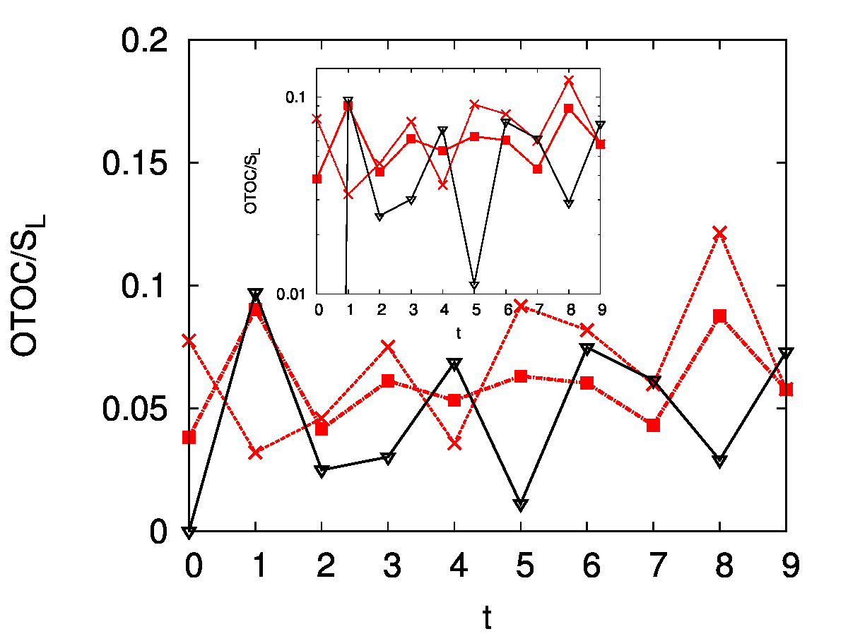
Figure 1: (Color online) Evolution of the linear entropy $S_{L}$ ((black) solid line with down triangles), and rescaled OTOCs for $\hat{A}=\hat{X}^{\rm 2D}$, with $\hat{B}=\hat{P}^{\rm 2D}$ ((red) dashed line with crosses), and $\hat{B}=\hat{\rho}(0)$ ((red) dot-dashed line with squares), as a function of time $t$ (map time steps). $N=2^{6}$, EE maps case with initial coherent state centered at $(q,p)=(0.5,0.5)$. Inset: log-linear version.

It is interesting to see if the OTOC is able to detect the high sensitivity to the region of phase space at which the initial condition is located for the EE case, as we have previously seen by means of the WSE Bergamasco . In fact, this is the case, and also the qualitative behavior is the same for the 3 quantities displayed in Fig. 2. There are clearly more fluctuations in the OTOCs, this will be explained later. Moreover, in the inset it can be checked that no exponential growth is present. Despite this and fluctuations, the previously identified inflection point where quantum effects become important at $t\simeq 10$ Bergamasco is roughly detected by the OTOCs.

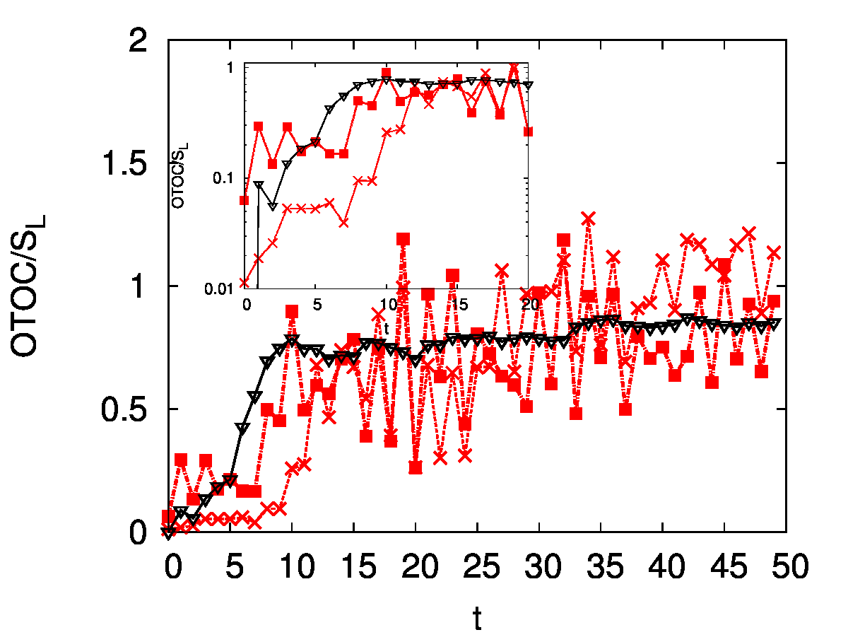
Figure 2: (Color online) Evolution of the linear entropy $S_{L}$ ((black) solid line with down triangles), and rescaled OTOCs for $\hat{A}=\hat{X}^{\rm 2D}$, with $\hat{B}=\hat{P}^{\rm 2D}$ ((red) dashed line with crosses), and $\hat{B}=\hat{\rho}(0)$ ((red) dot-dashed line with squares), as a function of time $t$ (map time steps). $N=2^{6}$, EE maps case with initial coherent state centered at $(q,p)=(\pi/4,\pi/4)$. Inset: log-linear version.

We continue with the HE map case shown in Fig. 3, which again shows a good qualitative agreement between the linear entropy and the OTOCs behavior. The growth is slower for the correlators at early times, resembling more the von Neumann case which we will see in the following. Looking at the inset we cannot clearly identify an initial exponential growth of the correlators. Nevertheless the saturation behavior is very similar and this shows that the OTOC detects the main feature of the mixed dynamics scenario that we have already seen with the WSE: just one hyperbolic degree of freedom suffices to reach maximum complexity (this is accomplished for $t\simeq 200$, not shown here).

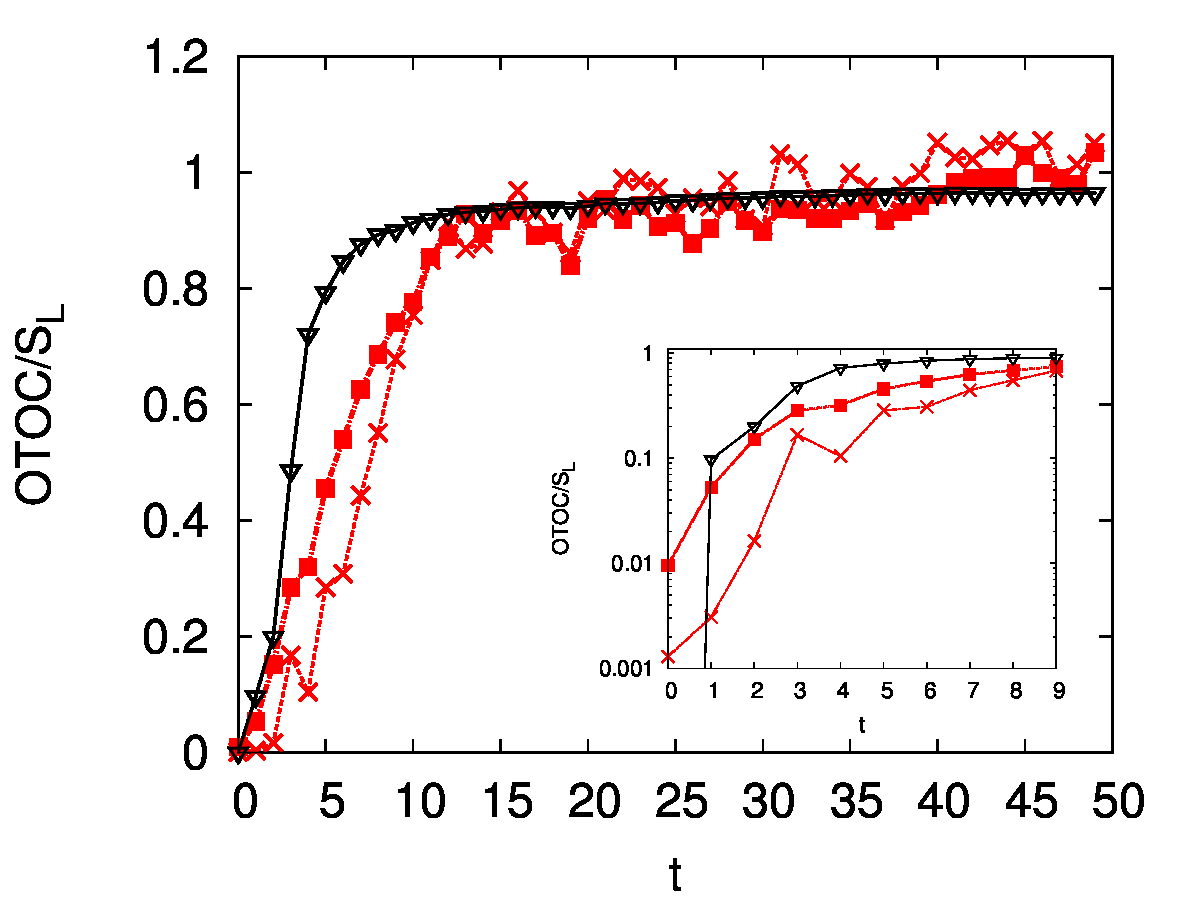
Figure 3: (Color online) Evolution of the linear entropy $S_{L}$ ((black) solid line with down triangles), and rescaled OTOCs for $\hat{A}=\hat{X}^{\rm 2D}$, with $\hat{B}=\hat{P}^{\rm 2D}$ ((red) dashed line with crosses), and $\hat{B}=\hat{\rho}(0)$ ((red) dot-dashed line with squares), as a function of time $t$ (map time steps). $N=2^{6}$, HE maps case with initial coherent state centered at $(q,p)=(0.5,0.5)$. Inset: log-linear version.

Finally, we turn to analyze the HH case, which has also been considered in Lakshminarayan2 very recently. Again, the agreement between OTOCs and $S_{\rm L}$ is remarkable, the $\hat{B}=\hat{\rho}(0)$ case being extremely good. If we look at the inset we can identify an initial exponential growth in full coincidence with previous studies.

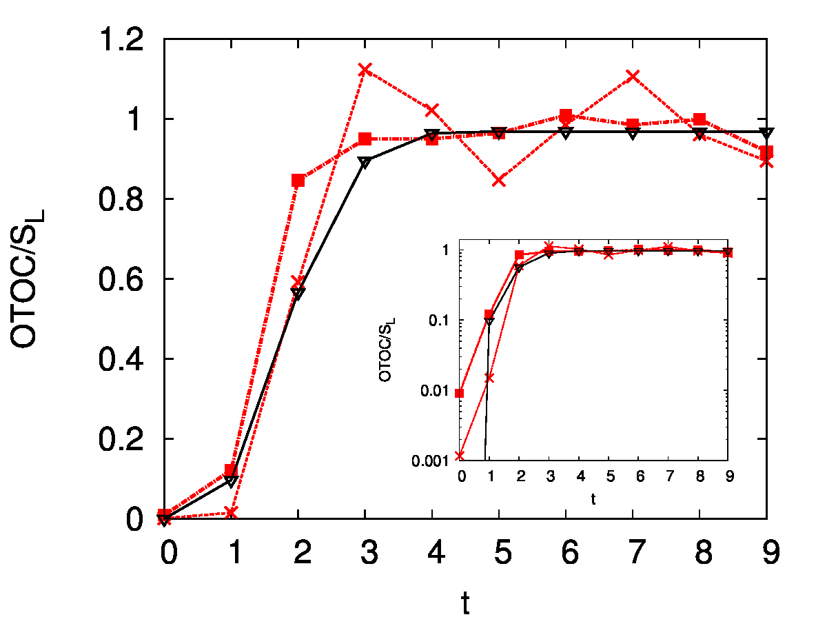
Figure 4: (Color online) Evolution of the linear entropy $S_{L}$ ((black) solid line with down triangles), and rescaled OTOCs for $\hat{A}=\hat{X}^{\rm 2D}$, with $\hat{B}=\hat{P}^{\rm 2D}$ ((red) dashed line with crosses), and $\hat{B}=\hat{\rho}(0)$ ((red) dot-dashed line with squares), as a function of time $t$ (map time steps). $N=2^{6}$, HH maps case with initial coherent state centered at $(q,p)=(0.5,0.5)$. Inset: log-linear version.

But how can we explain this striking similarity between two seemingly different quantities, one coming from a global phase space analysis, and the other being a correlation related to a semiclassical interpretation based on local dynamics? An answer comes from the so called OTOC-RE theorem Hosur ; Fan . It establishes an equivalence between a sum of OTOCs (in fact, the sum of the 4 point correlator in which the OTOC can be split when the operators are Hermitian) over a complete basis of one of the subsystems (the operator that does not evolve is taken to be the initial state $\hat{\rho}(0)$), and the exponential of the second Renyi entropy. This result is usually expressed in the following shape:

$${\rm exp}{-S_{1}^{(^{\prime}2^{\prime})}}=\sum_{\hat{M}\in 2}\left\langle\hat{M}(t)\hat{\rho}(0)\hat{M}(t)\hat{\rho}(0)\right\rangle$$ (13)

where $S_{1}^{(^{\prime}2^{\prime})}=-\log{\rm Tr}_{1}\hat{\rho}_{1}^{2}$ is the second Renyi entropy, the sum runs over a complete basis of subspace $2$, and the usual thermal average is performed. It is easy to see that ${\rm exp}{-S_{1}^{(^{\prime}2^{\prime})}}={\rm Tr}\rho_{1}^{2}$. In the OTOC Eq. 5, we have a 2 point correlator term that in general can be considered to be constant (see for example Garcia ; Lakshminarayan ; Lakshminarayan2 , for chaotic cases). Hence, the OTOC becomes approximately proportional to $1-{\rm Tr}\rho_{1}^{2}$, which is $S_{\rm L}$. Typically there are more oscillations in the OTOCs than in the linear entropy since we only consider one operator $\hat{A}(t)$ that belongs to both subspaces and not the complete basis of one of them as the OTOC-RE theorem prescribes. The equivalence expressed in this theorem is an indicator of an average behavior of which our calculation is a fluctuation.

In order to establish a complete link between the OTOCs and the WSE we show the rescaled von Neumann entropy evolution for the previous 4 cases, together with the linear entropy. We have rescaled $S_{\rm VN}$ in order to better compare it with $S_{\rm L}$ (in the last 2 cases we use the RMT saturation value Lakshminarayan3 ). It becomes clear that $S_{\rm L}$ behaves much in the same way as $S_{\rm VN}$, despite being a linear approximation. It is worth mentioning that for the HE case (Fig. 5 c)) the OTOC initial growth is closer to $S_{\rm VN}$. This will be investigated in the future.

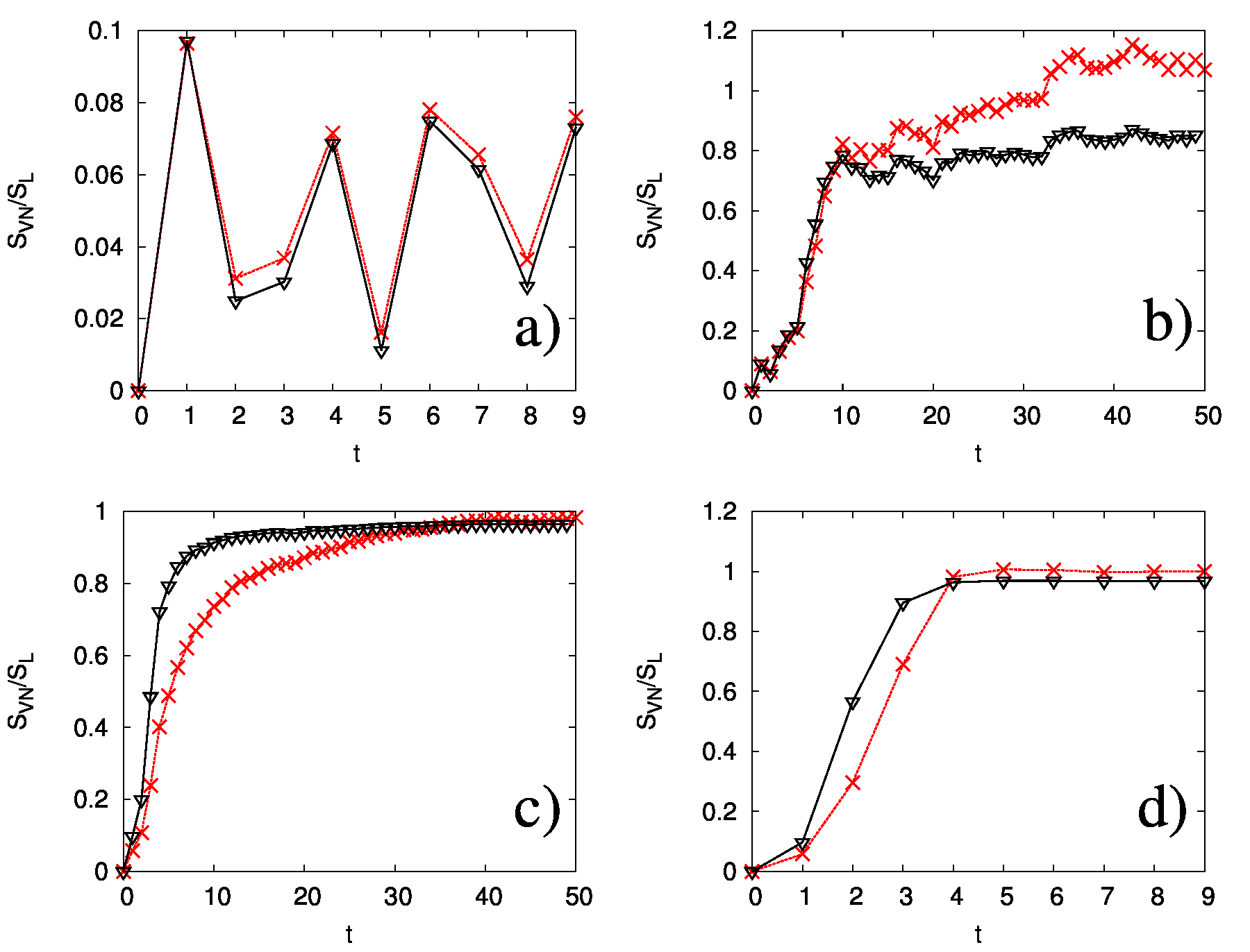
Figure 5: (Color online) Comparison of rescaled von Neumann entropy $S_{\rm VN}$ ((red) dashed line with crosses) with the linear entropy $S_{\rm L}$ ((black) solid line with down triangles) behavior as a function of time $t$ (map time steps). In a) we show the EE case with initial coherent state at $(q,p)=(0.5,0.5)$, in b) the EE case with $(q,p)=(\pi/4,\pi/4)$, in c) the HE case with $(q,p)=(0.5,0.5)$, and in d) the HH case with $(q,p)=(0.5,0.5)$. In all panels $N=2^{6}$.

Conclusions–Interest in OTOCs has grown very fast in the last couple of years, mainly motivated by their power to characterize quantum chaotic manifestations that could have important consequences in many body and high energy physics. In turn, the quantum chaos community is looking at its previous contributions from a new point of view. A third component comes from information theory which has established a precise connection between OTOCs and the second Renyi entropy via the OTOC-RE theorem.

On the other hand, much has been done in one degree of freedom systems regarding OTOC measures but less is known in multi-partite cases. We have investigated a bi-partite system consisting of two coupled and perturbed cat maps with different dynamical scenarios, them being regular and chaotic. In all cases we have found that the behavior of OTOCs (semiclassically related to local measures of chaos) is qualitatively similar to that of the WSE. This latter is a complexity measure defined globally in phase space that treats the quantum and the classical distributions in the same way. This connection is formally explained by means of the equivalence between von Neumann/linear entropy and OTOCs when one of the operators considered is the initial density matrix. By choosing a pure initial state the WSE can be identified with the entropies. On the other hand, the OTOC-RE theorem describes the average behavior of the correlators for any choice of the evolving operator. In fact, even when considering the canonical $\hat{P}$ operator as the non evolving one, the agreement is very good, allowing to generalize this connection.

It is worth mentioning that in many body systems the generic scenario involves chaotic and regular components. We have seen that one chaotic degree of freedom is enough for the complexity measures to reach their maximum prescribed by RMT. However, exponential growth of the OTOCs for localized initial conditions is absent if there is one regular degree of freedom. In Maldacena a bound is set for the OTOC Lyapunov exponential growth in black holes. In our examples we observe that any symmetry (constant of the motion) implies non exponential growth for the entropy. The consequences of this should be carefully explored.

In the future we will investigate the OTOC-RE theorem and WSE connection in order to formalize it for generic initial states and operators. Different symmetry groups will be considered to obtain predictions on specific systems.

Support from CONICET is gratefully acknowledged.

References

- (1) F. Borgonovi, F.M. Izrailev, and L.F. Santos, arXiv:1903.09175 (2019); B. Yan, L. Cincio, and W.H. Zurek, arXiv:1903.02651 (2019).
- (2) A.I. Larkin and Yu.N. Ovchinnikov, Sov. Phys. JETP 28, 1200 (1969).
- (3) I. García-Mata, M. Saraceno, R.A. Jalabert, A.J. Roncaglia, and D.A. Wisniacki, Phys. Rev. Lett. 121, 210601 (2018).
- (4) A. Lakshminarayan, arXiv:1810.12029 (2018).
- (5) K. Hashimoto, K. Murata, and R. Yoshii, J. High Energy Phys. 10 (2017) 138.
- (6) E.B. Rozenbaum, S. Ganeshan, and V. Galitski, arXiv:1801.10591 (2018).
- (7) S.H. Shenker and D. Stanford, J. High Energy Phys. 03 (2014) 067.
- (8) I.L. Aleiner, L. Faoro, and L.B. Ioffe, Ann. Phys. (Amsterdam) 375, 378 (2016).
- (9) Y, Huang, Y.-L. Zhang, and X. Chen, Ann. Phys. (Berlin) 529, 1600318 (2017).
- (10) F. Borgonovi and F. M. Izrailev, arXiv:1806.00435 (2018).
- (11) J. Maldacena, S.H. Shenker, and D. Stanford, J. High Energy Phys. 08 (2016) 106.
- (12) M. G artner, P. Hauke, and A.M. Rey, Phys. Rev. Lett. 120, 040402 (2018).
- (13) J. Rammensee, J.D. Urbina, and K. Richter, Phys. Rev. Lett. 121, 124101 (2018).
- (14) R. Prakash and A. Lakshminarayan, arXiv:190406482 (2019).
- (15) G. Benenti, G.G. Carlo, and T. Prosen, Phys. Rev. E, 85, 051129 (2012).
- (16) T. Prosen, Phys. Rev. E, 83, 031124 (2011).
- (17) P.D. Bergamasco, G.G Carlo, and A.M.F. Rivas, Phys. Rev. E, 96, 062144 (2017).
- (18) P. Hosur, X.L. Qi, D.A. Roberts, and B. Yoshida, J. High Energy Phys. 02 (2016) 004.
- (19) R. Fan, P. Zhang, H. Shen, and H. Zhai, Sci. Bull. 62, 707 (2017).
- (20) J. Schwinger, Proc. Natl. Acad. Sci. U.S.A. 46, 570 (1960).
- (21) A.M. Ozorio de Almeida, Phys. Rep. 295, 266 (1998).
- (22) A.M.F. Rivas and A.M. Ozorio de Almeida, Ann. Phys. 276, 223 (1999).
- (23) J.H. Hannay and M.V. Berry, Physica D 1, 267 (1980).
- (24) M. Basilio De Matos and A.M. Ozorio De Almeida, Ann. Phys. 237, 46 (1995).
- (25) F. Haake, Quantum Signatures of Chaos (Springer-Verlag, New York, 2001).
- (26) M. Degli Espositi and B. Winn, J. Phys. A: Math. Gen. 38, 5895 (2005).
- (27) J.N. Bandyopadhyay and A. Lakshminarayan, Phys. Rev. Lett. 89, 060402 (2002).