Asymptotic regime for impropriety tests of complex random vectors

Abstract

Impropriety testing for complex-valued vectors has been considered lately due to potential applications ranging from digital communications to complex media imaging. This paper provides new results for such tests in the asymptotic regime, i.e. when the vector dimension and sample size grow commensurately to infinity. The studied tests are based on invariant statistics named impropriety coefficients. Limiting distributions for these statistics are derived, together with those of the Generalized Likelihood Ratio Test (GLRT) and Roy’s test, in the Gaussian case. This characterization in the asymptotic regime allows also to identify a phase transition in Roy’s test with potential application in detection of complex-valued low-rank subspace corrupted by proper noise in large datasets. Simulations illustrate the accuracy of the proposed asymptotic approximations.

I Introduction

Testing for properness consists of deciding whether $N$-dimensional complex random vector ${\bf z}\in{\mathbb{C}}^{N}$ is proper or improper. Let us recall that a complex vector ${\bf z}$ is called circular when ${\bf z}$ is equal in distribution to $e^{\bm{i}\theta}{\bf z}$ (i.e. the distribution of ${\bf z}$ is invariant by a rotation of angle $\theta$ in the complex domain [1, 2]). Circularity for Gaussian complex vectors is actually called properness. The problem of testing weither a complex Gaussian vector is proper or not has several potential applications in signal processing and has been considered by several authors, using different means, including Generalized Likelihood Ratio Tests (GLRT) [3, 4], locally most powerful (LMP) test [5, Chapter 3] or frequency domain tests [6]. The asymptotic behavior of GLRT was studied for large sample sizes in the case of random variables ($N=1$) [7] or small/fixed values of $N$ [8]. The situation where both the dimension of the complex vector and the size of the sample tend to infinity was not considered until our recent preliminary study [9]. This article formalizes and extends [9], therefore filling a gap and provides insight into the asymptotic behavior of impropriety test when the vector dimension and sample size grow commensurately to infinity. Practical applications of this asymptotic regime occur for example in communications when a large number of dense arrays are deployed, i.e. for massive MIMO [10] and cognitive radio [11], as well as in fMRI [12] or phase retrieval and imaging in complex media [13].

Central to many of the tests available in the literature, the set of invariant parameters was first considered in [14], allowing for the derivation of invariant statistics used in [8]. Invariant parameters are in one-to-one correspondence with canonical correlation coefficients [4] as explained in [5], and referred to as impropriety coefficients [15].

In this article, we consider $N$-dimensional complex-valued centered random vectors with Cartesian form such as ${\bf z}={\bf u}+\bm{i}{\bf v}$, i.e. ${\bf u}$ and ${\bf v}$ are $N$-dimensional real vectors with zero mean, i.e. ${\bf u}\in{\mathbb{R}}^{N}$, ${\bf v}\in{\mathbb{R}}^{N}$, and ${\mathbb{E}}[{\bf u}]={\mathbb{E}}[{\bf v}]={\bf 0}$. Two augmented representations are classically used in the literature to study complex vectors ${\bf z}\in{\mathbb{C}}^{N}$, namely the real augmented representation ${\bf x}$ and the complex augmented representation $\tilde{\bf z}$. The former consists of representing ${\bf z}\in{\mathbb{C}}^{N}$ by a twice larger real-valued vector ${\bf x}=\left[{\bf u}^{T},{\bf v}^{T}\right]^{T}\in{\mathbb{R}}^{2N}$ made up from the real and imaginary parts of ${\bf z}$, while the latter consists of using a twice larger complex-valued vector $\tilde{\bf z}=\left[{\bf z}^{T},{\bf z}^{*T}\right]^{T}\in{\mathbb{C}}^{2N}$ containing ${\bf z}$ and its conjugate ${\bf z}^{*}$. Both representations are equivalent and easily connected using linear mappings given for example in [5]. In this paper, we make use of the real representation ${\bf x}\in{\mathbb{R}}^{2N}$.

Recalling that ${\mathbb{E}}[{\bf z}]={\bf 0}$, and thus that ${\mathbb{E}}[{\bf x}]={\bf 0}$, second order statistics of ${\bf z}\in{\mathbb{C}}^{N}$ are contained in the real-valued covariance matrix ${\bf C}\in{\mathbb{R}}^{2N\times 2N}$ of the real representation vector ${\bf x}$, which reads:

$${\mathbb{E}}[{\bf x}{\bf x}^{T}]={\bf C}=\begin{pmatrix}{\bf C}_{{\bf u}{\bf u}}&{\bf C}_{{\bf u}{\bf v}}\\ {\bf C}_{{\bf v}{\bf u}}&{\bf C}_{{\bf v}{\bf v}}\\ \end{pmatrix}$$ (1)

where ${\bf C}_{{\bf a}{\bf b}}\in{\mathbb{R}}^{N\times N}$ denotes the real-valued (cross)covariance matrix between real vectors ${\bf a}$ and ${\bf b}$, and with ${\bf C}_{{\bf b}{\bf a}}={\bf C}_{{\bf a}{\bf b}}^{T}$. A complex-valued Gaussian vector ${\bf z}\in{\mathbb{C}}^{N}$ is called proper iff the following two conditions hold:

$$\begin{array}[]{lcr}{\bf C}_{{\bf u}{\bf u}}={\bf C}_{{\bf v}{\bf v}}&\text{and}&{\bf C}^{T}_{{\bf u}{\bf v}}=-{\bf C}_{{\bf u}{\bf v}}.\end{array}$$ (2)

If these conditions are not fulfilled, then ${\bf z}$ is called improper. Properness thus means that real and imaginary parts, i.e. ${\bf u}$ and ${\bf v}$, have the same covariance matrix and their cross-covariance is skew-symmetric (2). When using the complex representation, properness is equivalent to having ${\mathbb{E}}[{\bf z}{\bf z}^{T}]={\bf 0}$, which means that ${\bf z}$ and ${\bf z}^{*}$ are uncorrelated. Note that even in the Gaussian case, ${\bf z}$ and ${\bf z}^{*}$ can not be independent (they are related by a one-to-one deterministic application) even being uncorrelated. Thus, the statistical problem of measuring the impropriety of complex-valued vectors is by nature different from standard canonical correlation analysis where the two Gaussian vectors are independent when their canonical correlation coefficients are zero. This emphasizes why state-of-the-art results from multivariate analysis such as canonical correlation analysis, or more recent works to test the independence between complex random vectors [16, 17] or the diagonality of the covariance matrix [18], cannot be extended in an easy manner to impropriety testing.

The original contributions of the present work consist of the following results in the asymptotic high-dimensional regime: the limiting distribution of the maximal invariant statistics, and accurate approximations for standard test statistics used in multivariate analysis, namely the GLRT and Roy’s test, are derived under the null hypothesis of properness. Moreover, a phase transition behavior is shown to exist, allowing for the detection of complex-valued low-rank signals (modeled as complex vectors) corrupted by proper noise.

The paper is organized as follows. In Section II, the maximal invariant statistics are introduced for impropriety testing. Their limiting distributions are also derived. Section III provides the exact and limiting distributions of GLRT, as well as the limiting distributions of Roy’s test statistics. Some simulations are conducted in IV to appreciate the accuracy of the proposed approximations. The relation with canonical correlation analysis results is discussed in Section V. Some concluding remarks are given in the last section.

II Impropriety coefficients

In order to design tests based on second order statistics and that are not sensitive to reparametrization (by linear transformation), it is known [14, 5] that the impropriety coefficients should be the quantities to use. In this section, we introduce them and provide joint and marginal distributions in the asymptotic regime for their empirical estimates.

II-A Testing problem

In many applications such as fMRI [19], DOA estimation [20] or communications [5], it is common use to model the vector of interest, denoted ${\bf z}$, as being improper and corrupted by proper Gaussian noise. Consequently, statistical tests have been proposed to investigate the impropriety of a complex vector given a sample (of size $M$ in the sequel), from which one needs to decide:

$$\begin{cases}H_{0}:&${\bf z}$\textrm{ is {\em proper} {\color[rgb]{0,0,1}iff} condition \eqref{eq:prop} holds,}\\ H_{1}:&${\bf z}$\textrm{ is {\em improper} otherwise.}\end{cases}$$ (3)

In order to design a statistical test which is invariant under linear transformation, and as explained in [14], one should use the eigenvalues of the augmented covariance matrix ${\bf C}$ given in (1). Before introducing the invariant statistics to be derived from observed complex vectors, we first recall some results about the eigenvalues of real augmented PSD (Positive Semi-Definite) matrices.

II-B Invariant parameters

Let $\mathcal{G}$ be the set of non-singular matrices ${\bf G}\in\mathbb{R}^{2N\times 2N}$ s.t.

$${\bf G}=\begin{pmatrix}{\bf G}_{1}&-{\bf G}_{2}\\ {\bf G}_{2}&{\bf G}_{1}\end{pmatrix},$$

where ${\bf G}_{1},{\bf G}_{2}\in\mathbb{R}^{N\times N}$. Let $\mathcal{S}$ be the set of all $2N\times 2N$ real positive definite symmetric matrices. According to the test formulation (3) and condition (2), the null hypothesis $H_{0}$ is equivalent to ${\bf C}\in\mathcal{T}=\mathcal{S}\cap\mathcal{G}$.

As explained in [14], $\mathcal{G}$ is a group (isomorphic to the group $GL_{N}(\mathbb{C})$ of non-singular $N\times N$ complex matrices under the mapping ${\bf G}\leftrightarrow{\bf G}_{1}+\bm{i}{\bf G}_{2}$), with the matrix multiplication as the group operation. Moreover $\mathcal{G}$ acts transitively on $\mathcal{T}$ under the action $({\bf G},{\bf T})\in\mathcal{G}\times\mathcal{T}\mapsto{\bf G}{\bf T}{\bf G}^{T}\in\mathcal{T}$. Thus, a parametric characterization of $H_{0}$ should be invariant to this group action: the value of the parameters to be tested should be the same for ${\bf C}$ and ${\bf G}{\bf C}{\bf G}^{T}$ for any ${\bf G}\in\mathcal{G}$.

Next, we introduce a decomposition for any ${\bf C}\in\mathcal{S}$ that was originally given in [14] and reads:

$${\bf C}=\dot{{\bf C}}+\ddot{{\bf C}}$$ (4)

where

$$\dot{{\bf C}} =\frac{1}{2}\begin{pmatrix}{\bf C}_{{\bf u}{\bf u}}+{\bf C}_{{\bf v}{\bf v}}&{\bf C}_{{\bf u}{\bf v}}-{\bf C}_{{\bf v}{\bf u}}\\ {\bf C}_{{\bf v}{\bf u}}-{\bf C}_{{\bf u}{\bf v}}&{\bf C}_{{\bf u}{\bf u}}+{\bf C}_{{\bf v}{\bf v}}\end{pmatrix}\in\mathcal{G},$$

$$\ddot{{\bf C}} =\frac{1}{2}\begin{pmatrix}{\bf C}_{{\bf u}{\bf u}}-{\bf C}_{{\bf v}{\bf v}}&{\bf C}_{{\bf u}{\bf v}}+{\bf C}_{{\bf v}{\bf u}}\\ {\bf C}_{{\bf u}{\bf v}}+{\bf C}_{{\bf v}{\bf u}}&{\bf C}_{{\bf v}{\bf v}}-{\bf C}_{{\bf u}{\bf u}}\end{pmatrix}.$$

Using this decomposition, one can define the following $2N\times 2N$ real symmetric matrix

$${\bf\Gamma}({\bf C}) =\dot{{\bf C}}^{-\frac{1}{2}}\ddot{{\bf C}}\dot{{\bf C}}^{-\frac{1}{2}}.$$ (5)

It is now possible to give the following lemma about the parametrization of ${\bf C}$.

Lemma 1 (Invariant parameters [14]).

Any matrix ${\bf C}\in\mathcal{S}$ can be written as:

$${\bf C}={\bf G}\begin{pmatrix}{\bf I}_{N}+{\bf D}_{\lambda}&0\\ 0&{\bf I}_{N}-{\bf D}_{\lambda}\end{pmatrix}{\bf G}^{T},$$

where ${\bf G}\in\mathcal{G}$, ${\bf I}_{N}$ is the $N\times N$ identity matrix and ${\bf D}_{\lambda}=\mathrm{diag}(\lambda_{1},\ldots,\lambda_{N})$ is an $N\times N$ diagonal matrix whose diagonal entries denoted as $\lambda_{n}$, for $1\leq n\leq N$, are the non-negative eigenvalues of the $2N\times 2N$ matrix ${\bf\Gamma}({\bf C})$ given in (5). They satisfy the following properties:

1. $\lambda_{n}$ and $-\lambda_{n}$, for $1\leq n\leq N$, form the set of eigenvalues of ${\bf\Gamma}({\bf C})$,

2. $\lambda_{n}\in[0,1]$ with, by convention, the following ordering $1\geq\lambda_{1}\geq\ldots\geq\lambda_{N}\geq 0$.

Proof.

See [14, lemma 5.1 and 5.2]. ∎

Lemma 1 shows that any invariant parameterization of the covariance matrix ${\bf C}$ for the group action of $\mathcal{G}$ depends only on the $N$ (non-negative) eigenvalues $1\geq\lambda_{1}\geq\ldots\geq\lambda_{N}\geq 0$ of ${\bf\Gamma}({\bf C})$. Thus these eigenvalues are termed maximal invariant parameters [21, Chapter 6]. Moreover under the null hypothesis $H_{0}$, one has that $\lambda_{1}=\ldots=\lambda_{N}=0$ as $\ddot{{\bf C}}$ reduces to the zero matrix according to (2). Within the invariant parameterization, the testing problem in (3) becomes:

$$\begin{cases}H_{0}:&\lambda_{1}=0,\\ H_{1}:&\lambda_{1}>0,\end{cases}$$ (6)

where the alternative hypothesis $H_{1}$ means that there exists at least one positive eigenvalue. Note that the invariance property ensures that the test does not depend on the (common) representation basis of the real and imaginary parts of ${\bf z}$, i.e. vectors $\bf u$ and $\bf v$. Also, $\lambda_{n}$, the eigenvalues of $\Gamma({\bf C})$, are directly related to the ones obtained using the complex augmented representation, i.e. based on the complex covariance matrix:

$${\mathbb{E}}[\tilde{\bf z}\tilde{\bf z}^{\dagger}] =\begin{pmatrix}{\bf C}_{{\bf z}{\bf z}}&{\bf C}_{{\bf z}{\bf z}^{*}}\\ {\bf C}_{{\bf z}^{*}{\bf z}}&{\bf C}_{{\bf z}^{*}{\bf z}^{*}}\\ \end{pmatrix},$$

where $.^{\dagger}$ stands for transposition and conjugation, and ${\bf C}_{{\bf r}{\bf s}}={\mathbb{E}}[{\bf r}{\bf s}^{\dagger}]$ denotes the (complex) cross-covariance between the sized $N$ complex vectors ${\bf r}$ and ${\bf s}$. In fact, as detailed in [5, Chapter 3] and [8, 15], the eigenvalues $\lambda_{n}$, for $1\leq n\leq N$, are also the square roots of the eigenvalues of the following $N\times N$ complex matrix:

$${\bf C}_{{\bf z}^{*}{\bf z}^{*}}^{-1}{\bf C}_{{\bf z}^{*}{\bf z}}{\bf C}_{{\bf z}{\bf z}}^{-1}{\bf C}_{{\bf z}{\bf z}^{*}}$$ (7)

Matrix (7) corresponds to the usual population canonical correlation matrix to derive the canonical variables between two vectors, here the complex ones ${\bf z}$ and ${\bf z}^{*}$. Hence the squared eigenvalues $\lambda_{n}^{2}$ are commonly referred to as the canonical correlation coefficients. In our specific framework of impropriety testing, these coefficients are also known as circularity coefficients [22, 23], or impropriety coefficients [15]. In the sequel, to better emphasize the statistical differences between our impropriety testing problem with the problem of testing the independence between two vectors, we will make use of the name population impropriety coefficients for the eigenvalues $\lambda_{n}$. The sample version of these eigenvalues (derived from the sample covariances) will be will be denoted as $l_{n}$ and $r_{n}\equiv l_{n}^{2}$ for their squared values, and referred to as the sample impropriety coefficients and the sample squared impropriety coefficients respectively.

II-C Invariant statistics

Consider a sample of size $M$, denoted ${\bf X}=\left\{{\bf x}_{m}\right\}_{m=1}^{M}$, where ${\bf x}_{m}=[{\bf u}^{T}_{m},{\bf v}^{T}_{m}]^{T}$ are $2N$-dimensional i.i.d. Gaussian real vectors with zero mean and covariance matrix ${\bf C}$. In the Gaussian framework, a sufficient statistics is given by the $2N\times 2N$ sample covariance matrix:

$${\bf S} =\begin{pmatrix}{\bf S}_{{\bf u}{\bf u}}&{\bf S}_{{\bf u}{\bf v}}\\ {\bf S}_{{\bf v}{\bf u}}&{\bf S}_{{\bf v}{\bf v}}\\ \end{pmatrix},$$ (8)

with ${\bf S}_{{\bf a}{\bf b}}\in{\mathbb{R}}^{N\times N}$ the real-valued sample (cross)covariance matrix of real vectors $\left\{{\bf a}_{m}\right\}_{m=1}^{M}$ and $\left\{{\bf b}_{m}\right\}_{m=1}^{M}$ such that:

$${\bf S}_{{\bf a}{\bf b}}=\frac{1}{M}\sum_{m=1}^{M}{\bf a}_{m}{\bf b}_{m}^{T}.$$ (9)

We assume here that $M\geq 2N$, thus ${\bf S}$ belongs to the real symmetric positive definite matrices set $\mathcal{S}$. According to the previous section, since $H_{0}$ is invariant under the action of the group $\mathcal{G}$, an invariant test statistic must only depend on the $N$ non-negative eigenvalues $l_{n}$, $1\leq n\leq N$, of

$${\bf\Gamma}({\bf S})=\dot{{\bf S}}^{-\frac{1}{2}}\ddot{{\bf S}}\dot{{\bf S}}^{-\frac{1}{2}}.$$ (10)

These sample impropriety coefficients obey $1\geq l_{1}\geq\ldots\geq l_{N}\geq 0$ according to Lemma 1, and are an estimate of the population impropriety coefficients $\lambda_{n}$ obtained from the population covariance ${\bf C}$. Note that all the $\lambda_{n}$ are zero under the null hypothesis $H_{0}$, and at least one is non-negative otherwise. As a consequence, the distribution of the $l_{n}$ should be stochastically greater under $H_{1}$ than under $H_{0}$. All invariant test can be derived from this property. A key point to derive now a tractable statistical test procedure is to characterize the null distribution of these sample impropriety coefficients.

II-D Eigenvalue distribution under $H_{0}$

Let $\mathcal{B}_{N}(\frac{1}{2}n_{1},\frac{1}{2}n_{2})$ denote the $N\times N$-dimensional matrix variate beta distribution with parameters $n_{1}$ and $n_{2}$ as defined for instance in [24, definition 3.3.2, p. 110]. It is possible to obtain, under $H_{0}$, the joint probability density function (pdf) of the squared eigenvalues of $\Gamma({\bf S})$ in terms of this matrix-variate beta distribution.

Proposition 2 (Joint distribution of impropriety coefficients).

Under $H_{0}$, the vector $(r_{1},\ldots,r_{N})$ of the sample squared impropriety coefficients $r_{n}\equiv l_{n}^{2}$, for $1\leq n\leq N$, is distributed as the eigenvalues of the matrix-variate beta distribution $\mathcal{B}_{N}(\frac{1}{2}n_{1},\frac{1}{2}n_{2})$, with parameters $n_{1}=N+1$ and $n_{2}=M-N$. Moreover, the joint pdf of $(r_{1},\ldots,r_{N})$ is expressed as:

$$p(r_{1},\ldots,r_{N})\propto\prod_{n=1}^{N}(1-r_{n})^{(M-2N-1)/2}\prod_{k<n}^{N}(r_{k}-r_{n}),$$ (11)

where $1\geq r_{1}\geq\ldots\geq r_{N}\geq 0$.

Proof.

As shown in [14, pp. 39-41], the sample eigenvalue vector $(l_{1},\ldots,l_{N})$ is characterized by the following pdf:

$$p(l_{1},\ldots,l_{N})\propto\prod_{n=1}^{N}(2l_{n})(1-l_{n}^{2})^{(M-2N-1)/2}\prod_{k<n}^{N}(l_{k}^{2}-l_{n}^{2}).$$

A simple change of variables yields the pdf of $(r_{1},\ldots,r_{N})$ given in (11). Moreover, according to [24, Theorem 3.3.4, p. 112], (11) is the pdf of the eigenvalues of the matrix variate beta distribution $\mathcal{B}_{N}(\frac{N+1}{2},\frac{M-N}{2})$, which concludes the proof. ∎

It is interesting to note that the pdf given in Proposition 2 is close to what would be obtained if one would perform a canonical correlation analysis on ${\bf z}$ and ${\bf z}^{*}$ considered as $N$-dimensional real Gaussian independent vectors. Here vectors ${\bf z}$ and ${\bf z}^{*}$ are actually complex valued and fully dependent. This is further discussed in Section V.

Expression (11) gives, under the $H_{0}$ hypothesis, the joint distribution of the squared sample impropriety coefficients $(r_{1},\ldots,r_{N})$. In the general case, obtaining an analytic expression of marginal distributions of individual eigenvalues is a complicated task. However, in the asymptotic regime, i.e. when the dimension $N$ and the number of samples $M$ go to infinity while their ratio stays commensurable, one can obtain those marginal laws. The following theorem gives the distribution of one (unordered) sample impropriety coefficient in this regime.

Theorem 3 (Limiting empirical distribution).

As $M,\,N\,\rightarrow\,\infty$ with the ratio $M/N\,\rightarrow\,\gamma\in[2,+\infty)$ being finite, the marginal empirical distribution of the unordered sample squared impropriety coefficients (i.e. the squared eigenvalues of ${\bf\Gamma}({\bf S})$) converges, under the $H_{0}$ hypothesis, to the probability measure with density:

$$f(r) =\frac{1}{2\pi(1-r)}\sqrt{4(\gamma-1)\tfrac{1-r}{r}-(\gamma-2)^{2}},$$ (12)

on its support $r\in(0,c)$, with $c=\tfrac{4(\gamma-1)}{\gamma^{2}}\in(0,1]$.

Proof.

See Appendix A. ∎

Corollary 4 (Moments).

The mean and variance of the limiting distribution under $H_{0}$ of a sample squared impropriety coefficients are expressed respectively as ${1}/{\gamma}$ and ${(\gamma-1)}/{\gamma^{3}}$.

Proof.

Expressions of these limiting moments can be derived directly from the pdf (12) by symbolic computation. ∎

A few remarks are in order:

• When $\gamma\rightarrow+\infty$, the expression of the mean and variance emphasizes that the sample impropriety coefficients converge to zero, which are the population values under $H_{0}$. This is the usual behavior in small dimension when $N$ is fixed while $M$ tends to infinity.

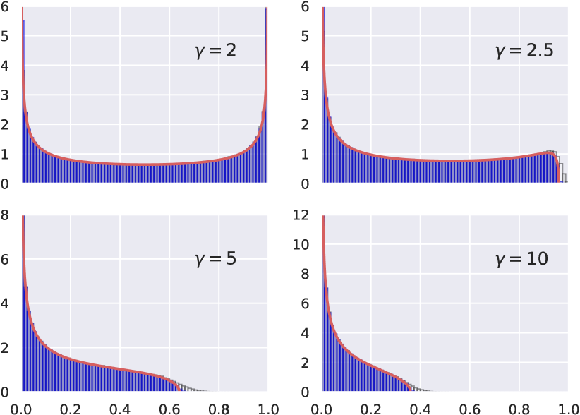
• Conversely, in the special case where $\gamma=2$, the asymptotic null distribution of the squared sample impropriety coefficients is $\mathcal{B}(\frac{1}{2},\frac{1}{2})$, known as the arcsine law. In this limiting case, the sample impropriety coefficients are symmetrically distributed on $[0,1]$ around $1/2$ with two symmetric modes at the edges (even if the population impropriety coefficients are zero).

III Testing for impropriety

In this section, we make use of the results from Proposition 2 and Theorem 3 to introduce the asymptotic behavior of two impropriety tests: the classical GLRT and Roy’s test (based on the largest eigenvalue of the ${\bf\Gamma}({\bf S})$ matrix).

III-A GLRT

III-A1 Expression of the GLRT statistic

A very classical procedure to test for impropriety is obtained from the Generalized Likelihood Ratio Test (GLRT) statistic defined as:

$$T\propto\frac{\stackrel{{\scriptstyle[}}{{\bf C}}\textrm{ s.t. $H_{0}$}]{\sup}\quad p({\bf X}\,;\,{\bf C})}{\stackrel{{\scriptstyle[}}{{\bf C}}\textrm{ s.t. $H_{1}$}]{\sup}\quad p({\bf X}\,;\,{\bf C})},$$

where $p({\bf X}\,;\,{\bf C})$ is the multivariate normal pdf of the sample ${\bf X}$ composed of $M$ i.i.d. $2N$-dimension real Gaussian vectors with zero mean and covariance matrix ${\bf C}$. Under $H_{1}$, ${\bf C}\in\mathcal{S}$ is a symmetric definite positive matrix. Its maximum likelihood (ML) estimate is the sample covariance ${\bf S}$. Under $H_{0}$, one has that ${\bf C}=\dot{{\bf C}}$ so that ${\bf C}\in\mathcal{T}$. Then the ML estimate of ${\bf C}$ under $H_{0}$ reduces to $\dot{{\bf S}}$, as shown for instance in [14]. The testing problem in (3) can thus be rephrased:

$$\begin{cases}H_{0}:&{\bf C}\in\mathcal{T},\\ H_{1}:&{\bf C}\in\mathcal{S}.\end{cases}$$ (13)

Actually, the GLRT statistic is expressed as:

$$T =|{\bf S}|/|\dot{{\bf S}}|,$$

$$=|\dot{{\bf S}}^{\frac{1}{2}}\left({\bf I}_{2N}+{\bf\Gamma}({\bf S})\right)\dot{{\bf S}}^{\frac{1}{2}}|/|\dot{{\bf S}}|=\left|{\bf I}_{2N}+\Gamma({\bf S})\right|,$$

$$=\prod_{n=1}^{N}(1+l_{n})(1-l_{n})=\prod_{n=1}^{N}(1-r_{n}),$$ (14)

where the first line is due to the Gaussian pdf expression; the second line comes from the decomposition ${\bf S}=\dot{{\bf S}}+\ddot{{\bf S}}$ and the expression (10) of ${\bf\Gamma}({\bf S})$; the third line comes from Lemma 1, where $r_{n}=l_{n}^{2}$, $1\leq n\leq N$, are the sample squared impropriety coefficients. As explained previously, it is important to note that the GLRT is invariant: the resulting statistics given in (14) only depends on the eigenvalues of ${\bf\Gamma}({\bf S})$.

III-A2 Distribution under the hypothesis $H_{0}$

Let $\Lambda(d,m,n)$ denote Wilks lambda distribution, with dimension parameter $d$ and degrees of freedom parameters $m$ and $n$, as defined for instance in [25, definition 3.7.1, p. 81].

Theorem 5.

The GLRT statistics $T$ given in (14) is distributed under $H_{0}$ as the following Wilks lambda distribution:

$$T\sim\Lambda(N,M-N,N+1).$$

Moreover this statistics can be expressed under $H_{0}$ as:

$$T=\prod_{n=1}^{N}u_{n},$$ (15)

where the $u_{n}$ are independent beta-distributed random variables such that $u_{n}\sim\mathcal{B}\left(\frac{M-N-n+1}{2},\frac{N+1}{2}\right)$, for $1\leq n\leq N$.

Proof.

According to Proposition 2, the $r_{n}$ in (14) are distributed as the eigenvalues of the matrix variate beta distribution $\mathcal{B}_{N}(\frac{1}{2}n_{1},\frac{1}{2}n_{2})$ with parameters $n_{1}=N+1$ and $n_{2}=M-N$. Using the mirror symmetry property of the beta distribution, the $(1-r_{n})$ are distributed as the eigenvalues of the random matrix ${\bf U}\sim\mathcal{B}_{N}(\frac{1}{2}n_{2},\frac{1}{2}n_{1})$. According now to [24, Theorem 3.3.3, p. 110], ${\bf U}$ can be decomposed as ${\bf U}={\bf\Theta}^{T}{\bf\Theta}$ where ${\bf\Theta}$ is upper triangular with diagonal entries $\theta_{nn}$ that are independent and where $u_{n}\equiv\theta_{nn}^{2}\sim\mathcal{B}\left(\frac{n_{2}-n+1}{2},\frac{n_{1}}{2}\right)$ for $1\leq n\leq N$. This concludes the proof since $T=|{\bf U}|=\prod_{n=1}^{N}\theta_{nn}^{2}$. ∎

Equation (15) gives also a more efficient way to sample from the null distribution of $T$ in $O(N)$ independent draws, as it is actually not required to generate the $2N\times 2N$ sample covariance matrix ${\bf S}$, nor to compute the eigenvalues of ${\bf\Gamma}({\bf S})$.

III-A3 High-dimensional asymptotic distribution under $H_{0}$

The characterization given in (15) allows us to derive, under the null hypothesis $H_{0}$, an asymptotic distribution for the GLRT statistic $T$ in the high dimensional (i.e. large $N$) case. This yields a simple tractable closed form approximation of the considered Wilks lambda distribution when both the dimension $N$ and the sample size $M$ are large.

Theorem 6 (Central limit theorem in high dimension).

Let $T^{\prime}=-\ln T$ where $T$ is the GLRT statistic given in (14). Assume that $M,\,N\,\rightarrow\,\infty$ so that the ratio $M/N\,\rightarrow\,\gamma\in(2,+\infty)$. Under $H_{0}$, the following asymptotic normal distribution is obtained for $T^{\prime}$:

$$\frac{1}{s}\left(T^{\prime}-m\right)\ {\xrightarrow{d}}\ \mathcal{N}(0,1)$$ (16)

where

$$m =M\left[\ln\frac{\gamma}{\gamma-1}+\frac{\gamma-2}{\gamma}\ln\frac{\gamma-2}{\gamma-1}\right]+\frac{1}{2}\ln\frac{\gamma}{\gamma-2},$$

$$s^{2} =2\left[\ln\frac{(\gamma-1)^{2}}{\gamma(\gamma-2)}+\frac{1}{M}\frac{1}{\gamma-2}\right].$$

Proof.

See Appendix B. ∎

Bartlett derived a classical approximation for Wilks lambda distribution [25, p. 94] in a low-dimensional setting. This gives, when the dimension $N$ is fixed while $M$ goes to infinity, the same asymptotic distribution as obtained in [8]:

$$-(M-N)\ln T\ {\xrightarrow{d}}\ \chi^{2}_{N(N+1)},$$ (17)

where $\chi^{2}_{N(N+1)}$ denotes the chi-squared distribution with $N(N+1)$ degrees of freedom. Note that this approximation was used recently in [26], in a high-dimensional setting in the absence of better approximation.

Using Theorem 6, the Bartlett approximation can now be adjusted to cover both the low and high-dimensional cases. Let $\mathcal{G}\left(q,p\right)$ denote the gamma distribution with pdf $f(x)\propto x^{q-1}e^{-x/p}$, where $q$ and $p$ are the shape and scale parameters respectively.

Corollary 7 (Adjusted Bartlett approximation).

Let $\gamma=M/N>2$, then the log-GLRT statistics $T^{\prime}=-\ln(T)$ can be approximated as a shifted gamma distribution:

$$\frac{1}{s}\left(T^{\prime}-\alpha\right)\approx\mathcal{G}\left(q,p\right),$$ (18)

with

$$q =N(N+1)/2,\quad p=\sqrt{1/q},\quad\alpha=m-pqs,$$

and $m$ and $s^{2}$ are defined in Theorem 6, and where $\approx$ stands for pointwise equivalence of distribution functions for large $M$ under both the low dimensional, i.e. $N$ is fixed and small w.r.t. $M$, or the high dimensional, i.e. $N$ has order of $M$, regime.

Proof.

In the high dimensional setting, under the assumptions of Theorem 6, the gamma distribution $\mathcal{G}\left(q,p\right)$ converges towards the normal one as the shape parameter $q$ goes to infinity. Since the mean and variance of $T^{\prime}$ are the same for the shifted gamma approximation (18) and the normal one (16), they are asymptotically equivalent.

In the low-dimensional setting where $N$ is fixed while $M$ goes to infinity, one gets that $p$ and $q$ are fixed, $\alpha/s\rightarrow 0$, and $ps=\frac{2}{N(\gamma-1)}+O\left(1/\gamma^{2}\right)=\frac{2}{M-N}+O(1/M^{2})$. Moreover, in this limiting case, $T^{\prime}{\xrightarrow{d}}0$ according to the decomposition given in (15). Thus $\frac{1}{s}\left(T^{\prime}-\alpha\right)=\frac{p}{2}(M-N)T^{\prime}+o(1)$. Because $\chi^{2}_{q}=\frac{2}{p}\mathcal{G}\left(q,p\right)$, (18) means that $(M-N)T^{\prime}$ is asymptotically $\chi^{2}_{q}$ distributed. This is the Bartlett limiting distribution (17), which is known to be valid in this low dimensional asymptotic regime ∎

III-B Roy’s test

In multivariate statistics, Roy’s test is a well known procedure to detect the alternate hypothesis $H_{1}$ for which at least one eigenvalue is non-zero. This test relies on the statistics of the largest eigenvalue [25, p. 84] or, equivalently in our case, the statistics of the largest squared impropriety coefficients $r_{1}=l_{1}^{2}$. The principle is to reject the $H_{0}$ hypothesis as soon as $r_{1}>\eta_{\alpha}$, where the threshold $\eta_{\alpha}$ is tuned according to the law of $r_{1}$ under the $H_{0}$ hypothesis together with the nominal control level $\alpha$ (probability of false alarm).

Theorem 8 (Limiting null distribution for Roy’s test).

As $M,\,N\,\rightarrow\,\infty$ such that the ratio $M/N\,\rightarrow\,\gamma\in[2,+\infty)$ is finite, let $W=\log{(r_{1}/(1-r_{1}))}$ be the logit transform of the largest impropriety coefficient $r_{1}$. Under $H_{0}$, the asymptotic law of $W$ converges towards a first order Tracy-Widom law denoted as $\mathcal{TW}_{1}$:

$$\frac{W-\mu}{\sigma}\,\rightarrow\mathcal{TW}_{1},$$ (19)

with

$$\mu =2\log\tan\left(\tfrac{\varphi+\psi}{2}\right),$$

$$\sigma^{3} =\frac{16}{M^{2}}\frac{1}{\sin^{2}(\varphi+\psi)\sin\psi\sin\varphi},$$

$$\psi =\arccos{\left(\tfrac{M-2N+1}{M}\right)},$$

$$\varphi =\arccos{\left(\tfrac{M-2N-1}{M}\right)}.$$

Proof.

This is a direct result of proposition 2 and the asymptotic law of the largest eigenvalue of a $\mathcal{B}_{N}(\frac{1}{2}n_{1},\frac{1}{2}n_{2})$ matrix-variate distribution given in [27]. ∎

The variable $W$ being expressed as an increasing function of $r_{1}$, Roy’s test is equivalent to $W$ and the Theorem 8 allows for the calibration of the test. It should be noted that [28] proposes a procedure to evaluate the exact (not asymptotic) law of $W$. Nevertheless, the simple approximation by the $\mathcal{TW}_{1}$ law is in practice sufficiently precise for most cases as long as the dimension is large enough (e.g. typically for $N\geq 10$).

III-C Spiked impropriety model

Recently, spiked models involving complex valued vectors have been found to nicely describe multiplexed phase retrieval problems in complex media imaging [13]. Here, we provide theoretical results related to the phase transition behavior occurring in such models. Spiked models are special sparse cases for the alternative hypothesis $H_{1}$. They assume that the rank of the population matrix is low and remains fixed in the high-dimensional asymptotic regime. For the impropriety test setting, this means that the number $k$ of non-zero eigenvalues of $\bf\Gamma(\bf S)$, or equivalently $\ddot{\bf C}$, is fixed. An example, which corresponds to a low-rank improper signal corrupted by proper noise, is given in Section IV-B2.

Theorem 9 (Phase transition threshold).

Assume that there exist $k$ non-zero population impropriety coefficients $\lambda_{1}\geq\cdots\geq\lambda_{k}>0$, and $\lambda_{k+1}=\cdots=\lambda_{N}=0$ where $k$ is fixed. Under the assumptions of Theorem 3, we have the following convergence for the square of the largest impropriety coefficient $r_{n}$ with $1\leq n\leq k$,

$$\textrm{ if }\lambda_{n}^{2}\leq\rho_{c},\qquad r_{n} \stackrel{{\scriptstyle a.s.}}{{\longrightarrow}}c,$$

$$\textrm{If }\lambda_{n}^{2}>\rho_{c},\qquad r_{n} \stackrel{{\scriptstyle a.s.}}{{\longrightarrow}}\overline{\rho}_{n},$$

where

$$\rho_{c} =\frac{1}{\gamma-1},\quad\overline{\rho}_{n}=\lambda_{n}^{2}\left(\frac{\gamma-1}{\gamma}+\frac{1}{\gamma\lambda_{n}^{2}}\right)^{2},$$ (20)

are respectively the phase transition threshold and the limiting values, and $c$ is the edge of the limiting distribution of the bulk defined in Theorem 3.

Proof.

This follows from Proposition 2 and from results for high dimensional limiting distribution of spiked models with Beta distributed matrices given in [29, see Theorem 1.8], or [30]. ∎

Theorem 9 shows that when the spikes are weaker than a given phase transition threshold $\rho_{c}$, none of the sample impropriety coefficients separate from the bulk. This makes the testing problem challenging, and Roy’s test would be powerless in this case. Conversely, for spikes $\lambda_{n}^{2}$ larger than $\rho_{c}$, is is easy to check that $\overline{\rho}_{n}>c$. These sample impropriety coefficients separate now from the bulk, and Roy’s test is expected to be very powerful.

IV Simulations

This section starts with simulations validating the accuracy of the asymptotic distributions derived under the properness hypothesis $H_{0}$. Then, impropriety testing is illustrated under different alternative $H_{1}$ hypotheses: i) equi-correlated model ($N$ non-zero identical impropriety coefficients $\lambda_{1}=\cdots=\lambda_{N}=\rho>0$), ii) spiked model ($\lambda_{1}>0$ while $\lambda_{2}=\cdots=\lambda_{N}=0$) and iii) a mixed model (first half of impropriety coefficients $\lambda_{1},\ldots,\lambda_{[N/2]}>0$ gradually decreases, and the other half is zero). Note that, in the following simulations, we make use, for the sake of readability, of the following abuse of notation: $\gamma$ will now denote the ratio $M/N$ in the considered approximations rather that its limit.

IV-A Empirical distribution of impropriety coefficients

IV-A1 Empirical vs limiting distributions

In order to illustrate the accuracy of Theorem 3 in various settings (including small vector dimensions), Fig. 1 displays, for different values of $N$ and $\gamma$, the empirical distribution of the squares of the sample impropriety coefficients under the properness assumption $H_{0}$. This shows the very good agreement with the limiting empirical distribution derived in Theorem 3. Note that, when $N=10$, small fluctuations can be observed (gray bars) around the right edge $c$ of the limiting empirical distribution. But in a larger dimension ($N=100$), the greatest coefficients converged well towards this edge.

Figure 1: Histograms of the squared sample impropriety coefficients under $H_{0}$ for different values of $\gamma$: blue bars are for $N=100$, gray bars are for $N=10$. The pdf of the limiting distribution given in theorem 3 is shown in solid red line. Histograms obtained with $1000$ Monte-Carlo runs.

IV-A2 Distribution of the GLRT statistic

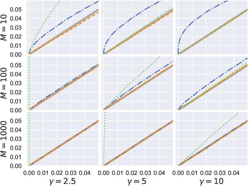
Fig. 2 depicts, for different values of $M$ and $\gamma$, a probability-probability plot of the theoretical null distribution of $T$ against each one of these asymptotic approximations. A deviation from the $y=x$ line indicates a difference between the theoretical and the asymptotic distributions. This shows that, as expected for high-dimensional setting (e.g., $\gamma\leq 5$) and/or large sample sizes (e.g., $M\geq 1000$), the asymptotic log-normal distribution derived in Theorem 6 becomes very accurate and much better than the Bartlett approximation. In addition, the adjusted Bartlett approximation obtained in Corollary 7 is very accurate in all cases (low/high-dimension or small/large sample size). This latter corrects and generalizes the classical Bartlett approximation that may behave poorly even for small (e.g. $N=4$) dimensional vectors, as we can see in the top-left subplot ($M=10$, $\gamma=2.5$) of Fig. 2. The adjusted approximation is therefore of practical interest to calibrate the GLRT procedure according to a nominal significance level.

Figure 2: Comparison, for different values of $\gamma$ and $M$, of asymptotic approximations for the GLRT statistics $T$: $\Pr(T>q_{\alpha})$ under $H_{0}$ vs the nominal control level $\alpha$ in $[0,0.05]$ where $q_{\alpha}$ is the $1-\alpha$ quantile either for the log-normal approximation given in Theorem 6, shown in dashdotted blue line, or the adjusted Bartlett approximation given in Corollary 7, shown in dashed orange line, or the standard Bartlett approximation (17), shown in dotted green line. The solid gray line represents the $y=x$ values. Probabilities estimated with $10^{6}$ Monte-Carlo runs.

IV-A3 Distribution of the Roy’s statistic

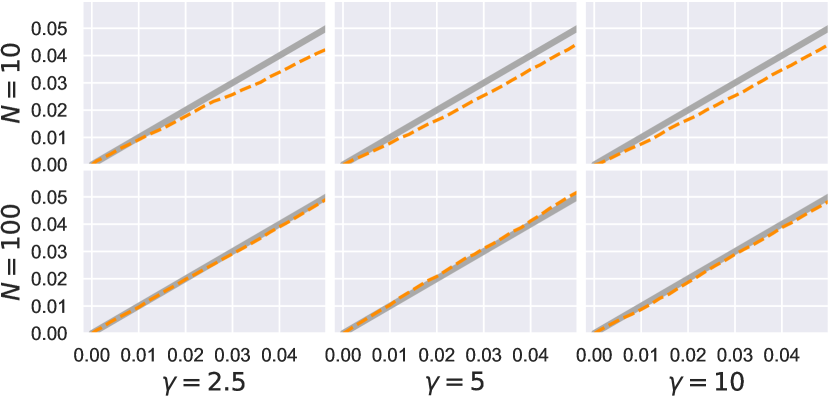
Fig. 3 depicts, for different values of $N$ and $\gamma$, a probability-probability plot of the theoretical null distribution for the largest impropriety coefficients statistics $r_{1}$ , or equivalently its logit-transform $W$, against the asymptotic approximation given in Theorem 8 . This shows that even for a moderate dimension ($N=10$), the Tracy-Widom approximation is quite accurate, and becomes very accurate for a larger dimension ($N=100$).

Figure 3: Comparison, for different values of $\gamma$, of asymptotic approximations for the Roy’s statistics $W$: $\Pr(W>q_{\alpha})$ under $H_{0}$ vs the nominal control level $\alpha$ in $[0,0.05]$ where $q_{\alpha}$ is the $1-\alpha$ quantile for the Tracy-Widom approximation given in Theorem 8, shown in dashed orange line. The solid gray line represents the $y=x$ values. Probabilities estimated with $10^{6}$ Monte-Carlo runs.

IV-B Some impropriety tests scenarios

IV-B1 Equal impropriety coefficients

The case where the population impropriety coefficients are all non-zero and equal, hereinafter referred to as equi-correlated model, can be obtained when the real and imaginary parts have a common contribution:

$$\begin{split}{\bf u}_{m}&={\bf s}_{m}+\sqrt{\theta}{\bf q}_{m},\\ {\bf v}_{m}&={\bf t}_{m}+\sqrt{\theta}{\bf q}_{m},\end{split}$$ (21)

where $\theta>0$, ${\bf s}_{m}$, ${\bf t}_{m}$ and ${\bf q}_{m}$ are i.i.d. Gaussian vectors in $\mathbb{R}^{N}$, for $1\leq m\leq M$. Straightforward computations show that the non-negative roots of ${\bf\Gamma({\bf C})}$, i.e the population impropriety coefficients $\lambda_{1},\ldots,\lambda_{N}$, are all equal to $\lambda\equiv\frac{\theta}{1+\theta}$.

Figure 4: Power of Roy’s test, solid line, and GLRT, dashdotted line, vs the squared population impropriety coefficients $\lambda^{2}$ under the equi-correlated model described in (21), for different values of $\gamma$: blue lines for $\gamma=2.5$, green for $\gamma=5$, orange for $\gamma=10$ (dimension $N=100$, nominal value of false alarm probability $\alpha=0.01$). Powers estimated with $1000$ Monte-Carlo runs.

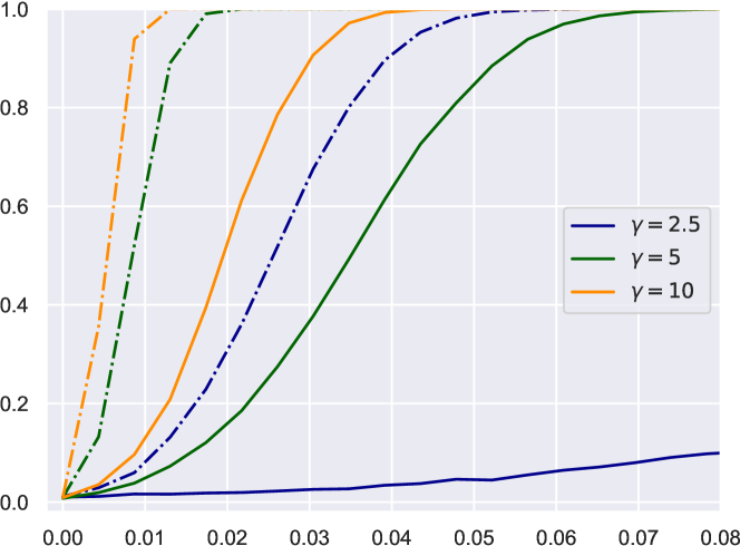
Fig. 4 displays the power of both GLRT and Roy’s test, under the alternative $H_{1}$ obtained for this equi-correlated model, as a function of the impropriety level $\lambda^{2}$. As expected, the GLRT, which uses information from all sample impropriety coefficients, is here much more powerful than Roy’s test, especially in the high dimension case ($\gamma=2.5$) where $M$ and $N$ are close.

IV-B2 Spiked model

A Gaussian spike model with a single non-zero impropriety coefficient can be obtained when the real and imaginary parts have a common contribution of rank one:

$$\begin{split}{\bf u}_{m}&={\bf s}_{m}+\sqrt{\theta}w_{m}\bm{\varphi},\\ {\bf v}_{m}&={\bf t}_{m}+\sqrt{\theta}w_{m}\bm{\varphi},\end{split}$$ (22)

where $\theta>0$, $\bm{\varphi}\in\mathbb{R}^{N}$ is a normed deterministic vector $||\bm{\varphi}||_{2}=1$, $w_{m}$ are i.i.d. Gaussian centered random variables with unit variance, and ${\bf s}_{m}$, ${\bf t}_{m}$ are Gaussian i.i.d. vectors in $\mathbb{R}^{N}$, for $1\leq m\leq M$. This scenario depicts a case where a low-rank improper signal is corrupted by proper noise. Straightforward computations show that there is a single non-zero population impropriety coefficient, a spike, which expresses as $\lambda_{1}=\frac{\theta}{1+\theta}$.

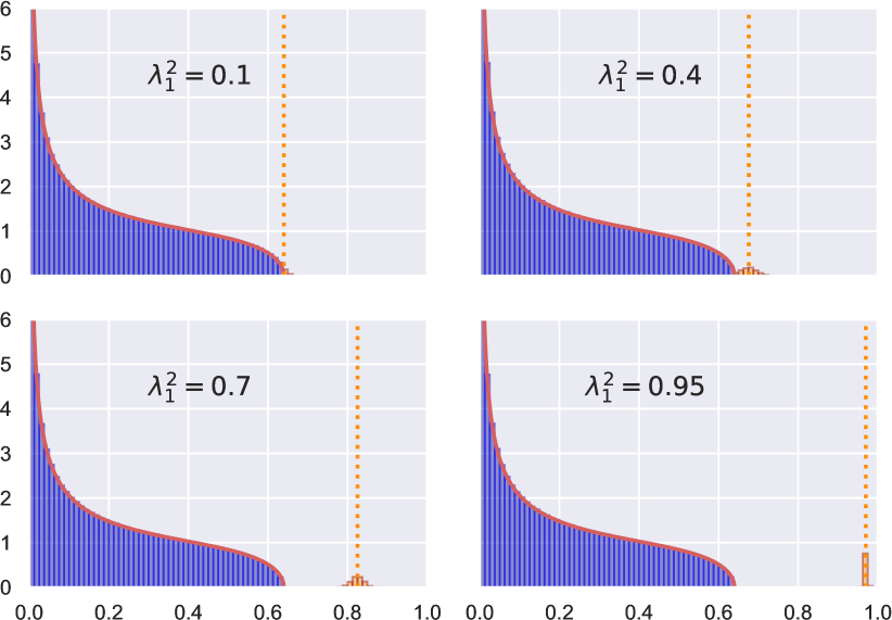
Fig. 5 displays the empirical distribution of the squares of the sample impropriety coefficients under alternative $H_{1}$ spiked model for different spike level $\lambda_{1}$. Again, the bulk of these coefficients matches very well the limiting distribution derived under the properness hypothesis $H_{0}$, whatever the spike level. In addition, for “weak” spikes, i.e. when $\lambda_{1}^{2}$ is small relative to the phase transition threshold $\rho_{c}$ defined in Theorem 9, the greatest sample impropriety coefficient $r_{1}$, which is an estimator of the spike power $\lambda_{1}^{2}$, does not separate from this bulk and is stuck around the edge $c$ of the limiting distribution. Conversely, for stronger spikes where $\lambda_{1}^{2}>\rho_{c}$, $r_{1}$ clearly separates from the bulk and concentrates around the limiting value $\overline{\rho}_{1}$. This numerically supports Theorem 9.

Figure 5: Histogram of the squared sample impropriety coefficients under the spiked impropriety model described in (22) with $N=100$ and $\gamma=5$. Blue bars are for the bulk of the squared impropriety coefficients lower than the edge of the limiting distribution $c$, orange bars are for the ones greater than $c$. The pdf of the limiting distribution under $H_{0}$ given in Theorem 3 is shown in solid red line. The limiting spike values $\overline{\rho}_{1}$ defined in Theorem 9 are depicted as vertical dotted orange lines. The phase transition threshold is here $\rho_{c}=0.25$. Top row sub-figures are for a squared population impropriety coefficient $\lambda_{1}^{2}=0.1<\rho_{c}$ (left) and $\lambda_{1}^{2}=0.4>\rho_{c}$ (right), bottom row is likewise for $\lambda_{1}^{2}=0.7>\rho_{c}$ and $\lambda_{1}^{2}=0.95>\rho_{c}$ respectively. Histograms obtained with $1000$ Monte-Carlo runs.

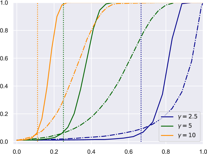
In Fig. 6 the power of both GLRT and Roy’s tests are displayed as a function of the spike power $\lambda_{1}^{2}$. This shows that for “weak” spikes, i.e. when $\lambda_{1}^{2}<\rho_{c}$, the two tests have a very low power. In fact, the largest sample impropriety coefficient $r_{1}$ does not separate from the bulk and cannot be detected correctly using Roy’s test. It is interesting to note that GLRT, which uses the information in all the coefficients, is here slightly “more powerful” to detect such weak spikes. Nevertheless, as soon as $r_{1}$ separates from the bulk, i.e. for stronger spikes where $\lambda_{1}^{2}>\rho_{c}$, Roy’s test becomes much more powerful than the GLRT, with a power that converges quickly towards $1$ as expected.

Figure 6: Power of Roy’s test, solid line, and GLRT, dashdotted line, vs the largest squared population impropriety coefficient $\lambda_{1}^{2}$ under the spiked impropriety model described in (22). The phase transition thresholds $\rho_{c}$ given in Theorem 9 are depicted as vertical dotted lines. Results are shown for different values of $\gamma$: blue lines for $\gamma=2.5$, green for $\gamma=5$, orange for $\gamma=10$ (dimension $N=100$, nominal value of false alarm probability $\alpha=0.01$). Powers estimated with $1000$ Monte-Carlo runs.

IV-B3 Mixed scenario

We consider now a mixed scenario with some highly improper, some less improper, and also some proper components. More precisely, we generate power imbalances between the real and imaginary parts as follows

$$\begin{split}{\bf u}_{m}&={\bf s}_{m},\\ {\bf v}_{m}&={\bf t}_{m}+\sqrt{2\theta}{\bf w}_{m},\end{split}$$ (23)

where $\theta>0$, ${\bf s}_{m}$, ${\bf t}_{m}$ are Gaussian i.i.d. vectors in $\mathbb{R}^{N}$, for $1\leq m\leq M$, and ${\bf w}_{m}$ are i.i.d. Gaussian centered vector where $p_{k}$ denotes, in a principal component analysis, the fraction of variance explained by the $k$th principal component, hence $1\geq p_{1}\geq p_{2}\geq\ldots p_{N}\geq 0$ and $p_{1}+\cdots+p_{n}=1$, and such that ${\bf w}_{m}$ have a unit total variance, i.e. $E\left[||{\bf w}_{m}||_{2}^{2}\right]=1$. Thus the ordered population impropriety coefficients read $\lambda_{k}=\frac{\theta p_{k}}{1+\theta p_{k}}$, for $1\leq k\leq N$.

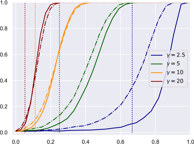
Fig. 7 shows the power of both GLRT and Roy’s test as a function of the principal spike power $\lambda_{1}^{2}$. In this setting, the dimension is $N=20$ and we have that:

• $95\%$ of the variance of the source ${\bf w}_{m}$ is explained by its first five principal components ($p_{1}=50\%$, $p_{2}=20\%$, $p_{3}=p_{4}=10\%$, $p_{5}=5\%$) which yield the most significant (i.e. the largest) impropriety coefficients

• the remaining $5\%$ are explained by the following five components ($p_{6}=\ldots=p_{10}=1\%)$, which yield significantly smaller impropriety coefficients.

As a consequence, half of the impropriety coefficients are non zero, while the other half are zero: $\lambda_{11}=\ldots=\lambda_{20}=0$. This scenario mimics usual principal component analysis where the interesting source lives on a lower dimensional space and its explained variance gradually decreases with the order of the principal components. These curves emphasize that GLRT, which uses all the sample coefficients, can be much more powerful than Roy’s test for small sample size ($\gamma=2.5$ and $\gamma=5$). However for larger values of $\gamma$, Roy’s test becomes significantly more powerful than GLRT for stronger spikes $\lambda_{1}^{2}$. Note also that even if half of the impropriety coefficients are non-zero, the phase transition behavior given in Thm. 9 is still present for Roy’s test.

Figure 7: Power of Roy’s test, solid line, and GLRT, dashdotted line, vs the largest squared population impropriety coefficients $\lambda_{1}^{2}$ under the model described in (23) for dimension $N=20$, with $p_{1}=50\%$, $p_{2}=20\%$, $p_{3}=p_{4}=10\%$, $p_{5}=5\%$, $p_{6}=\ldots=p_{10}=1\%$, and $p_{k}=0$ for $11\leq k\leq 20$. The phase transition thresholds $\rho_{c}$ given in Theorem 9 are depicted as vertical dotted lines. Results are shown for different values of $\gamma$: blue lines for $\gamma=2.5$, green for $\gamma=5$, orange for $\gamma=10$ and red for $\gamma=20$ (nominal value of false alarm probability $\alpha=0.01$). Powers estimated with $1000$ Monte-Carlo runs.

V Relation with existing work on CCA

In CCA, one is classically interested in testing for independence between $N$-dimensional real or complex Gaussian random vectors ${\bf x}$ and ${\bf y}$. Invariant statistics to reject the null hypothesis of independence consist in the squared canonical correlation coefficients. When ${\bf x_{i}}$ and ${\bf y_{i}}$, $1\leq i\leq M$, are $M$ i.i.d. copies of $N$-dimensional real Gaussian independent vectors, the $N$ squared sample canonical correlation coefficients are known to be jointly distributed as the eigenvalues of a matrix-variate beta distribution $\mathcal{B}_{N}(\frac{n_{1}}{2},\frac{n_{2}}{2})$, with $n_{1}=N$ and $n_{2}=M-N$ as shown in [24, Section 11.3].

For the impropriety case, Prop. 2 shows that the $N$ squared impropriety coefficients are jointly distributed as the eigenvalues of a matrix-variate beta distribution $\mathcal{B}_{N}(\tfrac{n_{1}}{2},\tfrac{n_{2}}{2})$ with parameters $n_{1}=N+1$ and $n_{2}=M-N$. Surprisingly, this is quite close to the real and independent CCA case, the difference being a $+1$ offset in the $n_{1}$ parameter. Despite this similarity, it is important to note the following points.

Independence is not compatible with impropriety testing

The two regimes of parameters (in the matrix-variate beta distributions) obtained for the real and independent CCA case or the impropriety case remain incompatible. This is intrinsically due to the fact that the underlying assumptions are not compatible. As shown for instance by (7), the impropriety coefficients are the canonical correlation coefficients between vectors ${\bf z}$ and ${\bf z^{*}}$ which are complex-valued and fully dependent.

Impropriety testing is a more structured problem

Consequently we do not think that classical results for CCA between real, or complex, independent vectors can be readily extended or adapted to the impropriety detection problem. Our contribution is thus a way to overcome this and to provide new insights on the impropriety problem. In this paper we have precisely proposed a direct characterization of the usual impropriety testing statistics. Furthermore, to our knowledge, the numerous existing works on impropriety have never been able to easily adapt these CCA results to characterize impropriety coefficients in finite or even asymptotic regimes.

The $+1$ offset is non-negligible

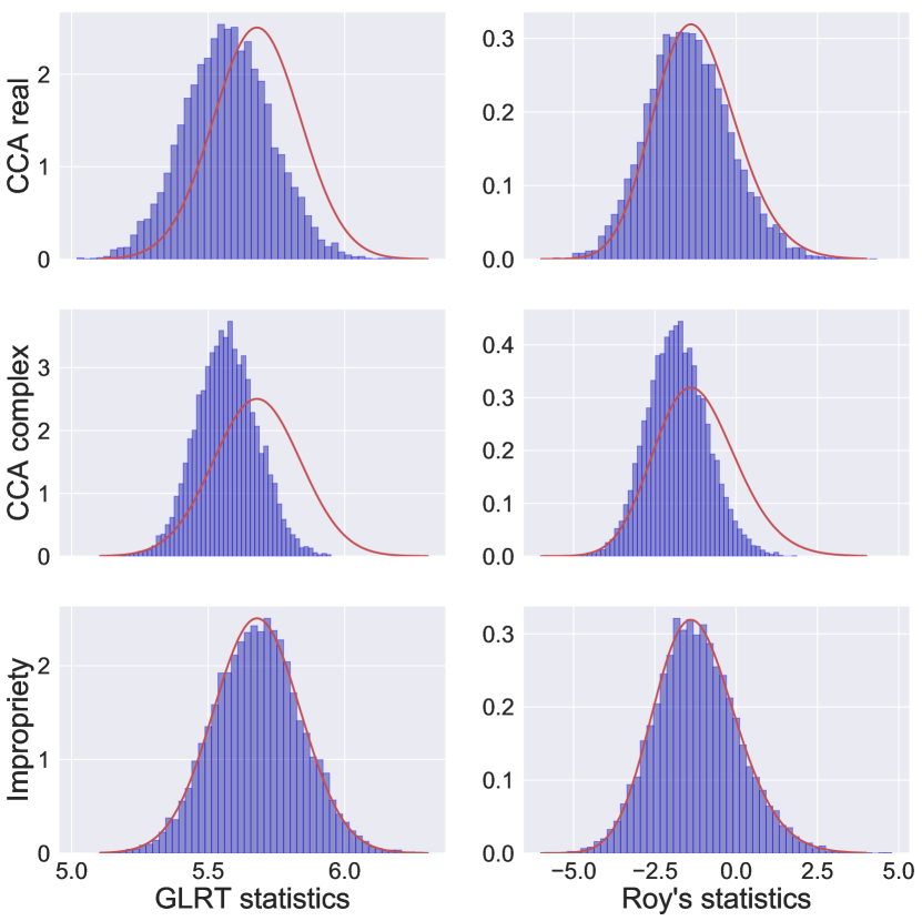
In the high dimensional regime where both $M$ and $N$ go to infinity, it might be tempting to consider that the $+1$ offset in the $n_{1}$ parameter of the matrix-beta distribution becomes negligible, and thus that the distributions of the statistics for testing the independence between real Gaussian vectors or for the impropriety detection problem are asymptotically equivalent. This is actually incorrect. The $+1$ offset modifies the asymptotic distribution of any linear spectral statistic such as the GLRT, but also of the largest eigenvalue one, and therefore of Roy’s test. For instance, Theorem 6 and its demonstration allows us to show that the asymptotic mean $m^{\prime}$ of the GLRT statistics derived for the parameters $n_{1}=N$ and $n_{2}=M-N$ (real and independent CCA case) is $m^{\prime}=m+\ln{\frac{\gamma-1}{\gamma}}$ where $m$ is the asymptotic mean of the impropriety GLRT statistics given in Theorem 6, while the asymptotic variance remains bounded. An illustration of this mismatch for both GLRT and Roy’s test is depicted in Fig. 8.

Figure 8: Histograms for $M=500$ and $N=50$ ($\gamma=10$) of the GLRT statistics (left column) and Roy’s statistics (right column). The pdf of the GLRT and Roy’s test limiting distribution for impropriety testing given in Thm. 6 and Thm. 8 are shown in solid red line in the left and right column respectively. Top row: CCA statistics for independent and real vectors. Middle row: CCA for independent and complex vectors. Bottom row: Impropriety statistics. Histograms obtained with 10000 Monte-Carlo runs.

VI Concluding remarks

Properness testing for complex Gaussian random vectors in the asymptotic regime relies on the characterization of sample impropriety coefficients. In particular, their limiting distributions give access to the behavior of classical GLRT and Roy’s test. The results presented in this article demonstrate that the asymptotic regime is actually reached quite rapidly in practice and the proposed original approximations are well-suited to a wide range of complex-valued datasets.

The phase transition highlighted in Roy’s test has also potential applications in the search for complex-valued low-rank signals corrupted by proper noise in large datasets. In this context, the proposed high dimensional approximations can be extended to the sequential testing problem [31] to estimate the number of improper sources, i.e. of non-zero impropriety coefficients. Another natural extension of the proposed work consists of considering the case of quaternion random vectors which possess several properness levels, thus trying to decipher their correlation symmetry patterns. This could be helpful in the spectral characterization of bivariate signals [32] among other quaternion signal processing applications.

Appendix A Proof of Theorem 3 (limiting empirical distribution)

According to Proposition 2, the sample squared impropriety coefficients are distributed under $H_{0}$ as the eigenvalues of a matrix-variate Beta distribution $\mathcal{B}_{N}(\frac{1}{2}n_{1},\frac{1}{2}n_{2})$. Moreover, [24, Thm 3.3.1, p. 109] shows that the eigenvalues of a $\mathcal{B}_{N}(\frac{1}{2}n_{1},\frac{1}{2}n_{2})$ random matrix are distributed as the eigenvalues of ${\bf A}({\bf A}+{\bf B})^{-1}$, where ${\bf A},{\bf B}\in{\mathbb{R}}^{N\times N}$ are two independent random matrices with respective distributions the Wishart laws $W_{N}(n_{1},{\bf I}_{N})$ and $W_{N}(n_{2},{\bf I}_{N})$, where $n_{1}$ and $n_{2}$ are their respective number of degrees of freedom and where the Wishart scaling matrix parameter is set to the identity matrix ${\bf I}_{N}$. Thus the limiting distribution for the impropriety coefficients can be derived as the limiting distribution of the eigenvalues of ${\bf A}({\bf A}+{\bf B})^{-1}$.

Assume now that we are in the asymptotic regime where $N,n_{1},n_{2}\,\rightarrow\,+\infty$ with $N/n_{1}\,\rightarrow\,d\in(0,1]$ and $N/n_{2}\,\rightarrow\,d^{\prime}\in(0,1)$.

Then, as demonstrated in [33], the empirical law of the eigenvalues of the following $F$-matrix $\tfrac{d}{d^{\prime}}{\bf A}{\bf B}^{-1}$ converges to a distribution with density given as:

$$f(x)=\frac{(1-d^{\prime})\sqrt{(x-a)(b-x)}}{2\pi x(xd+d^{\prime})},$$ (24)

on the interval $x\in[a,b]$, where $a=\left(\tfrac{1-\sqrt{1-(1-d)(1-d^{\prime})}}{1-d^{\prime}}\right)^{2}$ and $b=\left(\tfrac{1+\sqrt{1-(1-d)(1-d^{\prime})}}{1-d^{\prime}}\right)^{2}$.

Note that each eigenvalue $r_{i}$ of ${\bf A}({\bf A}+{\bf B})^{-1}$ can be deduced from each eigenvalue $x_{i}$ of $\tfrac{d}{d^{\prime}}{\bf A}{\bf B}^{-1}$ thanks to the relation $r_{i}=\tfrac{d^{\prime}x_{i}}{d+d^{\prime}x_{i}}$. The continuous mapping theorem ensures therefore that the asymptotic law of the eigenvalues of a $\mathcal{B}_{N}(\frac{1}{2}n_{1},\frac{1}{2}n_{2})$ random matrix can be directly deduced from (24) using the aforementioned change of variable.

Last, according to proposition 2, the parameters for the matrix-variate Beta distribution in our case are $n_{1}=N+1$ and $n_{2}=M-N$. Due to the asymptotic regime stated above, one gets that $d=\lim\,N/n_{1}=1$ and $d^{\prime}=\lim\,N/n_{2}=\tfrac{1}{\gamma-1}$. Plugging this parameter values in the asymptotic distribution of the eigenvalues of the $\mathcal{B}_{N}(\frac{1}{2}n_{1},\frac{1}{2}n_{2})$ random matrix deduced from (24) gives finally the limiting density given in Theorem 3 and concludes the proof.

Appendix B Proof of Theorem 6 (central limit theorem)

According to theorem 5, $T^{\prime}=\sum_{n=1}^{N}\zeta_{n}$ where the $\zeta_{n}$ are independent random variables such that $\zeta_{n}=-\ln u_{n}$ with $u_{n}$ beta distributed s.t. $u_{n}\sim\mathcal{B}\left(a_{n},b\right)$, $a_{n}=\tfrac{M-N-n+1}{2}$, $b=\tfrac{N+1}{2}$, for $1\leq n\leq N$. Based on the centered moments of a logarithmically transformed beta-distributed variable as given in [34], then $E[\zeta_{n}]=\psi(a_{n}+b)-\psi(a_{n})$ where $\psi(\cdot)$ is the digamma function, and $\operatorname{var}[\zeta_{n}]=\psi_{1}(a_{n})-\psi_{1}(a_{n}+b)$ where $\psi_{1}(\cdot)$ is the trigamma function. Using asymptotic expansions of the digamma and trigamma functions for large argument $x$,

$$\psi(x) =\log{x}-\tfrac{1}{2x}+O\left(\tfrac{1}{x^{2}}\right),\quad\psi_{1}(x)=\tfrac{1}{x}+\tfrac{1}{2x^{2}}+O\left(\tfrac{1}{x^{3}}\right),$$

plus Stirling formula $\log{(n!)}=n\log{n}-n+\tfrac{1}{2}\log{(2\pi n)}+O\left(\tfrac{1}{n}\right)$ for large $n$, straightforward computations omitted here for the sake of brevity yield that $E[T^{\prime}]=\sum_{n=1}^{N}E[\zeta_{n}]=m_{M}+O(1/M)$ and $\operatorname{var}(T^{\prime})=\sum_{n=1}^{N}\operatorname{var}(\zeta_{n})=s_{M}^{2}+O(1/M^{2})$.

In order to apply Lyapunov central limit theorem [35, p. 362] to ${T^{\prime}=\sum_{n=1}^{N}\zeta_{n}}$, it is sufficient to show that

$$\frac{1}{\operatorname{var}(T^{\prime})^{2}}\sum_{n=1}^{N}E\left[\left(\zeta_{n}-E[\zeta_{n}]\right)^{4}\right]\,\rightarrow\,0.$$

The expression of the fourth order centered moment of $\zeta_{n}$ gives that $E\left[\left(\zeta_{n}-E[\zeta_{n}]\right)^{4}\right]=O\left(1/(M-n+2)^{2}\right)$ for $1\leq n\leq N$. Then $\sum_{n=1}^{N}E\left[\left(\zeta_{n}-E[\zeta_{n}]\right)^{4}\right]=O(1/M)$. As $\operatorname{var}(T^{\prime})=s_{M}^{2}+O(1/M^{2})$, it comes that $\operatorname{var}(T^{\prime})^{-2}=O(1)$ and the previous Lyapunov sufficient condition holds. Thus

$$Z\equiv\frac{1}{\sqrt{\operatorname{var}(T^{\prime})}}\sum_{n=1}^{N}\left(\zeta_{n}-E[\zeta_{n}]\right)\ {\xrightarrow{d}}\ \mathcal{N}(0,1).$$

By noting finally that $\frac{1}{s_{M}}(T^{\prime}-m_{M})=Z+O(1/M)$, Slutsky’s theorem allows us to conclude the proof.

References

- [1] P. Comon, “Circularité et signaux aléatoires à temps discret,” Traitement du Signal, vol. 11, pp. 41–420, 1994.
- [2] B. Picinbono, “On circularity,” IEEE Trans. on Signal Processing, vol. 42, no. 12, pp. 3473–3482, 1994.
- [3] E. Ollila and V. Koivunen, “Generalized complex elliptical distributions,” in IEEE Sensor Array and Multichannel Signal Processing workshop (SAM), 2004, pp. 460–464.
- [4] P. Schreier, L. Scharf, and A. Hanssen, “A generalized likelihood ratio test for impropriety of complex signals,” IEEE Signal Processing Letters, vol. 13, no. 7, pp. 433 – 436, 2006.
- [5] P. Schreier and L. Scharf, Statistical Signal Processing of Complex-Valued Data: The Theory of Improper and Noncircular Signals. Cambridge University Press, 2010.
- [6] S. Chandna and A. Walden, “A frequency domain test for propriety of complex-valued vector time series,” IEEE Transactions on Signal Processing, vol. 65, pp. 1425–1436, 2017.
- [7] J. Delmas, A. Oukaci, and P. Chevalier, “On the asymptotic distribution of glr for impropriety of complex signals,” Signal Processing, vol. 91, no. 10, pp. 2259–2267, 2011.
- [8] A. Walden and P. Rubin-Delanchy, “On testing for impropriety of complex-valued gaussian vectors,” IEEE Transactions on Signal Processing, vol. 57, no. 3, pp. 21–51, 2009.
- [9] F. Chatelain and N. Le Bihan, “Exact distribution and high-dimensional asymptotics for improperness test of complex signals,” in ICASSP 2019 - 2019 IEEE International Conference on Acoustics, Speech and Signal Processing (ICASSP), May 2019, pp. 8509–8513.
- [10] S. Zarei, W. H. Gerstacker, J. Aulin, and R. Schober, “I/Q imbalance aware widely-linear receiver for uplink multi-cell massive mimo systems: Design and sum rate analysis,” IEEE Transactions on Wireless Communications, vol. 15, no. 5, pp. 3393–3408, May 2016.
- [11] E. Axell, G. Leus, E. G. Larsson, and H. V. Poor, “Spectrum sensing for cognitive radio : State-of-the-art and recent advances,” IEEE Signal Processing Magazine, vol. 29, no. 3, pp. 101–116, May 2012.
- [12] T. Adali, P. J. Schreier, and L. L. Scharf, “Complex-valued signal processing: The proper way to deal with impropriety,” IEEE Transactions on Signal Processing, vol. 59, no. 11, pp. 5101–5125, Nov 2011.
- [13] J. Dong, F. Krzakala, and S. Gigan, “Spectral method for multiplexed phase retrieval and application in optical imaging in complex media,” in ICASSP 2019 - 2019 IEEE International Conference on Acoustics, Speech and Signal Processing (ICASSP), May 2019, pp. 4963–4967.
- [14] S. Andersson and M. Perlman, “Two testing problems relating the real and complex multivariate normal distributions,” Journal of Multivariate Analysis, vol. 15, pp. 21–51, 1975.
- [15] C. Hellings and W. Utschick, “Measuring impropriety in complex and real representations,” Signal Processing, vol. 164, pp. 267–283, 11 2019.
- [16] N. Klausner, M. R. Azimi-Sadjadi, and L. L. Scharf, “Detection of spatially correlated time series from a network of sensor arrays,” IEEE Transactions on Signal Processing, vol. 62, no. 6, pp. 1396–1407, March 2014.
- [17] I. Santamaria, L. L. Scharf, J. Via, Y. Wang, and H. Wang, “Passive detection of correlated subspace signals in two mimo channels,” IEEE Trans. Signal Processing, vol. 65, no. 20, pp. 5266–5280, October 2017.
- [18] X. Mestre, P. Vallet, and W. Hachem, “Correlation test for high dimensional data with application to signal detection in sensor networks,” in 2014 22nd European Signal Processing Conference (EUSIPCO), Sep. 2014, pp. 2165–2169.
- [19] T. Adali and V. D. Calhoun, “Complex ICA of brain imaging data [life sciences],” IEEE Signal Processing Magazine, vol. 24, no. 5, pp. 136–139, 2007.
- [20] J.-P. Delmas, “Asymptotically minimum variance second-order estimation for noncircular signals with application to doa estimation,” IEEE Transactions on Signal Processing, vol. 52, no. 5, pp. 1235–1241, 2004.
- [21] E. L. Lehmann and J. P. Romano, Testing statistical hypotheses, 3rd ed., ser. Springer Texts in Statistics. New York: Springer, 2005.
- [22] J. Eriksson and V. Koivunen, “Complex random vectors and ICA models: identifiability, uniqueness, and separability,” IEEE Transactions on Information Theory, vol. 52, no. 3, pp. 1017–1029, 2006.
- [23] E. Moreau and T. Adali, Blind Identification and Separation of Complex-Valued Signals. ISTE-Wiley, 2013.
- [24] R. Muirhead, Aspects of Multivariate Statistical Theory. Wiley-Interscience, 2005.
- [25] K. V. Mardia, J. T. Kent, and J. M. Bibby, Multivariate analysis. Academic Press London ; New York, 1979.
- [26] T. Hasija, C. Lameiro, and P. J. Schreier, “Determining the dimension of the improper signal subspace in complex-valued data,” IEEE Signal Processing Letters, vol. 24, no. 11, pp. 1606–1610, Nov 2017.
- [27] I. Johnstone, “Approximate null distribution of the largest root in multivariate analysis,” Ann. Appl. Stat., vol. 3, pp. 1616–1633, 2009.
- [28] M. Chiani, “Distribution of the largest root of a matrix for roy’s test in multivariate analysis of variance,” J. Multivar. Anal., vol. 143, pp. 467–471, 2016.
- [29] Z. Bao, J. Hu, G. Pan, and W. Zhou, “Canonical correlation coefficients of high-dimensional gaussian vectors: Finite rank case,” Ann. Statist., vol. 47, no. 1, pp. 612–640, 02 2019. [Online]. Available: https://doi.org/10.1214/18-AOS1704
- [30] I. Johnstone and A. Onatski, “Testing in high-dimensional spiked models,” arXiv e-prints, p. arXiv:1509.07269v2, Feb 2018.
- [31] M. Novey, E. Ollila, and T. Adali, “On testing the extent of noncircularity,” IEEE Transactions on Signal Processing, vol. 59, no. 11, pp. 5632–5637, 2011.
- [32] J. Flamant, N. Le Bihan, and P. Chainais, “Spectral analysis of stationary random bivariate signals,” IEEE Transactions on Signal Processing, vol. 65, no. 23, pp. 6135–6145, Dec 2017.
- [33] J. Silverstein, “The limiting eigenvalue distribution of a multivariate F matrix,” SIAM J. Math. Anal., vol. 16, pp. 641–646, 1985.
- [34] S. Nadarajah and S. Kotz, “The beta exponential distribution,” Reliability Engineering & System Safety, vol. 91, no. 6, pp. 689 – 697, 2006.
- [35] P. Billingsley, Probability and Measure, ser. Wiley Series in Probability and Statistics. Wiley, 1995.