Supersolid phase of the extended Bose-Hubbard model with an artificial gauge field

Abstract

We examine the zero and finite temperature phase diagrams of soft-core bosons of the extended Bose-Hubbard model on a square optical lattice. To study various quantum phases and their transitions we employ single-site and cluster Gutzwiller mean-field theory. We have observed that the Mott insulator phase vanishes above a critical value of nearest-neighbour interaction and the supersolid phase occupies a larger region in the phase diagram. We show that the presence of artificial gauge field enlarges the domain of supersolid phase. The finite temperature destroys the crystalline structure of the supersolid phase and thereby favours normal fluid to superfluid phase transition. The presence of an envelope harmonic potential demonstrates coexistence of different phases and at $z~{}k_{B}T\geqslant V$, thermal energy comparable and higher to the long-range interaction energy, the supersolidity of the system is destroyed.

I Introduction

Ultracold atomic systems have played an important role in the study of quantum many-body systems. In particular, the novel experimental developments in manipulating ultracold atoms in optical lattices have led to the realization of new quantum states and quantum phase transitions in strongly correlated systems Lewenstein et al. (2007); Bloch et al. (2008). In recent years, there has been a surge of interest in understanding the supersolid (SS) phase which is characterized by the simultaneous appearance of a crystalline and an off-diagonal long-range orders Leggett (1970); Chester (1970). This phase breaks two continuous symmetries: the phase invariance of the superfluid (SF) and translational invariance to form crystal. Although the SS phase was predicted in liquid ⁴He a long time ago Andreev and Lifshitz (1969); Thouless (1969), the experimental observation of supersolidity in liquid ⁴He remains elusive Kim and Chan (2004a, b, 2012). However, the quest for SS phase has gained new impetus following the remarkable theoretical insights and experimental achievements in ultracold atoms in optical lattices, which are excellent quantum many-body systems to observe SS phase as these are clean and controllable. Recently, the characteristic signature of SS phase has been observed in ultracold atoms Léonard et al. (2017); Li et al. (2017); Tanzi et al. (2019a); Böttcher et al. (2019); Chomaz et al. (2019) and this phase may emerge by tuning the bosonic interactions of different length scales Landig et al. (2016). Furthermore, the excitation spectrum and various properties of SS phase have been observed in recent quantum gas experiments Natale et al. (2019); Tanzi et al. (2019b); Guo et al. (2019).

On the theoretical aspects, the existence of SS phase has been studied using the extended Bose-Hubbard model (eBHM). The checkerboard supersolid phase of hard-core bosons is thermodynamically unstable towards phase separation and this phase is not stabilized by next NN (NNN) interaction Batrouni and Scalettar (2000). However, in the soft-core model, due to larger Fock-space and possibility of higher number fluctuations, the SS order is stable with NN interaction van Otterlo et al. (1995); Sengupta et al. (2005); Ohgoe et al. (2012a). Similarly, SS phase emerges in the honeycomb lattices when the hard-core limit of bosons is relaxed Wessel (2007); Gan et al. (2007). The existence and stability of supersolidity have also been confirmed for bosons with infinite-range cavity-mediated interactions Flottat et al. (2017). The SS phase has been explored in various lattice systems, such as one-dimensional (1D) chain Mathey et al. (2009); Batrouni et al. (2006) and ladder Sachdeva et al. (2017), two-dimensional (2D) square Góral et al. (2002); Sengupta et al. (2005); Scarola and Das Sarma (2005); Yi et al. (2007); Ng and Chen (2008); Capogrosso-Sansone et al. (2010); Bandyopadhyay et al. (2019), triangular Wessel and Troyer (2005); Heidarian and Damle (2005); Melko et al. (2005); Boninsegni and Prokof’ev (2005); Sen et al. (2008); Yamamoto et al. (2012a), honeycomb Wessel (2007); Gan et al. (2007), kagome Isakov et al. (2006); Huerga et al. (2016), bilayer lattice of dipolar bosons Trefzger et al. (2009), and three-dimensional (3D) cubic lattice Yi et al. (2007); Yamamoto et al. (2009); Xi et al. (2011); Ohgoe et al. (2012b). The eBHM with artificial gauge field has been studied to examine the fractional quantum Hall Kuno et al. (2017) and vortex-solid states Kuno et al. (2015).

In this work we investigate theoretically the presence of SS phase of soft-core bosons in 2D square optical lattice with long-range interaction and artificial gauge field. The long-range interaction can be realized with the dipolar ultracold atoms Pasquiou et al. (2011); Baier et al. (2016). And, it is possible to introduce artificial gauge field with lasers Aidelsburger et al. (2011); Miyake et al. (2013); Atala et al. (2014); Kennedy et al. (2015). For our studies we use the single-site and cluster mean-field theories. We show that the combined effect of the long-range interaction and artificial gauge field increases the domain of the SS phase. In particular, we examine the effect of magnetic flux quanta on the SS-SF phase boundary in the presence of the NN interaction. Furthermore, to relate with experimental realizations, we incorporate the effects of thermal fluctuations arising from finite temperatures.

The paper is organized as follows. In Sec. II we introduce the model considered in our study and describe theoretical approach employed. Here we provide description of the single-site, cluster and finite temperature Gutzwiller (GW) mean-field theories. The ground-state phase diagrams and study of dipolar atoms in the confining potential are presented in Sec. III. Finally, we conclude with the key findings of the present work in Sec. IV.

II Theoretical Methods

II.1 Extended Bose-Hubbard model

Consider a system of bosonic atoms with long-range interactions in a 2D square optical lattice in the presence of synthetic magnetic field. The temperature of the system is low such that all the atoms occupy the lowest Bloch band. Such a system is well described by eBHM, and the Hamiltonian of the model is

$$\hat{H}_{\rm eBHM} = -\sum_{p,q}\left(J_{x}\hat{b}^{\dagger}_{p+1,q}\hat{b}_{p,q}+J_{y}\hat{b}^{\dagger}_{p,q+1}\hat{b}_{p,q}+\rm{H.c.}\right)$$ (1)

$$+\sum_{p,q}\hat{n}_{p,q}\left[\left(\epsilon_{p,q}-\mu\right)+\frac{U}{2}(\hat{n}_{p,q}-1)\right]$$

$$+\sum_{\langle\xi\xi^{\prime}\rangle}V_{\xi,\xi^{\prime}}~{}\hat{n}_{\xi}\hat{n}_{\xi^{\prime}},$$

where $p(q)$ is the lattice site index along $x(y)$ direction, $\hat{b}^{\dagger}_{p,q}$ ($\hat{b}_{p,q}$) is the bosonic operator which creates (annihilates) an atom at the lattice site $(p,q)$, $\hat{n}_{p,q}=\hat{b}^{\dagger}_{p,q}\hat{b}_{p,q}$ is the boson number operator, $J_{x}$ and $J_{y}$ are the tunneling or hopping strength between two NN sites along $x$ and $y$ directions, respectively, $\epsilon_{p,q}$ is the offset energy arising due to the presence of external envelope potential, $\mu$ is the chemical potential, and $U>0$ is the on-site interatomic interaction. Here $\xi$ is a combination of lattice indices in 2D, that is, $\xi\equiv(p,q)$ and $\xi^{\prime}\equiv(p^{\prime},q^{\prime})$ are neighbouring sites to $\xi$. The long-range interaction $V_{\xi,\xi^{\prime}}$ is given by

$$V_{\xi,\xi^{\prime}}=\begin{cases}V_{1}&\text{ if $|\mathbf{r}_{pq}-\mathbf{r}_{p^{\prime}q^{\prime}}|=a$},\\ V_{2}&\text{ if $|\mathbf{r}_{pq}-\mathbf{r}_{p^{\prime}q^{\prime}}|=\sqrt{2}a$},\\ 0&\text{ otherwise},\end{cases}$$ (2)

where $a$ is the lattice spacing, ${\bf r}_{pq}=(pa,qa)$ is the lattice site coordinates. The parameters $V_{1}\geqslant 0$ and $V_{2}\geqslant 0$ are the NN and NNN interactions, respectively. In the present work, we consider $V_{2}/V_{1}=1/2\sqrt{2}$ which corresponds to inverse cube power law of isotropic dipolar interaction. These terms encapsulate the observable effects of the dipolar interaction in the system. The higher $V_{1}$ as compared to $V_{2}$ tends to induce checkerboard density pattern for density wave (DW) and SS phases. This minimal model captures the essential physics arising due to the hopping induced competition among different solid orders and the superfluidity. We also consider this model to examine the ground states of inhomogeneous dipolar bosons at zero and finite temperatures in optical lattices with an envelope confining harmonic potential.

II.2 Artificial gauge field

The long-range interaction in the above Hamiltonian, Eq. (1), is characteristic or inherent to the internal state of the atomic species. In terms of the many-body physics, the nature of the correlation can further be modified through the introduction of artificial gauge field. The presence of the artificial gauge field modifies the Hamiltonian to

$$\hat{H}_{\rm eBHM} = -\sum_{p,q}\left(J_{x}e^{i2\pi\alpha q}\hat{b}^{\dagger}_{p+1,q}\hat{b}_{p,q}+J_{y}\hat{b}^{\dagger}_{p,q+1}\hat{b}_{p,q}+\rm{H.c.}\right)$$ (3)

$$+\sum_{p,q}\hat{n}_{p,q}\left[\left(\epsilon_{p,q}-\mu\right)+\frac{U}{2}(\hat{n}_{p,q}-1)\right]$$

$$+\sum_{\langle\xi\xi^{\prime}\rangle}V_{\xi,\xi^{\prime}}~{}\hat{n}_{\xi}\hat{n}_{\xi^{\prime}},$$

where the strength of the magnetic field is reflected in the number of flux quanta per plaquette $\alpha=(e/\hbar)\int d{\mathbf{r}}.\mathbf{A(r)}$. Here, $0\leqslant\alpha<1$, and $\mathbf{A(r)}$ is the vector potential which gives rise to synthetic magnetic field $\mathbf{B=\nabla\times A}$. In the presence of the synthetic magnetic field, atoms acquire a $2\pi\alpha$ phase when they hop around a plaquette. This results into a phase shift in the hopping strength of the model. Physically, the synthetic magnetic field introduces a force on the atoms which is equivalent of the Lorentz force on a charged particle in the presence of external magnetic field. The system is then a charge neutral analogue of the quantum Hall system in condensed matter systems. For the present study, we consider Landau gauge, where the vector potential $\mathbf{A(r)}=-By\hat{x}$. Hence, for the homogeneous system, at zero magnetic field the system possesses the translational invariance along both axes, whereas in the presence of magnetic field the system preserves the invariance only along the $x$-axis of the lattice.

II.3 Gutzwiller mean-field theory

To study the ground-states of the systems described by the model Hamiltonians in Eq. (1) and (3) and their properties we use single-site Gutzwiller mean-field (SGMF) and cluster Gutzwiller mean-field (CGMF) theories. The later is the extension of SGMF which incorporates the correlation within a cluster of neighbouring sites exactly. In the SGMF theory Rokhsar and Kotliar (1991); Krauth et al. (1992); Sheshadri et al. (1993); Bai et al. (2018); Pal et al. (2019); Bandyopadhyay et al. (2019), the bosonic operators are expanded about their expectation values as

$$\hat{b}_{p,q}=\phi_{p,q}+\delta\hat{b}_{p,q},$$ (4a)

$$\hat{b}^{\dagger}_{p,q}=\phi^{*}_{p,q}+\delta\hat{b}^{\dagger}_{p,q}.$$ (4b)

Therefore, the product of the creation and annihilation operators which occurs in the hopping term can be written as

$$\hat{b}^{\dagger}_{p,q}\hat{b}_{p^{\prime},q^{\prime}}\approx\phi^{*}_{p,q}\hat{b}_{p^{\prime},q^{\prime}}+\hat{b}^{\dagger}_{p,q}\phi_{p^{\prime},q^{\prime}}-\phi^{*}_{p,q}\phi_{p^{\prime},q^{\prime}},$$ (5)

where second order terms in the fluctuation $\delta\hat{b}_{p,q}$ are neglected. Here, $\phi_{p,q}=\langle\hat{b}_{p,q}\rangle$ is the SF order parameter of the system. Using above approximation in the Hamiltonian, Eq. (3), the single-site mean-field Hamiltonian is

$$\hat{H}^{\rm MF}_{p,q} = -\bigg{[}J_{x}e^{i2\pi\alpha q}\left(\phi^{*}_{p+1,q}\hat{b}_{p,q}-\phi^{*}_{p+1,q}\phi_{p,q}\right)$$ (6)

$$+J_{y}\left(\phi^{*}_{p,q+1}\hat{b}_{p,q}-\phi^{*}_{p,q+1}\phi_{p,q}\right)+\rm{H.c.}\bigg{]}$$

$$+\left[(\epsilon_{p,q}-\mu)+\frac{U}{2}(\hat{n}_{p,q}-1)\right]\hat{n}_{p,q}$$

$$+\sum_{\langle\xi,\xi^{\prime}\rangle}V_{\xi,\xi^{\prime}}~{}\left(\hat{n}_{\xi}\langle\hat{n}_{\xi^{\prime}}\rangle-\langle\hat{n}_{\xi}\rangle\langle\hat{n}_{\xi^{\prime}}\rangle\right)$$

and the total Hamiltonian of the system is

$$\hat{H}_{\rm MF}=\sum_{p,q}\hat{H}^{\rm MF}_{p,q}.$$ (7)

Here, the neighbouring lattice sites are coupled through $\phi_{p,q}$, the SF order parameter. And therefore the eigenstate of the entire lattice is the product of single-site states. Accordingly, the many-body wave function of the ground state of the system is given by the Gutzwiller ansatz

$$\ket{\Psi}=\prod_{p,q}\ket{\psi}_{p,q}=\prod_{p,q}\left(\sum^{N_{b}}_{n=0}c^{(p,q)}_{n}\ket{n}_{p,q}\right),$$ (8)

where $\ket{\psi}_{p,q}$ is the single-site ground state, $N_{b}$ is the number of occupation basis or maximum number of bosons at each lattice site, $\ket{n}_{p,q}$ is the occupation or Fock state of $n$ bosons occupying the site $(p,q)$ and $c^{(p,q)}_{n}$ are the coefficients of the occupation state. The normalization of the wave function leads to the normalization of $c^{(p,q)}_{n}$ at each lattice site as $\Sigma_{n}|c^{(p,q)}_{n}|^{2}=1$. Using the above ansatz the SF order parameter $\phi_{p,q}=\bra{\Psi}\hat{b}_{p,q}\ket{\Psi}$ is obtained as

$$\phi_{p,q}=\sum^{N_{b}}_{n=0}\sqrt{n}~{}c^{(p,q)*}_{n-1}c^{(p,q)}_{n}.$$ (9)

Similarly, the occupancy of each lattice site $n_{p,q}=\bra{\Psi}\hat{b}^{\dagger}_{p,q}\hat{b}_{p,q}\ket{\Psi}$ is

$$n_{p,q}=\sum^{N_{b}}_{n=0}n|c^{(p,q)}_{n}|^{2}.$$ (10)

The two parameters $\phi_{p,q}$ and $n_{p,q}$, together serve to define the quantum phases of the system. Using the mean-field Hamiltonian, Eq. (6), the total energy of the system $E=\bra{\Psi}\hat{H}_{\rm MF}\ket{\Psi}$ is obtained as a sum of the single-site energies $E_{p,q}=\bra{\Psi}\hat{H}_{p,q}^{\rm MF}\ket{\Psi}$. And, $E$ is minimized self consistently with the Eqs. (9) and (10) to obtain the ground state of the system.

In the CGMF theory, a lattice of dimension $K\times L$ is partitioned into $W$ clusters of size $M\times N$, that is $W=(K\times L)/(M\times N)$  Buonsante et al. (2004); Yamamoto (2009); Pisarski et al. (2011); McIntosh et al. (2012); Lühmann (2013); Bai et al. (2018); Pal et al. (2019). Then, the hopping terms of the model are decomposed into two types. One is the exact term which corresponds to hopping within the cluster, and the other is the inter-cluster hopping between lattice sites which lie on the boundary of two neighbouring clusters. The latter is defined by coupling through the mean-field or the SF order parameter. The Hamiltonian of a cluster is

$$\hat{H}_{C} = -{\sum_{p,q\in C}}^{\prime}\left(J_{x}e^{i2\pi\alpha q}\hat{b}_{p+1,q}^{\dagger}\hat{b}_{p,q}+J_{y}\hat{b}_{p,q+1}^{\dagger}\hat{b}_{p,q}+{\rm H.c.}\right)$$ (11)

$$-\sum_{p,q\in\delta C}\left(J_{x}{\rm e}^{i2\pi\alpha q}(\phi^{c}_{p+1,q})^{\ast}\hat{b}_{p,q}+J_{y}(\phi^{c}_{p,q+1})^{\ast}\hat{b}_{p,q}+{\rm H.c.}\right)$$

$$+\sum_{p,q\in C}\left[(\epsilon_{p,q}-\mu)\hat{n}_{p,q}+\frac{U}{2}\hat{n}_{p,q}(\hat{n}_{p,q}-1)\right]$$

$$+\sum_{\langle\xi\xi^{\prime}\rangle\in C}V_{\xi,\xi^{\prime}}~{}\hat{n}_{\xi}~{}\hat{n}_{\xi^{\prime}}+\sum_{\langle\xi\xi^{\prime}\rangle\in\delta C}V_{\xi,\xi^{\prime}}~{}\hat{n}_{\xi}~{}\langle\hat{n}_{\xi^{\prime}}\rangle,$$

where the model parameters $J_{x}$, $J_{y}$, $U$ and $V_{\xi,\xi^{\prime}}$ are defined as in SGMF and prime in the first summation indicates that the $(p+1,q)$ and $(p,q+1)$ lattice sites are also within the cluster. Here, $\delta C$ in the second summation represents the lattice sites at the boundary of the clusters and $(\phi^{c}_{p,q})=\sum_{p^{\prime},q^{\prime}\not\in C}\langle\hat{b}_{p^{\prime},q^{\prime}}\rangle$ is the SF order parameter at the lattice site which lies at the boundary of neighbouring cluster. As hopping parameter, the long-range interaction term also has two contributions, one is within the cluster which is exact, and the other is inter-cluster interaction at the boundary which is defined through the mean occupancy $\langle\hat{n}_{\xi^{\prime}}\rangle$. The matrix elements of $\hat{H}_{C}$ are, then, calculated in terms of the cluster basis states

$$\ket{\Phi_{c}}_{\ell}=\prod_{q=0}^{N-1}\prod_{p=0}^{M-1}\ket{n_{p}^{q}},$$ (12)

where $\ket{n_{p}^{q}}$ is the occupation number basis at the $(p,q)$ lattice site, and $\ell\equiv\{n_{0}^{0},n_{1}^{0},\ldots,n_{M-1}^{0},n_{0}^{1},n_{1}^{1},\ldots n_{M-1}^{1},\ldots,n_{M-1}^{N-1}\}$ is the index quantum number to identify the cluster state. After diagonalizing the Hamiltonian, we can get the ground state of the cluster as

$$|\Psi_{c}\rangle=\sum_{\ell}C_{\ell}\ket{\Phi_{c}}_{\ell},$$ (13)

where $C_{\ell}$ are components of the eigenvector, and naturally satisfy the normalization condition $\sum_{\ell}|C_{\ell}|^{2}=1$. The ground state of the entire $K\times L$ lattice, as in SGMF, is the direct product of the cluster ground states

$$\ket{\Psi^{c}_{\rm GW}}=\prod_{k}\ket{\Psi_{c}}_{k},$$ (14)

where $k$ is the cluster index and varies from 1 to $W=(K\times L)/(M\times N)$. The SF order parameter $\phi$, as in Eq. (9), can be computed in terms of the cluster states. The average occupancy of the $k$th cluster can also be computed similarly.

II.4 Finite temperature Gutzwiller mean-field theory

At finite temperature, the thermal fluctuations modify the properties of the system, and observable properties are the thermal averages. To calculate the thermal averages we need the entire eigenspectrum. So, in the SGMF, we retain the entire energy spectrum $E^{l}_{p,q}$ and the eigenstates $\ket{\psi}^{l}_{p,q}$ obtained from the diagonalization of the single-site Hamiltonian $\hat{H}^{\rm MF}_{p,q}$ in Eq. (6). Then, we evaluate the single-site partition function of the system

$$Z=\sum_{l=1}^{N_{b}}e^{-\beta E^{l}},$$ (15)

where $\beta=1/k_{B}T$ and $T$ is the temperature of the system. At finite $T$, the region in the phase diagram with $\phi=0$ and the real occupancy $\langle\hat{n}_{p,q}\rangle$ is identified as the normal fluid (NF) phase. Similarly, in the CGMF, the partition function is defined in terms of all the eigenvalues $E^{l}_{k}$ and eigenfunctions $\ket{\Psi_{c}}^{l}_{k}$ of each $k$th cluster from all the $W$ clusters.

From the definition of the partition function, in the SGMF, the thermal average of $\phi_{p,q}$ is

$$\langle\phi_{p,q}\rangle=\frac{1}{Z}\sum_{i=0}^{N_{b}}\prescript{i}{p,q}{\bra{\psi}}\hat{b}_{p,q}e^{-\beta E^{i}}\ket{\psi}^{i}_{p,q},$$ (16)

where $\langle\ldots\rangle$ represents the thermal averaging. Similarly, the occupancy or the density at finite $T$ is defined as

$$\langle\langle\hat{n}_{p,q}\rangle\rangle=\frac{1}{Z}\sum_{i=0}^{N_{b}}\prescript{i}{p,q}{\bra{\psi}}\hat{n}_{p,q}e^{-\beta E^{i}}\ket{\psi}^{i}_{p,q}.$$ (17)

The average occupancy is $\langle n\rangle=\sum_{p,q}\langle\langle\hat{n}_{p,q}\rangle\rangle/(K\times L)$. These definitions can be extended to the CGMF by replacing the single-site states and energies with that of the cluster.

II.5 Characterization of phases

The ground state phases in eBHM and the phase boundaries are characterized by several order parameters. At zero temperature, the ground states of eBHM support two incompressible and two compressible phases. The incompressible phases are Mott insulator (MI) and DW and compressible phases are SS and SF. Among these phases, DW and SS are due to the long-range interaction between the atoms. The characteristic distinction between the DW and MI is their density distributions : the MI has commensurate occupancy whereas the DW phase has incommensurate occupancy with long-range crystalline order. The insulating phases have zero $\phi$ and integer occupancy of each site $n_{p,q}$, on the other hand, the compressible phases have finite $\phi$ and real $n_{p,q}$. We identify the phase boundaries between the MI(DW) and SF(SS) phase based on the order parameter $\phi$ and $n_{p,q}$. The SS phase has long-range crystalline order in $\phi$ and $n_{p,q}$ whereas SF phase has uniform density distribution of atoms. The DW and SS phase are better described in terms of the sublattices $A$ and $B$ such that the NN sites belong to different sublattices. The relative average occupancy $\langle\Delta n\rangle$ is another order parameter which can distinguish the DW and SS phases from MI and SF phases. In the SGMF method, for a $K\times L$ lattice it is defined as

$$\langle\Delta n\rangle=\frac{1}{K\times L}~{}{\sum_{\langle\xi\xi^{\prime}\rangle}}|\langle\hat{n}_{\xi}\rangle-\langle\hat{n}_{\xi^{\prime}}\rangle|,$$ (18)

where $\langle\hat{n}_{\xi}\rangle\equiv\langle\hat{n}_{A}\rangle$ and $\langle\hat{n}_{\xi^{\prime}}\rangle\equiv\langle\hat{n}_{B}\rangle$ are sublattice occupancies. The similar expression can be defined for CGMF theory. For the DW and SS phases $\langle\Delta n\rangle$ is nonzero, and in particular, it is integer and real for the DW and SS phases, respectively. But, for MI and SF phases $\langle\Delta n\rangle$ is zero as $\langle\hat{n}_{p,q}\rangle$ is uniform. Table 1 summarizes the classification of all the phases discussed in the present work.

Quantum phases	${n}_{p,q}$	$\phi_{p,q}$	$\langle\Delta n\rangle$	$\kappa$
Mott insulator (MI)	integer	$0$	$0$	$0$
Density wave (DW)	integer	$0$	$\neq 0$ (integer)	$0$
Supersolid (SS)	real	$\neq 0$	$\neq 0$ (real)	$\neq 0$
Superfluid (SF)	real	$\neq 0$	$0$	$\neq 0$
Normal fluid (NF)	real	$0$	$0$ or real	$\neq 0$

Table 1: Classification of phases at zero and finite temperatures.

At finite temperature, a NF phase present in the system which is distinguish from incompressible MI and DW phases by examining the local density variance which is also the measure of the local compressibility Mahmud et al. (2011); de Forges de Parny et al. (2012)

$$\kappa=\frac{\partial\langle\hat{n}\rangle}{\partial\mu}=\beta\left(\langle\hat{n}^{2}_{p,q}\rangle-{\langle\hat{n}_{p,q}\rangle}^{2}\right).$$ (19)

This quantity defines the density fluctuations of the system. $\kappa$ is zero for MI and DW phases whereas it is nonzero for the NF phase. We use these order parameters to obtain the phase boundaries between various phases at zero and finite temperatures. In the phase diagrams, discussed in next section, the incompressible phases are indicated by their sublattice occupancies $(n_{A},n_{B})$ with $n_{A}=n_{B}$ for MI and $n_{A}\neq n_{B}$ for DW phase.

III Results and discussions

The standard BHM shows two phases, the incompressible MI phase corresponding to commensurate integer filling, and the compressible SF phase which has finite $\phi$. The SF-MI quantum phase transition was observed by tuning the depth of the optical lattice Greiner et al. (2002). In eBHM, the introduction of the NN interaction changes the phase diagram through the emergence of two more phases. First is the DW, which sandwiches the MI lobes at low values of NN interaction, and second is the SS phase, it occurs as envelope around the DW lobes. In this work, we first examine the phase diagram for the homogeneous systems. We, then, study the impact of artificial gauge field on the phase diagram by considering $\alpha=1/2$. For comparison with experimental realizations, we also study with envelope potential.

Figure 1: The phase diagrams of the eBHM with uniform hopping amplitude ($J_{x}=J_{y}=J$) for $V/U=0.2,0.27,0.32$, and $0.5$ (a-d). The plots show the phase boundaries for two cases $\alpha=0$ and $\alpha=1/2$. The dashed (solid) green line indicates the MI-SF, DW-SF and DW-SS phase boundaries for $\alpha=0$ ($\alpha=1/2$) case. The dashed (solid) blue line represents the SS-SF phase boundary for $\alpha=0$ ($\alpha=1/2$) case. The phase boundaries for $\alpha=1/2$ case are obtained using the Landau gauge. The data points obtained using the symmetric gauge are represented by black solid filled circles. Here, the DW and MI phases are indicated by their sublattice occupancies $(n_{A},n_{B})$.

III.1 Homogeneous case

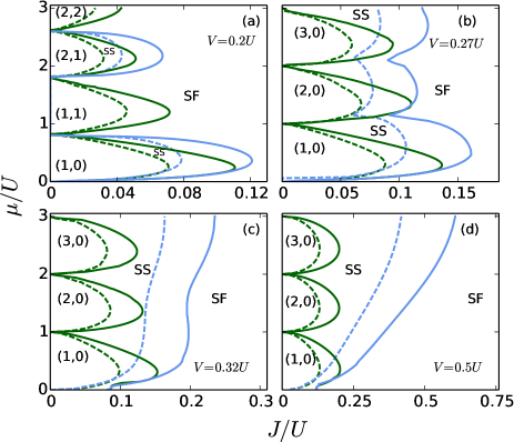
Figure 2: The phase diagrams of the eBHM obtained from the CGMF theory with $2\times 2$ clusters for uniform hopping amplitude ($J_{x}=J_{y}=J$) at $V/U=0.2,0.27,0.32$, and $0.5$ (a-d). The plots show the phase boundaries for two cases $\alpha=0$ and $\alpha=1/2$. The left dashed (solid) green line indicates the MI-SF, DW-SF and DW-SS phase boundaries for $\alpha=0$ ($\alpha=1/2$) case. The right dashed (solid) blue line represents the SS-SF phase boundary for $\alpha=0$ ($\alpha=1/2$) case. Here the DW and MI phases are indicated by their sublattice occupancies $(n_{A},n_{B})$.

The phase diagram of the eBHM obtained from the SGMF is as shown in Fig. 1 for different values of $V$. It is important to note that here $V$ is NN interaction which is $V_{1}$ of long-range interaction [Eq. (2)] and $V_{2}=0$. In the phase diagram, the incompressible DW and MI phases are identified by their sublattice occupancies $(n_{A},n_{B})$. We observed that for $zV<U$, where $z$ is the coordination number of the system, the ground state alternates between MI and DW phases, and regions of SS phase occur as envelopes around the DW phase lobes. On increasing $V$, at a critical value $zV_{c}=U$ the MI lobes are transformed into DW phase. For $V\geqslant V_{c}$, the SS phase occupies a larger region in the phase diagram. As $V$ is increased, the other observable effect is the critical value of the hopping strength $J_{c}/U$ for the DW-SS transition also increases. At higher values, when $zV\gtrsim 1.5U$, the SS-SF phase boundary is like a linear function of the $J$, and this is discernible from Fig. 1(d). In particular, the phase boundary is linear when $zJ/U>1$. These findings are in good agreement with the previous work of Iskin Iskin (2011). The numerical results of the phase boundaries are in good agreement with the analytical predictions of mean-field decoupling theory  Iskin (2012). For example, the critical hopping $J_{c}/U$ for DW(1,0) to SS transition at $V/U=0.32$ is $0.0994$ and analytical theory predicts the same value for these set of parameters. Similarly, we find the MI-SF phase boundaries from our study are consistent with the mean-field decoupling theory Iskin (2012). To examine the importance of the inter-site correlation effects the phase diagram using $2\times 2$ CGMF method is as shown in Fig. 2. It is qualitatively similar to the one based on SGMF in Fig. 1. But, there are several quantitative differences. First, the MI phase lobe is enhanced whereas DW phase lobe is suppressed. As an example, for $V/U=0.2$ the tip of the DW$(1,0)$ lobe is at $J_{c}/U=0.0717$ using SGMF theory, but with CGMF theory it is decreased to $0.0709$. Although, the difference between the $J_{c}$ using both theories is very small but using higher clusters CGMF one can get significant difference of $J_{c}$’s. This is apparent from the cluster finite-size scaling of the cluster sizes discussed in the next subsection. Second, at higher values of $V$ and $\alpha=1/2$, the SS-SF phase boundary commences at $J/U\approx 0$ and $\mu/U\approx 0$ with the SGMF theory. On the other hand, with the CGMF theory the SS-SF boundary starts at finite value of $J/U$ and $\mu/U=0$ [Fig. 2(c,d)]. Third, compared to the SGMF results, with the CGMF theory we obtain SS domains which are smaller in size. This is due to the better representation of fluctuations in the CGMF theory. Our results demonstrate the greater accuracy of the CGMF theory by correcting the overestimation of the SS domain obtained from the single-site mean-field theory. This observation is also consistent with similar comparison between results obtained from the single-site mean-field theory and quantum Monte Carlo (QMC) Ohgoe et al. (2012a); Flottat et al. (2017). And, finally, for higher values of $V/U$ the SS-SF boundary is linear at higher $\mu$ with SGMF theory. But, it is curved with the CGMF theory. Qualitatively, the value of $J_{c}$ obtained using SGMF and CGMF are close to the QMC results available in the literature. The value of $J_{c}/U$ of the DW(1,0) - SS quantum phase transition at $zV/U=1$ obtained using SGMF and CGMF methods are $0.0841$ and $0.0832$, respectively, and these values are close to QMC result of $0.0822$ Ohgoe et al. (2012a). Furthermore, we also carried out additional computations to compare the $J_{c}/U$ of DW-SF quantum phase transition at the half-filling with the QMC predictions Batrouni et al. (1995). For example, at $V/U\approx 0.35$, using SGMF we obtain $J_{c}/U=0.175$. Using CGMF theory this value is improved to $0.153$. And, this is in very good agreement with QMC result of $0.143$ reported in Ref. Batrouni et al. (1995). Further improvements in the values of the $J_{c}$ of various quantum phase transitions is possible when clusters of larger sizes are considered. This is also evident from the cluster finite-size scaling analysis discussed in next subsection.

As mentioned earlier, to study the effect of artificial gauge field, we choose $\alpha=1/2$. So, hereafter with artificial gauge field we mean $\alpha=1/2$. And, without artificial gauge field means $\alpha=0$. The artificial gauge field modifies the phase boundaries of MI, DW and SS phases, and the changes are discernible from the phase diagrams in Fig. 1. For example, for the $(1,0)$ DW lobe at $V/U=0.2$, the tip of the lobe is enhanced from $J_{c}/U\approx 0.0717$ by $40\%$ to $0.101$ with artificial gauge field. This enhancement in the insulating lobe and the phase boundaries of DW(MI) - SS(SF) transition with artificial gauge field are in agreement with the mean-field decoupling theory Iskin (2012). For example, the $J_{c}/U$ of DW(1,0)-SS quantum phase transition with $\alpha=1/2$ at $V/U=0.32$ is $0.1406$ which is same as the value obtained from the analytical theory Iskin (2012). The tip of the SS lobe is enhanced from $J_{c}/U\approx 0.084$ to $\approx 0.119$, and these changes together implies a larger domain of SS phase surrounding the DW(1,0) phase. These changes arise from the localizing effect of the Landau quantization, associated with the artificial gauge field, on the itinerant bosons. In addition, there are major differences between the SGMF and CGMF phase diagrams. For example, the tip of the $(1,0)$ DW lobe is increased from $J_{c}/U\approx 0.101$ in SGMF to $J_{c}/U=0.110$ in CGMF. This implies that the effect of correlation due to finite magnetic flux is better captured by the CGMF method. We perform the stability analysis of SS phase by computing the average occupancy $\langle n\rangle$ as a function of $\mu$  Sengupta et al. (2005); Flottat et al. (2017). The unstable phase is characterized by a discontinuity in $\langle n\rangle$ as $\mu$ is varied. In our study, we fix the $J/U$ and vary $\mu/U$ such that the SS phase is traversed, and then compute the average occupancy. As an example, at $J/U=0.12$ and $V/U=0.32$ for $\alpha=0$ case, we do not observe any discontinuity in $\langle n\rangle$ as a function of $\mu/U$. This confirms the stability of the SS phase of the soft-core bosons. We further include the NNN interaction term and find that the SS phase remains stable. The stability of soft-core SS phase is consistent with the QMC results of Ref. Sengupta et al. (2005); Ohgoe et al. (2012a). In addition, our analysis also demonstrates the stability of SS phase in the presence of the artificial gauge field.

To check the gauge-invariance of the phase boundaries, we also compute the phase boundaries for $\alpha\neq 0$ using SGMF and CGMF with the symmetric gauge. For the symmetric gauge, the vector potential $\mathbf{A(r)}=(1/2)(-By\hat{x}+Bx\hat{y})$. We observe that the phase boundaries obtained from the symmetric gauge are in good agreement with the results from Landau gauge. This can be seen from Fig.(1), where the filled black circles are the phase boundaries obtained using the symmetric gauge. For example, with the symmetric gauge, the tip of DW(1,0) lobe for $V/U=0.2$ is $J_{c}/U=0.101$ and which is identical with the Landau gauge result. Similarly, for the same value of $V/U$, the CGMF results with $2\times 2$ is $J_{c}/U=0.110$. And, this result is invariant under Landau and symmetric gauges. The SS-SF phase boundaries are also gauge-invariant as well. To illustrate, consider the SS-SF phase transition for $V/U=0.2$. With $\mu/U=0.44$, both the symmetric and Landau gauges give $J_{c}/U=0.119$. And, in the case of CGMF, the value $J_{c}/U=0.1207$ obtained with $2\times 2$ clusters is gauge invariant. Thus, the SGMF and CGMF methods give gauge-invariant phase boundaries for incompressible to compressible and SS-SF quantum phase transitions. This is consistent with the general principle that the observable quantities are gauge invariant Boada et al. (2010); Möller and Cooper (2010). And, it shows that the numerical methods we have used are robust as the results are gauge invariant.

Figure 3: The relative average occupancy of two consecutive sites are shown as a function of the chemical potential $\mu$ and hopping parameter $J$. The NN interaction is shown at the top of the figures.

The nature of the DW-SS transition is better represented by $\langle\Delta n\rangle$ and values for $V=0.22U$ and $0.32U$ corresponding to $V<V_{c}$ and $V>V_{c}$ are shown in Fig. 3. In the figure, the dark regions correspond to MI and SF phases and the region in other colors correspond to DW and SS phases. For $V=0.22U$, the regions in yellow color are DW phases and regions in other shades correspond to SS. The gradient in the shades indicates that the transition from DW to SS in terms of $\langle\Delta n\rangle$ is smooth. For the case of $V=0.32U$, there are no dark regions in the neighbourhood of $J/U\approx 0$. This is due to the absence of MI lobes, and is consistent with the phase diagram shown in Fig. 1 as all the MI lobes are transformed to DW lobes. The nature of the DW phases are apparent and visible from color gradient in Fig. 3 as the colors indicate the difference in the occupancy of two neighbouring lattice sites. As in the case of $V=0.22U$, regions with a color gradient indicate the SS phase and overall the relative average occupancy is in agreement with the phase diagram in Fig. 1. However, the phase diagram in terms of $\langle\Delta n\rangle$ provides a richer descriptions of the two phases, DW and SS, unique to the eBHM vis-a-vis BHM. And, the appropriate order parameter to examine the regions of SS phase.

Figure 4: The cluster finite-size scaling of $J_{c}$ for (1,1) MI-SF (blue) and (1,0) DW-SS (green) transition for different cluster sizes. The circles (triangles) represent the critical values obtained using periodic boundary conditions along both (one) spatial dimension. The square symbols represent the exact values in the thermodynamic limit. The scaling is performed for $\alpha=0$ and $V=0.2U$.

III.2 Cluster finite-size scaling

The results obtained from the SGMF and CGMF do provide qualitatively correct phase diagrams. And, this can further be improved using cluster finite-size scaling analysis. Such an analysis provides the location of the phase boundary in the thermodynamic limit. As a case study, we examine the location of the DW and MI lobe tips $J_{c}$ for $\alpha=0$, and $V=0.2U$. To implement the finite scaling analysis, we use a series of square and rectangular clusters $N_{\rm C}=2\times 2$, $4\times 2$, $6\times 2$, and $4\times 4$. In addition, we also include the results of $4\times 2$ and $4\times 4$ clusters with exact hopping along one spatial direction. Here, we consider clusters with even number of sites along $x$ and $y$ directions, as only these clusters generate checkerboard order. To obtain the thermodynamic limit, we introduce the scaling parameter $\lambda=N_{\rm B}/(N_{\rm B}+N_{\rm{\delta B}})$ which varies from $0$ to $1$. Here, $N_{\rm B}$ is the number of bonds within the cluster and $N_{\rm{\delta B}}$ is the number of bonds at the boundary which couples the cluster to it’s neighbours through the mean-field term  Yamamoto et al. (2012b); Lühmann (2013). The parameter $\lambda$ is a measure of the atomic correlations taken into account by using clusters of various sizes. In the extreme limits, the SGMF $N_{\rm C}=1\times 1$ and exact $N_{\rm C}=\infty$ results correspond to $\lambda=0$ and $\lambda=1$, respectively. Thus, the value of $J_{c}$ improves as $\lambda$ of the cluster approaches to $1$.

The cluster finite-size scaling analysis for the (1,0) DW and (1,1) MI phases with $\alpha=0$, and $V=0.2U$ are shown in Fig. 4. As seen from the figure, the location of the MI lobe tip $J_{c}$, increases with the cluster size. The SGMF favours the SF phase leading to underestimation of the MI phase. And, CGMF with larger cluster sizes enhance the MI lobe. Based on the linear fit the thermodynamic limit of $J_{c}$ is $0.05428$. One key feature is that, the results from the periodic boundary condition with exact hopping in one direction lie closer to the fitted line. And, more importantly, these have higher $\lambda$ as these have less bonds coupled to the mean field. The scaling behaviour of $J_{c}$ is in good agreement with the scaling results of MI-SF in BHM McIntosh et al. (2012); Lühmann (2013).

For the case of (1,0) DW phase, $J_{c}$ decreases with increasing cluster size. In other words, the domain with DW order shrinks with larger clusters and implies that SGMF theory overestimates DW order. This is corrected with the fluctuations incorporated with larger clusters. The trend is opposite to the MI phase case. From the cluster finite-size scaling analysis, the linear fit gives the thermodynamic limit of $J_{c}$ as $0.06021$. This trend of $J_{c}$ is also reported in earlier studies of hard-core eBHM Yamamoto et al. (2012a, b). Furthermore, the scaled $J_{c}$ values of eBHM phase boundaries at $zV/U=1$ are in good agreement with the QMC results Ohgoe et al. (2012a). In the presence of artificial gauge field, the qualitative features of the scaling analysis will be modified, and, the predicted exact critical values of the transitions will differ from the $\alpha=0$ case.

III.3 Finite temperature effects

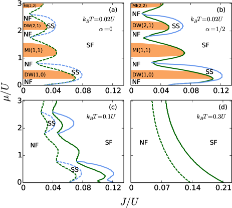
Figure 5: The finite temperature phase diagrams of eBHM obtained from CGMF theory with $2\times 2$ clusters. The orange striped region mark the DW and MI phases. (a) Phase diagram for $\alpha=0$ at $k_{B}T=0.02U$. The dashed green line marks MI-SF, NF-SF, DW-SS, and NF-SS phase boundaries. And, the dashed blue line marks the SS-SF phase boundary. (b) Phase diagram for $\alpha=1/2$ at $k_{B}T=0.02U$. The solid green line marks MI-SF, NF-SF, DW-SS, and NF-SS phase boundaries. And, the solid blue line marks the SS-SF phase boundary. Phase diagrams for $\alpha=0$ and $1/2$ at (c) $k_{B}T=0.1U$ and (d) $k_{B}T=0.3U$ with the combined color scheme of (a) and (b). Here, the NN interaction $V=0.2U$.

Thermal fluctuations associated with finite temperatures are an essential feature of experimental observations. Although the zero temperature phase diagrams do provide key insights and qualitative understanding, to relate with the experimental results it is essential to incorporate thermal fluctuations. We do this through the approach outlined in Section II.4. As mentioned earlier, the SS phase is yet to be observed in the eBHM and this could be due to the sensitivity of the phase to the thermal fluctuations. At zero temperature, SS phase appears in the system at a finite value of the NN interaction $V$. In Fig. 5, we show the finite temperature phase diagrams obtained using $2\times 2$ clusters in the CGMF method. As we have demonstrated and by others Buonsante et al. (2004); Yamamoto (2009); Pisarski et al. (2011); McIntosh et al. (2012); Lühmann (2013); Bai et al. (2018); Pal et al. (2019) that the results with CGMF are more reliable, hereafter we only consider the results from CGMF theory. From the plots in Fig. 5, a distinguishing feature of the thermal fluctuations is the emergence of the NF phase. The thermal fluctuation melts both the MI and DW phases and destroys the SF phase at the MI-DW or DW-DW boundaries.

To be more specific at $k_{B}T=0.02U$, as shown in Fig. 5(a-b), the orange stripes mark the DW and MI phases and the NF phase exist outside of these. The MI and NF both have zero $\phi$ and commensurate densities. The difference is that the MI has integer commensurate density, but NF has real commensurate density. The DW phase, on the other hand, has checkerboard density but with integer values. The NF region around the DW phase has incommensurate real density. By observing the local density variance or the compressibility, the incompressible DW and MI phases can be differentiated from NF phase as mentioned in Section II.5. On comparing the plots in Fig. 5(a) and Fig. 5(b), it is clear that the larger MI and DW lobes with finite $\alpha$ are retained at finite temperatures and hence the larger SS domain as well. At intermediate temperatures, both the MI and DW are entirely transformed into the NF phase but a portion of the SS lobes survives. This is visible in the phase diagram at $k_{B}T=0.1U$ shown in the Fig. 5(c). From the plots in the figure, the quantitative differences with and without the artificial gauge field is also visible. With artificial gauge field, the domain of the NF and SS phases are larger. For example, at $\mu=0$ the NF extends upto $J/U=0.064$ and $J/U=0.104$ for zero and finite $\alpha$, respectively. This trend of larger extent of NF phase with finite $\alpha$ extends to higher values of $\mu$. Upon further increase in temperature the crystalline order of the SS phase is destroyed and it vanishes from the phase diagram. At $k_{B}T\approx 0.3U$, as shown in Fig. 5(d), only the NF and SF phases are present in the system. At $\mu/U=0$ the NF-SF phase boundary is located at $J/U=0.136$ and $J/U=0.212$ for zero and finite $\alpha$, respectively. The separation between the location of the phase boundaries is reduced as $\mu/U$ increased. This is to be expected as the size of the DW lobes decrease with increasing $\mu/U$. As in the zero temperature case, the phase boundaries of the finite temperature phase diagrams are also gauge-invariant. We confirmed by analyzing the phase boundaries using symmetric gauge. As an illustration, consider the DW-SS transition at $\mu/U=0.4$ and $k_{B}T/U=0.02$ with $\alpha=1/2$, this point is chosen from the phase diagram in Fig. 5(b). We obtain $J_{c}/U=0.098$ using symmetric gauge and this value is in excellent agreement with the Landau gauge result. Similarly, for the same value of $\mu/U$ the SS-SF transition occurs at $J_{c}/U=0.122$ and this value is gauge-independent. At higher temperature, $k_{B}T/U=0.3$, the phase boundary of the NF-SF transition is also gauge-invariant. Hence, the comparison of $J_{c}/U$ for various quantum phase transitions using Landau and symmetric gauges demonstrate the gauge-invariance of the phase boundaries obtained with the numerical methods we have adopted in this work.

Figure 6: The zero temperature density distribution (upper panel) and SF order parameter (lower panel) of a $50\times 50$ square lattice for different values of dipolar interaction strengths $V/U$. The $V/U$ value is shown at the top of the figures. Here $x$ and $y$ are in units of the lattice spacing $a$.

III.4 Inhomogeneous case

The system considered so far is uniform and we emulate it with a $12\times 12$ lattice with periodic boundary conditions. However, in most of the quantum gas experiments the optical lattice has a confining envelope potential. Most often the external envelope potential is a harmonic oscillator. Hence, the inhomogeneity arising from this confining potential is another factor to be considered for comparison with the experimental observations. Therefore, we examine the ground-state of eBHM in a $50\times 50$ square lattice with SGMF theory. In which the external harmonic potential is incorporated in the chemical potential through the offset energy $\epsilon_{p,q}=\Omega(p^{2}+q^{2})$. Here $\Omega$ is the strength of the confining potential. The parameters of the system considered are $J/V=0.1$, $\mu/V=2.8$ and $\Omega/V=0.01$ Trefzger et al. (2008). The value of $\Omega$ is such that the atomic density outside the lattice potential is zero. The finite $\Omega$ modifies the local $\mu$ and therefore the ground state exhibits coexistence of various phases. Here $V$ is the strength of the dipolar interaction and the range of the potential is considered upto second nearest neighbours. Therefore, for the long-range interaction Eq. (2), $V_{1}=V$ and $V_{2}=V/2\sqrt{2}$.

To determine the changes in the competing phases we examine the ground state of the system at $V/U=0.05$, $0.5$, and $1.0$. These values cover the weak and strong limits of the dipolar interaction. In the experiments these regimes are reachable using Feshbach resonance in the dipolar atoms like Cr Werner et al. (2005), Er Frisch et al. (2014) and Dy Maier et al. (2015); Lucioni et al. (2018). As in the previous cases, to study the effects of the thermal fluctuations we consider three different values of $k_{B}T/V=0$, $0.2$, and $0.3$. At zero temperature, the profiles of $n_{p,q}$ and $\phi_{p,q}$ corresponding to $V/U=0.05$, $0.5$, and $1.0$ are shown in Fig. 6. For weak dipolar interaction $V/U=0.05$ the density is nearly uniform in the central region. The corresponding $\phi_{p,q}$ though nearly uniform shows a dip around the center. But, it is more uniform at the intermediate strength of the dipole interaction $0.5~{}U$. In both of these cases, $V/U=0.05$ and $0.5$, the central SF region is surrounded by the $(1,0)$ DW phase and this is evident from ring-shaped profile of the checkerboard density pattern in the figure. The other key feature is that the domain of the DW phase gets narrowed as $V/U$ is increased and above a critical value $V/U=0.8$ there is a quantum phase transition from DW phase to SS phase. This happens when both the interaction strengths, on-site and dipole interactions are comparable. As shown in Fig. 6, for $V/U=1$, there is a large region around the center where both the density and SF order parameter show checkerboard distributions. This is the signature of the SS phase.

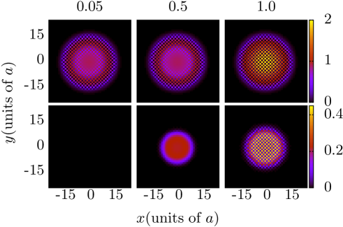
Figure 7: The density distribution (upper panel) and SF order parameter (lower panel) of a $50\times 50$ square lattice at $k_{B}T/V=0.2$ for different values of dipolar strengths $V/U$. The $V/U$ value is shown at the top of the figures. Here $x$ and $y$ are in units of the lattice spacing $a$.

Next, to relate to the experimental realizations we incorporate the finite temperature effects. For weak dipolar interaction the thermal fluctuations leads to the melting of the SF phase. This is evident from the density and SF order parameter corresponding to $V/U=0.05$ at $k_{B}T/V=0.2$ as shown in Fig. 7. A more detailed study, where $V/U$ is fixed and temperature is changed, shows that the SF phase at the central region does exist at lower temperatures. But, it melts to NF phase at the critical temperature of $k_{B}T/V=0.16$. At the higher value of $V/U=0.5$ the central SF region re-emerges and so does the SS phase at still higher value of $V/U=1$. In short, with thermal fluctuations it is essential to have stronger dipolar interactions to observe SS phase. Considering the parameters of the experimental realization of dipolar condensates of ¹⁶⁸Er in optical lattices Baier et al. (2016), the corresponding temperature of $k_{B}T/V=0.2$ is $\approx 40$ nK. This is within the experimental realm and hence, the combined effect of dipolar interaction and artificial gauge field can lead to the emergence of SS phase within experimentally achievable parameter domain.

At higher temperatures, $k_{B}T/V\approx 0.3$, the central region is in NF phase for weaker dipole interactions $V/U\leqslant 0.5$. Then, on increasing $V/U$ further the density assumes checkerboard pattern, but the SF order parameter is zero. That is the central region of the system is in the DW phase. This is to be compared and contrasted with the earlier result at $k_{B}T/V\approx 0.2$, where as shown in Fig. 7 the SS phase exists for $V/U=1$. Thus, focusing on the strong interaction domain $V/U=1$, our results show the existence of a SS-DW transition at $z~{}k_{B}T=V$. In short, the SS phase exists in the system at lower temperatures, but the SS order melts into DW phase when $z~{}k_{B}T\geqslant V$. On increasing the temperature further, the crystalline structure or diagonal long-range order of the DW phase starts to melt and at $z~{}k_{B}T\approx 3~{}V$ system is fully in the NF phase. So, the melting of the SS phase occurs in two steps. First, the off-diagonal long-range SF order is destroyed. This transforms the SS phase into DW phase. And, second, the DW phase melts into NF phase.

Figure 8: The density distribution (upper panel) and SF order parameter (lower panel) of a $50\times 50$ square lattice in the presence of artificial gauge field $\alpha=1/2$ at $k_{B}T/V=0.2$. The $V/U$ value is shown at the top of the figures. Here $x$ and $y$ are in units of the lattice spacing $a$.

In the presence of artificial gauge field the ground state and the corresponding SF order parameter at $k_{B}T/V=0.2$ are shown in Fig. 8. As in the case of uniform system, there are no qualitative changes in the results with the introduction of artificial gauge field, although the atoms have velocity current. For the parameters considered, at $\mu/V=2.8$ and $k_{B}T/V=0.2$, the SS phase appears in the range $\Delta J=0.04$, whereas in the presence of gauge field this range is enhanced to $\Delta J=0.07$. As discussed in the homogeneous case, for a given $\mu$ the range of $J$ for SS phase to occur is larger than without gauge field. This would enhance the possibility of observing the SS phase of eBHM in experimental realizations.

IV Conclusions

We have examined the zero and finite temperature phase diagrams of eBHM in 2D using SGMF and CGMF theory. In the presence of artificial gauge field the domain of SS phase is enhanced and $2\times 2$ CGMF theory provide better description of the system. The cluster finite-size scaling analysis demonstrates the key role of fluctuations in determining the quantum phases. For the DW-SS transition, the suppression of fluctuations favours the DW phase. But, in the MI-SF transition, suppression of fluctuations favours the SF phase. This is indicated by the decrease and increase of $J_{c}$ in the DW-SS and MI-SF transitions, respectively. At higher temperatures, the thermal fluctuations destroy the SS phase and the phase diagram exhibits NF-SF transition. Furthermore, we have studied the system of ultracold bosons with long range interactions in the presence of a harmonic confinement to relate with quantum gas experiments. Our results show that beyond a critical threshold of temperature $z~{}k_{B}T\geqslant V$, the SS phase vanishes and the system is occupied by the DW phase. These suggest that the prospect of observing the SS phase is higher when the temperature $z~{}k_{B}T<V$, this range of temperature is possible in the experiments of dipolar Bose gases loaded into optical lattices. This offers an opportunity to observe SS phase of eBHM in quantum dipolar gas experiments.