Context-Aware Zero-Shot Learning for Object Recognition

Abstract

Zero-Shot Learning (ZSL) aims at classifying unlabeled objects by leveraging auxiliary knowledge, such as semantic representations. A limitation of previous approaches is that only intrinsic properties of objects, e.g. their visual appearance, are taken into account while their context, e.g. the surrounding objects in the image, is ignored. Following the intuitive principle that objects tend to be found in certain contexts but not others, we propose a new and challenging approach, context-aware ZSL, that leverages semantic representations in a new way to model the conditional likelihood of an object to appear in a given context. Finally, through extensive experiments conducted on Visual Genome, we show that contextual information can substantially improve the standard ZSL approach and is robust to unbalanced classes.

1 Introduction

Traditional Computer Vision models, such as Convolutional Neural Networks (CNNs) (Lecun et al., 1998), are designed to classify images into a set of predefined classes. Their performances have kept improving in the last decade, namely on object recognition benchmarks such as ImageNet (Deng et al., 2009a), where state-of-the-art models (Zoph et al., 2017; Real et al., 2018) have outmatched humans. However, training such models requires hundreds of manually-labeled instances for each class, which is a tedious and costly acquisition process. Moreover, these models cannot replicate humans’ capacity to generalize and to recognize objects they have never seen before. As a response to these limitations, Zero-Shot Learning (ZSL) has emerged as an important research field in the last decade (Farhadi et al., 2009a; Mensink et al., 2012; Fu et al., 2015a; Kodirov et al., 2017). In the object recognition field, ZSL aims at labeling an instance of a class for which no supervised data is available, by using knowledge acquired from another disjoint set of classes, for which corresponding visual instances are provided. In the literature, these sets of classes are respectively called target and source domains — terms borrowed from the transfer learning community. Generalization from the source to the target domain is achieved using auxiliary knowledge that semantically relates classes of both domains, e.g. attributes or textual representations of the class labels.

Previous ZSL approaches only focus on intrinsic properties of objects, e.g. their visual appearance, by the means of handcrafted features — e.g. shape, texture, or color — (Lampert et al., 2014) or distributed representations learned from text corpora (Akata et al., 2016; Long et al., 2017). The underlying hypothesis is that the identification of entities of the target domain is made possible thanks to the implicit principle of compositionality (a.k.a. Frege’s principle (Pelletier, 2001)) — an object is formed by the composition of its attributes and characteristics — and the fact that other entities of the source domain share the same attributes. For example, if textual resources state that an apple is round and that it can be red or green, this knowledge can be used to identify apples in images because these characteristics (‘round‘, ‘red‘) could be shared by classes of the source domain (e.g, ‘round‘ like a ball, ‘red‘ like a strawberry…).

We believe that visual context, i.e. the other entities surrounding an object, also explains human’s ability to recognize an object that has never been seen before. This assumption relies on the fact that scenes are compositional in the sense that they are formed by the composition of objects they contain. Some works in Computer Vision have exploited visual context to refine the predictions of classification (Mensink et al., 2014) or detection (Bell et al., 2016) models. To the best of our knowledge, context has not been exploited in ZSL because, for obvious reasons, it is impossible to directly estimate the likelihood of a context for objects from the target domain — from visual data only. However, textual resources can be used to provide insights on the possible visual context in which an object is expected to appear. To illustrate this, knowing from language that an apple is likely to be found hanging on a tree or in the hand of someone eating it, can be very helpful to identify apples in images. In this paper, our goal is to leverage visual context as an additional source of knowledge for ZSL, by exploiting the distributed word representations (Mikolov et al., 2013) of the object class labels. More precisely, we adopt a probabilistic framework in which the probability to recognize a given object is split into three components: (1) a visual component based on its visual appearance (which can be derived from any traditional ZSL approach), (2) a contextual component exploiting its visual context, and (3) a prior component, which estimates the frequency of objects in the dataset. As a complementary contribution, we show that separating prior information in a dedicated component, along with simple yet effective sampling strategies, leads to a more interpretable model, able to deal with imbalanced datasets. Finally, as traditional ZSL datasets lack contextual information, we design a new dedicated setup based on the richly annotated Visual Genome dataset (Krishna et al., 2017). We conduct extensive experiments to thoroughly study the impact of contextual information.

2 Related work

Zero-shot learning

While state-of-the-art image classification models (Zoph et al., 2017; Real et al., 2018) restrict their predictions to a finite set of predefined classes, ZSL bypasses this important limitation by transferring knowledge acquired from seen classes (source domain) to unseen classes (target domain). Generalization is made possible through the medium of a common semantic space where all classes from both source and target domains are represented by vectors called semantic representations.

Historically, the first semantic representations that were used were handcrafted attributes (Farhadi et al., 2009a; Parikh & Grauman, 2011; Mensink et al., 2012; Lampert et al., 2014). In these works, the attributes of a given image are determined and the class with the most similar attributes is predicted. Most methods represent class labels with binary vectors of visual features (e.g, ’IsBlack’,’HasClaws’) (Lampert et al., 2009; Liu et al., 2011; Fu et al., 2014; Lampert et al., 2014). However, attribute-based methods do not scale efficiently since the attribute ontology is often domain-specific and has to be built manually. To cope with this limitation, more recent ZSL works rely on distributed semantic representations learned from textual datasets such as Wikipedia, using Distributional Semantic Models (Mikolov et al., 2013; Pennington et al., 2014; Peters et al., 2018). These models are based on the distributional hypothesis (Harris, 1954), which states that textual items with similar contexts in text corpora tend to have similar meanings. This is of particular interest in ZSL: all object classes (from both source and target domains) are embedded into the same continuous vector space based on their textual context, which is a rich source of semantic information. Some models directly aggregate textual representations of class labels and the predictions of a CNN (Norouzi et al., 2013), whereas others learn a cross-modal mapping between image representations (given by a CNN) and pre-learned semantic embeddings (Akata et al., 2015; Bucher et al., 2016). At inference, the predicted class of a given image is the nearest neighbor in the semantic embedding space. The cross-modal mapping is linear in most of ZSL works (Palatucci et al., 2009; Romera-Paredes & Torr, 2015; Akata et al., 2016; Qiao et al., 2016); this is the case in the present paper. Among these works, the DeViSE model (Frome et al., 2013) uses a max-margin ranking objective to learn a cross-modal projection and fine-tune the lower layers of the CNN. Several models have built upon DeViSE with approaches that learn non-linear mappings between the visual and textual modalities (Ba et al., 2015; Xian et al., 2016), or by using a common multimodal space to embed both images and object classes (Fu et al., 2015b; Long et al., 2017). In this paper, we extend DeViSE in two directions: by additionally leveraging visual context, and by reformulating it as a probabilistic model that allows coping with an imbalanced class distribution.

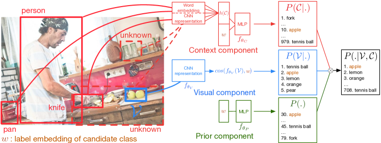
Figure 1: The goal is to find the class (in the target domain) of the object contained within the blue image region $\mathcal{V}$. Its context is formed of labeled objects from the source domain (red plain boxes) and of unlabeled object from the target domain (red dashed boxes).

Visual context

The intuitive principle that some objects tend to be found in some contexts but not others, is at the core of many works. In NLP, visual context of objects can be used to build efficient word representations (Zablocki et al., 2018). In Computer Vision, it can be used to refine detection (Chen et al., 2015; Chu & Cai, 2018) or segmentation (Zhang et al., 2018) tasks.

Visual context can either be low-level (i.e. raw image pixels) or high-level (i.e. labeled objects). When visual context is exploited in the form of low-level information (Torralba, 2003; Wolf & Bileschi, 2006; Torralba et al., 2010), it often consists of global image features. For instance, in (He et al., 2004), a Conditional Random Field is trained at combining low-level image features to assign to each pixel a class. In high-level approaches, the referential meaning of the context objects (i.e. class labels) is used. For example, Rabinovich et al. (2007) show that high-level context can be used at the post-processing level to reduce the ambiguities of a pre-learned object classification model, by leveraging co-occurrence patterns between objects that are computed from the training set. Moreover, Yu et al. (2016) study the role of context to classify objects: they investigate the importance of contextual indicators, such as object co-occurrence, relative scale and spatial relationships, and find that contextual information can sometimes be more informative than direct visual cues from objects. Spatial relations between objects can also be used in addition to co-occurrences, as in (Galleguillos et al., 2008; Chen et al., 2018). In (Bengio et al., 2013), co-occurrences are computed using external information collected from web documents. The model classifies all objects jointly; it gives an inference method enabling a balance between an image coherence term (given by an image classifier) and a semantic term (given by a co-occurrence matrix). However, the approach is fully supervised, and this setting cannot be applied to ZSL. The context-aware zero-shot learning task is related to the graph generation tasks (Zellers et al., 2018; Yang et al., 2018) and visual relationship detection (Lu et al., 2016).

In conclusion, while many works in NLP and Computer Vision show the importance of visual context, its use in ZSL remains a challenge, that we propose to tackle in this paper.

3 Context-aware Zero-Shot Learning

Let $\mathcal{O}$ be the set of all object classes, divided in classes from the source domain $\mathcal{S}$ and classes from the target domain $\mathcal{T}$. The goal of our approach — context-aware ZSL — is to determine the class $i\in\mathcal{T}$ of an object contained in an image $I$, given its visual appearance $\mathcal{V}$ and its visual context $\mathcal{C}$. The image $I$ is annotated with bounding boxes, each containing an object. Given the zone $\mathcal{V}$, the context $\mathcal{C}$ consists of the surrounding objects in the image. Their classes can either belong to the source domain ($\mathcal{C}\cap\mathcal{S}$) or to the target domain ($\mathcal{C}\cap\mathcal{T}$). Note that the class of an object of $\mathcal{C}\cap\mathcal{T}$ is not accessible in ZSL, only its visual appearance is.

3.1 Model overview

We tackle this task by modeling the conditional probability $P(i|\mathcal{V},\mathcal{C})$ of a class $i$ given both the visual appearance $\mathcal{V}$ and the visual context $\mathcal{C}$ of the object of interest. Given the absence of data in the target domain, we need to limit the complexity of the model, for generalizability’s purpose. Accordingly, we suppose that $\mathcal{V}$ and $\mathcal{C}$ are conditionally independent given the class $i$ — we show in the experiments (section 5) that this hypothesis is acceptable. This hypothesis leads to the following expression:

$$P(i|\mathcal{V},\mathcal{C})\propto P(\mathcal{V}|i)P(\mathcal{C}|i)P(i)$$ (1)

where each conditional probability expresses the probability of either the visual appearance $\mathcal{V}$ or the context $\mathcal{C}$ given class $i$, and $P(i)$ denotes the prior distribution of the dataset. Each term of this equation is modeled separately.

The intuition behind our approach is illustrated in Figure 1, where the blue box contains the object of interest. Here, the class is apple, which belongs to the target domain $\mathcal{T}$. The visual component, which focuses on the zone $\mathcal{V}$, recognizes a tennis ball due to its yellow and round appearance; apple is ranked second. The prior component indicates that apple is slightly more frequent than tennis ball, but the frequency discrepancy may not be high enough to change the prediction of the visual component. In that case, the context component is discriminant: it ranks objects that are likely to be found in a kitchen, and reveals that an apple is far more likely to be found than a tennis ball in this context.

Precisely modeling $P(\mathcal{C}|.)$, $P(\mathcal{V}|.)$ and $P(.)$ is challenging due to the ZSL setting. Indeed, these distributions cannot be computed for classes of the target domain because of the absence of corresponding training data. Thus, to transfer the knowledge acquired from the source domain to the target domain, we use a common semantic space, namely Word2Vec (Mikolov et al., 2013), where source and target class labels are embedded as vectors of $\mathbb{R}^{d}$, with $d$ the dimension of the space. It is worth noting that we propose to separately learn the prior class distribution $P(.)$ with a ranking loss (in section 3.3). This allows dealing with imbalanced datasets, in contrast to ZSL models like DeViSE (Frome et al., 2013). This intuition is experimentally validated in section 5.2.

3.2 Description of the model’s components

Due to both the ZSL setting and the variety of possible context and/or visual appearance of objects, it is not possible to estimate directly the different probabilities of equation 1. Hence, in what follows, we estimate quantities related to $P(\mathcal{C}|.)$, $P(\mathcal{V}|.)$ and $P(.)$ using parametric energy functions (LeCun et al., 2006). These quantities are learned separately, as described in section 3.3. Finally, we explain how we combine them to produce the global probability $P(.|\mathcal{C},\mathcal{V})$ in section 3.4.

Visual component

The visual component models $P(\mathcal{V}|i)$ by computing the compatibility between the visual appearance $\mathcal{V}$ of the object of interest, and the semantic representation $w_{i}$ of the class $i$.

Following previous ZSL works based on cross-modal projections (Frome et al., 2013; Bansal et al., 2018), we introduce $f_{\theta_{V}}$, a parametric function mapping an image to the semantic space: $f_{\theta_{V}}(\mathcal{V})=W_{V}.\texttt{CNN}(\mathcal{V})+b_{V}\in\mathbb{R}^{d}$ where $\texttt{CNN}(\mathcal{V})$ is a vector in $\mathbb{R}^{d_{\text{visual}}}$, output by a pretrained CNN truncated at the penultimate layer, $W_{V}$ is a projection matrix ($\in\mathbb{R}^{d\times d_{\text{visual}}}$) and $b_{V}$ a bias vector — in our experiments, $d_{\text{visual}}={2048}$. The probability that the image region $\mathcal{V}$ corresponds to the class $i$ is set to be proportional to the cosine similarity between the projection $f_{\theta_{V}}(\mathcal{V})$ of $\mathcal{V}$ and the semantic representation $w_{i}$ of $i$:

$$\log P(\mathcal{V}|i;\theta_{V})\propto\cos(f_{\theta_{V}}(\mathcal{V}),w_{i}):=\log\widetilde{P}_{\textit{visual}}$$ (2)

Context component

The context component models $P(\mathcal{C}|i)$ by computing a compatibility score between the visual context $\mathcal{C}$, and the semantic representation $w_{i}$ of class $i$. More precisely, the conditional probability is written:

$$\log P(\mathcal{C}|i;\theta_{C})\propto f_{\theta_{C}}(\mathcal{C},w_{i}) =f_{\theta^{1}_{C}}\big{(}h_{\theta^{2}_{C}}(\mathcal{C})\oplus w_{i}\big{)}$$

$$:=\log\widetilde{P}_{\textit{context}}$$ (3)

where $h_{\theta^{2}_{C}}(\mathcal{C})\in\mathbb{R}^{d}$ is a vector representing the context, $\theta_{C}=\{\theta^{1}_{\mathcal{C}};\theta^{2}_{\mathcal{C}}\}$ are parameters to learn, and $\oplus$ is the concatenation operator. To take non-linear and high-order interactions between $h_{\theta^{2}_{C}}(\mathcal{C})$ and $w_{i}$ into account, $f_{\theta_{C}^{1}}$ is modeled by a 2-layer Perceptron. We found that concatenating $h_{\theta_{C}^{2}}(\mathcal{C})$ with $w_{i}$ leads to better results than a cosine similarity, as done in equation 2 for the visual component.

To specify the modeling of $h_{\theta^{2}_{C}}(\mathcal{C})$, we propose various context models depending on which context objects are considered and how they are represented. Specifically, a context model is characterized by (a) the domain of context objects that are considered (i.e. source $\mathcal{S}$ or target $\mathcal{T}$) and (b) the way these objects are represented, either by a textual representation of their class label or by a visual representation of their image regions. Accordingly, we distinguish:
$\bullet$ The low-level ($L$) approach that computes a representation from the image region $\mathcal{V}_{k}$ of a context object. This produces the following context models:

$$S_{L}=\{W_{C}\texttt{CNN}(\mathcal{V}_{k})+b_{C}|k\in\mathcal{C}\cap\mathcal{S}\}$$

$$T_{L}=\{W_{C}\texttt{CNN}(\mathcal{V}_{k})+b_{C}|k\in\mathcal{C}\cap\mathcal{T}\}$$

$\bullet$ The high-level ($H$) approach which considers semantic representations $w_{k}$ of the class labels $k$ of the context objects (only available for entities of the source domain). This produces context models:

$$S_{H}=\{w_{k}|k\in\mathcal{C}\cap\mathcal{S}\}\mbox{ and }T_{H}=\{w_{k}|k\in\mathcal{C}\cap\mathcal{T}\}$$

Note that $T_{H}$ is not defined in the zero-shot setting, since class labels of objects from the target domain are unknown; yet it is used to define Oracle models (section 4.3).

These four basic sets of vectors can further be combined in various ways to form new context models (for instance: $S_{L}\cup T_{L},S_{H}\cup S_{L},S_{H}\cup S_{L}\cup T_{L}$, etc.). At last, $h_{\theta_{C}^{2}}$ averages the representations of these vectors to build a global context representation. For example, $h_{\theta_{C}^{2}}(\mathcal{C}_{S_{H}\cup T_{L}})$ equals:

$$\frac{1}{|\mathcal{C}_{\mathcal{S}}|+|\mathcal{C}_{\mathcal{T}}|}\Big{[}\sum\limits_{(i,\mathcal{V}_{i})\in\mathcal{C}_{\mathcal{S}}}w_{i}+\sum\limits_{(j,\mathcal{V}_{j})\in\mathcal{C}_{\mathcal{T}}}\big{(}W_{C}.\texttt{CNN}(\mathcal{V}_{j})+b_{C}\big{)}\Big{]}$$

where $|\cdot|$ denotes the cardinality of a set of vectors.

Prior component

The goal of the prior component is to assess whether an entity is frequent or not in images. We estimate $P(i)$ from the semantic representation $w_{i}$ of class $i$:

$$\log P(i;\theta_{P})\propto f_{\theta_{P}}(w_{i}):=\log\widetilde{P}_{\textit{prior}}$$ (4)

where $f_{\theta_{P}}$ is a 2-layer Perceptron that outputs a scalar.

3.3 Learning

In this section, we explain how we learn the energy functions $f_{\theta_{C}}$, $f_{\theta_{V}}$ and $f_{\theta_{P}}$. Each component (resp. context, visual, prior) of our model is assigned a training objective (resp. $\mathcal{L}_{C}$, $\mathcal{L}_{V}$, $\mathcal{L}_{P}$). As the components are independent by design, they are learned separately. This allows for a better generalization in the target domain, as shown experimentally (section 5.2). Besides, ensuring that some configurations are more likely than others motivates us to model each objective by a max-margin ranking loss, in which a positive configuration is assigned a lower energy than a negative one, following the learning to rank paradigm (Weston et al., 2011). Unlike previous works (Frome et al., 2013), which are generally based on balanced datasets such as ImageNet and thus are not concerned with prior information, we want to avoid any bias coming from the imbalance of the dataset in $\mathcal{L}_{C}$ and $\mathcal{L}_{V}$, and learn the prior separately with $\mathcal{L}_{P}$. In other terms, the visual (resp. context) component should focus exclusively on the visual appearance (resp. visual context) of objects. This is done with a careful sampling strategy of the negative examples within the ranking objectives, that we detail in the following. To the best of our knowledge, such a discussion relative to prior modeling in learning objectives — which is, in our view, paramount in imbalanced datasets such as Visual Genome — has not been done in previous research.

Positive examples are sampled among entities of the source domain from the data distribution $P^{\star}$: they consist in a single object for $\mathcal{L}_{P}$, an object/box pair for $\mathcal{L}_{V}$, an object/context pair for $\mathcal{L}_{C}$. To sample negative examples $j$ from the source domain, we distinguish two ways:

(1) For the prior objective $\mathcal{L}_{P}$, negative object classes are sampled from the uniform distribution $U$:

$$\mathcal{L}_{P}=\mathop{\mathbb{E}}\limits_{i\sim P^{\star}}\mathop{\mathbb{E}}\limits_{j\sim U}\big{\lfloor}\gamma_{P}-f_{\theta_{P}}(w_{i})+f_{\theta_{P}}(w_{j})\big{\rfloor}_{+}$$ (5)

Noting $\Delta_{ji}:=f_{\theta_{P}}(w_{j})-f_{\theta_{P}}(w_{i})$, the contribution of two given objects $i$ and $j$ to this objective is:

$$P^{\star}(i)\big{\lfloor}\gamma_{P}+\Delta_{ji}\big{\rfloor}_{+}+P^{\star}(j)\big{\lfloor}\gamma_{P}-\Delta_{ji}\big{\rfloor}_{+}$$

If $P^{\star}(i)>P^{\star}(j)$, i.e. when object class $i$ is more frequent than object class $j$, this term is minimized when $\Delta_{ji}=-\gamma_{P}$, i.e. $f_{\theta_{P}}(w_{i})=f_{\theta_{P}}(w_{j})+\gamma_{P}>f_{\theta_{P}}(w_{j})$. Thus, $\widetilde{P}_{\textit{prior}}(.;\theta_{P})$ captures prior information, as it learns to rank objects based on their frequency.

(2) For the visual and context objectives, negative object classes are sampled from the prior distribution $P^{\star}(.)$:

$$\mathcal{L}_{V} =\mathop{\mathbb{E}}\limits_{i,\mathcal{V}\sim P^{\star}}\mathop{\mathbb{E}}\limits_{j\sim P^{\star}}\big{\lfloor}\gamma_{V}-f_{\theta_{V}}(\mathcal{V})^{\top}w_{i}+f_{\theta_{V}}(\mathcal{V})^{\top}w_{j}\big{\rfloor}_{+}$$ (6)

$$\mathcal{L}_{C} =\mathop{\mathbb{E}}\limits_{i,\mathcal{C}\sim P^{\star}}\mathop{\mathbb{E}}\limits_{j\sim P^{\star}}\big{\lfloor}\gamma_{C}-f_{\theta_{C}}\big{(}\mathcal{C},w_{i}\big{)}+f_{\theta_{C}}\big{(}\mathcal{C},w_{j}\big{)}\big{\rfloor}_{+}$$ (7)

Similarly, the contribution of two given objects $i$, $j$ and a context $\mathcal{C}$ to the objective $\mathcal{L}_{C}$ is:

$$P^{\star}(i)P^{\star}(j)\Big{[}P^{\star}(\mathcal{C}|i)\big{\lfloor}\gamma_{V}+f_{\theta_{C}}(\mathcal{C},w_{j})-f_{\theta_{C}}(\mathcal{C},w_{i})\big{\rfloor}_{+}$$

$$+P^{\star}(\mathcal{C}|j)\big{\lfloor}\gamma_{V}+f_{\theta_{C}}(\mathcal{C},w_{i})-f_{\theta_{C}}(\mathcal{C},w_{j})\big{\rfloor}_{+}\Big{]}$$

Minimizing this term does not depend on the relative order between $P^{\star}(i)$ and $P^{\star}(j)$; thus, $\widetilde{P}_{\textit{context}}(\mathcal{C}|.;\theta_{C})$ does not take prior information into account. Moreover, ${P^{\star}(\mathcal{C}|i)>P^{\star}(\mathcal{C}|j)}$ implies that $f_{\theta_{C}}(\mathcal{C},w_{i})>f_{\theta_{C}}(\mathcal{C},w_{j})$.

The alternative, as done in DeViSE (Frome et al., 2013), is to sample negative classes uniformly in the source domain in the objective $\mathcal{L}_{V}$. Thus, if the prior is uniform, DeViSE directly models $P(.|\mathcal{V})$; otherwise, $\mathcal{L}_{V}$ cannot be analyzed straightforwardly. Besides, the contributions of visual and prior information are mixed. However, we show that learning the prior separately and imposing the context (resp. visual) component to exclusively focus on contextual (resp. visual) information is more efficient (section 5.2).

3.4 Inference

In this section, we detail the inference process. The goal is to combine the predictions of the individual components of the model to form the global probability distribution $P(.|\mathcal{V},\mathcal{C})$. In section 3.3, we detailed how to learn the functions $f_{\theta_{C}}$, $f_{\theta_{V}}$ and $f_{\theta_{P}}$, from which $\log\widetilde{P}_{\textit{context}}$, $\log\widetilde{P}_{\textit{visual}}$ and $\log\widetilde{P}_{\textit{prior}}$ are deduced respectively. However, the normalization constants in equations 2, 3 and 4, which depend on the object class $i$ in the general case, are unknown. As a simplifying hypothesis, we suppose that these normalization constants are scalars that we respectively note $\alpha_{C}$, $\alpha_{V}$ and $\alpha_{P}$. This leads to:

$$P(.|\mathcal{V},\mathcal{C})=\underbrace{(\widetilde{P}_{\textit{context}})^{\alpha_{C}}}_{\textstyle P(\mathcal{C}|.)}.\underbrace{(\widetilde{P}_{\textit{visual}})^{\alpha_{V}}}_{\textstyle P(\mathcal{V}|.)}.\underbrace{(\widetilde{P}_{\textit{prior}})^{\alpha_{P}}}_{\textstyle P(.)}$$ (8)

To see whether this hypothesis is reasonable, we did some post-hoc analysis of one of our model, and plotted in Figure 2 the values $\log\widetilde{P}_{\textit{visual}}$, $\log\widetilde{P}_{\textit{context}}$ and $\log\widetilde{P}_{\textit{prior}}$ for positive (red points) and negative (blue points) configurations $(i,\mathcal{V},\mathcal{C})$ of the test set of Visual Genome. We observe that positive and negative triplets are well separated, which empirically validates our initial hypothesis.

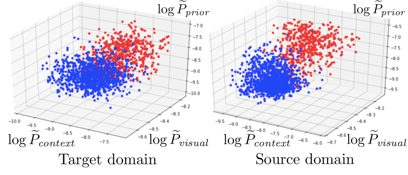
Figure 2: 3D visualization of the unnormalized log-probabilities of each component ($N=500$). Context model ${S_{L}\cup S_{H}\cup T_{L}}$.

Hyper-parameters $\alpha_{C},\alpha_{V}$ and $\alpha_{P}$ are selected on the validation set to compute $P(.|\mathcal{C},\mathcal{V})$. To build models that do not use a visual/contextual component, we simply select a subset of the probabilities and their respective hyperparameters. For example, $P(.|\mathcal{C})=(\widetilde{P}_{\textit{context}})^{\alpha_{C}}(\widetilde{P}_{\textit{prior}})^{\alpha_{P}}$.

4 Experimental protocol

4.1 Data

To measure the role of context in ZSL, a dataset that presents annotated objects within a rich visual context is required. However, traditional ZSL datasets, such as AwA (Farhadi et al., 2009b), CUB-200 (Wah et al., 2011) or LAD (Zhao et al., 2018), are made of images that contain a unique object each, with no or very little surrounding visual context. We rather use Visual Genome (Krishna et al., 2017), a large-scale image dataset (108K images) annotated at a fine-grained level (3.8M object instances), covering various concepts (105K unique object names). This dataset is of particular interest for our work, as objects have richly annotated contexts ($31$ object instances per image on average). In order to shape the data to our task, we randomly split the set of images of Visual Genome into train/validation/test sets (70%/10%/20% of the total size). To build the set $\mathcal{O}$ of all objects classes, we select classes which appear at least 10 times in Visual Genome and have an available Word2vec representation. $\mathcal{O}$ contains $4842$ object classes; it amounts to 3.4M object instances in the dataset. This dataset is highly imbalanced as 10% of most represented classes amount to 84% of object instances. We define the level of supervision $p_{\text{sup}}$ as the ratio of the size of the source domain over the total number of objects: $p_{\text{sup}}=|\mathcal{S}|/|\mathcal{O}|$. For a given $p_{\text{sup}}$ ratio, the source $\mathcal{S}$ and target $\mathcal{T}$ domains are built by randomly splitting $\mathcal{O}$ accordingly. Every object is annotated with a bounding box and we use this supervision in our model for entities of both source and target domains. To facilitate future work on context-aware ZSL, we publicly release data splits and annotations .

4.2 Evaluation methodology and metrics

We adopt the conventional setting for ZSL, which implies entities to be retrieved only among the target domain $\mathcal{T}$. Besides, we also evaluate the performance of the model to retrieve entities of the source domain $\mathcal{S}$ (with models tuned on the target domain).

The model’s prediction takes the form of a list of $n$ classes, sorted by probability; the rank of the correct class in that list is noted $r$. Depending on the setting, $n$ equals $|\mathcal{T}|$ or $|\mathcal{S}|$. We define the First Relevant (FR) metric with ${\text{FR}=\frac{2}{n-1}(r-1)}$. To further evaluate the performance over the whole test set, the Mean First Relevant (MFR) metric is used (Fuhr, 2017). It is computed by taking the mean value of FR scores obtained on each image of the test set. Note that the factor $\frac{2}{n-1}$ rescales the metric such that the MFR score of a random baseline is 100%, while the MFR of a perfect model would be 0%. The MFR metric has the advantage to be interval-scale-based, unlike more traditional Recall@$k$ metrics or Mean Reciprocal Ranks metrics (Ferrante et al., 2017), and thus can be averaged; this allows for meaningful comparison with a varying $p_{\text{sup}}$.

4.3 Scenarios and Baselines

Model scenarios

Model scenarios depend on the information that is used in the probabilistic setting: $\varnothing$, $\mathcal{C}$, $\mathcal{V}$ or both $\mathcal{C}$ and $\mathcal{V}$. When contextual information is involved, a context model $\star$ is specified to represent $\mathcal{C}$, which we note $\mathcal{C}_{\star}$. The different context models are $\star\in\{S_{H},S_{L},T_{L},S_{L}\cup T_{L},S_{H}\cup T_{L},S_{L}\cup S_{H}\cup T_{L}\}$. For clarity’s sake, we note our model M. For example, M$(\mathcal{C}_{S_{H}\cup T_{L}},\mathcal{V})$ models the probability $P(\mathcal{C}_{S_{H}\cup T_{L}}|.)P(\mathcal{V}|.)P(.)$ as explained in 3.4, M$(\mathcal{V})$ models $P(\mathcal{V}|.)P(.)$, and M$(\varnothing)$ models $P(.)$.

Oracles

To evaluate upper-limit performances for our models, we define Oracle baselines where classes of target objects are used, which is not allowed in the zero-shot setting. Note that every Oracle leverages visual information.
$\bullet$ True Prior: This Oracle uses, for its prior component, the true prior distribution $P^{\star}(i)=\frac{\#i}{M}$ computed for all objects of both source and target domains on the full dataset, where $\#i$ is the number of instances of the $i$-th class in images and $M$ is the total number of images.
$\bullet$ Visual Bayes: This Oracle uses $P^{\star}(.)$ for its prior component as well. Its context component uses co-occurrence statistics between objects computed on the full dataset: $P^{\text{im}}(\mathcal{C}|i)=\prod_{c\in\mathcal{C}}P_{\text{co-oc}}(c|i)$ where $P_{\text{co-oc}}(c|i)=\frac{\#(c,i)M}{\#c\#i}$ is the probability that objects $c$ and $i$ co-occur in images, with $\#(c,i)$ the number of co-occurrences of $c$ and $i$.
$\bullet$ Textual Bayes: Inspired by (Bengio et al., 2013), this Oracle is similar to Visual Bayes, except that its prior $P^{\text{text}}(.)$ and context component $P^{\text{text}}(.|\mathcal{C})$ are based on textual co-occurrences instead of image co-occurrences: $P_{\text{co-oc}}(c|i)$ is computed by counting co-occurrences of words $c$ and $i$ in windows of size 8 in the Wikipedia dataset, and $P^{\text{text}}(i)$ is computed by summing the number of instances of the $i$-th class divided by the total size of Wikipedia.
$\bullet$ Semantic representations for all objects: M$(\mathcal{C}_{S_{H}\cup T_{H}},\mathcal{V})$ uses word embeddings of both source and target objects.

Baselines
$\bullet$ M$(\mathcal{C}\oplus\mathcal{V}$): To study the validity of the hypothesis about the conditional independence of $\mathcal{C}$ and $\mathcal{V}$, we introduce a baseline where we directly model $P(\mathcal{C},\mathcal{V}|.)P(.)$. To do so, we replace, in the expression of $\mathcal{L}_{V}$ (equation 6), $f_{\theta_{V}}(\mathcal{V})$ by the concatenation of $h(\mathcal{C})$ and $f_{\theta_{V}}(\mathcal{V})$ projected in $\mathbb{R}^{d}$ with a 2-layer Perceptron.
$\bullet$ DeViSE$(\mathcal{V})$: To evaluate the impact of our Bayesian model (equation 1) and our sampling strategy (section 3.3), we compare against DeViSE (Frome et al., 2013). DeViSE$(\mathcal{V})$ is different from M$(\mathcal{V})$ because negative examples in $\mathcal{L}_{V}$ are uniformly sampled, and the prior $P(.)$ is not learned.
$\bullet$ DeViSE$(\mathcal{C}\oplus\mathcal{V})$: similarly to M$(\mathcal{C}\oplus\mathcal{V})$, we define a baseline that does not rely on the conditional independence of $\mathcal{C}$ and $\mathcal{V}$, using the same sampling strategy as DeViSE.
$\bullet$ M$(\mathcal{C}_{I},\mathcal{V})$: To understand the importance of context supervision, i.e. annotations of context objects (boxes and classes), we design a baseline where no context annotations are used. The context is the whole image without the zone $\mathcal{V}$ of the object, which is masked out. The associated context model is $\star=I$ with $h(\mathcal{C_{I}})=g_{\theta_{I}}(I\setminus\mathcal{V})$ ; $g_{\theta_{I}}$ is a parametric function to be learned. This baseline is inspired from (Torralba et al., 2010), where global image features are used to refine the prediction of an image model.

4.4 Implementation details

For each objective $\mathcal{L}_{C},\mathcal{L}_{V}$ and $\mathcal{L}_{P}$, at each iteration of the learning algorithm, 5 negative entities are sampled per positive example. Word representations are vectors of $\mathbb{R}^{300}$, learned with the Skip-Gram algorithm (Mikolov et al., 2013) on Wikipedia. Image regions are cropped, rescaled to (299$\times$299), and fed to CNN, an Inception-v3 CNN (Szegedy et al., 2016), whose weights are kept fixed during training. This model is pretrained on ImageNet (Deng et al., 2009b). As a result, every ImageNet class that belongs to the total set of objects $\mathcal{O}$ was included in the source domain $\mathcal{S}$. Models are trained with Adam (Kingma & Ba, 2014) and regularized with a L2-penalty; the weight of this penalty decreases when the level of supervision increases, as the model is less prone to overfitting. All hyper-parameters are cross-validated on classes of the target domain, on the validation set.

5 Results

Table 1: Evaluation of various information sources, with varying levels of supervision. MFR scores in $\%$. $\delta_{C}$ is the relative improvement (in $\%$) of M$(\mathcal{C}_{S_{H}},\mathcal{V})$ over M$(\mathcal{V})$.

		Target domain $\mathcal{T}$			Source domain $\mathcal{S}$
	$p_{\text{sup}}$	10%	50%	90%	10%	50%	90%
	Domain size	4358	2421	484	484	2421	4358
Models	Random	100	100	100	100	100	100
	M$(\varnothing)$	38.6	23.7	13.8	12.0	10.6	11.2
	M$(\mathcal{V})$	20.5	10.7	6.0	1.5	2.6	3.6
	M$(\mathcal{C}_{S_{H}})$	28.7	14.4	9.1	4.2	4.3	4.4
	M$(\mathcal{C}_{S_{H}},\mathcal{V})$	18.1	9.0	5.2	1.1	1.9	2.4
	$\delta_{\mathcal{C}}$ (%)	11.6	16.4	12.1	23.7	27.3	31.5

5.1 The importance of context

In this section, we evaluate the contribution of contextual information, with varying levels of supervision $p_{\text{sup}}$. We fix a simple context model ($\star=S_{H}$) and report MFR results with $p_{\text{sup}}=10,50,90\%$ in Table 1 for every combination of information sources: $\varnothing$, $\mathcal{V}$, $\mathcal{C}$ and $(\mathcal{C},\mathcal{V})$ — we observe similar trends for the other context models. Results highlight that contextual knowledge acquired from the source domain can be transferred to the target domain, as M$(\mathcal{C}_{S_{H}})$ significantly outperforms the Random baseline. As expected, it is not as useful as visual information: M$(\mathcal{V})\stackrel{{\scriptstyle\text{MFR}}}{{\smash{{\scalebox{0.8}{\textless}}}}}$ M$(\mathcal{C}_{S_{H}})$, where $\stackrel{{\scriptstyle\text{MFR}}}{{\smash{{\scalebox{0.8}{\textless}}}}}$ means lower MFR scores, i.e. better performances. However, Table 1 demonstrates that contextual and visual information are complementary: using M$(\mathcal{C}_{S_{H}},\mathcal{V})$ outperforms both M$(\mathcal{C}_{S_{H}})$ and M$(\mathcal{V})$. Interestingly, as the learned prior model M$(\varnothing)$ is also able to generalize, we show that visual frequency can somehow be learned from textual semantics, which extends previous work where word embeddings were shown to be a good predictor of textual frequency (Schakel & Wilson, 2015).

When $p_{\text{sup}}$ increases, we observe that all models are better at retrieving objects of the target domain (i.e. MFR decreases), which is intuitive because models are trained on more data and thus generalize better to recognize entities from the target domain. Besides, when $p_{\text{sup}}$ increases, the context is also more abundant. This explains: (1) the decreasing MFR values for model M$(\mathcal{C}_{S_{H}})$ on $\mathcal{T}$, (2) the increasing relative improvement $\delta_{C}$ of M$(\mathcal{C}_{S_{H}},\mathcal{V})$ over M$(\mathcal{V})$ on $\mathcal{S}$. However, on the target domain, we note that $\delta_{C}$ does not monotonously increase with $p_{\text{sup}}$. A possible explanation is that the visual component improves faster than the context component, so the relative contribution brought by context to the final model M$(\mathcal{C}_{S_{H}},\mathcal{V})$ decreases after $p_{\text{sup}}=50\%$. Since the highest relative improvement $\delta_{C}$ (in $\mathcal{T}$) is attained with $p_{\text{sup}}=50\%$, we fix the standard level of supervision $p_{\text{sup}}=50\%$ in the rest of the experiments; this amounts to 2421 classes in both source and target domains.

5.2 Modeling contextual information

Table 2: MFR performances (given in $\%$) for all baselines and scenarios. $p_{\text{sup}}=50\%$. Oracle results, written in italics, are not taken into account to determine the best scores, written in bold.

	Model	Probability	$\mathcal{T}$	$\mathcal{S}$
Oracles	Textual Bayes	$P^{\text{text}}(\mathcal{C}|.)P(\mathcal{V}|.)P^{\text{text}}(.)$	14.54	6.73
	M$(\mathcal{C}_{S_{H}\cup T_{H}},\mathcal{V})$	$P(\mathcal{C}_{S_{H}\cup T_{H}}|.)P(\mathcal{V}|.)P(.)$	7.57	2.53
	True Prior	$P(\mathcal{V}|.)P^{\star}(.)$	4.92	2.63
	Visual Bayes	$P^{\text{im}}(\mathcal{C}|.)P(\mathcal{V}|.)P^{\star}(.)$	3.40	2.11
Baselines	DeViSE$(\mathcal{V})$	$P(.|\mathcal{V})$	10.73	3.62
	DeViSE$(\mathcal{C}_{S_{H}}\oplus\mathcal{V})$	$P(.|\mathcal{C}_{S_{H}},\mathcal{V})$	10.11	3.11
	M$(\mathcal{C}_{S_{H}}\oplus\mathcal{V})$	$P(\mathcal{C}_{S_{H}},\mathcal{V}|.)P(.)$	10.07	1.85
	M$(\mathcal{C}_{I},\mathcal{V})$	$P(\mathcal{C}_{I}|.)P(\mathcal{V}|.)P(.)$	9.19	2.13
Our models	M$(\mathcal{V})$	$P(\mathcal{V}|.)P(.)$	10.72	2.64
	M$(\mathcal{C}_{S_{L}},\mathcal{V})$	$P(\mathcal{C}_{S_{L}}|.)P(\mathcal{V}|.)P(.)$	9.01	2.05
	M$(\mathcal{C}_{T_{L}},\mathcal{V})$	$P(\mathcal{C}_{T_{L}}|.)P(\mathcal{V}|.)P(.)$	9.00	2.13
	M$(\mathcal{C}_{S_{H}},\mathcal{V})$	$P(\mathcal{C}_{S_{H}}|.)P(\mathcal{V}|.)P(.)$	8.96	1.92
	M$(\mathcal{C}_{S_{H}\cup S_{L}},\mathcal{V})$	$P(\mathcal{C}_{S_{H}\cup S_{L}}|.)P(\mathcal{V}|.)P(.)$	8.71	1.88
	M$(\mathcal{C}_{S_{L}\cup T_{L}},\mathcal{V})$	$P(\mathcal{C}_{S_{L}\cup T_{L}}|.)P(\mathcal{V}|.)P(.)$	8.60	1.93
	M$(\mathcal{C}_{S_{H}\cup T_{L}},\mathcal{V})$	$P(\mathcal{C}_{S_{H}\cup T_{L}}|.)P(\mathcal{V}|.)P(.)$	8.52	1.86
	M$(\mathcal{C}_{S_{H}\cup S_{L}\cup T_{L}},\mathcal{V})$	$P(\mathcal{C}_{S_{H}\cup S_{L}\cup T_{L}}|.)P(\mathcal{V}|.)P(.)$	8.31	1.79

In this section, we compare the different context models; results are reported in Table 2. First, underlying hypotheses of our model are experimentally tested. (1) Modeling context and prior information with semantic representations (models M$(\mathcal{C}_{\star},\mathcal{V}))$ is far more efficient than using direct textual co-occurrences, as shown by the Textual Bayes baseline, which is the weaker model despite being an Oracle. (2) Moreover, we show that the hypothesis on the conditional independence of $\mathcal{C}$ and $\mathcal{V}$ is acceptable, as separately modeling $\mathcal{C}$ and $\mathcal{V}$ gives better results than jointly modeling them (i.e. M$(\mathcal{C}_{S_{H}},\mathcal{V})$ $\stackrel{{\scriptstyle\text{MFR}}}{{\smash{{\scalebox{0.8}{\textless}}}}}$ M$(\mathcal{C}_{S_{H}}\oplus\mathcal{V})$). (3) Furthermore, we observe that our approach M$(\mathcal{V}$) is more efficient to capture the imbalanced class distribution of the source domain, compared to DeViSE$(\mathcal{V})$; indeed, True Prior $\approx$ M$(\mathcal{V})$ , whereas True Prior $\stackrel{{\scriptstyle\text{MFR}}}{{\smash{{\scalebox{0.8}{\textless}}}}}$ DeViSE$(\mathcal{V})$ on $\mathcal{S}$. Even if the improvement is only significant for the source domain $\mathcal{S}$, it indicates that separately using information sources is clearly a superior approach to further integrate contextual information.

Second, as observed in the case of the context model $S_{H}$ (section 5.1), using contextual information is always beneficial. Indeed, all models with context M$(\mathcal{C}_{\star},\mathcal{V})$ improve over M$(\mathcal{V})$ — which is the model with no contextual information — both on target and source domains. In more details, we observe that performances increase when additional information is used: (1) when the bounding boxes annotations are available: all of our models that use both $\mathcal{C}$ and $\mathcal{V}$ outperform the baseline M$(\mathcal{C}_{I},\mathcal{V})$, which could also be explained by the useless noise outside the object boxes in the image and the difficulty of computing a global context from raw image, (2) when context objects are labeled and high-level features are used instead of low-level features, e.g. $S_{H}\stackrel{{\scriptstyle\text{MFR}}}{{\smash{{\scalebox{0.8}{\textless}}}}}S_{L}$ and $S_{H}\cup T_{H}\stackrel{{\scriptstyle\text{MFR}}}{{\smash{{\scalebox{0.8}{\textless}}}}}S_{H}\cup T_{L}$, (3) when more context objects are considered (e.g. $S_{L}\cup T_{L}\stackrel{{\scriptstyle\text{MFR}}}{{\smash{{\scalebox{0.8}{\textless}}}}}S_{L}$), (4) when low-level information is used complementarily to high-level information (e.g. $S_{L}\cup S_{H}\cup T_{L}\stackrel{{\scriptstyle\text{MFR}}}{{\smash{{\scalebox{0.8}{\textless}}}}}S_{L}\cup T_{L}$). As a result, the best performance is attained for M$(\mathcal{C}_{S_{L}\cup S_{H}\cup T_{L}},\mathcal{V})$, with a $22\%$ (resp. $32\%$) relative improvement in the target (resp. source) domain compared to M$(\mathcal{V})$.

We note that there is still room for improvement to approach ground-truth distributions for objects of the target domain (e.g, towards word embeddings able to better capture visual context). Indeed, even if our models outperform True Prior and Visual Bayes on the source domain, these Oracle baselines are still better on the target domain, hence showing that learning the visual context of objects from textual data is challenging.

5.3 Qualitative Experiments

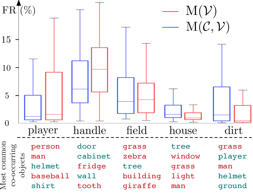
Figure 3: Boxplot representing the distribution of the correct ranks (First Relevant in $\%$) for five randomly selected classes of the target domain, with the context model $S_{L}\cup S_{H}\cup T_{L}$. Below are listed, by order of frequency, the classes that co-occur the most with the object of interest (classes of $\mathcal{T}$ in green; $\mathcal{S}$ in red).

To gain a deeper understanding of contextual information, we compare in Figure 3 the predictions of M$(\mathcal{V})$ and the global model M$(\mathcal{C},\mathcal{V})$. We randomly select five classes of the target domain and plot, for all instances of these classes in the test set of Visual Genome, the distribution of the predicted ranks of the correct class (in percentage); we also list the classes that appear the most in the context of these classes. We observe that, for certain classes (player, handle and field), contextual information helps to refine the predictions; for others (house and dirt), contextual information degrades the quality of the predictions.

First, we can outline that visual context can guide the model towards a more precise prediction. For example, a player, without context, could be categorized as person, man or woman; but visual context provides important complementary information (e.g, helmet, baseball) that grounds person in a sport setting, and thus suggests that the person could be playing. Visual context is also particularly relevant when the object of interest has a generic shape. For example, handle, without context, is visually similar to many round objects; but the presence of objects like door or fridge in the context helps determine the nature of the object of interest.

To get a better insight on the role of context, we cherry-picked examples where the visual or the prior component is inacurrate and the context component is able to counterbalance the final prediction (Figure 4). In (i), for example, the visual component ranks flower at position 223. However, the context component assesses flower to be highly probable in this context, due to the presence of source objects like vase, water, stems or grass, but also target objects like the other flowers around. At the inference phase, probabilities are aggregated and flower is ranked first.

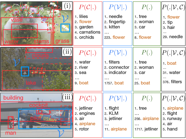
Figure 4: Qualitative examples where the global model M$(\mathcal{C}_{S_{L}\cup S_{H}\cup T_{L}},\mathcal{V})$ correctly retrieves the class ($\mathcal{T}$ classes only).

It is worth noting that our work is not without limitations. Indeed, some classes (such as house and dirt) have a wide range of possible contexts; in these cases, context is not a discriminating factor. This is confirmed by a complementary analysis: the Spearman correlation between the number of unique context objects and $\delta_{C}$, the relative gain of M$(\mathcal{C}_{S_{H}},\mathcal{V})$ over M$(\mathcal{V})$, is $\rho=-0.31$. In other terms, contextual information is useful for specific objects, which appear in particular contexts; for objects that are too generic, adding contextual information can be a source of noise.

6 Conclusion

In this paper, we introduced a new approach for ZSL: context-aware ZSL, along with a corresponding model, using complementary contextual information that significantly improves predictions. Possible extensions could include spatial features of objects, and, more importantly, removing the dependence on the detection of object boxes to make it fully applicable to real-world images (e.g. by using a Region Proposal Network (Ren et al., 2015)) Finally, designing grounded word embeddings that include more visual context information would also benefit such models.

Appendix A Additional negative results

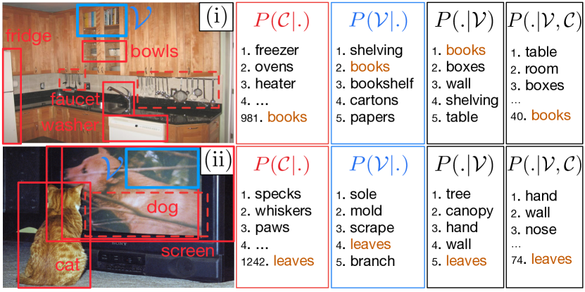
Figure 5: Qualitative analysis: negative examples where the use of the context leads to degraded predictions, i.e. examples where model M$(\mathcal{C}_{S_{L}\cup S_{H}\cup T_{L}},\mathcal{V})$ is worse than the simpler model M$(\mathcal{V})$ ($\mathcal{T}$ classes only).

As explained in Section 5.3, using contextual information can sometimes degrade predictions. We provide here additional examples, when an object occurs in an environment in which it is unexpected. For example, Figure 5 shows a picture of a kitchen where the object of interest to be predicted is “books”. Given only the surrounding environment, predicted objects are logically related to the environment of a kitchen (“freezer”, “oven”, …), and the correct label is badly ranked (because it is unexpected in such an environment). However, the model M$(\mathcal{V})$ retrieves the correct label, given only the region of interest. Finally, integrating contextual information in the final model M$(\mathcal{C}_{S_{L}\cup S_{H}\cup T_{L}},\mathcal{V})$ leads to worse performances over M$(\mathcal{V})$.

Appendix B Generalized ZSL

In the previous sections, retrieval in done only among classes of the domain of interest, this is the classical zero-shot learning setting. We now report results obtained when both source and target object classes exist in the retrieval space: this setting amounts to generalized zero-shot learning. Results are reported in Table 3.

Table 3: Evaluation of various information sources, with varying levels of supervision. Generalized ZSL setting. MFR scores in $\%$. $\delta_{C}$ is the relative improvement (in $\%$) of M$(\mathcal{C}_{S_{H}},\mathcal{V})$ over M$(\mathcal{V})$.

		Target domain $\mathcal{T}$			Source domain $\mathcal{S}$
	$p_{\text{sup}}$	10%	50%	90%	10%	50%	90%
	Domain size	4358	2421	484	484	2421	4358
Models	Random	100	100	100	100	100	100
	M$(\varnothing)$	39.6	26.3	16.9	6.6	8.68	10.9
	M$(\mathcal{V})$	21.0	11.8	6.9	0.9	2.3	3.5
	M$(\mathcal{C}_{S_{H}})$	28.6	15.0	10.7	3.5	3.9	4.4
	M$(\mathcal{C}_{S_{H}},\mathcal{V})$	18.2	9.4	6.0	0.8	1.8	2.4
	$\delta_{\mathcal{C}}$	13.4	20.2	13.4	13.8	24.4	31.5

Appendix C MRR and top-$k$ performances

ZSL models are usually evaluated with recall@$k$ or MRR (mearn reciprocal rank, i.e. harmonic mean). However, the metrics are not optimal to evaluate our models for two reasons:

• Theoretically, recent research points out that RR is not an interval scale and thus MRR should not be used (Fuhr, Some Common Mistakes In IR Evaluation, And How They Can Be Avoided. SIGIR Forum 2017 ; Ferrante et al. Are IR evaluation measures on an interval scale? ICTIR 2017).

• Practically, we make the size of the target domain vary (10%, 50%, 90%). MRR and top-$k$ scores cannot be compared across these scenarios (e.g. top-5 among 100 entities is not comparable to top-5 among 1000)

Therefore, as explained in Section 4.2 we used MFR (mean first relevant): the arithmetic mean of rank numbers (linearly rescaled to have 100% for random model and 0% for perfect model). FR is an interval scale and thus can be averaged.

However, we report here top$k$ and MRR scores in Table 4.

Table 4: Recall@$k$ ($k\in\{1,5,10\}$) (in percentage) and MRR scores (in percentage). $p_{\text{sup}}=50\%$.

	Target domain $\mathcal{T}$				Source domain $\mathcal{S}$
	Recall @			MRR	Recall @			MRR
	1	5	10		1	5	10
Random	<.1	0.2	0.4	<.1	<.1	0.2	0.4	<.1
M$(\varnothing)$	3.2	11.7	16.3	7.8	5.7	17.9	24.9	12.5
M$(\mathcal{V})$	14.7	33.5	43.2	24.0	36.3	63.8	73.1	48.8
M$(\mathcal{C}_{S_{H}})$	5.9	17.8	25.4	11.9	17.3	43.7	56.7	29.9
M$(\mathcal{C}_{S_{H}},\mathcal{V})$	15.0	34.7	44.7	24.7	41.6	70.6	78.6	54.2

References

- Akata et al. (2015) Akata, Z., Reed, S. E., Walter, D., Lee, H., and Schiele, B. Evaluation of output embeddings for fine-grained image classification. In IEEE Conference on Computer Vision and Pattern Recognition, CVPR 2015, Boston, MA, USA, June 7-12, 2015, pp. 2927–2936, 2015. doi: 10.1109/CVPR.2015.7298911. URL https://doi.org/10.1109/CVPR.2015.7298911.
- Akata et al. (2016) Akata, Z., Perronnin, F., Harchaoui, Z., and Schmid, C. Label-embedding for image classification. IEEE Trans. Pattern Anal. Mach. Intell., 38(7):1425–1438, 2016. doi: 10.1109/TPAMI.2015.2487986. URL https://doi.org/10.1109/TPAMI.2015.2487986.
- Ba et al. (2015) Ba, L. J., Swersky, K., Fidler, S., and Salakhutdinov, R. Predicting deep zero-shot convolutional neural networks using textual descriptions. In 2015 IEEE International Conference on Computer Vision, ICCV 2015, Santiago, Chile, December 7-13, 2015, pp. 4247–4255, 2015. doi: 10.1109/ICCV.2015.483. URL https://doi.org/10.1109/ICCV.2015.483.
- Bansal et al. (2018) Bansal, A., Sikka, K., Sharma, G., Chellappa, R., and Divakaran, A. Zero-shot object detection. In Computer Vision - ECCV 2018 - 15th European Conference, Munich, Germany, September 8-14, 2018, Proceedings, Part I, pp. 397–414, 2018. doi: 10.1007/978-3-030-01246-5“˙24. URL https://doi.org/10.1007/978-3-030-01246-5_24.
- Bell et al. (2016) Bell, S., Zitnick, C. L., Bala, K., and Girshick, R. B. Inside-outside net: Detecting objects in context with skip pooling and recurrent neural networks. In 2016 IEEE Conference on Computer Vision and Pattern Recognition, CVPR 2016, Las Vegas, NV, USA, June 27-30, 2016, pp. 2874–2883, 2016. doi: 10.1109/CVPR.2016.314. URL https://doi.org/10.1109/CVPR.2016.314.
- Bengio et al. (2013) Bengio, S., Dean, J., Erhan, D., Ie, E., Le, Q. V., Rabinovich, A., Shlens, J., and Singer, Y. Using web co-occurrence statistics for improving image categorization. CoRR, abs/1312.5697, 2013. URL http://arxiv.org/abs/1312.5697.
- Bucher et al. (2016) Bucher, M., Herbin, S., and Jurie, F. Improving semantic embedding consistency by metric learning for zero-shot classiffication. In Computer Vision - ECCV 2016 - 14th European Conference, Amsterdam, The Netherlands, October 11-14, 2016, Proceedings, Part V, pp. 730–746, 2016. doi: 10.1007/978-3-319-46454-1“˙44. URL https://doi.org/10.1007/978-3-319-46454-1_44.
- Chen et al. (2015) Chen, Q., Song, Z., Dong, J., Huang, Z., Hua, Y., and Yan, S. Contextualizing object detection and classification. IEEE Trans. Pattern Anal. Mach. Intell., 37(1):13–27, 2015. doi: 10.1109/TPAMI.2014.2343217. URL https://doi.org/10.1109/TPAMI.2014.2343217.
- Chen et al. (2018) Chen, X., Li, L., Fei-Fei, L., and Gupta, A. Iterative visual reasoning beyond convolutions. In 2018 IEEE Conference on Computer Vision and Pattern Recognition, CVPR 2018, Salt Lake City, UT, USA, June 18-22, 2018, pp. 7239–7248, 2018. doi: 10.1109/CVPR.2018.00756. URL http://openaccess.thecvf.com/content_cvpr_2018/html/Chen_Iterative_Visual_Reasoning_CVPR_2018_paper.html.
- Chu & Cai (2018) Chu, W. and Cai, D. Deep feature based contextual model for object detection. Neurocomputing, 275:1035–1042, 2018. doi: 10.1016/j.neucom.2017.09.048. URL https://doi.org/10.1016/j.neucom.2017.09.048.
- Deng et al. (2009a) Deng, J., Dong, W., Socher, R., Li, L., Li, K., and Li, F. Imagenet: A large-scale hierarchical image database. In 2009 IEEE Computer Society Conference on Computer Vision and Pattern Recognition (CVPR 2009), 20-25 June 2009, Miami, Florida, USA, pp. 248–255, 2009a. doi: 10.1109/CVPRW.2009.5206848. URL https://doi.org/10.1109/CVPRW.2009.5206848.
- Deng et al. (2009b) Deng, J., Dong, W., Socher, R., Li, L.-J., Li, K., and Fei-Fei, L. ImageNet: A Large-Scale Hierarchical Image Database. In CVPR09, 2009b.
- Farhadi et al. (2009a) Farhadi, A., Endres, I., Hoiem, D., and Forsyth, D. A. Describing objects by their attributes. In 2009 IEEE Computer Society Conference on Computer Vision and Pattern Recognition (CVPR 2009), 20-25 June 2009, Miami, Florida, USA, pp. 1778–1785, 2009a. doi: 10.1109/CVPRW.2009.5206772. URL https://doi.org/10.1109/CVPRW.2009.5206772.
- Farhadi et al. (2009b) Farhadi, A., Endres, I., Hoiem, D., and Forsyth, D. A. Describing objects by their attributes. In 2009 IEEE Computer Society Conference on Computer Vision and Pattern Recognition (CVPR 2009), 20-25 June 2009, Miami, Florida, USA, pp. 1778–1785, 2009b. doi: 10.1109/CVPRW.2009.5206772. URL https://doi.org/10.1109/CVPRW.2009.5206772.
- Ferrante et al. (2017) Ferrante, M., Ferro, N., and Pontarollo, S. Are IR evaluation measures on an interval scale? In Proceedings of the ACM SIGIR International Conference on Theory of Information Retrieval, ICTIR 2017, Amsterdam, The Netherlands, October 1-4, 2017, pp. 67–74, 2017. doi: 10.1145/3121050.3121058. URL https://doi.org/10.1145/3121050.3121058.
- Frome et al. (2013) Frome, A., Corrado, G. S., Shlens, J., Bengio, S., Dean, J., Ranzato, M., and Mikolov, T. Devise: A deep visual-semantic embedding model. In Advances in Neural Information Processing Systems 26: 27th Annual Conference on Neural Information Processing Systems 2013. Proceedings of a meeting held December 5-8, 2013, Lake Tahoe, Nevada, United States., pp. 2121–2129, 2013. URL http://papers.nips.cc/paper/5204-devise-a-deep-visual-semantic-embedding-model.
- Fu et al. (2014) Fu, Y., Hospedales, T. M., Xiang, T., and Gong, S. Learning multimodal latent attributes. IEEE Trans. Pattern Anal. Mach. Intell., 36(2):303–316, 2014. doi: 10.1109/TPAMI.2013.128. URL https://doi.org/10.1109/TPAMI.2013.128.
- Fu et al. (2015a) Fu, Y., Yang, Y., Hospedales, T. M., Xiang, T., and Gong, S. Transductive multi-label zero-shot learning. CoRR, abs/1503.07790, 2015a. URL http://arxiv.org/abs/1503.07790.
- Fu et al. (2015b) Fu, Z., Xiang, T. A., Kodirov, E., and Gong, S. Zero-shot object recognition by semantic manifold distance. In IEEE Conference on Computer Vision and Pattern Recognition, CVPR 2015, Boston, MA, USA, June 7-12, 2015, pp. 2635–2644, 2015b. doi: 10.1109/CVPR.2015.7298879. URL https://doi.org/10.1109/CVPR.2015.7298879.
- Fuhr (2017) Fuhr, N. Some common mistakes in IR evaluation, and how they can be avoided. SIGIR Forum, 51(3):32–41, 2017. doi: 10.1145/3190580.3190586. URL https://doi.org/10.1145/3190580.3190586.
- Galleguillos et al. (2008) Galleguillos, C., Rabinovich, A., and Belongie, S. J. Object categorization using co-occurrence, location and appearance. In 2008 IEEE Computer Society Conference on Computer Vision and Pattern Recognition (CVPR 2008), 24-26 June 2008, Anchorage, Alaska, USA, 2008. doi: 10.1109/CVPR.2008.4587799. URL https://doi.org/10.1109/CVPR.2008.4587799.
- Harris (1954) Harris, Z. S. Distributional structure. Word, 10(2-3):146–162, 1954.
- He et al. (2004) He, X., Zemel, R. S., and Carreira-Perpiñán, M. Á. Multiscale conditional random fields for image labeling. In 2004 IEEE Computer Society Conference on Computer Vision and Pattern Recognition (CVPR 2004), with CD-ROM, 27 June - 2 July 2004, Washington, DC, USA, pp. 695–702, 2004. doi: 10.1109/CVPR.2004.173. URL http://doi.ieeecomputersociety.org/10.1109/CVPR.2004.173.
- Kingma & Ba (2014) Kingma, D. P. and Ba, J. Adam: A method for stochastic optimization. CoRR, abs/1412.6980, 2014. URL http://arxiv.org/abs/1412.6980.
- Kodirov et al. (2017) Kodirov, E., Xiang, T., and Gong, S. Semantic autoencoder for zero-shot learning. In 2017 IEEE Conference on Computer Vision and Pattern Recognition, CVPR 2017, Honolulu, HI, USA, July 21-26, 2017, pp. 4447–4456, 2017. doi: 10.1109/CVPR.2017.473. URL https://doi.org/10.1109/CVPR.2017.473.
- Krishna et al. (2017) Krishna, R., Zhu, Y., Groth, O., Johnson, J., Hata, K., Kravitz, J., Chen, S., Kalantidis, Y., Li, L., Shamma, D. A., Bernstein, M. S., and Fei-Fei, L. Visual genome: Connecting language and vision using crowdsourced dense image annotations. International Journal of Computer Vision, 123(1):32–73, 2017. doi: 10.1007/s11263-016-0981-7. URL https://doi.org/10.1007/s11263-016-0981-7.
- Lampert et al. (2009) Lampert, C. H., Nickisch, H., and Harmeling, S. Learning to detect unseen object classes by between-class attribute transfer. In 2009 IEEE Computer Society Conference on Computer Vision and Pattern Recognition (CVPR 2009), 20-25 June 2009, Miami, Florida, USA, pp. 951–958, 2009. doi: 10.1109/CVPRW.2009.5206594. URL https://doi.org/10.1109/CVPRW.2009.5206594.
- Lampert et al. (2014) Lampert, C. H., Nickisch, H., and Harmeling, S. Attribute-based classification for zero-shot visual object categorization. IEEE Trans. Pattern Anal. Mach. Intell., 36(3):453–465, 2014. doi: 10.1109/TPAMI.2013.140. URL https://doi.org/10.1109/TPAMI.2013.140.
- Lecun et al. (1998) Lecun, Y., Bottou, L., Bengio, Y., and Haffner, P. Gradient-based learning applied to document recognition. In Proceedings of the IEEE, pp. 2278–2324, 1998.
- LeCun et al. (2006) LeCun, Y., Chopra, S., and Hadsell, R. A tutorial on energy-based learning. Predicting Structured Data, 1:0, 2006.
- Liu et al. (2011) Liu, J., Kuipers, B., and Savarese, S. Recognizing human actions by attributes. In The 24th IEEE Conference on Computer Vision and Pattern Recognition, CVPR 2011, Colorado Springs, CO, USA, 20-25 June 2011, pp. 3337–3344, 2011. doi: 10.1109/CVPR.2011.5995353. URL https://doi.org/10.1109/CVPR.2011.5995353.
- Long et al. (2017) Long, Y., Liu, L., Shao, L., Shen, F., Ding, G., and Han, J. From zero-shot learning to conventional supervised classification: Unseen visual data synthesis. In 2017 IEEE Conference on Computer Vision and Pattern Recognition, CVPR 2017, Honolulu, HI, USA, July 21-26, 2017, pp. 6165–6174, 2017. doi: 10.1109/CVPR.2017.653. URL https://doi.org/10.1109/CVPR.2017.653.
- Lu et al. (2016) Lu, C., Krishna, R., Bernstein, M. S., and Li, F. Visual relationship detection with language priors. In Computer Vision - ECCV 2016 - 14th European Conference, Amsterdam, The Netherlands, October 11-14, 2016, Proceedings, Part I, pp. 852–869, 2016. doi: 10.1007/978-3-319-46448-0“˙51. URL https://doi.org/10.1007/978-3-319-46448-0_51.
- Mensink et al. (2012) Mensink, T., Verbeek, J. J., Perronnin, F., and Csurka, G. Metric learning for large scale image classification: Generalizing to new classes at near-zero cost. In Computer Vision - ECCV 2012 - 12th European Conference on Computer Vision, Florence, Italy, October 7-13, 2012, Proceedings, Part II, pp. 488–501, 2012. doi: 10.1007/978-3-642-33709-3“˙35. URL https://doi.org/10.1007/978-3-642-33709-3_35.
- Mensink et al. (2014) Mensink, T., Gavves, E., and Snoek, C. Costa: Co-occurrence statistics for zero-shot classification. 2014 IEEE Conference on Computer Vision and Pattern Recognition, pp. 2441–2448, 2014.
- Mikolov et al. (2013) Mikolov, T., Sutskever, I., Chen, K., Corrado, G. S., and Dean, J. Distributed representations of words and phrases and their compositionality. In Advances in Neural Information Processing Systems 26: 27th Annual Conference on Neural Information Processing Systems 2013. Proceedings of a meeting held December 5-8, 2013, Lake Tahoe, Nevada, United States., pp. 3111–3119, 2013. URL http://papers.nips.cc/paper/5021-distributed-representations-of-words-and-phrases-and-their-compositionality.
- Norouzi et al. (2013) Norouzi, M., Mikolov, T., Bengio, S., Singer, Y., Shlens, J., Frome, A., Corrado, G., and Dean, J. Zero-shot learning by convex combination of semantic embeddings. CoRR, abs/1312.5650, 2013. URL http://arxiv.org/abs/1312.5650.
- Palatucci et al. (2009) Palatucci, M., Pomerleau, D., Hinton, G. E., and Mitchell, T. M. Zero-shot learning with semantic output codes. In Advances in Neural Information Processing Systems 22: 23rd Annual Conference on Neural Information Processing Systems 2009. Proceedings of a meeting held 7-10 December 2009, Vancouver, British Columbia, Canada., pp. 1410–1418, 2009. URL http://papers.nips.cc/paper/3650-zero-shot-learning-with-semantic-output-codes.
- Parikh & Grauman (2011) Parikh, D. and Grauman, K. Interactively building a discriminative vocabulary of nameable attributes. In The 24th IEEE Conference on Computer Vision and Pattern Recognition, CVPR 2011, Colorado Springs, CO, USA, 20-25 June 2011, pp. 1681–1688, 2011. doi: 10.1109/CVPR.2011.5995451. URL https://doi.org/10.1109/CVPR.2011.5995451.
- Pelletier (2001) Pelletier, F. J. Did frege believe frege’s principle? Journal of Logic, Language and information, 10(1):87–114, 2001.
- Pennington et al. (2014) Pennington, J., Socher, R., and Manning, C. D. Glove: Global vectors for word representation. In Proceedings of the 2014 Conference on Empirical Methods in Natural Language Processing, EMNLP 2014, October 25-29, 2014, Doha, Qatar, A meeting of SIGDAT, a Special Interest Group of the ACL, pp. 1532–1543, 2014. URL http://aclweb.org/anthology/D/D14/D14-1162.pdf.
- Peters et al. (2018) Peters, M. E., Neumann, M., Iyyer, M., Gardner, M., Clark, C., Lee, K., and Zettlemoyer, L. Deep contextualized word representations. In Proceedings of the 2018 Conference of the North American Chapter of the Association for Computational Linguistics: Human Language Technologies, NAACL-HLT 2018, New Orleans, Louisiana, USA, June 1-6, 2018, Volume 1 (Long Papers), pp. 2227–2237, 2018.
- Qiao et al. (2016) Qiao, R., Liu, L., Shen, C., and van den Hengel, A. Less is more: Zero-shot learning from online textual documents with noise suppression. In 2016 IEEE Conference on Computer Vision and Pattern Recognition, CVPR 2016, Las Vegas, NV, USA, June 27-30, 2016, pp. 2249–2257, 2016. doi: 10.1109/CVPR.2016.247. URL https://doi.org/10.1109/CVPR.2016.247.
- Rabinovich et al. (2007) Rabinovich, A., Vedaldi, A., Galleguillos, C., Wiewiora, E., and Belongie, S. J. Objects in context. In IEEE 11th International Conference on Computer Vision, ICCV 2007, Rio de Janeiro, Brazil, October 14-20, 2007, pp. 1–8, 2007. doi: 10.1109/ICCV.2007.4408986. URL https://doi.org/10.1109/ICCV.2007.4408986.
- Real et al. (2018) Real, E., Aggarwal, A., Huang, Y., and Le, Q. V. Regularized evolution for image classifier architecture search. CoRR, abs/1802.01548, 2018. URL http://arxiv.org/abs/1802.01548.
- Ren et al. (2015) Ren, S., He, K., Girshick, R. B., and Sun, J. Faster R-CNN: towards real-time object detection with region proposal networks. In Advances in Neural Information Processing Systems 28: Annual Conference on Neural Information Processing Systems 2015, December 7-12, 2015, Montreal, Quebec, Canada, pp. 91–99, 2015. URL http://papers.nips.cc/paper/5638-faster-r-cnn-towards-real-time-object-detection-with-region-proposal-networks.
- Romera-Paredes & Torr (2015) Romera-Paredes, B. and Torr, P. H. S. An embarrassingly simple approach to zero-shot learning. In Proceedings of the 32nd International Conference on Machine Learning, ICML 2015, Lille, France, 6-11 July 2015, pp. 2152–2161, 2015. URL http://jmlr.org/proceedings/papers/v37/romera-paredes15.html.
- Schakel & Wilson (2015) Schakel, A. M. J. and Wilson, B. J. Measuring word significance using distributed representations of words. CoRR, abs/1508.02297, 2015. URL http://arxiv.org/abs/1508.02297.
- Szegedy et al. (2016) Szegedy, C., Vanhoucke, V., Ioffe, S., Shlens, J., and Wojna, Z. Rethinking the inception architecture for computer vision. In 2016 IEEE Conference on Computer Vision and Pattern Recognition, CVPR 2016, Las Vegas, NV, USA, June 27-30, 2016, pp. 2818–2826, 2016. doi: 10.1109/CVPR.2016.308. URL https://doi.org/10.1109/CVPR.2016.308.
- Torralba (2003) Torralba, A. Contextual priming for object detection. International Journal of Computer Vision, 53(2):169–191, 2003. doi: 10.1023/A:1023052124951. URL https://doi.org/10.1023/A:1023052124951.
- Torralba et al. (2010) Torralba, A., Murphy, K. P., and Freeman, W. T. Using the forest to see the trees: exploiting context for visual object detection and localization. Commun. ACM, 53(3):107–114, 2010. doi: 10.1145/1666420.1666446. URL http://doi.acm.org/10.1145/1666420.1666446.
- Wah et al. (2011) Wah, C., Branson, S., Welinder, P., Perona, P., and Belongie, S. The caltech-ucsd birds-200-2011 dataset. 2011.
- Weston et al. (2011) Weston, J., Bengio, S., and Usunier, N. WSABIE: scaling up to large vocabulary image annotation. In IJCAI 2011, Proceedings of the 22nd International Joint Conference on Artificial Intelligence, Barcelona, Catalonia, Spain, July 16-22, 2011, pp. 2764–2770, 2011. doi: 10.5591/978-1-57735-516-8/IJCAI11-460. URL https://doi.org/10.5591/978-1-57735-516-8/IJCAI11-460.
- Wolf & Bileschi (2006) Wolf, L. and Bileschi, S. M. A critical view of context. International Journal of Computer Vision, 69(2):251–261, 2006. doi: 10.1007/s11263-006-7538-0. URL https://doi.org/10.1007/s11263-006-7538-0.
- Xian et al. (2016) Xian, Y., Akata, Z., Sharma, G., Nguyen, Q. N., Hein, M., and Schiele, B. Latent embeddings for zero-shot classification. In 2016 IEEE Conference on Computer Vision and Pattern Recognition, CVPR 2016, Las Vegas, NV, USA, June 27-30, 2016, pp. 69–77, 2016. doi: 10.1109/CVPR.2016.15. URL https://doi.org/10.1109/CVPR.2016.15.
- Yang et al. (2018) Yang, J., Lu, J., Lee, S., Batra, D., and Parikh, D. Graph R-CNN for scene graph generation. In Computer Vision - ECCV 2018 - 15th European Conference, Munich, Germany, September 8-14, 2018, Proceedings, Part I, pp. 690–706, 2018. doi: 10.1007/978-3-030-01246-5“˙41. URL https://doi.org/10.1007/978-3-030-01246-5_41.
- Yu et al. (2016) Yu, R., Chen, X., Morariu, V. I., and Davis, L. S. The role of context selection in object detection. In Proceedings of the British Machine Vision Conference 2016, BMVC 2016, York, UK, September 19-22, 2016, 2016. URL http://www.bmva.org/bmvc/2016/papers/paper133/index.html.
- Zablocki et al. (2018) Zablocki, É., Piwowarski, B., Soulier, L., and Gallinari, P. Learning Multi-Modal Word Representation Grounded in Visual Context. In Association for the Advancement of Artificial Intelligence (AAAI), New Orleans, United States, February 2018. URL https://hal.archives-ouvertes.fr/hal-01632414.
- Zellers et al. (2018) Zellers, R., Yatskar, M., Thomson, S., and Choi, Y. Neural motifs: Scene graph parsing with global context. In 2018 IEEE Conference on Computer Vision and Pattern Recognition, CVPR 2018, Salt Lake City, UT, USA, June 18-22, 2018, pp. 5831–5840, 2018. doi: 10.1109/CVPR.2018.00611. URL http://openaccess.thecvf.com/content_cvpr_2018/html/Zellers_Neural_Motifs_Scene_CVPR_2018_paper.html.
- Zhang et al. (2018) Zhang, H., Dana, K. J., Shi, J., Zhang, Z., Wang, X., Tyagi, A., and Agrawal, A. Context encoding for semantic segmentation. In 2018 IEEE Conference on Computer Vision and Pattern Recognition, CVPR 2018, Salt Lake City, UT, USA, June 18-22, 2018, pp. 7151–7160, 2018. doi: 10.1109/CVPR.2018.00747. URL http://openaccess.thecvf.com/content_cvpr_2018/html/Zhang_Context_Encoding_for_CVPR_2018_paper.html.
- Zhao et al. (2018) Zhao, B., Chang, B., Jie, Z., and Sigal, L. Modular generative adversarial networks. CoRR, abs/1804.03343, 2018. URL http://arxiv.org/abs/1804.03343.
- Zoph et al. (2017) Zoph, B., Vasudevan, V., Shlens, J., and Le, Q. V. Learning transferable architectures for scalable image recognition. CoRR, abs/1707.07012, 2017. URL http://arxiv.org/abs/1707.07012.