Table understanding in structured documents

Abstract

Table detection and extraction has been studied in the context of documents like reports, where tables are clearly outlined and stand out from the document structure visually. We study this topic in a rather more challenging domain of layout-heavy business documents, particularly invoices. Invoices present the novel challenges of tables being often without outlines - either in the form of borders or surrounding text flow - with ragged columns and widely varying data content. We will also show, that we can extract specific information from structurally different tables or table-like structures with one model. We present a comprehensive representation of a page using graph over word boxes, positional embeddings, trainable textual features and rephrase the table detection as a text box labeling problem. We will work on our newly presented dataset of pro forma invoices, invoices and debit note documents using this representation and propose multiple baselines to solve this labeling problem. We then propose a novel neural network model that achieves strong, practical results on the presented dataset and analyze the model performance and effects of graph convolutions and self-attention in detail.

I Introduction

Table detection and table extraction problems were already introduced in a competition ICDAR 2013, where the goal was to detect tables and extract cell structures from a dataset of mostly scientific documents [1]. Table can be defined as a set of content cells organized in a self-describing manner into such a structure, that groups cells into rows and columns. This was reflected in the metric defined in the competition, that scores tables based on the relations successfully extracted. Similarly, structured documents do have a self-describing structure, that often looks table-like.

We have decided to investigate the problem on business documents such as invoices, pro forma invoices and debit notes (referred for simplicity as invoices or invoice-type documents later in this text), where the aim is different. Namely - even table detection needs to be thought of in the context of document understanding, because invoices are inherently documents with textual information structured into more tables. Graphical borders and edges are sometimes present, however, they cannot be used for detection, because there is no general layout and very often there are no borders at all. Another obstacle for traditional methods is the fact, that the data can span over multiple lines of text which holds true also for the table cells.

Moreover, we require our model to ’understand’ the document in a way that it could classify tables and tabular structures based on their content. In practice the goal is to detect the whole table with the so-called ’line-items’ (detailed items of the total amount to pay) and, at the same time, extract only a specific information from the other tables (to find a ’field’). Simply said, not every table inside an invoice should be detected and reported as whole (see example invoice on figure 1). Usually in commercial applications this problem is tackled using a layout system that detects the layout and extracts the table (or a field) from a position where it usually happens to be; or employing another classification module, which selects the right table from several proposals. That increases the number of modules in the architecture and requires manual layout setups, while our goal is to have a trainable system that could leverage the commonalities present in the data without ongoing human support. To verify that, we will ensure that proper generalization of models predictions is evaluated on new layouts.

II Previous Work

The plethora of methods that have been previously used for the task is hard to summarize or compare since all the algorithms have been used/evaluated on different datasets and each have their strengths, weak spots and quirks. However, we found none of them well suited for working with structured documents (like invoices), since they in general have no fixed layout, language, captions, delimiters, fonts… For example, invoices vary in countries, companies and departments and changes in time. In order to retrieve any information from a structured document, you need to understand it.

In literature there are examples of table detection using heuristics [2], using layouts [3], regular expressions [4], or leveraging the presence of lines in tables [5, 6, 7, 8], or using clustering [9]. A great survey can be found in [10].

Tables were searched for also in HTML [11, 12], free text [13] or scientific articles with a method based on matching captions with content [14].

Machine learning methods and deep neural networks were also employed in several papers. The work [15] aims at scientific documents using fine tailored methods stacked atop each other. Reference [16] uses Fast R-CNN architecture with a novel idea of Euclidean distance feature to detect tables (which was compared to Tesseract). Reference [17] also uses (pretrained) Fast R-CNN and FCN semantic segmentation model for table extraction problem. In [8] work has been done on detection problem bottom up using the Hough transform, and extraction was solved with Markov networks and features from the cell positions. Reference [18] uses convolutions over the number (and sizes) of spaces in a line. A deep CNN approach was being investigated in [19], which combined CNNs for detecting row and columns, dilated convolutions, CRFs and saliency maps, they have also developed a webcrawler to extend their dataset. We tried and failed to get working results using the YOLO architecture [20] with textual datasets. (We have experimented with YOLO because some works aimed at table detection do use the family of R-CNNs, Fast R-CNNs and Mask R-CNNs, that preceded the development of YOLO.)

For document understanding, a graph representation of a document was examined in [21, 22], finding similar documents and reusing their goldstandards was done in [23].

III Methodology

We would like to define our target as creating a model for tabular or structured data understanding with relevant information detection and classification. The basic unit of information will be a word in a document’s page with its placement and possibly other features such as style (see PDF format text data organization [24] for example). In this text, we will be calling them simply as wordboxes.

With table understanding we mean a joint task of line-item table detection and information extraction from other tables. The information to be extracted is defined by the document use-case or semantics, for line-item table it is the whole table (’table detection’ task as defined in [1]), while for other structures it is just a specific infomation (’information extraction’ task). No other constraints apply, i.e. the data can span over multiple lines. So the model is required to understand a type of table internally and we hope, that the two tasks will boost the learning process for each other.

With line-item table detection method, we will understand a model, that could classify each wordbox in a document as being a part of a line-item content or not (which basically identifies the table itself, because all line-items tables happen to be well separated, so no instance segmentation is needed). Same classification approach will be used for other classes representing other types of content. The classes are acquired from expert annotations and, as it turns out, we are dealing with a multilabel problem, i.e. 35 classes in total, examples being the total amount or recipient address. Also, not every document contains instances of every class.

III-A Metrics and evaluation

We will observe the scores at validation and test splits, the test being composed not only of different data, but also of different layouts and invoice types, thus allowing us to observe the system scalability. The scores are:

• $F_{1}$ scores on line-item wordbox classification averaged from both positive classes and negative classes.
  At [1] a content oriented metric was defined for table detection on character level - each character being either in the table or out of the table. For us the basic unit is a wordbox, hence we will define our metric similarily to be the $F_{1}$ score of table body wordbox class classification.

• For other classes we will be looking at micro $F_{1}$ scores (only from positive classes, because the counts of positive samples are outnumbered by the negative samples - in total, the dataset contains $1.2\,\%$ positive classes).

We chose micro metric aggregation rule, because it gives higher importance to bigger documents (in the number of wordboxes) which we consider being more difficult for both human and machine.

We present our research as a novel approach, because referenced papers or commercial solutions cannot be customized to fit our aim. So we will compare only against baseline logistic regression over the model features.

III-B The data and their acquisition process

The data were acquired as a result of work of annotation and review teams together with automated preprocessing and error-finding algorithms, that reported errors in nearly $3\,\%$ of the annotation labels. Classes were annotated in our annotation apps by drawing a rectangle over the area with the target text. Manual inspection has revealed, that the annotations can erroneously overlap portions of neighbouring words, so for ground truth generation we have decided to select only the wordboxes that are being overlapped by the annotation rectangle by more than $20\,\%$ of their area.

Datasets

We have a dataset with $3554$ PDF invoice files consisting of $4848$ pages in total. The documents are of various vendors, layouts and languages, annotated with line-item table header and table body together with other structural information. And we also have a bigger dataset of $25071$ PDF files of $35880$ pages with just structural information without line-items (datasets are noted as ’small’ and ’big’ in the results).

The documents are standard PDF files, not scanned documents or documents captured by a digital camera. This decision will not impact the robustness of our model - given a process to extract bounding boxes and text, we can use our method in a straightforward manner.

Validation split is chosen to be 1/4 the size. The validation set measures adaptation, because it could contain similar invoice types from similar vendors. So in addition, we have created another testing set of $83$ documents, that have different invoice layouts and types to those in the training set to measure generalization.

Since this newly compiled dataset was never explored and made accessible before, we have published an anonymized version of the small dataset, that contains only the positions and sizes of wordboxes and annotations, no picture information and no readable text information – only a subset of some textual features. The dataset is to be found at https://github.com/rossumai/flying-rectangles

III-C Our approach

We want to operate based on the principle of reflecting the structure of the data in the model’s architecture, as Machine learning algorithms tend to perform better that way.

What will be the structured information at the input? The number of wordboxes per page can vary and so we have decided to perceive the input as an ordered sequence (see below).

In addition we will teach the network to not only detect line-item table in general, but also to detect a header in the table, because that could provide a meaningful information - the headers are always different from the contents.

The features of each wordbox are:

• Geometrical:

  • By geometrical algorithms we can construct a neighbourhood graph over the boxes, which can then be used by a graph CNN if we bound the number of neighbours on each edge of the box by a constant.
    Neighbours are generated for each wordbox ($W$) as follows - every other box is assigned to an edge of $W$, that has it in its field of view (being fair $90\text{\textdegree}$), then the closest (center to center Euclidian distance) $n$ neighbours are chosen for that edge. For example with $n=1$ see figure 1. The relation does not need to be symmetrical, but when higher number of closest neighbours will be used, the sets would have bigger overlap.

  • We can define a ’reading order of wordboxes’. In particular, based on the idea that if two boxes do overlap in a projection to $y$ axis by more than a given threshold, set to $50\,\%$ in our experiments, they should be regarded to be in the same line for a human reader. This not only defines an order of the boxes in which they will be given as sequence to the network, but also assigns a line number and order-in-line number to each box. To get more information, we can run this algorithm again on a $90\text{\textdegree}$ rotated version of the document. These integers are then subject to a positional embedding. Note, that the exact ordering/reading direction (left to right and top to bottom or vice versa) should not matter in the neural network design, thus giving us the freedom to process any language.

  • Each box has 4 normalized coordinates (left, top, right, bottom) that should be presented to the network also by positional embedding.

• Textual:

  • Each word can be presented using any fixed size representation, in our case we will use tailored features common in other NLP tasks (e.g. authorship attribution [25], named entity recognition [26], and sentiment analysis [27]). The features per wordbox are the counts of all characters, the counts of first two and last two characters, length of a word, number of uppercase and lowercase letters, number of text characters and number of digits. And finally, if the word is in fact a number, then the number scaled and cropped against different scales, zeroes for other text. The reason behind these features is that in an invoice there would be a larger number of named entities, ids and numbers, which are not easily embedded.

  • Trainable word features are employed as well, using convolutional architecture over sequence of one hot encoded, deaccented, lowercase characters (only alphabet, numeric characters and special characters “ ,.-+:/%?$£€#()&”’, all others are discarded).

• Image features:

  • Each wordbox has its corresponding crop in the original PDF file, where it is rendered using some font settings and also background, which could be crucial to line-item table (or header) detection, if it contains lines, for example, or different background color or gradient. So the network receives a crop from the original image, offsetted outwards to be bigger than the text area to see also the surroundings.

Each presented feature can be augmented, we have decided to do a random $1\,\%$ percent perturbation on coordinates and textual features representation.

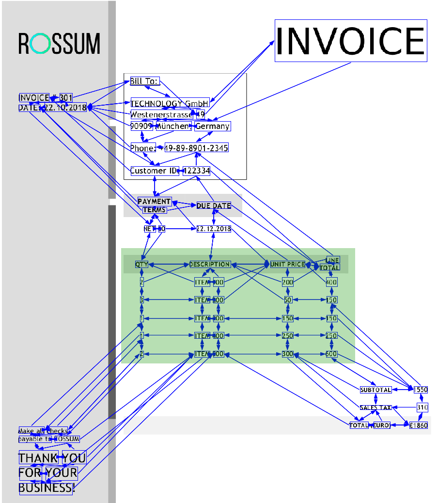
Figure 1: Sample invoice with edges defining neighbourhood wordboxes. Only the closest neighbour is connected for each wordbox. Green area is the line-item table. Note that above it lies a smaller table of payment terms and due date, from which only some information should be extracted and the table should not be reported. This invoice is artificially created for presentation and does not represent the invoices in our dataset.

III-D The architecture

As can be seen in Figure 2 and as we have stated before, the model uses 5 inputs - downsampled picture of the whole document ($620\times 877$), grayscaled; features of the wordboxes, including their boundingbox coordinates; on-hot characters with 40 one-hot encoded characters per each wordbox; neighbour ids - integers that define the neighbouring wordboxes on each side of the wordbox; and finally integer positions of each field defined by the geometrical ordering.

The positions are embedded by positional embeddings (defined and used in [28, 29], we use embedding size equal to 4 dimensions for $sin$ and 4 for $cos$, with divisor constant being $10000$) and then concatenated with other field features.

The picture is reduced by classical stacked convolution and maxpooling approach and then from its inner representation, field coordinates (left, top, right, bottom) are used to get a crop of a slightly bigger area (using morphological dilation) which is then appended to the field. Finally we have decided to give the model a grasp of the image as whole - a connection to the whole image flattened and then processed to 32 float features, which are also appended to each field’s features.

Before attention, dense, or graph convolution layers are used, all the input features are concatenated.

Our implementation of the graph convolution mechanism gathers features from the neighbouring wordboxes, concatenates them and feeds into a Dense layer. To note, our graph has a regularity that allows us to simplify the graph convolution - there does exist an upper bound on the number of edges for each node, so we do not need to use any general form graph convolutions as in [30, 31].

We have also employed a convolution layer over the ordering dimension (called convolution over sequence later in this text).

The rest of the network handles images and crops. The final output branch has an attention transformer module (from [28]) to be able to compare pairwise all the fields in hope that denser and regular areas (of texts in a table grid) can be detected better. Our attention transformer unit does not use causality, nor query masking and has 64 units and 8 heads.

Finally, the output is a multilabel problem, so sigmoidal layers are deployed together with binary crossentropy as the loss function.

The optimizer was chosen to be Adam. Model selected in each experimental run was always the one that performed best on the validation set (of the small dataset) in terms of loss, while the patience constant was $10$ epochs. Batched data were padded by zeros per batch (with zero sample weights). Class weights in our multi-task classification problem were chosen based on positive class occurrences. The network has $867k$ trainable parameters in total.

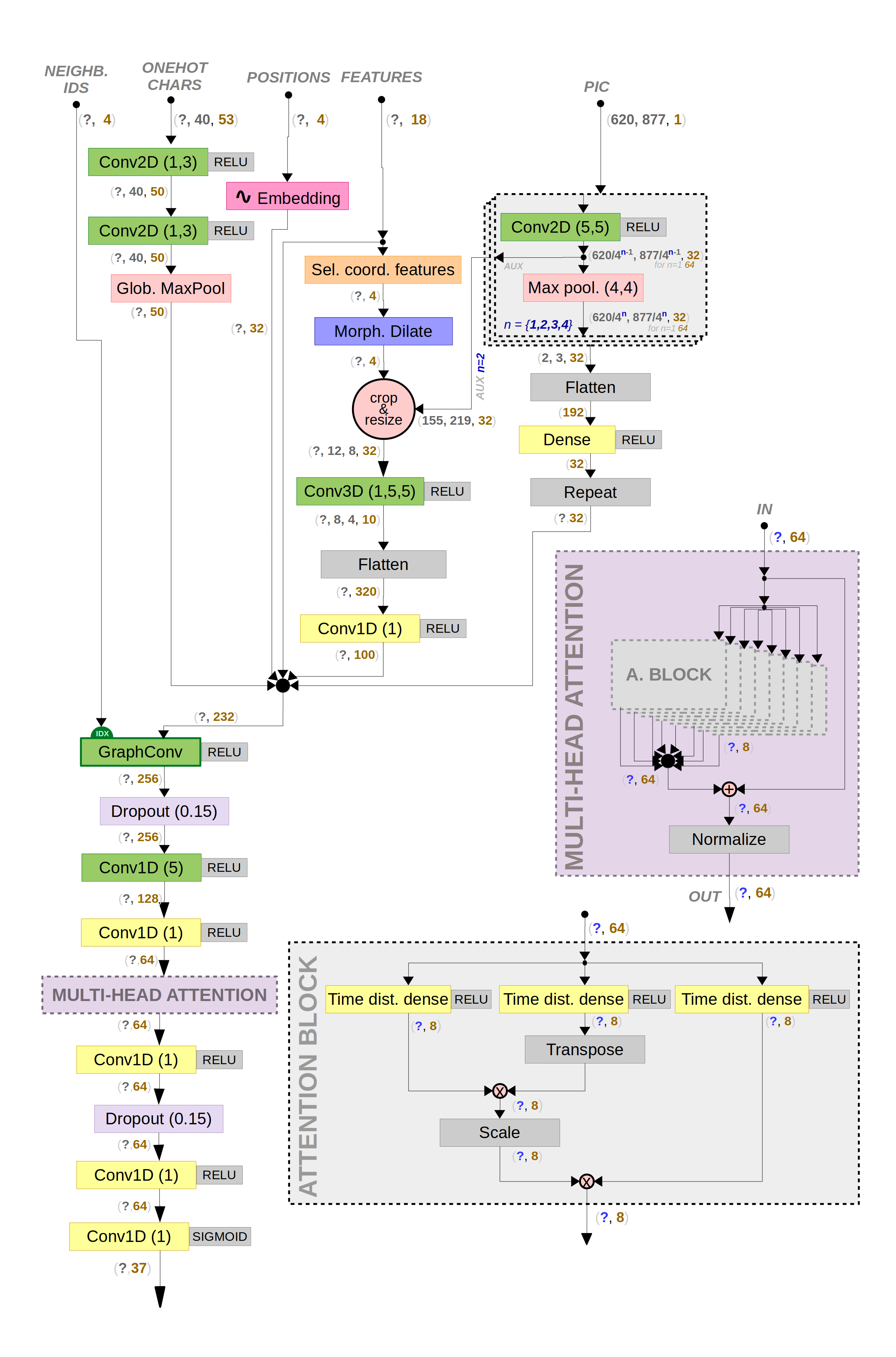
Figure 2: The model architecture. All features are concatenated together before the self attention mechanism and final layers. The cropping of the picture, embeddings and graph convolution all happen inside the network. Note that $Conv1D(1)$ can be also called a time distributed dense layer.

IV Experiments

The approach was tested on different data settings and different architectures. There are 4 groups of experiments:

1. Comparing logistic regression baseline against the neural network.
   To note, logistic regression baselines use all the inputs except the picture and trainable word embeddings. To inspect the importance of neighbouring boxes, we have compared the baseline without neighbours and the baseline with included information about one or more neighbours at each side (if present).

2. The importance and effect of each block of layers and each input and other parameters.
   The choice of modules to test was ’convolution with dropout after attention’ to test the dropout layer, ’convolution over sequence’ for the importance of input ordering and attention. Experiments dropping the graph convolution were done in variation of neighbours. Experiments on anonymized dataset fall also into this category. We have also tested the focal loss function [32], note that we do not vary final activations in our experiments here and use only sigmoidal, because they had best performance in earlier development process.

3. Specialization on a task where only line-items were classified and specialization on a task with all but line-items.

4. Evaluating the model’s adaptation performance on the big dataset (without line-items).

We will not be optimizing the number of neurons in the layers. The training was done on a single GPU and ran approximately in $23$ epochs for $5$ hours per experiment on small dataset.

IV-A Results

Table I summarizes experiments comparing the model against the logistic regression baseline, both with varying number of neighbours (more than $2$ not shown, because the results were not improving with the number of neighbours). The logistic regression baselines did improve with more neighbours, but failed to generalize. We can notice the big difference between line-item table detection and other classes coming from a possible observation that sometimes the table is the biggest one. The results also do reflect the nature of a specialized structured document, which invoices indeed are - to classify all the structured information is not easy for a person not working with invoices.

On the other hand, the optimal number of neighbours for the final architecture was 1, but we can notice, that 2 neighbours do help line-item table body detections. We have designed the algorithm with more than one neighbour in mind (with a single neighbour, the relation is not symmetrical), so other positional features are possibly being exploited more efficiently.

Table II shows, that the multihead attention module helps with generalization to unseen layouts, omitting the module makes the network prioritize adaptation on already seen layouts. Also without attention, the number of training epochs was twice (27) as much as with attention (13). Focal loss, prioritizing rare classes, does help line-item header detection, but is a cause for the decrease of the nonline-item score micro metric, as rare classes contribute less.

The importance of the convolutional layer over the sequence might come from our initial guess that this would give more importance to beginnings and endings of lines of words.

Table III compares different inputs and dataset choices. Although the architecture was optimized on the small dataset, the results imply that the model has the capacity to adapt and generalize also on bigger datasets. Looking at the anonymized version of datasets, without some inputs, it can be concluded that the network can learn to detect tight areas of evenly spaced words, being the line-item table. Also even base text features help the model generalize well. Overall the score on anonymized dataset means that the positional information is passed correctly and embedded in a right way for the network.

In table IV there can be seen that the tasks of finding line-items and other structural information do boost each other, with one exception being the header detection - it does help adaptation, but when omitted, the generalization score is higher.

The architecture provided on Figure 2 is the ’complete model’, that uses binary crossentropy, all inputs and all modules and a single neighbour at each side of each box. Its generalization performance on unseen invoice types was $93\,\%$ on detecting line-items and $66\,\%$ for other classes ($87\,\%$ on similar layouts). To verify what the line-item detection scores mean in practice, we have run the prediction on the sample invoices (Figure 1), where our algorithm correctly detected the line-item table up to 2 false positive words, which are easily filtered out (heuristic filtering results are not reported).

TABLE I:

Experiments against the baseline	Adaptation			Generalization
	line-items		others	line-items		others
	body $F_{1}$	header $F_{1}$	micro $F_{1}$	body $F_{1}$	header $F_{1}$	micro $F_{1}$
complete model (without neighbours)	0.9666	0.9969	0.8687	0.9242	0.9876	0.6609
complete model (1 neighbour)	0.9738	0.9967	0.8790	0.9389	0.9864	0.6650
complete model (with 2 neighbours)	0.9762	0.9963	0.8749	0.9408	0.9860	0.6629
logistic regression without neighbours	0.7594	0.9477	0.0004	0.7560	0.9362	0.0000
logistic regression with 1 neighbour	0.8664	0.9663	0.1482	0.8071	0.9461	0.0327
logistic regression with 2 neighbours	0.8939	0.9724	0.2276	0.8284	0.9493	0.0525

TABLE II:

Experiments with ablation	Adaptation			Generalization
	line-items		others	line-items		others
	body $F_{1}$	header $F_{1}$	micro $F_{1}$	body $F_{1}$	header $F_{1}$	micro $F_{1}$
complete model	0.9738	0.9967	0.8790	0.9389	0.9864	0.6650
focal loss	0.9735	0.9969	0.8557	0.9383	0.9878	0.6398
no convolution over sequence	0.9670	0.9945	0.8638	0.9101	0.9800	0.6237
no attention	0.9780	0.9967	0.8806	0.9348	0.9864	0.6487
no convolution with dropout after attention	0.9646	0.9950	0.8435	0.9168	0.9807	0.6050

TABLE III:

Experiments with inputs variations	dataset	Adaptation			Generalization
		line-items		others	line-items		others
		body $F_{1}$	header $F_{1}$	micro $F_{1}$	body $F_{1}$	header $F_{1}$	micro $F_{1}$
complete model (all inputs)	small	0.9738	0.9967	0.8790	0.9389	0.9864	0.6650
no text embeddings	small	0.9702	0.9921	0.7772	0.9108	0.9771	0.5118
no picture, only some text features	anonym	0.9694	0.9943	0.4518	0.9185	0.9805	0.4745
no picture, no text features	anonym	0.9588	0.9848	0.6836	0.8919	0.9549	0.2152
complete model (all inputs)	big	N/A	N/A	0.8487	N/A	N/A	N/A

TABLE IV:

Experiments with training target variations	dataset	Adaptation			Generalization
		line-items		others	line-items		others
		body $F_{1}$	header $F_{1}$	micro $F_{1}$	body $F_{1}$	header $F_{1}$	micro $F_{1}$
complete model (all outputs)	small	0.9738	0.9967	0.8790	0.9389	0.9864	0.6650
only line-items	small	0.9027	0.9950	N/A	0.8762	0.9766	N/A
no line-item header	small	0.9736	N/A	0.8777	0.9394	N/A	0.6731
all but line-items	small	N/A	N/A	0.8632	N/A	N/A	0.6247
complete model (other than line-items targets)	big	N/A	N/A	0.8487	N/A	N/A	N/A

V Conclusions

We have found a fully trainable method for table detection and content understanding in structured documents, that is able to detect a specific line-item table and extract only some information from other tables even in the presence of imbalanced classes and multiple layouts, languages and invoice types. Anonymized version of our dataset was published, as no similar dataset has been publicly available to date.

Trying to detect line-item headers in a single model did lead the model to underperform, with a hint to use focal loss for such task. Also, we have discovered, that attention module was important to generalization for new invoice types, while using only close neighbours did lead to better adaptation on already seen layouts.

The system’s ability to correctly scale to completely new invoice types is successfully verified for the line-item table detection task at 93% and measured to be 66% on 35 ’other’ classes.

Future work can include line-item table extractions, architecture and hyperparameter tuning for bigger datasets, experiments with the usage of different text features or embeddings and image augmentations. It could be also measured how many annotations are needed for the ’other’ classes to adapt onto new invoice types.

Acknowlegment

The work was supported by the grant SVV-2017-260455. We would also like to thank to the annotation team and the rest of the research team.

Replace this box by an image with a width of 1 in and a height of 1.25 in!

Your Name

Coauthor Same again for the co-author, but without photo

References

- [1] M. Göbel, T. Hassan, E. Oro, and G. Orsi, “Icdar 2013 table competition,” in Document Analysis and Recognition (ICDAR), 2013 12th International Conference on. IEEE, 2013, pp. 1449–1453.
- [2] A. Jahan Mac and R. G. Ragel, “Locating Tables in Scanned Documents for Reconstructing and Republishing (ICIAfS14),” arXiv e-prints, p. arXiv:1412.7689, Dec. 2014.
- [3] T. Dhiran and R. Sharma, “Table detection and extraction from image document,” International Journal of Computer & Organization Trends, vol. 3, no. 7, pp. 275–278, 2013.
- [4] S. Mandal, S. Chowdhury, A. K. Das, and B. Chanda, “A very efficient table detection system from document images.” in ICVGIP, 2004, pp. 411–416.
- [5] B. Gatos, D. Danatsas, I. Pratikakis, and S. J. Perantonis, “Automatic table detection in document images,” in International Conference on Pattern Recognition and Image Analysis. Springer, 2005, pp. 609–618.
- [6] A. Gupta, D. Tiwari, T. Khurana, and S. Das, Table Detection and Metadata Extraction in Document Images: Proceedings of ICSICCS-2018, 01 2019, pp. 361–372.
- [7] Y. Liu, “Tableseer: automatic table extraction, search, and understanding,” 2009.
- [8] W. Farrukh, A. Foncubierta, A.-N. Ciubotaru, G. Jaume, C. Bejas, O. Goksel, and M. Gabrani, “Interpreting data from scanned tables,” 11 2017, pp. 5–6.
- [9] N. Pether and T. Macdonald, “Robust pdf table locator,” 2016.
- [10] N. Miloševic, “A multi-layered approach to information extraction from tables in biomedical documents,” 2018.
- [11] A. Tengli, Y. Yang, and N. L. Ma, “Learning table extraction from examples,” in Proceedings of the 20th international conference on Computational Linguistics. Association for Computational Linguistics, 2004, p. 987.
- [12] X. Chu, Y. He, K. Chakrabarti, and K. Ganjam, “Tegra: Table extraction by global record alignment,” in Proceedings of the 2015 ACM SIGMOD International Conference on Management of Data, ser. SIGMOD ’15. New York, NY, USA: ACM, 2015, pp. 1713–1728. [Online]. Available: http://doi.acm.org/10.1145/2723372.2723725
- [13] H. T. Ng, C. Y. Lim, and J. L. T. Koo, “Learning to recognize tables in free text,” in Proceedings of the 37th Annual Meeting of the Association for Computational Linguistics on Computational Linguistics, ser. ACL ’99. Stroudsburg, PA, USA: Association for Computational Linguistics, 1999, pp. 443–450. [Online]. Available: https://doi.org/10.3115/1034678.1034746
- [14] C. A. Clark and S. K. Divvala, “Looking beyond text: Extracting figures, tables and captions from computer science papers.” in AAAI Workshop: Scholarly Big Data, 2015.
- [15] M. Fan and D. S. Kim, “Detecting Table Region in PDF Documents Using Distant Supervision,” arXiv e-prints, p. arXiv:1506.08891, Jun. 2015.
- [16] A. Gilani, S. Rukh Qasim, I. Malik, and F. Shafait, “Table detection using deep learning,” 09 2017.
- [17] S. Schreiber, S. Agne, I. Wolf, A. Dengel, and S. Ahmed, “Deepdesrt: Deep learning for detection and structure recognition of tables in document images,” in 2017 14th IAPR International Conference on Document Analysis and Recognition (ICDAR), vol. 01, Nov 2017, pp. 1162–1167.
- [18] A. C. e Silva, A. Jorge, and L. Torgo, “Automatic selection of table areas in documents for information extraction,” in Progress in Artificial Intelligence, F. M. Pires and S. Abreu, Eds. Berlin, Heidelberg: Springer Berlin Heidelberg, 2003, pp. 460–465.
- [19] I. Kavasidis, S. Palazzo, C. Spampinato, C. Pino, D. Giordano, D. Giuffrida, and P. Messina, “A saliency-based convolutional neural network for table and chart detection in digitized documents.” CoRR, vol. abs/1804.06236, 2018.
- [20] J. Redmon and A. Farhadi, “Yolov3: An incremental improvement,” arXiv, 2018.
- [21] V. P. d’Andecy, E. Hartmann, and M. Rusinol, “Field extraction by hybrid incremental and a-priori structural templates,” in 2018 13th IAPR International Workshop on Document Analysis Systems (DAS), April 2018, pp. 251–256.
- [22] B. Coüasnon and A. Lemaitre, Recognition of Tables and Forms. London: Springer London, 2014, pp. 647–677. [Online]. Available: https://doi.org/10.1007/978-0-85729-859-1_20
- [23] H. Hamza, Y. Belaïd, and A. Belaïd, “Case-based reasoning for invoice analysis and recognition,” in Case-Based Reasoning Research and Development, R. O. Weber and M. M. Richter, Eds. Berlin, Heidelberg: Springer Berlin Heidelberg, 2007, pp. 404–418.
- [24] pdfparser. [Online]. Available: https://github.com/rossumai/pdfparser
- [25] Z. Chen, L. Huang, W. Yang, P. Meng, and H. Miao, “More than word frequencies: Authorship attribution via natural frequency zoned word distribution analysis,” CoRR, vol. abs/1208.3001, 2012. [Online]. Available: http://arxiv.org/abs/1208.3001
- [26] D. Nadeau and S. Sekine, “A survey of named entity recognition and classification,” Lingvisticae Investigationes, vol. 30, no. 1, pp. 3–26, 2007.
- [27] A. Abbasi, H. Chen, and A. Salem, “Sentiment analysis in multiple languages: Feature selection for opinion classification in web forums,” ACM Trans. Inf. Syst., vol. 26, no. 3, pp. 12:1–12:34, Jun. 2008. [Online]. Available: http://doi.acm.org/10.1145/1361684.1361685
- [28] A. Vaswani, N. Shazeer, N. Parmar, J. Uszkoreit, L. Jones, A. N. Gomez, L. Kaiser, and I. Polosukhin, “Attention Is All You Need,” arXiv e-prints, p. arXiv:1706.03762, Jun. 2017.
- [29] R. Liu, J. Lehman, P. Molino, F. Petroski Such, E. Frank, A. Sergeev, and J. Yosinski, “An Intriguing Failing of Convolutional Neural Networks and the CoordConv Solution,” arXiv e-prints, p. arXiv:1807.03247, Jul. 2018.
- [30] M. Niepert, M. Ahmed, and K. Kutzkov, “Learning Convolutional Neural Networks for Graphs,” arXiv e-prints, p. arXiv:1605.05273, May 2016.
- [31] A. Jean-Pierre Tixier, G. Nikolentzos, P. Meladianos, and M. Vazirgiannis, “Graph Classification with 2D Convolutional Neural Networks,” arXiv e-prints, p. arXiv:1708.02218, Jul. 2017.
- [32] T.-Y. Lin, P. Goyal, R. Girshick, K. He, and P. Dollár, “Focal Loss for Dense Object Detection,” arXiv e-prints, p. arXiv:1708.02002, Aug. 2017.