Phase-field-based lattice Boltzmann model for immiscible incompressible N-phase flows

Xiaolei Yuan Hong Liang Zhenhua Chai Baochang Shi shibc@hust.edu.cn School of Mathematics and Statistics, Huazhong University of Science and Technology, Wuhan 430074, China Hubei Key Laboratory of Engineering Modeling and Scientific Computing, Huazhong University of Science and Technology, Wuhan 430074, China Department of Physics, Hangzhou Dianzi University, Hangzhou 310018, China
Abstract

In this paper, we develop an efficient lattice Boltzmann (LB) model for simulating immiscible incompressible N𝑁N-phase flows (N2)𝑁2(N\geq 2) based on the Cahn-Hilliard phase field theory. In order to facilitate the design of LB model and reduce the calculation of the gradient term, the governing equations of the N𝑁N-phase system are reformulated, and they satisfy the conservation of mass, momentum and the second law of thermodynamics. In the present model, (N1)𝑁1(N-1) LB equations are employed to capture the interface, and another LB equation is used to solve the Navier-Stokes (N-S) equations, where a new distribution function for the total force is delicately designed to reduce the calculation of the gradient term. The developed model is first validated by two classical benchmark problems, including the tests of static droplets and the spreading of a liquid lens, the simulation results show that the current LB model is accurate and efficient for simulating incompressible N𝑁N-phase fluid flows. To further demonstrate the capability of the LB model, two numerical simulations, including dynamics of droplet collision for four fluid phases and dynamics of droplets and interfaces for five fluid phases, are performed to test the developed model. The results show that the present model can successfully handle complex interactions among N𝑁N (N2𝑁2N\geq 2) immiscible incompressible flows.

keywords:
lattice Boltzmann method , phase field , multiphase flow , N𝑁N-phase flow

1 Introduction

N𝑁N-phase flow problems (N2𝑁2N\geq 2) are ubiquitous in nature and engineering, such as the emulsion and foam formation in the microfluidic devices, where one or more fluid phases are dispersed in another continuous phase [1, 2, 3, 4], the enhanced oil recovery, the geological CO2 sequestration in depleted oil/gas reservoirs [4, 5, 6], as well as many daily phenomena such as rain drops, spraying of pesticides, bubbles in water, etc. In many cases, the number of fluid phases is greater than or equal to 333, and N𝑁N-phase flow problems are usually accompanied by the droplet/bubble generation, coalescence, and breakup. There are roughly three types of methods for studying these complicated N𝑁N-phase flow problems, namely theoretical approach, experimental approach and numerical simulation. Due to limitations of theoretical and experimental methods, numerical simulation plays an important role in the study of N𝑁N-phase flows. However, numerical simulation of such N𝑁N-phase problems (N3𝑁3N\geq 3) is still very challenging because of the inherent nonlinearities, complex topological changes and the complexity of moving interfaces. Due to the importance and complexity of the N𝑁N-phase problem (N3𝑁3N\geq 3), our main focus in the present paper will be on situations involving more than two fluid phases.

Compared to the numerous researches of two-phase fluid flows [7, 8, 9, 10, 11, 12, 13], there are fewer theoretical and numerical studies on fluid flows that involves three or more phases. Nonetheless, some efforts have been made to develop efficient numerical methods for dealing with N𝑁N-phase flows, including the volume of fluid (VOF) method [14, 15], level set method [16], front tracking method [17], smoothed particle hydrodynamics method [18, 19], diffuse interface method (phase field method) [20, 21, 22, 23, 5, 24], and lattice Boltzmann (LB) method [27, 28, 29, 30, 31, 32, 33, 34, 6, 35]. In this work, we will focus on the phase-field-based LB method for immiscible incompressible N𝑁N-phase flows (N3𝑁3N\geq 3).

In the phase field method, the thickness of the interface between the two immiscible flows is supposed to be very small but nonzero. Then different phases can be characterized by phase variables (order parameters) which vary continuously across thin interfacial layers. One can derive a set of governing equations for the whole computational domain from the free energy, where the order parameters satisfy an advection-diffusion equation (usually the Cahn-Hilliard equation), and this equation is coupled with the Navier-Stokes equations. With the Cahn-Hilliard phase field approach, Boyer et al. [23] proposed a diffuse interface model for the study of three immiscible component incompressible viscous flows. The effects of different forms for the bulk free energy have been investigated. Kim et al. [24] proposed a phase field model for the immiscible incompressible ternary fluid flows with interfaces. In these models, the pairwise surface tensions σijsubscript𝜎𝑖𝑗\sigma_{ij} are decomposed into three positive phase-specific surface-tension coefficients. However, this decomposition will encounter some difficulties when N4𝑁4N\geq 4, as the number of pairwise surface tensions N(N1)2𝑁𝑁12\frac{N(N-1)}{2} would be greater than the number of mixing energy density coefficients N𝑁N, which leads to an overdetermined system [25]. To overcome this shortcomings, Kim et al. [25] proposed the generalized continuous surface tension force model for multi-component fluid flows. Boyer and his collaborator [26] have proposed a generalized model for the N𝑁N-phase mixtures using the consistency principle which can be described as that the N𝑁N-phase model exactly coincide with the classical two-phase model when only two phases are present in the system. Recently, Dong [4] have derived a physical formulation and a numerical algorithm for the mixture of N (N2𝑁2N\geq 2) immiscible incompressible fluids in the thermodynamics framework. In his model, the mixture velocity is the volume-averaged velocity, and the mixing energy density coefficients involved in the N𝑁N-phase model can be determined based on the pairwise surface tensions among the N fluids.

As a mesoscopic level method, the LB method has made rapid progress since its appearance in the late 1980s due to its simplicity, scalability on parallel computers, and ease to handle complex geometries [44, 45]. Based on different physical perspectives, the existing LB models for multiphase flows can be generally classified into four categories: color-gradient model [36], pseudo-potential model [37], free-energy model [38], and phase-field-based model [39, 40, 41, 42, 43]. These methods have gained great success in the study of two-phase flow problems, and they have been extended to simulate immiscible ternary fluids. For instance, Lamura et al. [27] proposed a LB model to simulate oil-water-surfactant mixtures based on a Ginzburg-Landau free energy. However, this model can only be used to simulate ternary flows where an amphiphile phase is located at oil-water interface, and cannot be extended to arbitrary ternary flows. Chen et al. [29] presented a LB model for amphiphilic ternary fluid dynamics, which can be regarded as an extension of the pseudo-potential model. His model suffers from the inherent defects in the pseudo-potential model, such as high spurious velocities and lack of flexibility in adjusting surface tension [34]. Leclaire et al. [32] developed a LB model for the simulation of multiple immiscible fluids based on the improved color-gradient model, where three subcollision operators are also applied. We note that thermodynamic consistency, which is distinctly important in the physical formulation, are lack in the above three LB models. Recently, an alternative LB ternary model was proposed by Liang et al. [6] based on the Cahn-Hilliard phase field theory, which provides a firm physical foundation on the dynamics of the interfaces among three fluids. Shi et al. [35] extended the LB flux solver which was originally proposed for simulating incompressible flows of binary fluids based on two-component Cahn-Hilliard model to three-component fluid flows, while their models are limited to fluids with a very small density difference (no more than 1.251.251.25). Although Shi et al. [35] pointed out that the model can be extended to N𝑁N-phase (N4)𝑁4(N\geq 4) fluid flows by introducing the free energy W(ϕ,ϕ)=Ω[0.25i=1Nϕi2(1ϕi2)+ϵ22i=1N|ϕi|2]𝑑𝐱𝑊italic-ϕitalic-ϕsubscriptΩdelimited-[]0.25superscriptsubscript𝑖1𝑁superscriptsubscriptitalic-ϕ𝑖21superscriptsubscriptitalic-ϕ𝑖2superscriptitalic-ϵ22superscriptsubscript𝑖1𝑁superscriptsubscriptitalic-ϕ𝑖2differential-d𝐱W(\phi,\nabla\phi)=\int_{\Omega}\left[0.25\sum_{i=1}^{N}\phi_{i}^{2}(1-\phi_{i}^{2})+\frac{\epsilon^{2}}{2}\sum_{i=1}^{N}|\nabla\phi_{i}|^{2}\right]\,d\mathbf{x}, where ϕisubscriptitalic-ϕ𝑖\phi_{i} is the order parameter and ϵitalic-ϵ\epsilon is a small parameter denoting the interface thickness, we note that this free energy expression is unreasonable as it does not involve the interaction between different phases. In fact, this interaction is related to the multiple pairwise surface tensions. Besides, the author does not give a numerical example when N4𝑁4N\geq 4. Therefore, all the mentioned LB models are limited to the case of N3𝑁3N\leq 3.

To our best knowledge, there is still no available work on the construction of LB model for fluid flows with N4𝑁4N\geq 4. In this work, we develop an efficient LB model for simulating immiscible incompressible N𝑁N-phase flows (N2)𝑁2(N\geq 2) based on the Cahn-Hilliard phase field theory. The proposed model has several distinct features. Firstly, the governing equations of the N𝑁N-phase system proposed by Dong [4] are reformulated, and they also conserve the mass, momentum and second law of thermodynamics. In such a sense, the reformulated system is thermodynamically consistent. Secondly, the velocity in this model is the volume-averaged mixture velocity and is divergence free. Thirdly, the mixing energy density coefficients involve the interaction between different phases and can be determined by the pairwise surface tensions among the N fluids. Fourthly, in the present model, (N1)𝑁1(N-1) LB equations are employed to capture the interface, and another LB equation is used to solve the N-S equations. Fifthly, we introduce a new distribution function for the total force to reduce the calculation of the gradient term, and the governing equations can be recovered correctly from the present LB model through Chapmann-Enskog analysis.

The rest of present paper is organized as follows. In Sec. II, we describe the physical formulation of N𝑁N-phase flows, and a phase-field-based LB model for immiscible incompressible N𝑁N-phase flows is given in Sec. III. In Sec. IV, we use two classic numerical examples to validate our model. It is found that the numerical results agree well with analytical solutions. In Sec. V, some numerical applications for N𝑁N-phase fluid flows (N4𝑁4N\geq 4) are conducted. Finally, some conclusions are given in Sec. VI.

2 Physical formulation

In this section, we will describe the physical formulation of immiscible incompressible N𝑁N-phase flows (N2𝑁2N\geq 2) based on the mass conservation, momentum conservation, the second law of thermodynamics, and Galilean invariance. We refer to [4] for detailed derivations of this system.

Consider an incompressible system consisting of N immiscible Newtonian fluids. Let ΩΩ\Omega denote the flow domain, ρ~isubscript~𝜌𝑖\tilde{\rho}_{i} (1iN1𝑖𝑁1\leq i\leq N) represent constant densities of these N𝑁N pure fluids, V𝑉V is an arbitrary control volume with the mass M𝑀M, Visubscript𝑉𝑖V_{i} is the volume of fluid i𝑖i before mixing with the mass Misubscript𝑀𝑖M_{i}, and μ~isubscript~𝜇𝑖\tilde{\mu}_{i} expresses their constant dynamic viscosities. Here we assume that there is no volume loss or increase during the N𝑁N-phase mixing process, which leads to

V=V1+V2++VN.𝑉subscript𝑉1subscript𝑉2subscript𝑉𝑁V=V_{1}+V_{2}+\cdots+V_{N}. (1)

For convenience, we introduce the following auxiliary parameters

γ~i=1ρ~i,1iN;Γ=i=1Nγ~i;formulae-sequenceformulae-sequencesubscript~𝛾𝑖1subscript~𝜌𝑖1𝑖𝑁Γsuperscriptsubscript𝑖1𝑁subscript~𝛾𝑖\tilde{\gamma}_{i}=\frac{1}{\tilde{\rho}_{i}},1\leq i\leq N;\quad\Gamma=\sum_{i=1}^{N}\tilde{\gamma}_{i}; (2)

ϕisubscriptitalic-ϕ𝑖\phi_{i} (1iN11𝑖𝑁11\leq i\leq N-1) are employed to denote (N1𝑁1N-1) independent order parameters, and 1ϕi11subscriptitalic-ϕ𝑖1-1\leq\phi_{i}\leq 1. ϕ=(ϕ1,ϕ2,,ϕN1)italic-ϕsubscriptitalic-ϕ1subscriptitalic-ϕ2subscriptitalic-ϕ𝑁1\phi=(\phi_{1},\phi_{2},\cdots,\phi_{N-1}) represents the vector of (N1)𝑁1(N-1) phase field functions, cisubscript𝑐𝑖c_{i} and ρisubscript𝜌𝑖\rho_{i} (1iN1𝑖𝑁1\leq i\leq N) are used to represent the volume fraction and density of fluid i𝑖i within the mixture, and ρ𝜌\rho is introduced to denote the average density of the mixture. Then they satisfy the following relations [4, 46, 47]

ci=ViV=Mi/ρ~iMi/ρi=ρiρ~i=γ~iρi,1iN;i=1Nci=i=1NViV=1;ρ=i=1Nρi.formulae-sequencesubscript𝑐𝑖subscript𝑉𝑖𝑉subscript𝑀𝑖subscript~𝜌𝑖subscript𝑀𝑖subscript𝜌𝑖subscript𝜌𝑖subscript~𝜌𝑖subscript~𝛾𝑖subscript𝜌𝑖1𝑖𝑁superscriptsubscript𝑖1𝑁subscript𝑐𝑖superscriptsubscript𝑖1𝑁subscript𝑉𝑖𝑉1𝜌superscriptsubscript𝑖1𝑁subscript𝜌𝑖c_{i}=\frac{V_{i}}{V}=\frac{M_{i}/{\tilde{\rho}_{i}}}{M_{i}/\rho_{i}}=\frac{\rho_{i}}{\tilde{\rho}_{i}}=\tilde{\gamma}_{i}\rho_{i},1\leq i\leq N;\quad\sum_{i=1}^{N}c_{i}=\frac{\sum_{i=1}^{N}V_{i}}{V}=1;\quad\rho=\sum_{i=1}^{N}\rho_{i}. (3)

The mass conservation of N𝑁N-phase flows can be given by the following (N1𝑁1N-1) mass balance equations [4, 46, 47]

φi(ϕ)t+𝐮φi(ϕ)=𝐉ai,1iN1,formulae-sequencesubscript𝜑𝑖italic-ϕ𝑡𝐮subscript𝜑𝑖italic-ϕsubscript𝐉𝑎𝑖1𝑖𝑁1\frac{\partial\varphi_{i}(\phi)}{\partial t}+\mathbf{u}\cdot\nabla\varphi_{i}(\phi)=-\nabla\cdot\mathbf{J}_{ai},\quad 1\leq i\leq N-1, (4)

where φi(ϕ)subscript𝜑𝑖italic-ϕ\varphi_{i}(\phi) is defined as φiρiρNsubscript𝜑𝑖subscript𝜌𝑖subscript𝜌𝑁\varphi_{i}\equiv\rho_{i}-\rho_{N} (1iN11𝑖𝑁11\leq i\leq N-1), and 𝐮𝐮\mathbf{u} is the volume averaged mixture velocity and can be rigorously proved that it is divergence free [4]

𝐮=0.𝐮0\nabla\cdot\mathbf{u}=0. (5)

𝐉aisubscript𝐉𝑎𝑖\mathbf{J}_{ai} is the relative differential flux between fluids i𝑖i and N𝑁N, and it can be written as

𝐉ai=m~i(ϕ)Ci,1iN1,formulae-sequencesubscript𝐉𝑎𝑖subscript~𝑚𝑖italic-ϕsubscript𝐶𝑖1𝑖𝑁1\mathbf{J}_{ai}=-\tilde{m}_{i}(\phi)\nabla C_{i},\quad 1\leq i\leq N-1, (6)

based on the second law of thermodynamics, where m~i(ϕ)0subscript~𝑚𝑖italic-ϕ0\tilde{m}_{i}(\phi)\geq 0 is the mobility. Cisubscript𝐶𝑖C_{i} (iN1absent𝑖𝑁1\leq i\leq N-1) are (N1𝑁1N-1) effective chemical potentials determined by the linear system

j=1N1φjϕiCj=W(ϕ,ϕ)ϕiW(ϕ,ϕ)(ϕi),1iN1,formulae-sequencesuperscriptsubscript𝑗1𝑁1subscript𝜑𝑗subscriptitalic-ϕ𝑖subscript𝐶𝑗𝑊italic-ϕitalic-ϕsubscriptitalic-ϕ𝑖𝑊italic-ϕitalic-ϕsubscriptitalic-ϕ𝑖1𝑖𝑁1\sum_{j=1}^{N-1}\frac{\partial\varphi_{j}}{\partial\phi_{i}}C_{j}=\frac{\partial W(\phi,\nabla\phi)}{\partial\phi_{i}}-\nabla\cdot\frac{\partial W(\phi,\nabla\phi)}{\partial({\nabla\phi_{i}})},\quad 1\leq i\leq N-1, (7)

where W(ϕ,ϕ)𝑊italic-ϕitalic-ϕW(\phi,\nabla\phi) represents the free energy density function.

The momentum conservation can be described by [4]

ρ(𝐮t+𝐮𝐮)+𝐉~𝐮=p+𝐒,𝜌𝐮𝑡𝐮𝐮~𝐉𝐮𝑝𝐒\rho(\frac{\partial\mathbf{u}}{\partial t}+\mathbf{u}\cdot\nabla\mathbf{u})+\tilde{\mathbf{J}}\cdot\nabla\mathbf{u}=-\nabla p+\nabla\cdot\mathbf{S}, (8)

where 𝐉~~𝐉\tilde{\mathbf{J}} is the flux and satisfies

𝐉~=i=1N1(1NΓγ~i)𝐉ai.~𝐉superscriptsubscript𝑖1𝑁11𝑁Γsubscript~𝛾𝑖subscript𝐉𝑎𝑖\tilde{\mathbf{J}}=\sum_{i=1}^{N-1}\left(1-\frac{N}{\Gamma}\tilde{\gamma}_{i}\right)\mathbf{J}_{ai}. (9)

p𝑝p is the pressure, and 𝐒𝐒\mathbf{S} represents a trace-free stress tensor which is determined as

𝐒=μ(ϕ)𝐃(𝐮)i=1N1ϕiW(ϕ,ϕ)ϕi,𝐒𝜇italic-ϕ𝐃𝐮superscriptsubscript𝑖1𝑁1tensor-productsubscriptitalic-ϕ𝑖𝑊italic-ϕitalic-ϕsubscriptitalic-ϕ𝑖\mathbf{S}=\mu(\phi)\mathbf{D}(\mathbf{u})-\sum_{i=1}^{N-1}\nabla\phi_{i}\otimes\frac{\partial W(\phi,\nabla\phi)}{\partial\nabla\phi_{i}}, (10)

based on the second law of thermodynamics, where 𝐃(𝐮)=𝐮+𝐮T𝐃𝐮𝐮superscript𝐮𝑇\mathbf{D(u)}=\nabla\mathbf{u}+\nabla\mathbf{u}^{T}, μ(ϕ)=k=1Nμ~kck(ϕ)𝜇italic-ϕsuperscriptsubscript𝑘1𝑁subscript~𝜇𝑘subscript𝑐𝑘italic-ϕ\mu(\phi)=\sum_{k=1}^{N}\tilde{\mu}_{k}c_{k}(\phi) is the viscosity, tensor-product\otimes denotes the tensor product.

With these constitutive relations, we obtain the following phase field system for N𝑁N-phase flows [4]

𝐮=0,𝐮0\displaystyle\nabla\cdot\mathbf{u}=0, (11a)
ρ(𝐮t+𝐮𝐮)+𝐉~𝐮=p+[μ(ϕ)𝐃(𝐮)]i=1N1(ϕiWϕi),𝜌𝐮𝑡𝐮𝐮~𝐉𝐮𝑝delimited-[]𝜇italic-ϕ𝐃𝐮superscriptsubscript𝑖1𝑁1tensor-productsubscriptitalic-ϕ𝑖𝑊subscriptitalic-ϕ𝑖\displaystyle\rho\left(\frac{\partial\mathbf{u}}{\partial t}+\mathbf{u}\cdot\nabla\mathbf{u}\right)+\tilde{\mathbf{J}}\cdot\nabla\mathbf{u}=-\nabla p+\nabla\cdot[\mu(\phi)\mathbf{D(u)}]-\sum_{i=1}^{N-1}\nabla\cdot\left(\nabla\phi_{i}\otimes\frac{\partial W}{\partial\nabla\phi_{i}}\right), (11b)
j=1N1φiϕj(ϕjt+𝐮ϕj)=[m~i(ϕ)Ci],1iN1,formulae-sequencesuperscriptsubscript𝑗1𝑁1subscript𝜑𝑖subscriptitalic-ϕ𝑗subscriptitalic-ϕ𝑗𝑡𝐮subscriptitalic-ϕ𝑗delimited-[]subscript~𝑚𝑖italic-ϕsubscript𝐶𝑖1𝑖𝑁1\displaystyle\sum_{j=1}^{N-1}\frac{\partial\varphi_{i}}{\partial\phi_{j}}\left(\frac{\partial\phi_{j}}{\partial t}+\mathbf{u}\cdot\nabla\phi_{j}\right)=\nabla\cdot[\tilde{m}_{i}(\phi)\nabla C_{i}],\quad 1\leq i\leq N-1, (11c)

based on the mass conservation [Eq. (4)] and momentum conservation [Eq. (8)]. Once the free energy density W(ϕ,ϕ)𝑊italic-ϕitalic-ϕW(\phi,\nabla\phi) and the functions φi(ϕ)subscript𝜑𝑖italic-ϕ\varphi_{i}(\phi) (1iN11𝑖𝑁11\leq i\leq N-1) are specified, we can compute all the other quantities in this model. Following [4], we chose W(ϕ,ϕ)𝑊italic-ϕitalic-ϕW(\phi,\nabla\phi) and φi(ϕ)subscript𝜑𝑖italic-ϕ\varphi_{i}(\phi) as

W(ϕ,ϕ)=i,jN1λij2ϕiϕj+β2η2H(ϕ)=i,jN1λij2ϕiϕj+β2η2k=1Nck2(1ck)2,𝑊italic-ϕitalic-ϕsuperscriptsubscript𝑖𝑗𝑁1subscript𝜆𝑖𝑗2subscriptitalic-ϕ𝑖subscriptitalic-ϕ𝑗superscript𝛽2superscript𝜂2𝐻italic-ϕsuperscriptsubscript𝑖𝑗𝑁1subscript𝜆𝑖𝑗2subscriptitalic-ϕ𝑖subscriptitalic-ϕ𝑗superscript𝛽2superscript𝜂2superscriptsubscript𝑘1𝑁superscriptsubscript𝑐𝑘2superscript1subscript𝑐𝑘2\begin{split}W(\phi,\nabla\phi)&=\sum_{i,j}^{N-1}\frac{\lambda_{ij}}{2}\nabla\phi_{i}\cdot\nabla\phi_{j}+\frac{\beta^{2}}{\eta^{2}}H(\phi)\\ &=\sum_{i,j}^{N-1}\frac{\lambda_{ij}}{2}\nabla\phi_{i}\cdot\nabla\phi_{j}+\frac{\beta^{2}}{\eta^{2}}\sum_{k=1}^{N}c_{k}^{2}(1-c_{k})^{2},\end{split} (12)
φi(ϕ)=ρiρN=12(ρ~iρ~N)+12(ρ~i+ρ~N)ϕi,1iN1,formulae-sequencesubscript𝜑𝑖italic-ϕsubscript𝜌𝑖subscript𝜌𝑁12subscript~𝜌𝑖subscript~𝜌𝑁12subscript~𝜌𝑖subscript~𝜌𝑁subscriptitalic-ϕ𝑖1𝑖𝑁1\varphi_{i}(\phi)=\rho_{i}-\rho_{N}=\frac{1}{2}(\tilde{\rho}_{i}-\tilde{\rho}_{N})+\frac{1}{2}(\tilde{\rho}_{i}+\tilde{\rho}_{N})\phi_{i},\quad 1\leq i\leq N-1, (13)

where the constant β2superscript𝛽2\beta^{2} represents the characteristic energy scale, and the constant η>0𝜂0\eta>0 denotes the characteristic scale of the interfacial thickness. The constants λijsubscript𝜆𝑖𝑗\lambda_{ij} (1i,jN1formulae-sequence1𝑖𝑗𝑁11\leq i,j\leq N-1) denote the mixing energy density coefficients, and they can be determined by the pairwise surface tensions σklsubscript𝜎𝑘𝑙\sigma_{kl} (1k<lN1𝑘𝑙𝑁1\leq k<l\leq N),

i=1N1(Likl)2λii+j=1N1i=1j12LiklLjklλij=92η2β2σkl2,1k<lN,formulae-sequencesuperscriptsubscript𝑖1𝑁1superscriptsuperscriptsubscript𝐿𝑖𝑘𝑙2subscript𝜆𝑖𝑖superscriptsubscript𝑗1𝑁1superscriptsubscript𝑖1𝑗12superscriptsubscript𝐿𝑖𝑘𝑙superscriptsubscript𝐿𝑗𝑘𝑙subscript𝜆𝑖𝑗92superscript𝜂2superscript𝛽2superscriptsubscript𝜎𝑘𝑙21𝑘𝑙𝑁\sum_{i=1}^{N-1}(L_{i}^{kl})^{2}\lambda_{ii}+\sum_{j=1}^{N-1}\sum_{i=1}^{j-1}2L_{i}^{kl}L_{j}^{kl}\lambda_{ij}=\frac{9}{2}\frac{\eta^{2}}{\beta^{2}}\sigma_{kl}^{2},\quad 1\leq k<l\leq N, (14)

where λijsubscript𝜆𝑖𝑗\lambda_{ij} should be symmetry, and Liklsuperscriptsubscript𝐿𝑖𝑘𝑙L_{i}^{kl} (1i,jN1formulae-sequence1𝑖𝑗𝑁11\leq i,j\leq N-1) are determined as

LikN={1,ifi=k,ρ~Nρ~i+ρ~N,ifik.1k<l=N,superscriptsubscript𝐿𝑖𝑘𝑁cases1𝑖𝑓𝑖𝑘subscript~𝜌𝑁subscript~𝜌𝑖subscript~𝜌𝑁𝑖𝑓𝑖𝑘1𝑘𝑙𝑁L_{i}^{kN}=\left\{\begin{array}[]{l}1,\quad\quad\,if\ i=k,\\ \frac{\tilde{\rho}_{N}}{\tilde{\rho}_{i}+\tilde{\rho}_{N}},if\ i\neq k.\end{array}\right.1\leq k<l=N, (15)

or

Likl={ρ~kρ~k+ρ~N,ifi=k,ρ~lρ~l+ρ~N,ifi=l,0,otherwise,1k<l<N.superscriptsubscript𝐿𝑖𝑘𝑙casessubscript~𝜌𝑘subscript~𝜌𝑘subscript~𝜌𝑁𝑖𝑓𝑖𝑘subscript~𝜌𝑙subscript~𝜌𝑙subscript~𝜌𝑁𝑖𝑓𝑖𝑙0𝑜𝑡𝑒𝑟𝑤𝑖𝑠𝑒1𝑘𝑙𝑁L_{i}^{kl}=\left\{\begin{array}[]{l}\frac{\tilde{\rho}_{k}}{\tilde{\rho}_{k}+\tilde{\rho}_{N}},\ \ \quad\,if\ i=k,\\ -\frac{\tilde{\rho}_{l}}{\tilde{\rho}_{l}+\tilde{\rho}_{N}},\,\quad if\ i=l,\\ 0,\qquad\qquad otherwise,\end{array}\right.1\leq k<l<N. (16)

With the expressions (12) and (13), Eqs. (11a)-(11c) will reduce to

𝐮=0,𝐮0\displaystyle\nabla\cdot\mathbf{u}=0, (17a)
ρ(𝐮t+𝐮𝐮)+𝐉~𝐮=p+[μ(ϕ)𝐃(𝐮)]i,j=1N1(λijϕiϕj)+𝐆(𝐱,t),𝜌𝐮𝑡𝐮𝐮~𝐉𝐮𝑝delimited-[]𝜇italic-ϕ𝐃𝐮superscriptsubscript𝑖𝑗1𝑁1subscript𝜆𝑖𝑗subscriptitalic-ϕ𝑖subscriptitalic-ϕ𝑗𝐆𝐱𝑡\displaystyle\rho\left(\frac{\partial\mathbf{u}}{\partial t}+\mathbf{u}\cdot\nabla\mathbf{u}\right)+\tilde{\mathbf{J}}\cdot\nabla\mathbf{u}=-\nabla p+\nabla\cdot[\mu(\phi)\mathbf{D(u)}]-\sum_{i,j=1}^{N-1}\nabla\cdot\left(\lambda_{ij}\nabla\phi_{i}\nabla\phi_{j}\right)+\mathbf{G}(\mathbf{x},t), (17b)
ϕit+𝐮ϕi=mi2Ci,1iN1,formulae-sequencesubscriptitalic-ϕ𝑖𝑡𝐮subscriptitalic-ϕ𝑖subscript𝑚𝑖superscript2subscript𝐶𝑖1𝑖𝑁1\displaystyle\frac{\partial\phi_{i}}{\partial t}+\mathbf{u}\cdot\nabla\phi_{i}=m_{i}\nabla^{2}C_{i},\quad 1\leq i\leq N-1, (17c)

where we have taken into account an external body force 𝐆(𝐱,t)𝐆𝐱𝑡\mathbf{G}(\mathbf{x},t) in the momentum equation, and the constant misubscript𝑚𝑖m_{i} (mi>0subscript𝑚𝑖0m_{i}>0) is the mobility.

For the convenience of calculation, the parameters ρisubscript𝜌𝑖\rho_{i}, cisubscript𝑐𝑖c_{i}, Cisubscript𝐶𝑖C_{i}, 𝐉~~𝐉\tilde{\mathbf{J}}, ρ𝜌\rho can be rewritten as

{ρi=1Γ+j=1N1(δijγ~jΓ)[12(ρ~jρ~N)+12(ρ~j+ρ~N)ϕj],1iN,ci(ϕ)=γ~iρi=γ~iΓ+j=1N1(γ~iδijγ~iγ~jΓ)[12(ρ~jρ~N)+12(ρ~j+ρ~N)ϕj],1iN,Ci(ϕ)=δWδϕi=j=1N1λij2ϕj+β2η2hi(ϕ),1iN1,𝐉~=i=1N1(1NΓγ~i)ρ~i+ρ~N2mi[j=1N1λij2ϕj+β2η2hi(ϕ)],ρ=k=1Nρk=NΓ+i=1N1(1NΓγ~i)[12(ρ~iρ~N)+12(ρ~i+ρ~N)ϕj],casesformulae-sequencesubscript𝜌𝑖1Γsuperscriptsubscript𝑗1𝑁1subscript𝛿𝑖𝑗subscript~𝛾𝑗Γdelimited-[]12subscript~𝜌𝑗subscript~𝜌𝑁12subscript~𝜌𝑗subscript~𝜌𝑁subscriptitalic-ϕ𝑗1𝑖𝑁formulae-sequencesubscript𝑐𝑖italic-ϕsubscript~𝛾𝑖subscript𝜌𝑖subscript~𝛾𝑖Γsuperscriptsubscript𝑗1𝑁1subscript~𝛾𝑖subscript𝛿𝑖𝑗subscript~𝛾𝑖subscript~𝛾𝑗Γdelimited-[]12subscript~𝜌𝑗subscript~𝜌𝑁12subscript~𝜌𝑗subscript~𝜌𝑁subscriptitalic-ϕ𝑗1𝑖𝑁formulae-sequencesubscript𝐶𝑖italic-ϕ𝛿𝑊𝛿subscriptitalic-ϕ𝑖superscriptsubscript𝑗1𝑁1subscript𝜆𝑖𝑗superscript2subscriptitalic-ϕ𝑗superscript𝛽2superscript𝜂2subscript𝑖italic-ϕ1𝑖𝑁1~𝐉superscriptsubscript𝑖1𝑁11𝑁Γsubscript~𝛾𝑖subscript~𝜌𝑖subscript~𝜌𝑁2subscript𝑚𝑖superscriptsubscript𝑗1𝑁1subscript𝜆𝑖𝑗superscript2subscriptitalic-ϕ𝑗superscript𝛽2superscript𝜂2subscript𝑖italic-ϕ𝜌superscriptsubscript𝑘1𝑁subscript𝜌𝑘𝑁Γsuperscriptsubscript𝑖1𝑁11𝑁Γsubscript~𝛾𝑖delimited-[]12subscript~𝜌𝑖subscript~𝜌𝑁12subscript~𝜌𝑖subscript~𝜌𝑁subscriptitalic-ϕ𝑗\left\{\begin{array}[]{l}\rho_{i}=\frac{1}{\Gamma}+\sum_{j=1}^{N-1}\left(\delta_{ij}-\frac{\tilde{\gamma}_{j}}{\Gamma}\right)\left[\frac{1}{2}(\tilde{\rho}_{j}-\tilde{\rho}_{N})+\frac{1}{2}(\tilde{\rho}_{j}+\tilde{\rho}_{N})\phi_{j}\right],\quad 1\leq i\leq N,\\ c_{i}(\phi)=\tilde{\gamma}_{i}\rho_{i}=\frac{\tilde{\gamma}_{i}}{\Gamma}+\sum_{j=1}^{N-1}\left(\tilde{\gamma}_{i}\delta_{ij}-\frac{\tilde{\gamma}_{i}\tilde{\gamma}_{j}}{\Gamma}\right)\left[\frac{1}{2}(\tilde{\rho}_{j}-\tilde{\rho}_{N})+\frac{1}{2}(\tilde{\rho}_{j}+\tilde{\rho}_{N})\phi_{j}\right],\quad 1\leq i\leq N,\\ C_{i}(\phi)=\frac{\delta W}{\delta\phi_{i}}=-\sum_{j=1}^{N-1}\lambda_{ij}\nabla^{2}\phi_{j}+\frac{\beta^{2}}{\eta^{2}}h_{i}(\phi),\quad 1\leq i\leq N-1,\\ \tilde{\mathbf{J}}=-\sum_{i=1}^{N-1}\left(1-\frac{N}{\Gamma}\tilde{\gamma}_{i}\right)\frac{\tilde{\rho}_{i}+\tilde{\rho}_{N}}{2}m_{i}\nabla\left[-\sum_{j=1}^{N-1}\lambda_{ij}\nabla^{2}\phi_{j}+\frac{\beta^{2}}{\eta^{2}}h_{i}(\phi)\right],\\ \rho=\sum_{k=1}^{N}\rho_{k}=\frac{N}{\Gamma}+\sum_{i=1}^{N-1}\left(1-\frac{N}{\Gamma}\tilde{\gamma}_{i}\right)\left[\frac{1}{2}(\tilde{\rho}_{i}-\tilde{\rho}_{N})+\frac{1}{2}(\tilde{\rho}_{i}+\tilde{\rho}_{N})\phi_{j}\right],\end{array}\right. (18)

where δijsubscript𝛿𝑖𝑗\delta_{ij} is the Kronecker delta function, and hi(ϕ)subscript𝑖italic-ϕh_{i}(\phi) is given as

hi(ϕ)=Hϕi=ρ~i+ρ~N2k=1N(γ~kδkiγ~kγ~iΓ)ck(1ck)(12ck),1iN1.formulae-sequencesubscript𝑖italic-ϕ𝐻subscriptitalic-ϕ𝑖subscript~𝜌𝑖subscript~𝜌𝑁2superscriptsubscript𝑘1𝑁subscript~𝛾𝑘subscript𝛿𝑘𝑖subscript~𝛾𝑘subscript~𝛾𝑖Γsubscript𝑐𝑘1subscript𝑐𝑘12subscript𝑐𝑘1𝑖𝑁1h_{i}({\phi})=\frac{\partial H}{\partial\phi_{i}}=\frac{\tilde{\rho}_{i}+\tilde{\rho}_{N}}{2}\sum_{k=1}^{N}\left(\tilde{\gamma}_{k}\delta_{ki}-\frac{\tilde{\gamma}_{k}\tilde{\gamma}_{i}}{\Gamma}\right)c_{k}(1-c_{k})(1-2c_{k}),\quad 1\leq i\leq N-1. (19)

Note that the N𝑁N-phase system consisting of Eqs. (17a)-(17c) is complicated due to excessive gradient calculation in momentum equation, and it is not easy to solve this system directly using LB method. In order to facilitate the design of an efficient LB model, we introduce the following system of equations

𝐮=0,𝐮0\displaystyle\nabla\cdot\mathbf{u}=0, (20a)
(ρ𝐮)t+(ρ𝐮𝐮)=p+[μ(ϕ)𝐃(𝐮)](𝐉~𝐮)+𝐅s+𝐆,𝜌𝐮𝑡𝜌𝐮𝐮𝑝delimited-[]𝜇italic-ϕ𝐃𝐮~𝐉𝐮subscript𝐅𝑠𝐆\displaystyle\frac{\partial(\rho\mathbf{u})}{\partial t}+\nabla\cdot(\rho\mathbf{uu})=-\nabla p+\nabla\cdot[\mu(\phi)\mathbf{D(u)}]-\nabla\cdot(\mathbf{\tilde{J}u})+\mathbf{F}_{s}+\mathbf{G}, (20b)
ϕit+(ϕi𝐮)=mi2Ci,1iN1,formulae-sequencesubscriptitalic-ϕ𝑖𝑡subscriptitalic-ϕ𝑖𝐮subscript𝑚𝑖superscript2subscript𝐶𝑖1𝑖𝑁1\displaystyle\frac{\partial\phi_{i}}{\partial t}+\nabla\cdot(\phi_{i}\mathbf{u})=m_{i}\nabla^{2}C_{i},\quad 1\leq i\leq N-1, (20c)

where 𝐅ssubscript𝐅𝑠\mathbf{F}_{s} is the surface tension which can be given as 𝐅s=i=1N1Ciϕisubscript𝐅𝑠superscriptsubscript𝑖1𝑁1subscript𝐶𝑖subscriptitalic-ϕ𝑖\mathbf{F}_{s}=\sum_{i=1}^{N-1}C_{i}\nabla\phi_{i}. Next, we will show that Eq. (17b) and Eq.(20b) are equivalent.

Consider the term i,j=1N1(λijϕiϕj)superscriptsubscript𝑖𝑗1𝑁1subscript𝜆𝑖𝑗subscriptitalic-ϕ𝑖subscriptitalic-ϕ𝑗-\sum_{i,j=1}^{N-1}\nabla\cdot\left(\lambda_{ij}\nabla\phi_{i}\nabla\phi_{j}\right). For 1i=jN11𝑖𝑗𝑁11\leq i=j\leq N-1,

λii(ϕiϕi)=λiiβ(αϕiβϕi)=λii[β(αϕi)βϕi+αϕiβ2ϕi]=λii[α(12βϕiβϕi)+αϕiβ2ϕi]=λii[(12|ϕi|2)+ϕi2ϕi],subscript𝜆𝑖𝑖subscriptitalic-ϕ𝑖subscriptitalic-ϕ𝑖subscript𝜆𝑖𝑖subscript𝛽subscript𝛼subscriptitalic-ϕ𝑖subscript𝛽subscriptitalic-ϕ𝑖subscript𝜆𝑖𝑖delimited-[]subscript𝛽subscript𝛼subscriptitalic-ϕ𝑖subscript𝛽subscriptitalic-ϕ𝑖subscript𝛼subscriptitalic-ϕ𝑖superscriptsubscript𝛽2subscriptitalic-ϕ𝑖subscript𝜆𝑖𝑖delimited-[]subscript𝛼12subscript𝛽subscriptitalic-ϕ𝑖subscript𝛽subscriptitalic-ϕ𝑖subscript𝛼subscriptitalic-ϕ𝑖superscriptsubscript𝛽2subscriptitalic-ϕ𝑖subscript𝜆𝑖𝑖delimited-[]12superscriptsubscriptitalic-ϕ𝑖2subscriptitalic-ϕ𝑖superscript2subscriptitalic-ϕ𝑖\begin{split}-\lambda_{ii}\nabla\cdot(\nabla\phi_{i}\nabla\phi_{i})&=-\lambda_{ii}\nabla_{\beta}(\nabla_{\alpha}\phi_{i}\nabla_{\beta}\phi_{i})\\ &=-\lambda_{ii}[\nabla_{\beta}(\nabla_{\alpha}\phi_{i})\nabla_{\beta}\phi_{i}+\nabla_{\alpha}\phi_{i}\nabla_{\beta}^{2}\phi_{i}]\\ &=-\lambda_{ii}[\nabla_{\alpha}(\frac{1}{2}\nabla_{\beta}\phi_{i}\nabla_{\beta}\phi_{i})+\nabla_{\alpha}\phi_{i}\nabla_{\beta}^{2}\phi_{i}]\\ &=-\lambda_{ii}[\nabla(\frac{1}{2}\left|\nabla\phi_{i}\right|^{2})+\nabla\phi_{i}\nabla^{2}\phi_{i}],\end{split} (21)

where the first term λii(12|ϕi|2)subscript𝜆𝑖𝑖12superscriptsubscriptitalic-ϕ𝑖2-\lambda_{ii}\nabla(\frac{1}{2}\left|\nabla\phi_{i}\right|^{2}) can be absorbed into the pressure gradient term in momentum equation. For 1i<jN11𝑖𝑗𝑁11\leq i<j\leq N-1, we have

[λij(ϕiϕj)+λji(ϕjϕi)]=[λijβ(αϕiβϕj)+λjiβ(αϕjβϕi)]=λij[β(αϕi)βϕj+αϕiβ2ϕj+β(αϕj)βϕi+αϕjβ2ϕi]=λij{α[(βϕi)(βϕj)]+αϕiβ2ϕj+αϕjβ2ϕi}=λij[(ϕi)(ϕj)]λij[ϕi2ϕj+ϕj2ϕi],delimited-[]subscript𝜆𝑖𝑗subscriptitalic-ϕ𝑖subscriptitalic-ϕ𝑗subscript𝜆𝑗𝑖subscriptitalic-ϕ𝑗subscriptitalic-ϕ𝑖delimited-[]subscript𝜆𝑖𝑗subscript𝛽subscript𝛼subscriptitalic-ϕ𝑖subscript𝛽subscriptitalic-ϕ𝑗subscript𝜆𝑗𝑖subscript𝛽subscript𝛼subscriptitalic-ϕ𝑗subscript𝛽subscriptitalic-ϕ𝑖subscript𝜆𝑖𝑗delimited-[]subscript𝛽subscript𝛼subscriptitalic-ϕ𝑖subscript𝛽subscriptitalic-ϕ𝑗subscript𝛼subscriptitalic-ϕ𝑖superscriptsubscript𝛽2subscriptitalic-ϕ𝑗subscript𝛽subscript𝛼subscriptitalic-ϕ𝑗subscript𝛽subscriptitalic-ϕ𝑖subscript𝛼subscriptitalic-ϕ𝑗superscriptsubscript𝛽2subscriptitalic-ϕ𝑖subscript𝜆𝑖𝑗subscript𝛼subscript𝛽subscriptitalic-ϕ𝑖subscript𝛽subscriptitalic-ϕ𝑗subscript𝛼subscriptitalic-ϕ𝑖superscriptsubscript𝛽2subscriptitalic-ϕ𝑗subscript𝛼subscriptitalic-ϕ𝑗superscriptsubscript𝛽2subscriptitalic-ϕ𝑖subscript𝜆𝑖𝑗subscriptitalic-ϕ𝑖subscriptitalic-ϕ𝑗subscript𝜆𝑖𝑗delimited-[]subscriptitalic-ϕ𝑖superscript2subscriptitalic-ϕ𝑗subscriptitalic-ϕ𝑗superscript2subscriptitalic-ϕ𝑖\begin{split}&-[\lambda_{ij}\nabla\cdot(\nabla\phi_{i}\nabla\phi_{j})+\lambda_{ji}\nabla\cdot(\nabla\phi_{j}\nabla\phi_{i})]\\ =&-[\lambda_{ij}\nabla_{\beta}(\nabla_{\alpha}\phi_{i}\nabla_{\beta}\phi_{j})+\lambda_{ji}\nabla_{\beta}(\nabla_{\alpha}\phi_{j}\nabla_{\beta}\phi_{i})]\\ =&-\lambda_{ij}[\nabla_{\beta}(\nabla_{\alpha}\phi_{i})\nabla_{\beta}\phi_{j}+\nabla_{\alpha}\phi_{i}\nabla_{\beta}^{2}\phi_{j}+\nabla_{\beta}(\nabla_{\alpha}\phi_{j})\nabla_{\beta}\phi_{i}+\nabla_{\alpha}\phi_{j}\nabla_{\beta}^{2}\phi_{i}]\\ =&-\lambda_{ij}\{\nabla_{\alpha}[(\nabla_{\beta}\phi_{i})(\nabla_{\beta}\phi_{j})]+\nabla_{\alpha}\phi_{i}\nabla_{\beta}^{2}\phi_{j}+\nabla_{\alpha}\phi_{j}\nabla_{\beta}^{2}\phi_{i}\}\\ =&-\lambda_{ij}\nabla[(\nabla\phi_{i})\cdot(\nabla\phi_{j})]-\lambda_{ij}[\nabla\phi_{i}\nabla^{2}\phi_{j}+\nabla\phi_{j}\nabla^{2}\phi_{i}],\end{split} (22)

where the relation λij=λjisubscript𝜆𝑖𝑗subscript𝜆𝑗𝑖\lambda_{ij}=\lambda_{ji} has been used, and the first term λij[(ϕi)(ϕj)]subscript𝜆𝑖𝑗subscriptitalic-ϕ𝑖subscriptitalic-ϕ𝑗-\lambda_{ij}\nabla[(\nabla\phi_{i})\cdot(\nabla\phi_{j})] can also be absorbed into the pressure gradient term in momentum equation.

Note that the surface tension 𝐅ssubscript𝐅𝑠\mathbf{F}_{s} can be transformed as follows

𝐅s=i=1N1Ciϕi=i=1N1[j=1N1λij2ϕj+β2η2hi(ϕ)]ϕi=i,j=1N1λij2ϕjϕii=1N1β2η2hi(ϕ)ϕi=i,j=1N1λij2ϕjϕii=1N1β2η2Hϕiϕi=i,j=1N1λij2ϕjϕii=1N1β2η2H,subscript𝐅𝑠superscriptsubscript𝑖1𝑁1subscript𝐶𝑖subscriptitalic-ϕ𝑖superscriptsubscript𝑖1𝑁1delimited-[]superscriptsubscript𝑗1𝑁1subscript𝜆𝑖𝑗superscript2subscriptitalic-ϕ𝑗superscript𝛽2superscript𝜂2subscript𝑖italic-ϕsubscriptitalic-ϕ𝑖superscriptsubscript𝑖𝑗1𝑁1subscript𝜆𝑖𝑗superscript2subscriptitalic-ϕ𝑗subscriptitalic-ϕ𝑖superscriptsubscript𝑖1𝑁1superscript𝛽2superscript𝜂2subscript𝑖italic-ϕsubscriptitalic-ϕ𝑖superscriptsubscript𝑖𝑗1𝑁1subscript𝜆𝑖𝑗superscript2subscriptitalic-ϕ𝑗subscriptitalic-ϕ𝑖superscriptsubscript𝑖1𝑁1superscript𝛽2superscript𝜂2𝐻subscriptitalic-ϕ𝑖subscriptitalic-ϕ𝑖superscriptsubscript𝑖𝑗1𝑁1subscript𝜆𝑖𝑗superscript2subscriptitalic-ϕ𝑗subscriptitalic-ϕ𝑖superscriptsubscript𝑖1𝑁1superscript𝛽2superscript𝜂2𝐻\begin{split}\mathbf{F}_{s}&=\sum_{i=1}^{N-1}C_{i}\nabla\phi_{i}\\ &=\sum_{i=1}^{N-1}\left[-\sum_{j=1}^{N-1}\lambda_{ij}\nabla^{2}\phi_{j}+\frac{\beta^{2}}{\eta^{2}}h_{i}(\phi)\right]\nabla\phi_{i}\\ &=-\sum_{i,j=1}^{N-1}\lambda_{ij}\nabla^{2}\phi_{j}\nabla\phi_{i}-\sum_{i=1}^{N-1}\frac{\beta^{2}}{\eta^{2}}h_{i}(\phi)\nabla\phi_{i}\\ &=-\sum_{i,j=1}^{N-1}\lambda_{ij}\nabla^{2}\phi_{j}\nabla\phi_{i}-\sum_{i=1}^{N-1}\frac{\beta^{2}}{\eta^{2}}\frac{\partial H}{\partial\phi_{i}}\nabla\phi_{i}\\ &=-\sum_{i,j=1}^{N-1}\lambda_{ij}\nabla^{2}\phi_{j}\nabla\phi_{i}-\sum_{i=1}^{N-1}\frac{\beta^{2}}{\eta^{2}}\nabla H,\end{split} (23)

where the last term i=1N1β2η2Hsuperscriptsubscript𝑖1𝑁1superscript𝛽2superscript𝜂2𝐻-\sum_{i=1}^{N-1}\frac{\beta^{2}}{\eta^{2}}\nabla H can also be absorbed into the pressure gradient term. In contrast to Eqs. (21)-(23), we conclude that i,j=1N1(λijϕiϕj)superscriptsubscript𝑖𝑗1𝑁1subscript𝜆𝑖𝑗subscriptitalic-ϕ𝑖subscriptitalic-ϕ𝑗-\sum_{i,j=1}^{N-1}\nabla\cdot\left(\lambda_{ij}\nabla\phi_{i}\nabla\phi_{j}\right) and 𝐅ssubscript𝐅𝑠\mathbf{F}_{s} are equivalent except for the terms which are absorbed into p𝑝-\nabla p. In addition, with the relation of 𝐉~𝐮=(𝐉~𝐮)(𝐉~)𝐮~𝐉𝐮~𝐉𝐮~𝐉𝐮\tilde{\mathbf{J}}\cdot\nabla\mathbf{u}=\nabla\cdot(\tilde{\mathbf{J}}\mathbf{u})-(\nabla\cdot\tilde{\mathbf{J}})\mathbf{u} and the mass conservation equation ρt+𝐮ρ=𝐉~𝜌𝑡𝐮𝜌~𝐉\frac{\partial\rho}{\partial t}+\mathbf{u}\cdot\nabla\rho=-\nabla\cdot\tilde{\mathbf{J}} [4], Eq. (17b) can be converted to Eq. (20b).

Thus, we have proved that the two immiscible N𝑁N-phase systems [Eqs. (17a)-(17c) and Eqs. (20a)-(20c)] are equivalent. But Eqs. (20a)-(20c) are much simpler from the perspective of LB model construction. Since the chemical potential Cisubscript𝐶𝑖C_{i} is a quantity that must be calculated, we only need to calculate gradient terms for (N1)𝑁1(N-1) times when calculating the surface tension 𝐅ssubscript𝐅𝑠\mathbf{F}_{s}, which is much simpler than calculating the term i,j=1N1(λijϕiϕj)superscriptsubscript𝑖𝑗1𝑁1subscript𝜆𝑖𝑗subscriptitalic-ϕ𝑖subscriptitalic-ϕ𝑗-\sum_{i,j=1}^{N-1}\nabla\cdot(\lambda_{ij}\nabla\phi_{i}\nabla\phi_{j}), especially when N𝑁N is relatively large. Simultaneously, the reformulated N𝑁N-phase system Eqs. (20a)-(20c) can also satisfy the conservations of mass, momentum and the second law of thermodynamics. Therefore, next we will construct the LB model based on the system of Eqs. (20a)-(20c).

3 LB model for immiscible incompressible N-phase flows

In this section, we will present a LB model for simulating the incompressible N𝑁N-phase flows. The governing equations Eqs. (20a)-(20c) can be regarded as the coupling between the incompressible N-S equations and the (N1)𝑁1(N-1) C-H equations. Next, we will take two sets of LB models to solve the N-S equations and the C-H equations separately.

3.1 LB model for the Navier-Stokes equations

To obtain the evolution equation, we integrate the following discrete velocity Boltzmann equation

fkt+𝐜kfk=Ωk+Gksubscript𝑓𝑘𝑡subscript𝐜𝑘subscript𝑓𝑘subscriptΩ𝑘subscript𝐺𝑘\frac{\partial f_{k}}{\partial t}+\mathbf{c}_{k}\cdot\nabla f_{k}=\Omega_{k}+G_{k} (24)

along a characteristic line 𝐜ksubscript𝐜𝑘\mathbf{c}_{k} over a time interval ΔtΔ𝑡\Delta t [50, 51], then we get

fk(x+ckΔt,t+Δt)fk(x,t)=0ΔtΩk(x+ckt,t+t)𝑑t+0ΔtGk(x+ckt,t+t)𝑑t.subscript𝑓𝑘xsubscriptc𝑘Δ𝑡𝑡Δ𝑡subscript𝑓𝑘x𝑡superscriptsubscript0Δ𝑡subscriptΩ𝑘xsubscriptc𝑘superscript𝑡𝑡superscript𝑡differential-dsuperscript𝑡superscriptsubscript0Δ𝑡subscript𝐺𝑘xsubscriptc𝑘superscript𝑡𝑡superscript𝑡differential-dsuperscript𝑡f_{k}(\textbf{x}+\textbf{c}_{k}\Delta t,t+\Delta t)-f_{k}(\textbf{x},t)=\int_{0}^{\Delta t}\Omega_{k}(\textbf{x}+\textbf{c}_{k}t^{\prime},t+t^{\prime})dt^{\prime}+\int_{0}^{\Delta t}G_{k}(\textbf{x}+\textbf{c}_{k}t^{\prime},t+t^{\prime})dt^{\prime}. (25)

where fk(𝐱,t)subscript𝑓𝑘𝐱𝑡f_{k}(\mathbf{x},t) denotes particle distribution function for fluids i𝑖i with velocity 𝐜ksubscript𝐜𝑘\mathbf{c}_{k} at position 𝐱𝐱\mathbf{x} and time t𝑡t, Gk(𝐱,t)subscript𝐺𝑘𝐱𝑡G_{k}(\mathbf{x},t) represents the force term, Ωk(𝐱,t)subscriptΩ𝑘𝐱𝑡\Omega_{k}(\mathbf{x},t) is the collision operator which can be approximated by

Ωk=1τ(fkfkeq),subscriptΩ𝑘1superscript𝜏subscript𝑓𝑘superscriptsubscript𝑓𝑘𝑒𝑞\Omega_{k}=-\frac{1}{\tau^{\prime}}(f_{k}-f_{k}^{eq}), (26)

where τsuperscript𝜏\tau^{\prime} denotes the relaxation time and fkeq(𝐱,t)superscriptsubscript𝑓𝑘𝑒𝑞𝐱𝑡f_{k}^{eq}(\mathbf{x},t) represents the equilibrium distribution function.

The trapezoidal rule is used to integrate the collision term, then Eq. (25) becomes

fk(x+ckΔt,t+Δt)fk(x,t)=Δt2[Ωk(x+ckΔt,t+Δt)+Ωk(x,t)]+0ΔtGk(x+ckt,t+t)𝑑t.subscript𝑓𝑘xsubscriptc𝑘Δ𝑡𝑡Δ𝑡subscript𝑓𝑘x𝑡Δ𝑡2delimited-[]subscriptΩ𝑘xsubscriptc𝑘Δ𝑡𝑡Δ𝑡subscriptΩ𝑘x𝑡superscriptsubscript0Δ𝑡subscript𝐺𝑘xsubscriptc𝑘superscript𝑡𝑡superscript𝑡differential-dsuperscript𝑡f_{k}(\textbf{x}+\textbf{c}_{k}\Delta t,t+\Delta t)-f_{k}(\textbf{x},t)=\frac{\Delta t}{2}\left[\Omega_{k}(\textbf{x}+\textbf{c}_{k}\Delta t,t+\Delta t)+\Omega_{k}(\textbf{x},t)\right]+\int_{0}^{\Delta t}G_{k}(\textbf{x}+\textbf{c}_{k}t^{\prime},t+t^{\prime})dt^{\prime}. (27)

Let f¯k=fkΔt2Ωksubscript¯𝑓𝑘subscript𝑓𝑘Δ𝑡2subscriptΩ𝑘\bar{f}_{k}=f_{k}-\frac{\Delta t}{2}\Omega_{k}, we can transform Eq. (27) into

f¯k(x+ckΔt,t+Δt)f¯k(x,t)=1τg[f¯k(𝐱,t)fkeq(𝐱,t)]+0ΔtGk(x+ckt,t+t)𝑑t,subscript¯𝑓𝑘xsubscriptc𝑘Δ𝑡𝑡Δ𝑡subscript¯𝑓𝑘x𝑡1subscript𝜏𝑔delimited-[]subscript¯𝑓𝑘𝐱𝑡superscriptsubscript𝑓𝑘𝑒𝑞𝐱𝑡superscriptsubscript0Δ𝑡subscript𝐺𝑘xsubscriptc𝑘superscript𝑡𝑡superscript𝑡differential-dsuperscript𝑡\bar{f}_{k}(\textbf{x}+\textbf{c}_{k}\Delta t,t+\Delta t)-\bar{f}_{k}(\textbf{x},t)=-\frac{1}{\tau_{g}}\left[\bar{f}_{k}(\mathbf{x},t)-f_{k}^{eq}(\mathbf{x},t)\right]+\int_{0}^{\Delta t}G_{k}(\textbf{x}+\textbf{c}_{k}t^{\prime},t+t^{\prime})dt^{\prime}, (28)

where τg=2τ+Δt2Δtsubscript𝜏𝑔2superscript𝜏Δ𝑡2Δ𝑡\tau_{g}=\frac{2\tau^{\prime}+\Delta t}{2\Delta t} denotes the dimensionless relaxation time, and f¯ksubscript¯𝑓𝑘\bar{f}_{k} satisfies kf¯k=kfksubscript𝑘subscript¯𝑓𝑘subscript𝑘subscript𝑓𝑘\sum_{k}\bar{f}_{k}=\sum_{k}f_{k}, and k𝐜kf¯k=k𝐜kfksubscript𝑘subscript𝐜𝑘subscript¯𝑓𝑘subscript𝑘subscript𝐜𝑘subscript𝑓𝑘\sum_{k}\mathbf{c}_{k}\bar{f}_{k}=\sum_{k}\mathbf{c}_{k}f_{k}.

Through Taylor expansion of Gk(x+ckt,t+t)subscript𝐺𝑘xsubscriptc𝑘superscript𝑡𝑡superscript𝑡G_{k}(\textbf{x}+\textbf{c}_{k}t^{\prime},t+t^{\prime}) and neglecting the terms of order O(Δt2)𝑂Δsuperscript𝑡2O(\Delta t^{2}), the last term in the right hand of Eq. (28) can be transformed into [51]

0ΔtGk(x+ckΔt,t+Δt)𝑑t=0Δt(Gk(𝐱,t)+tDkGk(𝐱,t))𝑑t=ΔtGk(𝐱,t)+Δt22DkGk(𝐱,t),superscriptsubscript0Δ𝑡subscript𝐺𝑘xsubscriptc𝑘Δsuperscript𝑡𝑡Δsuperscript𝑡differential-dsuperscript𝑡superscriptsubscript0Δ𝑡subscript𝐺𝑘𝐱𝑡superscript𝑡subscript𝐷𝑘subscript𝐺𝑘𝐱𝑡differential-dsuperscript𝑡Δ𝑡subscript𝐺𝑘𝐱𝑡Δsuperscript𝑡22subscript𝐷𝑘subscript𝐺𝑘𝐱𝑡\begin{split}\int_{0}^{\Delta t}G_{k}(\textbf{x}+\textbf{c}_{k}\Delta t^{\prime},t+\Delta t^{\prime})dt^{\prime}&=\int_{0}^{\Delta t}\left(G_{k}(\mathbf{x},t)+t^{\prime}D_{k}G_{k}(\mathbf{x},t)\right)dt^{\prime}\\ &=\Delta tG_{k}(\mathbf{x},t)+\frac{\Delta t^{2}}{2}D_{k}G_{k}(\mathbf{x},t),\end{split} (29)

where Dk=t+𝐜ksubscript𝐷𝑘𝑡subscript𝐜𝑘D_{k}=\partial t+\mathbf{c}_{k}\cdot\nabla.

The LB evolution equation with the BGK collision operator for the N-S equations can be written as

f¯k(x+ckΔt,t+Δt)f¯k(x,t)=1τg[f¯k(𝐱,t)fkeq(𝐱,t)]+Δt[Gk(𝐱,t)+Δt2DkGk(𝐱,t)].subscript¯𝑓𝑘xsubscriptc𝑘Δ𝑡𝑡Δ𝑡subscript¯𝑓𝑘x𝑡1subscript𝜏𝑔delimited-[]subscript¯𝑓𝑘𝐱𝑡superscriptsubscript𝑓𝑘𝑒𝑞𝐱𝑡Δ𝑡delimited-[]subscript𝐺𝑘𝐱𝑡Δ𝑡2subscript𝐷𝑘subscript𝐺𝑘𝐱𝑡\bar{f}_{k}(\textbf{x}+\textbf{c}_{k}\Delta t,t+\Delta t)-\bar{f}_{k}(\textbf{x},t)=-\frac{1}{\tau_{g}}\left[\bar{f}_{k}(\mathbf{x},t)-f_{k}^{eq}(\mathbf{x},t)\right]+\Delta t\left[G_{k}(\mathbf{x},t)+\frac{\Delta t}{2}D_{k}G_{k}(\mathbf{x},t)\right]. (30)

For the term DkGk(𝐱,t)subscript𝐷𝑘subscript𝐺𝑘𝐱𝑡D_{k}G_{k}(\mathbf{x},t) in Eq. (30), one can take different discretization schemes to deal with it. When the up-wind scheme is used, the evolution equation becomes

f¯k(x+ckΔt,t+Δt)f¯k(x,t)=1τg[f¯k(𝐱,t)fkeq(𝐱,t)]+Δt[Gk(𝐱,t)+Gk(x+ckΔt,t+Δt)Gk(x,t)2].subscript¯𝑓𝑘xsubscriptc𝑘Δ𝑡𝑡Δ𝑡subscript¯𝑓𝑘x𝑡1subscript𝜏𝑔delimited-[]subscript¯𝑓𝑘𝐱𝑡superscriptsubscript𝑓𝑘𝑒𝑞𝐱𝑡Δ𝑡delimited-[]subscript𝐺𝑘𝐱𝑡subscript𝐺𝑘xsubscriptc𝑘Δ𝑡𝑡Δ𝑡subscript𝐺𝑘x𝑡2\begin{split}\bar{f}_{k}(\textbf{x}+\textbf{c}_{k}\Delta t,t+\Delta t)-\bar{f}_{k}(\textbf{x},t)=&-\frac{1}{\tau_{g}}\left[\bar{f}_{k}(\mathbf{x},t)-f_{k}^{eq}(\mathbf{x},t)\right]+\Delta t\left[G_{k}(\mathbf{x},t)\right.\\ &\left.+\frac{G_{k}(\textbf{x}+\textbf{c}_{k}\Delta t,t+\Delta t)-G_{k}(\textbf{x},t)}{2}\right].\end{split} (31)

To remove the implicitness, we introduce a modified particle distribution function,

gk(𝐱,t)=f¯k(𝐱,t)Δt2Gk(𝐱,t).subscript𝑔𝑘𝐱𝑡subscript¯𝑓𝑘𝐱𝑡Δ𝑡2subscript𝐺𝑘𝐱𝑡g_{k}(\mathbf{x},t)=\bar{f}_{k}(\mathbf{x},t)-\frac{\Delta t}{2}G_{k}(\mathbf{x},t). (32)

With some simple operations, the explicit evolution equation can be derived,

gk(x+ckΔt,t+Δt)gk(x,t)=1τg(gk(𝐱,t)gkeq(𝐱,t))+Δt(112τg)Gk,subscript𝑔𝑘xsubscriptc𝑘Δ𝑡𝑡Δ𝑡subscript𝑔𝑘x𝑡1subscript𝜏𝑔subscript𝑔𝑘𝐱𝑡superscriptsubscript𝑔𝑘𝑒𝑞𝐱𝑡Δ𝑡112subscript𝜏𝑔subscript𝐺𝑘g_{k}(\textbf{x}+\textbf{c}_{k}\Delta t,t+\Delta t)-g_{k}(\textbf{x},t)=-\frac{1}{\tau_{g}}\left(g_{k}(\mathbf{x},t)-g_{k}^{eq}(\mathbf{x},t)\right)+\Delta t(1-\frac{1}{2\tau_{g}})G_{k}, (33)

where gkeqsuperscriptsubscript𝑔𝑘𝑒𝑞g_{k}^{eq} denotes the new equilibrium distribution function which satisfies gkeq=fkeqsuperscriptsubscript𝑔𝑘𝑒𝑞superscriptsubscript𝑓𝑘𝑒𝑞g_{k}^{eq}=f_{k}^{eq}.

To recover the N-S equations (20a)-(20b) through Chapman-Enskog analysis, the equilibrium distribution function gkeqsuperscriptsubscript𝑔𝑘𝑒𝑞g_{k}^{eq} is delicately designed as

gkeq={ρ0+pcs2(ωk1)+ρsk(𝐮),k=0pcs2ωk+ρsk(𝐮),k0,superscriptsubscript𝑔𝑘𝑒𝑞casessubscript𝜌0𝑝superscriptsubscript𝑐𝑠2subscript𝜔𝑘1𝜌subscript𝑠𝑘𝐮𝑘0𝑝superscriptsubscript𝑐𝑠2subscript𝜔𝑘𝜌subscript𝑠𝑘𝐮𝑘0g_{k}^{eq}=\left\{\begin{array}[]{l}\rho_{0}+\frac{p}{c_{s}^{2}}(\omega_{k}-1)+{\rho}s_{k}(\mathbf{u}),\;\;\;k=0\\ \frac{p}{c_{s}^{2}}\omega_{k}+{\rho}s_{k}(\mathbf{u}),\;\;\;\;\;\;\;\;\;\;\;\;k\neq 0,\end{array}\right. (34)

with

sk(𝐮)=ωk[𝐜k𝐮cs2+(𝐜k𝐮)22cs4𝐮𝐮2cs2],subscript𝑠𝑘𝐮subscript𝜔𝑘delimited-[]subscript𝐜𝑘𝐮superscriptsubscript𝑐𝑠2superscriptsubscript𝐜𝑘𝐮22superscriptsubscript𝑐𝑠4𝐮𝐮2superscriptsubscript𝑐𝑠2s_{k}({\mathbf{u}})=\omega_{k}\left[\frac{\mathbf{c}_{k}\cdot\mathbf{u}}{c_{s}^{2}}+\frac{(\mathbf{c}_{k}\cdot\mathbf{u})^{2}}{2c_{s}^{4}}-\frac{\mathbf{u}\cdot\mathbf{u}}{2c_{s}^{2}}\right], (35)

where ρ0subscript𝜌0\rho_{0} is a constant, ωksubscript𝜔𝑘\omega_{k} and 𝐜ksubscript𝐜𝑘\mathbf{c}_{k} denote the weighting coefficient and the discrete velocity, and cssubscript𝑐𝑠c_{s} represents the speed of sound. We would like to point that the present model is based on the Dd𝑑dQq𝑞q lattice with q𝑞q velocity directions in d𝑑d-dimensional space. The values of 𝐜ksubscript𝐜𝑘\mathbf{c}_{k} and ωksubscript𝜔𝑘\omega_{k} depend on the lattice model used. In D111Q333 model, {𝐜k}=c(0,1,1)subscript𝐜𝑘𝑐011\{\mathbf{c}_{k}\}=c(0,1,-1), ω0=2/3subscript𝜔023\omega_{0}=2/3, ω1,2=1/6subscript𝜔1216\omega_{1,2}=1/6, cs=c/3subscript𝑐𝑠𝑐3c_{s}=c/\sqrt{3}, where c=Δx/Δt𝑐Δ𝑥Δ𝑡c=\Delta x/\Delta t , with ΔxΔ𝑥\Delta x and ΔtΔ𝑡\Delta t representing the spacing and time step, respectively; In the D222Q999 model, ωksubscript𝜔𝑘\omega_{k} is chosen as ω0=4/9subscript𝜔049\omega_{0}=4/9, ω14=1/9subscript𝜔1419\omega_{1-4}=1/9, ω58=1/36subscript𝜔58136\omega_{5-8}=1/36, cs=c/3subscript𝑐𝑠𝑐3c_{s}=c/\sqrt{3}, and 𝐜ksubscript𝐜𝑘\mathbf{c}_{k} is defined as

{𝐜k}=c(010101111001011111);subscript𝐜𝑘𝑐010101111001011111\{\mathbf{c}_{k}\}=c\left(\begin{array}[]{rrrrrrrrr}0&1&0&-1&0&1&-1&-1&1\\ 0&0&1&0&-1&1&1&-1&-1\end{array}\right);

In the D333Q151515 model, ω0=2/9subscript𝜔029\omega_{0}=2/9, ω16=1/9subscript𝜔1619\omega_{1-6}=1/9, ω714=1/72subscript𝜔714172\omega_{7-14}=1/72, cs=c/3subscript𝑐𝑠𝑐3c_{s}=c/\sqrt{3}, and 𝐜isubscript𝐜𝑖\mathbf{c}_{i} is defined as

{𝐜k}=c(010010011111111001001011111111000100111111111).subscript𝐜𝑘𝑐010010011111111001001011111111000100111111111\{\mathbf{c}_{k}\}=c\left(\begin{array}[]{rrrrrrrrrrrrrrr}0&1&0&0&-1&0&0&1&1&1&-1&-1&-1&-1&1\\ 0&0&1&0&0&-1&0&1&1&-1&1&-1&-1&1&-1\\ 0&0&0&1&0&0&-1&1&-1&1&1&-1&1&-1&-1\end{array}\right).

In order to accurately recover the macroscopic equations, the design of the force distribution function is very important. In the present model, the distribution function for the total force is given by

Gk=ωk{𝐮ρ+𝐜k𝐅cs2+(𝐜k𝐜kcs2𝐈):[𝐮𝐅+𝐅𝐮+cs2𝐮ρ+cs2(ρ)𝐮+𝐉~𝐮Δt(τg0.5)]2cs4},subscript𝐺𝑘subscript𝜔𝑘𝐮𝜌subscript𝐜𝑘𝐅superscriptsubscript𝑐𝑠2:subscript𝐜𝑘subscript𝐜𝑘superscriptsubscript𝑐𝑠2𝐈delimited-[]𝐮𝐅𝐅𝐮superscriptsubscript𝑐𝑠2𝐮𝜌superscriptsubscript𝑐𝑠2𝜌𝐮~𝐉𝐮Δ𝑡subscript𝜏𝑔0.52superscriptsubscript𝑐𝑠4G_{k}=\omega_{k}\left\{\mathbf{u}\cdot\nabla\rho+\frac{\mathbf{c}_{k}\cdot\mathbf{F}}{c_{s}^{2}}+\frac{(\mathbf{c}_{k}\mathbf{c}_{k}-c_{s}^{2}\mathbf{I}):\left[\mathbf{uF}+\mathbf{Fu}+c_{s}^{2}\mathbf{u}\nabla\rho+c_{s}^{2}(\nabla\rho)\mathbf{u}+\frac{\tilde{\mathbf{J}}\mathbf{u}}{\Delta t(\tau_{g}-0.5)}\right]}{2c_{s}^{4}}\right\}, (36)

where 𝐅𝐅\mathbf{F} is the total force and is expressed as

𝐅=𝐅s+𝐆.𝐅subscript𝐅𝑠𝐆\mathbf{F}=\mathbf{F}_{s}+\mathbf{G}. (37)

It can be rigorously proved that the present LB model can correctly recover Eqs. (20a)-(20b) through the Chapman-Enskog analysis (see A for the details) with the following fluid kinematic viscosity

ν=cs2(τg0.5)Δt.𝜈superscriptsubscript𝑐𝑠2subscript𝜏𝑔0.5Δ𝑡\nu=c_{s}^{2}(\tau_{g}-0.5)\Delta t. (38)

In the LB method, the macroscopic quantities, e.g. fluid velocity 𝐮𝐮\mathbf{u} and pressure p𝑝p, can be calculated from the moment of the distribution function [41, 6],

𝐮=1ρ(i𝐜igi+0.5Δt𝐅),𝐮1𝜌subscript𝑖subscript𝐜𝑖subscript𝑔𝑖0.5Δ𝑡𝐅\mathbf{u}=\frac{1}{{\rho}}\left(\sum_{i}\mathbf{c}_{i}g_{i}+0.5\Delta t\mathbf{F}\right), (39)
p=cs21ω0[i0gk+Δt2𝐮ρ+ρs0(𝐮)].𝑝superscriptsubscript𝑐𝑠21subscript𝜔0delimited-[]subscript𝑖0subscript𝑔𝑘Δ𝑡2𝐮𝜌𝜌subscript𝑠0𝐮p=\frac{c_{s}^{2}}{1-\omega_{0}}\left[\sum_{i\neq 0}g_{k}+\frac{\Delta t}{2}\mathbf{u}\cdot\nabla\rho+{\rho}s_{0}(\mathbf{u})\right]. (40)

Remark 1. The distribution function for the total force can also be designed as

Gk=ωk{𝐮ρ+𝐜k𝐅cs2+(𝐜k𝐜kcs2𝐈):[𝐮𝐅+𝐅𝐮+cs2𝐮ρ+cs2(ρ)𝐮]2cs4},subscript𝐺𝑘subscript𝜔𝑘𝐮𝜌subscript𝐜𝑘𝐅superscriptsubscript𝑐𝑠2:subscript𝐜𝑘subscript𝐜𝑘superscriptsubscript𝑐𝑠2𝐈delimited-[]𝐮𝐅𝐅𝐮superscriptsubscript𝑐𝑠2𝐮𝜌superscriptsubscript𝑐𝑠2𝜌𝐮2superscriptsubscript𝑐𝑠4G_{k}=\omega_{k}\left\{\mathbf{u}\cdot\nabla\rho+\frac{\mathbf{c}_{k}\cdot\mathbf{F}}{c_{s}^{2}}+\frac{(\mathbf{c}_{k}\mathbf{c}_{k}-c_{s}^{2}\mathbf{I}):\left[\mathbf{uF}+\mathbf{Fu}+c_{s}^{2}\mathbf{u}\nabla\rho+c_{s}^{2}(\nabla\rho)\mathbf{u}\right]}{2c_{s}^{4}}\right\}, (41)

where 𝐅𝐅\mathbf{F} is redefined as

𝐅=(𝐉~𝐮)+𝐅s+𝐆.𝐅~𝐉𝐮subscript𝐅𝑠𝐆\mathbf{F}=-\nabla\cdot(\tilde{\mathbf{J}}\mathbf{u})+\mathbf{F}_{s}+\mathbf{G}. (42)

We would like to point out that the first force distribution function [Eq. (36)] is better because we don’t have to calculate the gradient term (𝐉~𝐮)~𝐉𝐮-\nabla\cdot(\tilde{\mathbf{J}}\mathbf{u}). Therefore, in the following simulations, we will adopt Eq. (36) as the force distribution function.

3.2 LB model for the Cahn-Hilliard equations

To complete the modeling of incompressible N𝑁N-phase flows, the N-S equations should be coupled with the system of (N1)𝑁1(N-1) C-H equations. Here the evolution equations for the C-H equations can be written as

hki(x+ckΔt,t+Δt)hki(x,t)=1τi[hki(x,t)hki,eq(x,t)]+ΔtRki(x,t),1iN1,\begin{split}h_{k}^{i}(\textbf{x}+\textbf{c}_{k}\Delta t,t+\Delta t)-h_{k}^{i}(\textbf{x},t)=&-\frac{1}{\tau_{i}}\left[h_{k}^{i}(\textbf{x},t)-h_{k}^{i,eq}(\textbf{x},t)\right]+\Delta tR_{k}^{i}(\textbf{x},t),\quad 1\leq i\leq N-1,\end{split} (43)

where hki(x,t)superscriptsubscript𝑘𝑖x𝑡h_{k}^{i}(\textbf{x},t) denotes the distribution function of order parameter ϕisubscriptitalic-ϕ𝑖\phi_{i}, τisubscript𝜏𝑖\tau_{i} represents the non-dimensional relaxation time for i𝑖i-phase which is related to the mobility, hki,eq(x,t)superscriptsubscript𝑘𝑖𝑒𝑞x𝑡h_{k}^{i,eq}(\textbf{x},t) is the local equilibrium distribution function, which is introduced as [58, 57, 59]

hki,eq(x,t)={ϕi+(ωk1)ηiCi,k=0ωkηiCi+ωkckϕiucs2,k0,superscriptsubscript𝑘𝑖𝑒𝑞x𝑡casessubscriptitalic-ϕ𝑖subscript𝜔𝑘1subscript𝜂𝑖subscript𝐶𝑖𝑘0subscript𝜔𝑘subscript𝜂𝑖subscript𝐶𝑖subscript𝜔𝑘subscriptc𝑘subscriptitalic-ϕ𝑖usuperscriptsubscript𝑐𝑠2𝑘0h_{k}^{i,eq}(\textbf{x},t)=\left\{\begin{array}[]{l}\phi_{i}+(\omega_{k}-1)\eta_{i}C_{i},\;\;\;k=0\\ \omega_{k}\eta_{i}C_{i}+\omega_{k}\frac{\textbf{c}_{k}\cdot\phi_{i}\textbf{u}}{c_{s}^{2}},\;\;\;\;k\neq 0,\end{array}\right. (44)

where ηisubscript𝜂𝑖\eta_{i} denotes an adjustable parameter that controls the mobility for i𝑖i-fluid. Rk(x,t)subscript𝑅𝑘x𝑡R_{k}(\textbf{x},t) is the source term and is defined as [41]

Rk=(112τi)ωk𝐜ktϕucs2.subscript𝑅𝑘112subscript𝜏𝑖subscript𝜔𝑘subscript𝐜𝑘subscript𝑡italic-ϕusuperscriptsubscript𝑐𝑠2{R_{k}}=\left(1-\frac{1}{2\tau_{i}}\right)\frac{\omega_{k}\mathbf{c}_{k}\cdot\partial_{t}\phi\textbf{u}}{c_{s}^{2}}. (45)

In our simulations, the temporal derivative in Eq. (45) is calculated by the first-order Eulerian scheme, i.e.,

tϕu|(𝐱,t)=ϕu|(𝐱,t)ϕu|(𝐱,tΔt)Δt.evaluated-atsubscript𝑡italic-ϕu𝐱𝑡evaluated-atitalic-ϕu𝐱𝑡evaluated-atitalic-ϕu𝐱𝑡Δ𝑡Δ𝑡\partial_{t}\phi\textbf{u}|_{(\mathbf{x},t)}=\frac{\phi\textbf{u}|_{(\mathbf{x},t)}-\phi\textbf{u}|_{(\mathbf{x},t-\Delta t)}}{\Delta t}. (46)

In the present model, the order parameter ϕisubscriptitalic-ϕ𝑖\phi_{i} is calculated by taking the zeroth moment of the order distribution function,

ϕi=khki,subscriptitalic-ϕ𝑖subscript𝑘superscriptsubscript𝑘𝑖\phi_{i}=\sum_{k}h_{k}^{i}, (47)

Then, according to mass conservation, the density ρ𝜌\rho can be projected on the basis of ϕisubscriptitalic-ϕ𝑖\phi_{i},

ρ=k=1Nρk=NΓ+i=1N1(1NΓγ~i)[12(ρ~iρ~N)+12(ρ~i+ρ~N)ϕj].𝜌superscriptsubscript𝑘1𝑁subscript𝜌𝑘𝑁Γsuperscriptsubscript𝑖1𝑁11𝑁Γsubscript~𝛾𝑖delimited-[]12subscript~𝜌𝑖subscript~𝜌𝑁12subscript~𝜌𝑖subscript~𝜌𝑁subscriptitalic-ϕ𝑗\rho=\sum_{k=1}^{N}\rho_{k}=\frac{N}{\Gamma}+\sum_{i=1}^{N-1}\left(1-\frac{N}{\Gamma}\tilde{\gamma}_{i}\right)\left[\frac{1}{2}(\tilde{\rho}_{i}-\tilde{\rho}_{N})+\frac{1}{2}(\tilde{\rho}_{i}+\tilde{\rho}_{N})\phi_{j}\right]. (48)

It is shown using the Chapman-Enskog analysis [41] that the C-H equations [Eqs. (20c)] can be recovered with second-order accuracy and the mobility can be determined by

mi=ηics2(τi0.5)Δt.subscript𝑚𝑖subscript𝜂𝑖superscriptsubscript𝑐𝑠2subscript𝜏𝑖0.5Δ𝑡m_{i}=\eta_{i}c_{s}^{2}(\tau_{i}-0.5)\Delta t. (49)

In addition, to compute the first-order spatial derivatives and the Laplacian operators in the force term Gksubscript𝐺𝑘G_{k}, surface tension 𝐅ssubscript𝐅𝑠\mathbf{F}_{s} and chemical potentials Cisubscript𝐶𝑖C_{i} 1iN11𝑖𝑁11\leq i\leq N-1, the following isotropic schemes are adopted if not specified [60]:

ζ(𝐱,t)=i0ωi𝐜i[ζ(𝐱+𝐜iΔt,t)ζ(𝐱𝐜iΔt,t)]2cs2Δt,𝜁𝐱𝑡subscript𝑖0subscript𝜔𝑖subscript𝐜𝑖delimited-[]𝜁𝐱subscript𝐜𝑖Δ𝑡𝑡𝜁𝐱subscript𝐜𝑖Δ𝑡𝑡2superscriptsubscript𝑐𝑠2Δ𝑡\nabla\zeta(\mathbf{x},t)=\sum_{i\neq 0}\frac{\omega_{i}\mathbf{c}_{i}[\zeta(\mathbf{x}+\mathbf{c}_{i}\Delta t,t)-\zeta(\mathbf{x}-\mathbf{c}_{i}\Delta t,t)]}{2c_{s}^{2}\Delta t}, (50a)
2ζ(𝐱,t)=i0ωi[ζ(𝐱+𝐜iΔt,t)2ζ(𝐱,t)+ζ(𝐱𝐜iΔt,t)]cs2Δt2,superscript2𝜁𝐱𝑡subscript𝑖0subscript𝜔𝑖delimited-[]𝜁𝐱subscript𝐜𝑖Δ𝑡𝑡2𝜁𝐱𝑡𝜁𝐱subscript𝐜𝑖Δ𝑡𝑡superscriptsubscript𝑐𝑠2Δsuperscript𝑡2\nabla^{2}\zeta(\mathbf{x},t)=\sum_{i\neq 0}\frac{\omega_{i}[\zeta(\mathbf{x}+\mathbf{c}_{i}\Delta t,t)-2\zeta(\mathbf{x},t)+\zeta(\mathbf{x}-\mathbf{c}_{i}\Delta t,t)]}{c_{s}^{2}\Delta t^{2}}, (50b)

where ζ𝜁\zeta is any macroscopic quantity. This scheme is referred to as isotropic central scheme, and it not only has a second-order accuracy in space, but also conserve the global mass of a N𝑁N-phase system [41].

4 Model validation

In this section, we employ two classical benchmark problems, including tests of static droplets and the spreading of a liquid lens between the other two components, to demonstrate the capability and accuracy of the LB model. Some detailed comparisons of numerical results and the analytical solutions are conducted. Here we indicate that in all the simulations, the D222Q999 lattice structure is adopted, and the grid resolution test has been conducted. It is demonstrated that the grids used in the present work are accurate enough to give grid-independent results.

4.1 Static droplets

A basic test of static droplets is first performed to verify the present LB model. Initially, two droplets with radius R=20𝑅20R=20 are placed in a lattice domain of NX×NY=300×100𝑁𝑋𝑁𝑌300100NX\times NY=300\times 100 and the periodic boundary condition is applied at all boundaries. The initial volume fractions are given by

c1(x,y)=0.5+0.5tanhR(xxc1)2+(yyc1)22η,subscript𝑐1𝑥𝑦0.50.5𝑅superscript𝑥subscript𝑥subscript𝑐12superscript𝑦subscript𝑦subscript𝑐122𝜂\displaystyle c_{1}(x,y)=0.5+0.5\tanh\frac{R-\sqrt{(x-x_{c_{1}})^{2}+(y-y_{c_{1}})^{2}}}{\sqrt{2}\eta}, (51a)
c2(x,y)=0.5+0.5tanhR(xxc2)2+(yyc2)22η,subscript𝑐2𝑥𝑦0.50.5𝑅superscript𝑥subscript𝑥subscript𝑐22superscript𝑦subscript𝑦subscript𝑐222𝜂\displaystyle c_{2}(x,y)=0.5+0.5\tanh\frac{R-\sqrt{(x-x_{c_{2}})^{2}+(y-y_{c_{2}})^{2}}}{\sqrt{2}\eta}, (51b)
c3(x,y)=1.0c1(x,y)c2(x,y),subscript𝑐3𝑥𝑦1.0subscript𝑐1𝑥𝑦subscript𝑐2𝑥𝑦\displaystyle c_{3}(x,y)=1.0-c_{1}(x,y)-c_{2}(x,y), (51c)

where (xc1,yc1)subscript𝑥subscript𝑐1subscript𝑦subscript𝑐1(x_{c_{1}},y_{c_{1}}) and (xc2,yc2)subscript𝑥subscript𝑐2subscript𝑦subscript𝑐2(x_{c_{2}},y_{c_{2}}) represent the coordinate of circular droplet and are fixed as (xc1,yc1)=(50,50)subscript𝑥subscript𝑐1subscript𝑦subscript𝑐15050(x_{c_{1}},y_{c_{1}})=(50,50), (xc2,yc2)=(150,50)subscript𝑥subscript𝑐2subscript𝑦subscript𝑐215050(x_{c_{2}},y_{c_{2}})=(150,50). In all the simulations, c=δx=δt=1.0𝑐𝛿𝑥𝛿𝑡1.0c=\delta x=\delta t=1.0. Some other parameters are given as ρ1:ρ2:ρ3=20:1:5:subscript𝜌1subscript𝜌2:subscript𝜌320:1:5\rho_{1}:\rho_{2}:\rho_{3}=20:1:5, τg=τ1=τ2=0.8subscript𝜏𝑔subscript𝜏1subscript𝜏20.8\tau_{g}=\tau_{1}=\tau_{2}=0.8, σ12=σ13=σ23=0.01subscript𝜎12subscript𝜎13subscript𝜎230.01\sigma_{12}=\sigma_{13}=\sigma_{23}=0.01, m1=m2=0.001subscript𝑚1subscript𝑚20.001m_{1}=m_{2}=0.001. When choosing β𝛽\beta and η𝜂\eta in the free energy density expression, we follow such a relation

β=32σminη,𝛽32subscript𝜎𝑚𝑖𝑛𝜂\beta=\sqrt{3\sqrt{2}\sigma_{min}\eta}, (52)

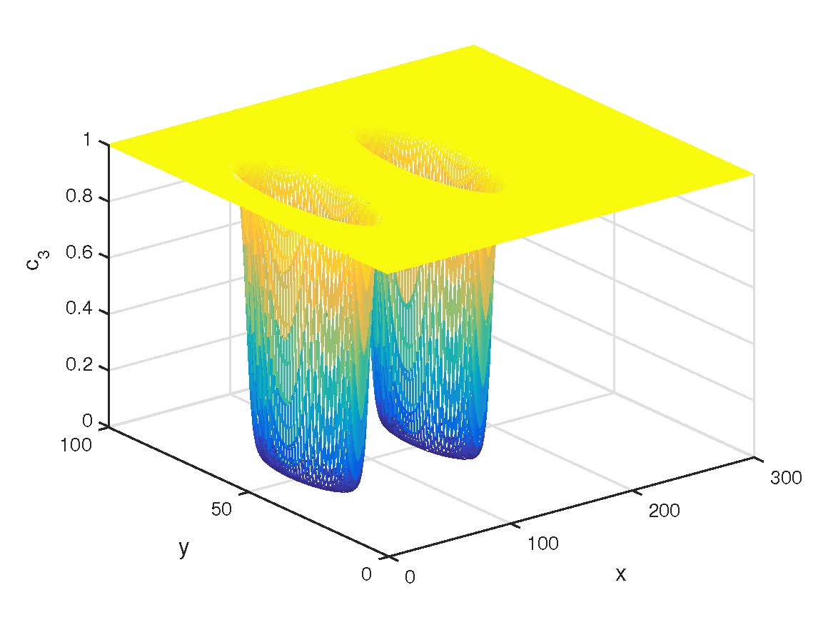
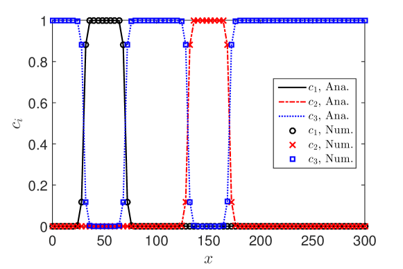
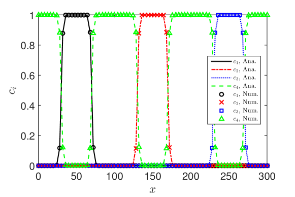
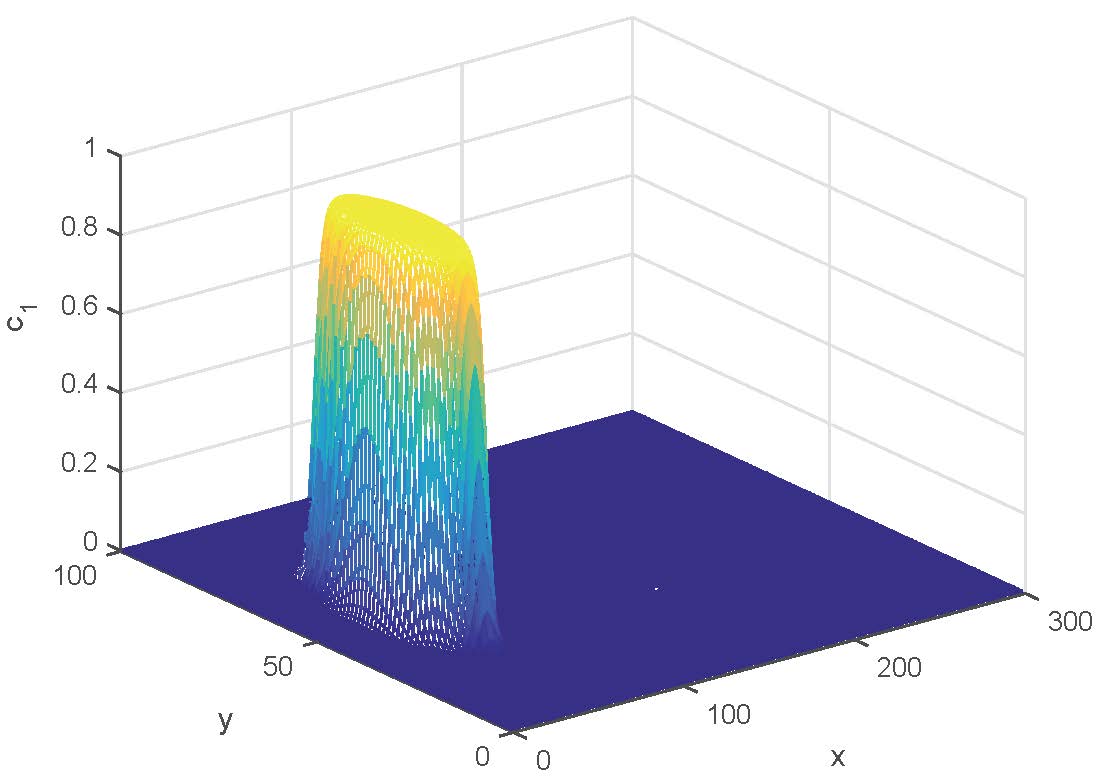
where σmin=minσijsubscript𝜎𝑚𝑖𝑛subscript𝜎𝑖𝑗\sigma_{min}=\min{\sigma_{ij}} is the minimum value among the 12N(N1)12𝑁𝑁1\frac{1}{2}N(N-1) surface tensions [4]. Here η𝜂\eta is set to η=2𝜂2\eta=\sqrt{2}, then β=0.06𝛽0.06\beta=\sqrt{0.06}. Fig. 1 shows the steady distributions of volume fractions obtained by the present LB model. It can be observed that the present LB model can accurately preserve the profiles of volume fractions with initial configurations for this 333-phase problem. In order to give quantitative comparisons, we also plot the volume fractions along the centerline (x=50𝑥50x=50, 0y3000𝑦3000\leq y\leq 300) in Fig. 2. From this figure, one can observe that the numerical results of the volume fractions agree well with the theoretical results.
Refer to caption
Refer to caption
Refer to caption
Figure 1: (Color online) The steady distributions of three volume fractions (c1subscript𝑐1c_{1}, c2subscript𝑐2c_{2}, c3subscript𝑐3c_{3}) obtained by the present LB model.
Refer to caption
Figure 2: (Color online) Volume fractions along the centerline (x=50𝑥50x=50, 0y3000𝑦3000\leq y\leq 300), where Ana. denotes analytical results and Num. denotes numerical results.

Besides, we also consider a 444-phase problem of static droplets. In this test, three droplets with radius R=20𝑅20R=20 are placed in the same domain of NX×NY=300×100𝑁𝑋𝑁𝑌300100NX\times NY=300\times 100. The initial volume fractions are expressed as

c1(x,y)=0.5+0.5tanhR(xxc1)2+(yyc1)22η,subscript𝑐1𝑥𝑦0.50.5𝑅superscript𝑥subscript𝑥subscript𝑐12superscript𝑦subscript𝑦subscript𝑐122𝜂\displaystyle c_{1}(x,y)=0.5+0.5\tanh\frac{R-\sqrt{(x-x_{c_{1}})^{2}+(y-y_{c_{1}})^{2}}}{\sqrt{2}\eta}, (53a)
c2(x,y)=0.5+0.5tanhR(xxc2)2+(yyc2)22η,subscript𝑐2𝑥𝑦0.50.5𝑅superscript𝑥subscript𝑥subscript𝑐22superscript𝑦subscript𝑦subscript𝑐222𝜂\displaystyle c_{2}(x,y)=0.5+0.5\tanh\frac{R-\sqrt{(x-x_{c_{2}})^{2}+(y-y_{c_{2}})^{2}}}{\sqrt{2}\eta}, (53b)
c3(x,y)=0.5+0.5tanhR(xxc3)2+(yyc3)22η,subscript𝑐3𝑥𝑦0.50.5𝑅superscript𝑥subscript𝑥subscript𝑐32superscript𝑦subscript𝑦subscript𝑐322𝜂\displaystyle c_{3}(x,y)=0.5+0.5\tanh\frac{R-\sqrt{(x-x_{c_{3}})^{2}+(y-y_{c_{3}})^{2}}}{\sqrt{2}\eta}, (53c)
c4(x,y)=1.0c1(x,y)c2(x,y)c3(x,y),subscript𝑐4𝑥𝑦1.0subscript𝑐1𝑥𝑦subscript𝑐2𝑥𝑦subscript𝑐3𝑥𝑦\displaystyle c_{4}(x,y)=1.0-c_{1}(x,y)-c_{2}(x,y)-c_{3}(x,y), (53d)

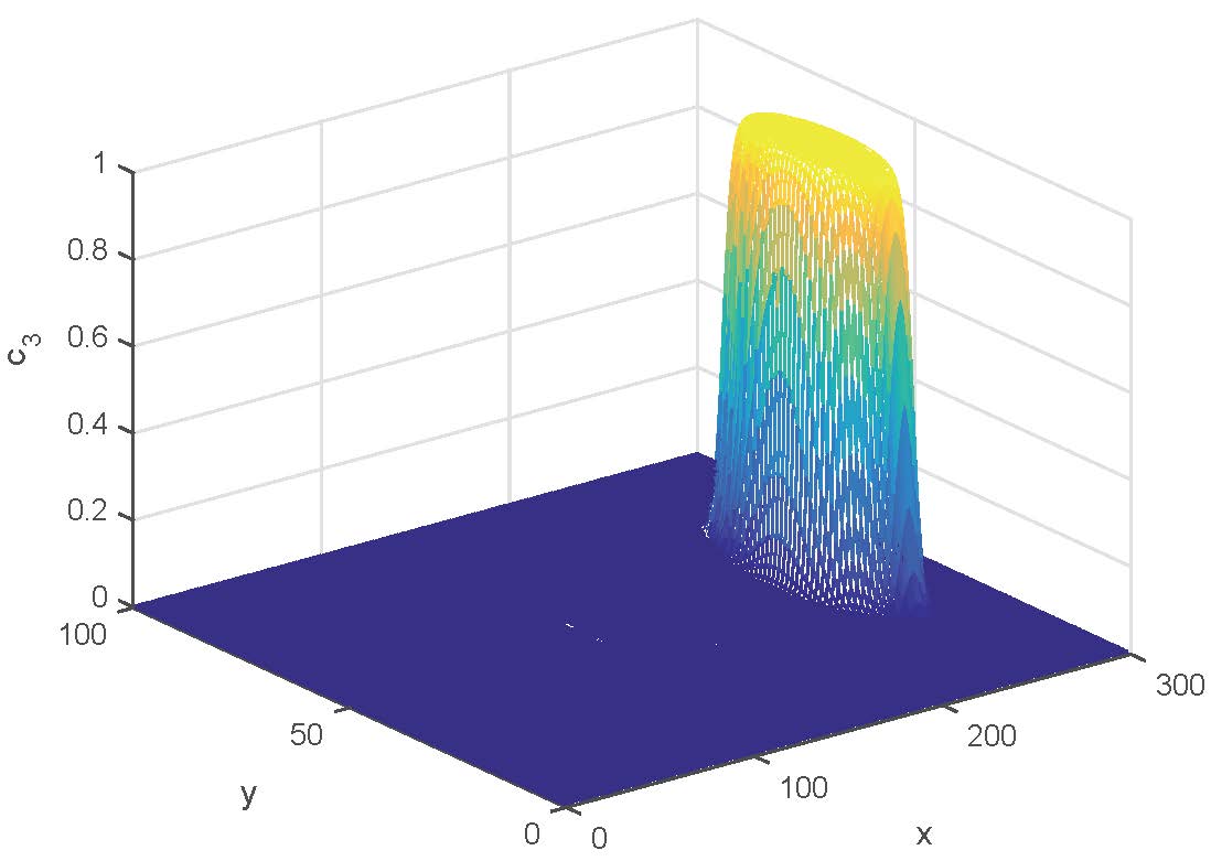
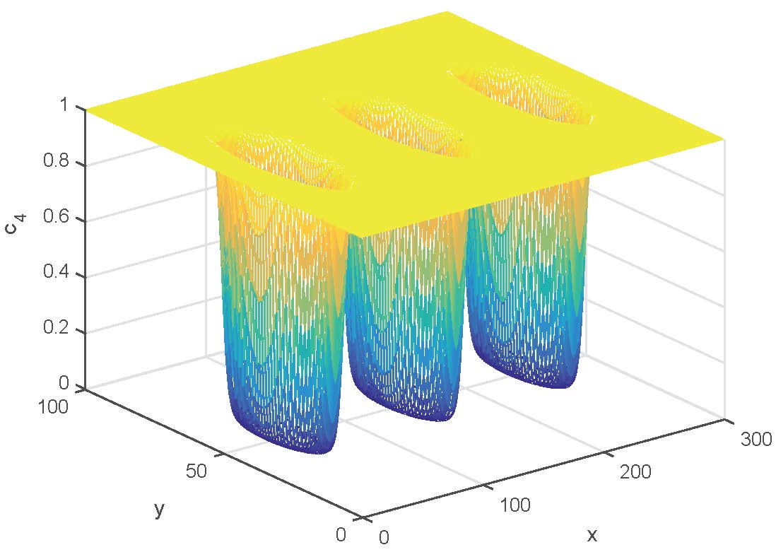
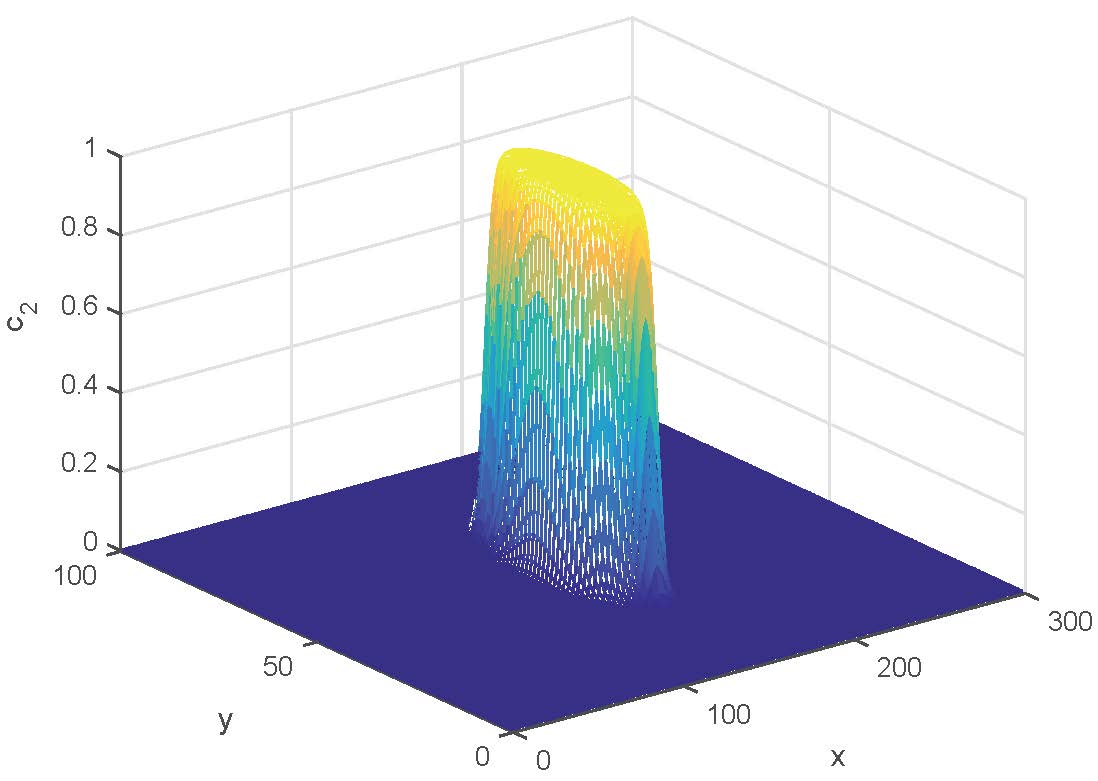
with (xc1,yc1)=(50,50)subscript𝑥subscript𝑐1subscript𝑦subscript𝑐15050(x_{c_{1}},y_{c_{1}})=(50,50), (xc2,yc2)=(150,50)subscript𝑥subscript𝑐2subscript𝑦subscript𝑐215050(x_{c_{2}},y_{c_{2}})=(150,50) and (xc3,yc3)=(250,50)subscript𝑥subscript𝑐3subscript𝑦subscript𝑐325050(x_{c_{3}},y_{c_{3}})=(250,50). Some other parameters are given as ρ1:ρ2:ρ3:ρ4=20:1:10:5:subscript𝜌1subscript𝜌2:subscript𝜌3:𝜌420:1:10:5\rho_{1}:\rho_{2}:\rho_{3}:\rho 4=20:1:10:5, τg=τ1=τ2=τ3=0.8subscript𝜏𝑔subscript𝜏1subscript𝜏2subscript𝜏30.8\tau_{g}=\tau_{1}=\tau_{2}=\tau_{3}=0.8, σ12=σ13=σ14=σ23=σ24=σ34=0.01subscript𝜎12subscript𝜎13subscript𝜎14subscript𝜎23subscript𝜎24𝜎340.01\sigma_{12}=\sigma_{13}=\sigma_{14}=\sigma_{23}=\sigma_{24}=\sigma{34}=0.01, m1=m2=m3=0.001subscript𝑚1subscript𝑚2subscript𝑚30.001m_{1}=m_{2}=m_{3}=0.001. The rest of the parameters are set as previous case. As shown in Fig. 3, the present LB model can also accurately preserve the profiles of volume fractions with initial configurations for 444-phase problems. To further give a detailed comparison, we also plot the volume fractions along the center line and compare the results between analytical results and numerical results. The results show that the developed LB model is accurate enough to simulate multiphase problems.

Refer to caption
Refer to caption
Refer to caption
Refer to caption
Figure 3: (Color online) The steady distributions of three volume fractions (c1subscript𝑐1c_{1}, c2subscript𝑐2c_{2}, c3subscript𝑐3c_{3}, c4subscript𝑐4c_{4}) obtained by the present LB model.
Refer to caption
Figure 4: (Color online) Volume fractions along the centerline (x=50𝑥50x=50, 0y3000𝑦3000\leq y\leq 300), where Ana. denotes analytical results and Num. denotes numerical results.

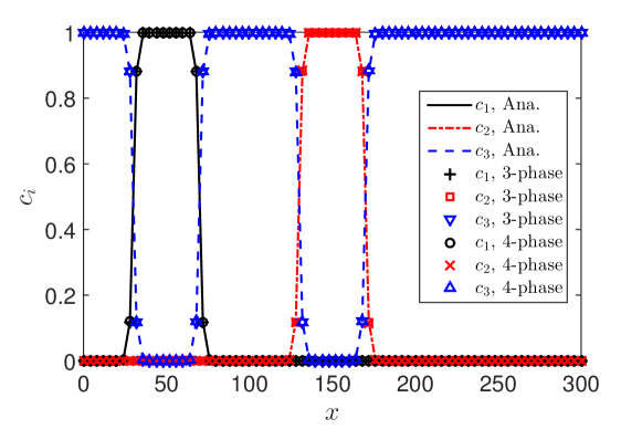
Next, we will show that our LB model for N𝑁N-phase flows can satisfy the reduction-consistent property. Here, the reduction-consistent property means that when one phase of the N𝑁N-phase system disappears, the designed model can still be used to simulate the remaining (N1𝑁1N-1)-phase system. Consider the case where the volume fraction of the third phase is 00 in the previous 444-phase example. The remaining parts can be viewed as a 333-phase system. For convenience, the 444th-phase in the former case is marked as the 333th-phase. Fig. 5 depicts the comparisons of volume fractions obtained from our 333-phase model, 444-phase model with one phase disappeared, and theoretical values along the centerline. It can be seen that the results from our 333-phase model and 444-phase model with one phase disappeared are almost identical, and they are also in good agreement with the theoretical values. Thus, we conclude that our LB model can satisfy the reduction-consistent property.
Refer to caption
Figure 5: (Color online) Comparisons of volume fractions obtained from our 333-phase model and 444-phase model with one phase disappeared as well as theoretical values along the centerline (x=50𝑥50x=50, 0y3000𝑦3000\leq y\leq 300).

4.2 Spreading of a liquid lens

Here we consider a droplet located at the interface between the other two immiscible fluids. Under the influence of surface tension, the droplet will form a lens when the system reaches equilibrium. According to Neumann’s law [48], the following relationships are satisfied between the contact angles and the surface tensions at the equilibrium state,

cos(θ1)=σ122+σ232σ1322σ12σ23,cos(θ2)=σ132+σ232σ1222σ13σ23,formulae-sequencesubscript𝜃1superscriptsubscript𝜎122superscriptsubscript𝜎232superscriptsubscript𝜎1322subscript𝜎12subscript𝜎23subscript𝜃2superscriptsubscript𝜎132superscriptsubscript𝜎232superscriptsubscript𝜎1222subscript𝜎13subscript𝜎23\cos(\theta_{1})=\frac{\sigma_{12}^{2}+\sigma_{23}^{2}-\sigma_{13}^{2}}{2\sigma_{12}\sigma_{23}},\quad\cos(\theta_{2})=\frac{\sigma_{13}^{2}+\sigma_{23}^{2}-\sigma_{12}^{2}}{2\sigma_{13}\sigma_{23}}, (54)

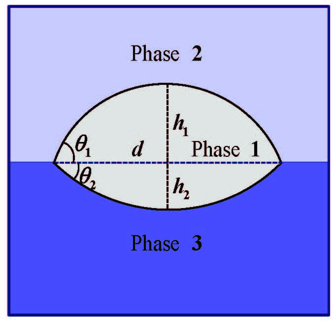
where θisubscript𝜃𝑖\theta_{i} (i=1,2𝑖12i=1,2) denote the contact angles as shown in Fig. 6. The relationship between the lens area A𝐴A, its length d𝑑d (the distance between two triple junctions) and the contact angles is

A=(d2)2i=121sin(θi)(θisinθicosθi),𝐴superscript𝑑22superscriptsubscript𝑖121subscript𝜃𝑖subscript𝜃𝑖subscript𝜃𝑖subscript𝜃𝑖A=\left(\frac{d}{2}\right)^{2}\sum_{i=1}^{2}\frac{1}{\sin(\theta_{i})}\left(\frac{\theta_{i}}{\sin\theta_{i}}-\cos\theta_{i}\right), (55)

After some simple geometric transformations, we can derive the following expression

hi=(d2)1cosθisinθi,i=1,2.formulae-sequencesubscript𝑖𝑑21subscript𝜃𝑖subscript𝜃𝑖𝑖12h_{i}=\left(\frac{d}{2}\right)\frac{1-\cos\theta_{i}}{\sin\theta_{i}},\quad i=1,2. (56)
Refer to caption
Figure 6: (Color online) Schematic of the lens shape at the equilibrium state.

Initially, a circular droplet with the radius R=30𝑅30R=30 is placed in the middle of the computational domain with NX×NY=150×150𝑁𝑋𝑁𝑌150150NX\times NY=150\times 150. The initial volume fractions are given by

c1(x,y)=0.5+0.5tanhR(xxc)2+(yyc)22η,subscript𝑐1𝑥𝑦0.50.5𝑅superscript𝑥subscript𝑥𝑐2superscript𝑦subscript𝑦𝑐22𝜂\displaystyle c_{1}(x,y)=0.5+0.5\tanh\frac{R-\sqrt{(x-x_{c})^{2}+(y-y_{c})^{2}}}{\sqrt{2}\eta}, (57a)
c2(x,y)=max[0.5+0.5tanhyyc2ηc1(x,y),0],subscript𝑐2𝑥𝑦0.50.5𝑦subscript𝑦𝑐2𝜂subscript𝑐1𝑥𝑦0\displaystyle c_{2}(x,y)=\max\left[0.5+0.5\tanh\frac{y-y_{c}}{\sqrt{2}\eta}-c_{1}(x,y),0\right], (57b)
c3(x,y)=1.0c1(x,y)c2(x,y),subscript𝑐3𝑥𝑦1.0subscript𝑐1𝑥𝑦subscript𝑐2𝑥𝑦\displaystyle c_{3}(x,y)=1.0-c_{1}(x,y)-c_{2}(x,y), (57c)

where (xc,yc)subscript𝑥𝑐subscript𝑦𝑐(x_{c},y_{c}) is the coordinate of circular droplet.

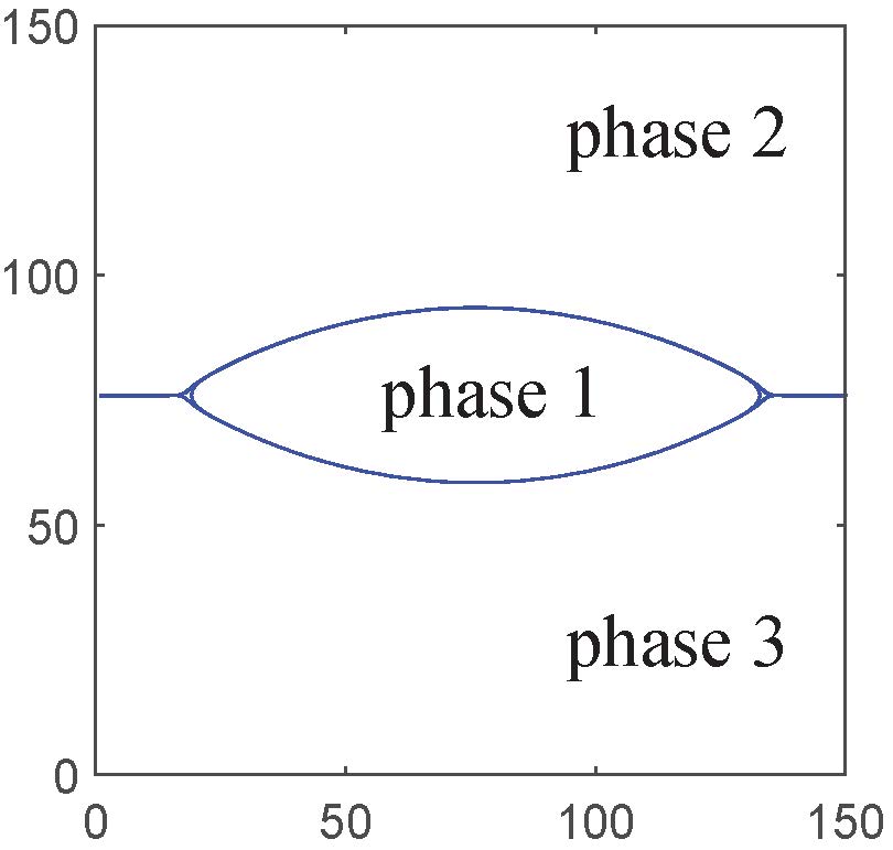
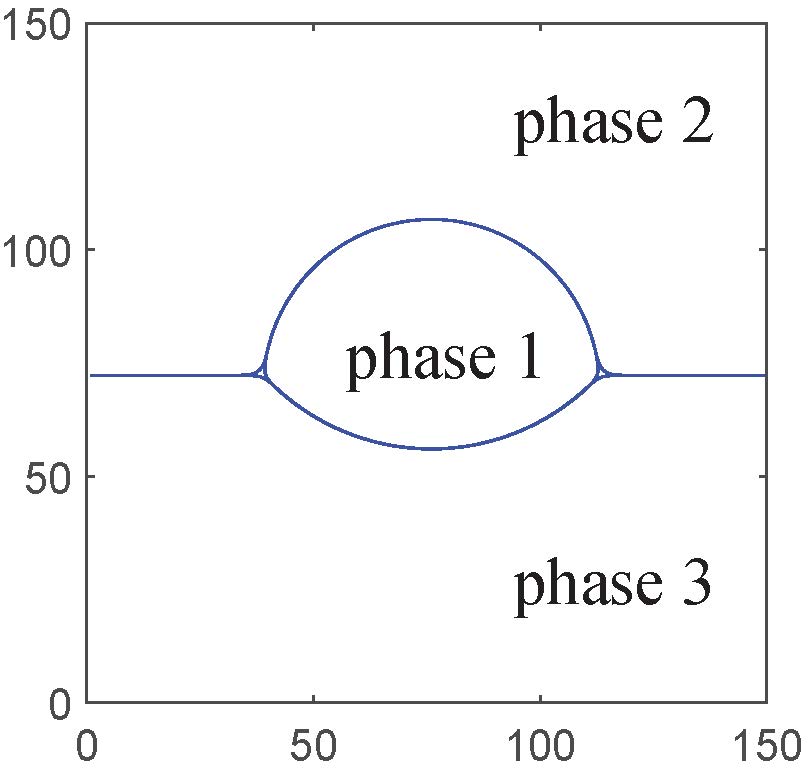
In this test, the periodic boundary conditions are employed in the x𝑥x-direction, and the halfway bounce-back boundary conditions are enforced on the top and bottom walls. The density ratio of the three fluids is set to ρ1:ρ2:ρ3=10:1:5:subscript𝜌1subscript𝜌2:subscript𝜌310:1:5\rho_{1}:\rho_{2}:\rho_{3}=10:1:5. Some other physical parameters are given as τg=τ1=τ2=0.8subscript𝜏𝑔subscript𝜏1subscript𝜏20.8\tau_{g}=\tau_{1}=\tau_{2}=0.8, σ12:σ13:σ23=1:43:1:subscript𝜎12subscript𝜎13:subscript𝜎231:43:1\sigma_{12}:\sigma_{13}:\sigma_{23}=1:\frac{4}{3}:1, 1:1:1:11:11:1:1, and 0.6:0.6:1:0.60.6:10.6:0.6:1, m1=m2=0.1subscript𝑚1subscript𝑚20.1m_{1}=m_{2}=0.1, η=2𝜂2\eta=\sqrt{2}, β=0.06𝛽0.06\beta=\sqrt{0.06}. It is shown in Fig. 7 that the droplets will undergo some deformations due to the effect of surface tension, and eventually form distinct equilibrium configurations. The shapes of the liquid interface in this work are in good agreement with the previous results [49, 23]. In order to give quantitative results, we also measured the contact angles θ1subscript𝜃1\theta_{1} and θ2subscript𝜃2\theta_{2} and compared them with the analytical solutions (see Table 1), where the numerical solutions θ1subscript𝜃1\theta_{1} and θ2subscript𝜃2\theta_{2} are calculated by

θ1=2arctan(2h1d),θ2=2arctan(2h2d).formulae-sequencesubscript𝜃122subscript1𝑑subscript𝜃222subscript2𝑑\theta_{1}=2\arctan\left(\frac{2h_{1}}{d}\right),\quad\theta_{2}=2\arctan\left(\frac{2h_{2}}{d}\right). (58)

From Table 1, one can observe that the numerical contact angles θ1subscript𝜃1\theta_{1} and θ2subscript𝜃2\theta_{2} are in good agreement with analytical solutions, where the maximum relative errors are no more than 1.5%percent1.51.5\%. In addition, we also give a comparison between the numerical solutions and the analytical solutions of the length d𝑑d and the height (h1,h2)subscript1subscript2(h_{1},h_{2}), see Table 2. It is shown that the maximum relative errors of d𝑑d, h1subscript1h_{1} and h2subscript2h_{2} shall not exceed 1.8%percent1.81.8\%, which means that the present LB model can accurately capture the interface of the incompressible three-phase flow without considering gravity.
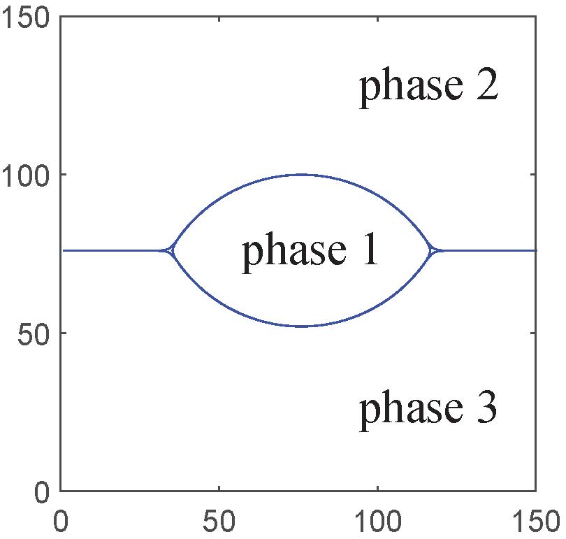
Refer to caption
Refer to caption
Refer to caption
Figure 7: (Color online) Schematic of the lens shape at the equilibrium state.
Table 1: The equilibrium contact angles θ1subscript𝜃1\theta_{1} and θ2subscript𝜃2\theta_{2} with different surface tension ratios.
Surface tension Present LB model Analytical solutions Relative errors
(σ12:σ13:σ23):subscript𝜎12subscript𝜎13:subscript𝜎23(\sigma_{12}:\sigma_{13}:\sigma_{23}) θ1subscript𝜃1\theta_{1} θ2subscript𝜃2\theta_{2} θ1subscript𝜃1\theta_{1} θ2subscript𝜃2\theta_{2} θ1subscript𝜃1\theta_{1} θ2subscript𝜃2\theta_{2}
1:43:1:143:11:\frac{4}{3}:1 84.6superscript84.684.6^{\circ} 50.0superscript50.050.0^{\circ} 83.5superscript83.583.5^{\circ} 52.5superscript52.552.5^{\circ} 1.2%percent1.21.2\% 0.2%percent0.20.2\%
1:1:1:11:11:1:1 60.7superscript60.760.7^{\circ} 60.7superscript60.760.7^{\circ} 60.0superscript60.060.0^{\circ} 60.0superscript60.060.0^{\circ} 1.2%percent1.21.2\% 1.2%percent1.21.2\%
0.6:0.6:1:0.60.6:10.6:0.6:1 34.1superscript34.134.1^{\circ} 34.1superscript34.134.1^{\circ} 34.0superscript34.034.0^{\circ} 34.0superscript34.034.0^{\circ} 1.5%percent1.51.5\% 1.5%percent1.51.5\%
Table 2: The equilibrium length d𝑑d and height (h1,h2)subscript1subscript2(h_{1},h_{2}) with different surface tension ratios.
Surface tension Present LB model Analytical solutions Relative errors
(σ12:σ13:σ23):subscript𝜎12subscript𝜎13:subscript𝜎23(\sigma_{12}:\sigma_{13}:\sigma_{23}) d𝑑d h1subscript1h_{1} h2subscript2h_{2} d𝑑d h1subscript1h_{1} h2subscript2h_{2} d𝑑d h1subscript1h_{1} h2subscript2h_{2}
1:43:1:143:11:\frac{4}{3}:1 73.073.073.0 33.233.233.2 16.316.316.3 73.873.873.8 33.033.033.0 16.516.516.5 1.1%percent1.11.1\% 0.6%percent0.60.6\% 1.2%percent1.21.2\%
1:1:1:11:11:1:1 82.082.082.0 23.623.623.6 23.623.623.6 80.780.780.7 23.323.323.3 23.323.323.3 1.7%percent1.71.7\% 1.3%percent1.31.3\% 1.3%percent1.31.3\%
0.6:0.6:1:0.60.6:10.6:0.6:1 114.0114.0114.0 17.517.517.5 17.517.517.5 113.9113.9113.9 17.217.217.2 17.217.217.2 0.1%percent0.10.1\% 1.8%percent1.81.8\% 1.8%percent1.81.8\%

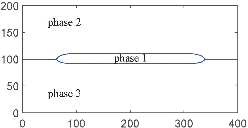
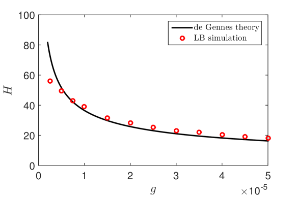
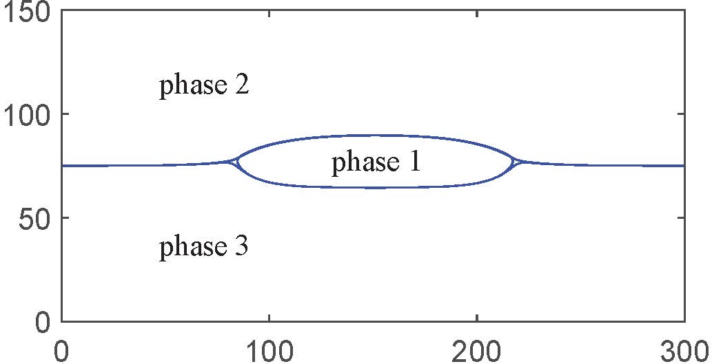
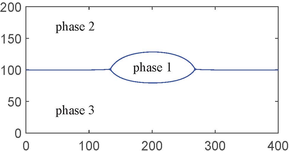
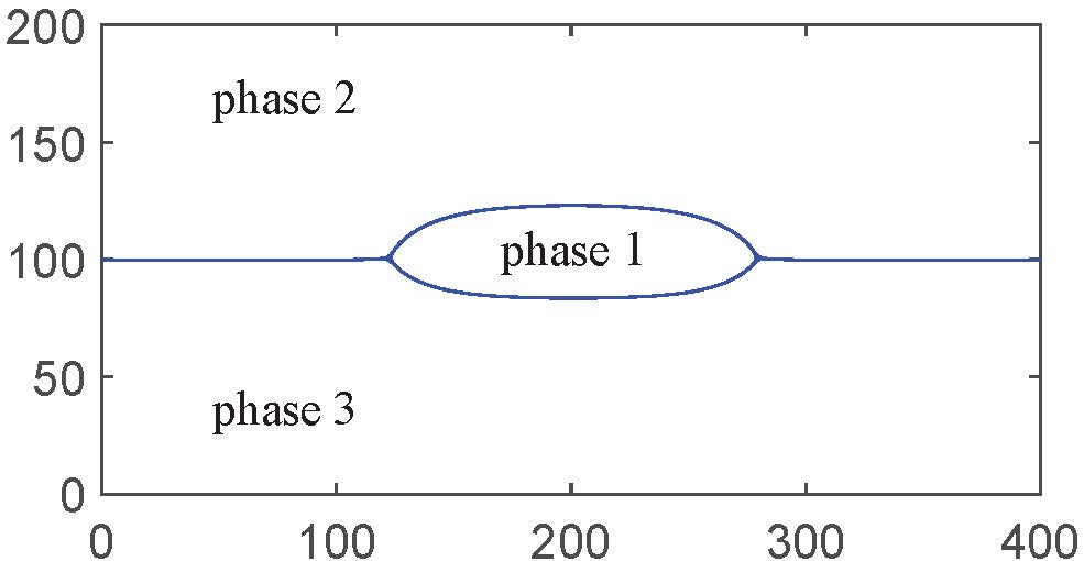
Furthermore, now we consider the effect of gravity on the equilibrium configurations. To generate the gravitational effects, a body force, 𝐆=(0,ρg)𝐆0𝜌𝑔\mathbf{G}=(0,\rho g), is added to the momentum equation, where g𝑔g is the gravitational acceleration. In this test, we vary the value of the gravitational acceleration while fixing all the other physical parameters. Due to the large deformation of the interface, the computational domain is set to NX×NY=400×200𝑁𝑋𝑁𝑌400200NX\times NY=400\times 200. The physical parameters are given as ρ1:ρ2:ρ3=3:1:6:subscript𝜌1subscript𝜌2:subscript𝜌33:1:6\rho_{1}:\rho_{2}:\rho_{3}=3:1:6, τg=τ1=τ2=0.8subscript𝜏𝑔subscript𝜏1subscript𝜏20.8\tau_{g}=\tau_{1}=\tau_{2}=0.8, σ12:σ13:σ23=1:1:1:subscript𝜎12subscript𝜎13:subscript𝜎231:1:1\sigma_{12}:\sigma_{13}:\sigma_{23}=1:1:1, m1=m2=0.1subscript𝑚1subscript𝑚20.1m_{1}=m_{2}=0.1. As shown in Fig. 8, when the gravity is relatively small and surface tension is dominant, the droplet forms a lens on the water surface. As the gravity increases, the droplet becomes flatter [see Fig. 8]. When the gravity is large enough and dominates over the surface tension, it will forms a puddle [see Fig. 8]. The current results are qualitatively consistent with the de Gennes theory [52]. To give a quantitative comparison, we measured asymptotic thickness H𝐻H as a function of gravity and compared it with the de Gennes theory, where the asymptotic puddle thickness can be given as [52, 53]

H=2(σ12+σ13σ23)ρ1ρ3(ρ3ρ1)g.𝐻2subscript𝜎12subscript𝜎13subscript𝜎23subscript𝜌1subscript𝜌3subscript𝜌3subscript𝜌1𝑔H=\sqrt{\frac{2(\sigma_{12}+\sigma_{13}-\sigma_{23})}{\frac{\rho_{1}}{\rho_{3}}(\rho_{3}-\rho_{1})g}}. (59)

Fig. 9 depicts the asymptotic thickness as a function of gravity between the present results and the de Gennes theory. One can observe that the present results agree well with the de Gennes theory when the gravity is large (g0.5𝑔0.5g\geq 0.5 for this case). However, when the gravity is small, a large discrepancy between the numerical results and theoretical results, because the expression (59) is not valid for the case that g𝑔g is too small [4].

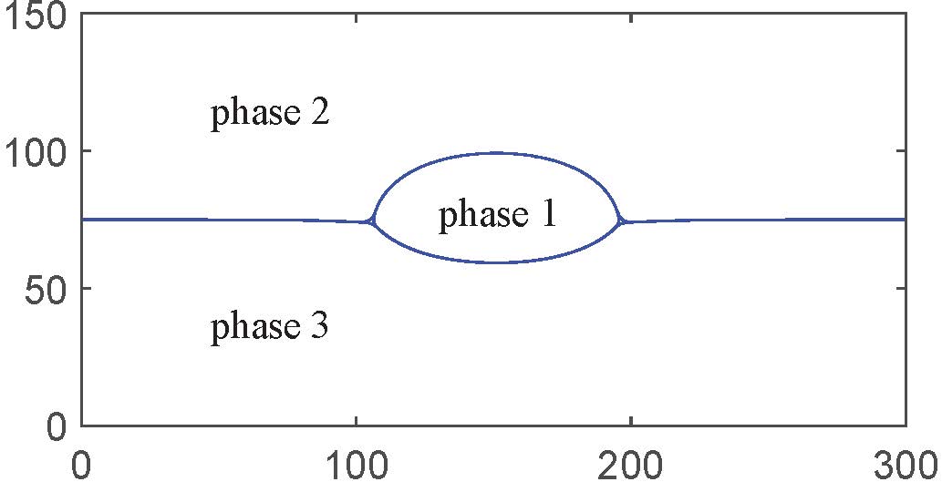
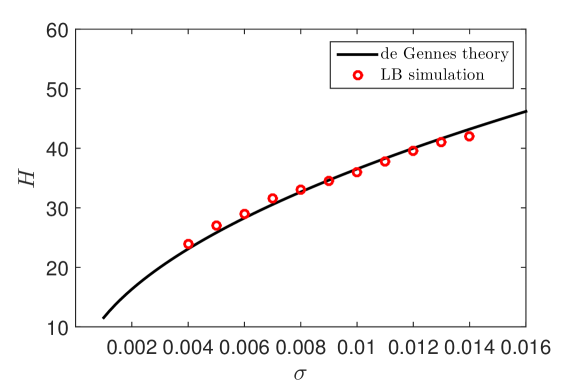
In addition, we also consider the effect of surface tension on the equilibrium configurations. In this test, we fix the gravitational acceleration g𝑔g and the surface tensions σ12subscript𝜎12\sigma_{12}, σ23subscript𝜎23\sigma_{23} to g=1×10⁵𝑔1superscript105g=1\times 10^{-5}, σ12=σ23=0.01subscript𝜎12subscript𝜎230.01\sigma_{12}=\sigma_{23}=0.01 and vary the surface tension σ13subscript𝜎13\sigma_{13}. The computational domain is set to NX×NY=300×150𝑁𝑋𝑁𝑌300150NX\times NY=300\times 150. The other parameters are the same as the previous test. As shown in Fig. 10, the droplet thickness strongly depend on the surface tension. As the surface tension increases, the droplet thickness gradually increases. To quantitatively describe the relationship between asymptotic thickness and surface tension, we give a comparison of the results between the current simulation and the de Gennes theory [52] (see Fig. 11). From Fig. 11, one can conclude that H𝐻H and σ13subscript𝜎13\sigma_{13} increase simultaneously, and the simulation results are in good agreement with the de Gennes theory.

Therefore, all the results of this section, especially qualitative and quantitative comparisons with de Gennes theory, show that the current LB model is accurate and efficient for simulating the motion of incompressible multiphase systems.
Refer to caption
Refer to caption
Refer to caption
Figure 8: (Color online) The equilibrium configurations of the droplet with different gravity forces: (a) g=5×10⁶𝑔5superscript106g=5\times 10^{-6}, (b) 1×1051superscript1051\times 10^{-5}, (c) g=5×10⁵𝑔5superscript105g=5\times 10^{-5}.
Refer to caption
Figure 9: (Color online) Comparison of the asymptotic puddle thickness H𝐻H as a function of gravity g𝑔g between the present results and the de Gennes theory.
Refer to caption
Refer to caption
Figure 10: (Color online) The equilibrium configurations of the droplet with different surface tensions: (a) σ13=0.004subscript𝜎130.004\sigma_{13}=0.004, (b) σ13=0.014subscript𝜎130.014\sigma_{13}=0.014. Here the gravitational acceleration is fixed to g=1×10⁵𝑔1superscript105g=1\times 10^{-5}

.

Refer to caption
Figure 11: (Color online) Comparison of the asymptotic puddle thickness H𝐻H as a function of surface tension σ13subscript𝜎13\sigma_{13} between the present results and the de Gennes theory.

5 Numerical applications

To further demonstrate the capabilities and performance of the LB model we proposed for N𝑁N-phase flows (N2𝑁2N\geq 2), two numerical applications involving four to five fluid phases are carried out. These applications include the dynamics of droplet collision for four fluid phases and dynamics of droplets and interfaces for five fluid phases. The simulation results show that the present LB model can be used to study the interactions among multiple types of fluid interfaces.

5.1 Dynamics of droplet collision for four fluid phases

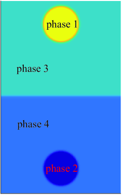
In this subsection, we study a dynamic problem involving four fluid phases as another test for validating the developed LB method. This phenomenon is very common in engineering and industrial problems, as well as in nature, such as in spraying processes, in micro-reactors, and in kitchen [55, 56, 4]. The problem configuration is shown in Fig. 12, where the upper part of the domain is filled with phase 333, and the lower part is filled with phase 444. One droplet, referred to as phase 111, is located inside phase 333. Simultaneously, a bubble of the same size, denoted as phase 222, is located in phase 444. Then, the droplet and the bubble start to move from rest under gravity (buoyancy). In this simulation, the computational domain is chosen as NY×NX=320×200𝑁𝑌𝑁𝑋320200NY\times NX=320\times 200. Periodic boundary conditions are applied in the horizonal direction, and the halfway bounce-back boundary conditions are enforced on the top and bottom walls. The initial volume fractions are given by

c1(x,y)=0.5+0.5tanhR(xxc1)2+(yyc1)22η,subscript𝑐1𝑥𝑦0.50.5𝑅superscript𝑥subscript𝑥subscript𝑐12superscript𝑦subscript𝑦subscript𝑐122𝜂\displaystyle c_{1}(x,y)=0.5+0.5\tanh\frac{R-\sqrt{(x-x_{c_{1}})^{2}+(y-y_{c_{1}})^{2}}}{\sqrt{2}\eta}, (60a)
c2(x,y)=0.5+0.5tanhR(xxc2)2+(yyc2)22η,subscript𝑐2𝑥𝑦0.50.5𝑅superscript𝑥subscript𝑥subscript𝑐22superscript𝑦subscript𝑦subscript𝑐222𝜂\displaystyle c_{2}(x,y)=0.5+0.5\tanh\frac{R-\sqrt{(x-x_{c_{2}})^{2}+(y-y_{c_{2}})^{2}}}{\sqrt{2}\eta}, (60b)
c3(x,y)=(0.5+0.5tanhyy02η)×[1.0c1(x,y)]subscript𝑐3𝑥𝑦0.50.5𝑦subscript𝑦02𝜂delimited-[]1.0subscript𝑐1𝑥𝑦\displaystyle c_{3}(x,y)=\left(0.5+0.5\tanh\frac{y-y_{0}}{\sqrt{2}\eta}\right)\times[1.0-c_{1}(x,y)] (60c)
c4(x,y)=1.0c1(x,y)c2(x,y)c3(x,y),subscript𝑐4𝑥𝑦1.0subscript𝑐1𝑥𝑦subscript𝑐2𝑥𝑦subscript𝑐3𝑥𝑦\displaystyle c_{4}(x,y)=1.0-c_{1}(x,y)-c_{2}(x,y)-c_{3}(x,y), (60d)

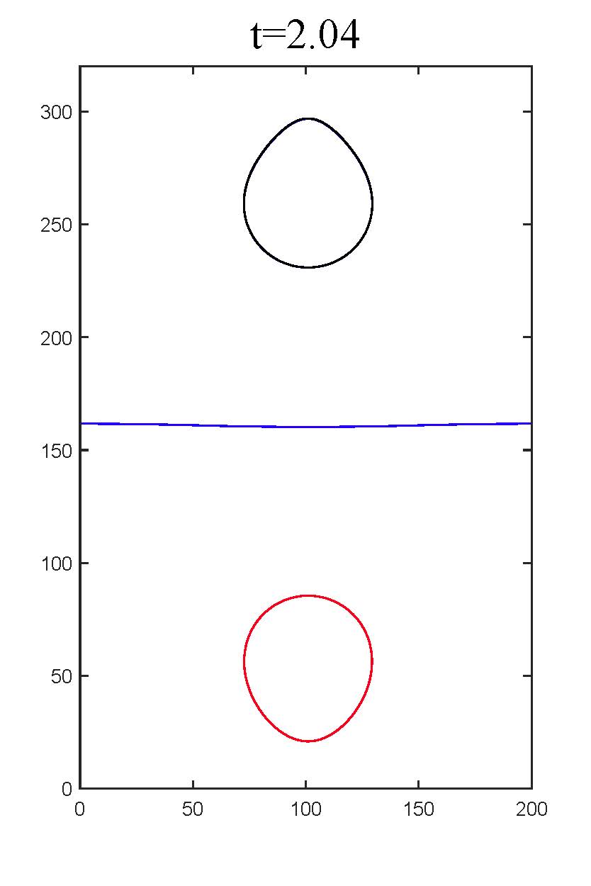
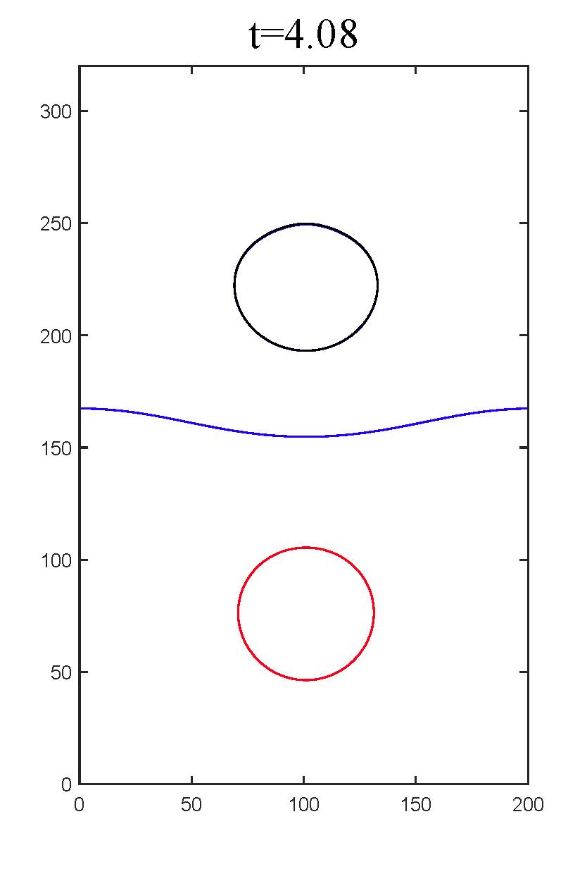
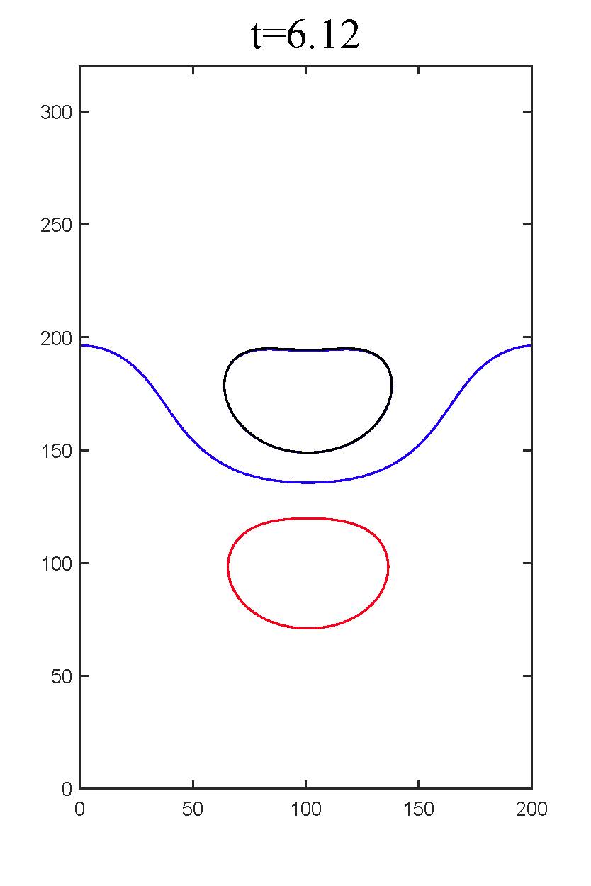
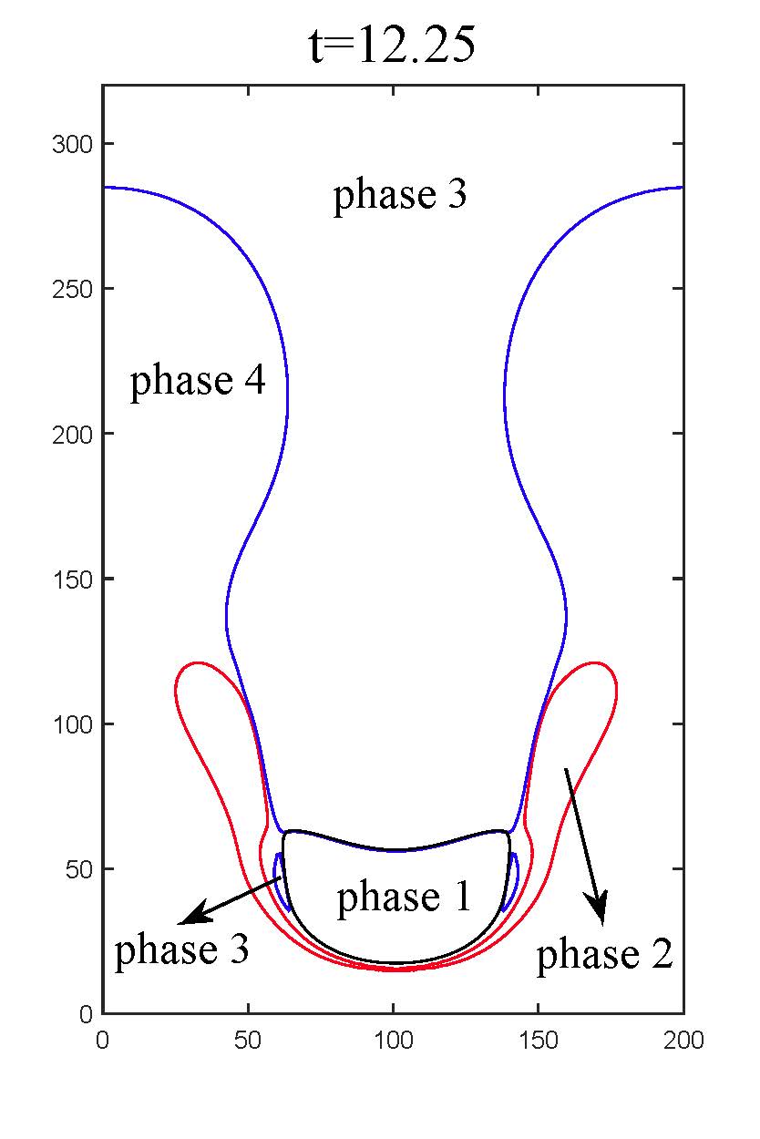
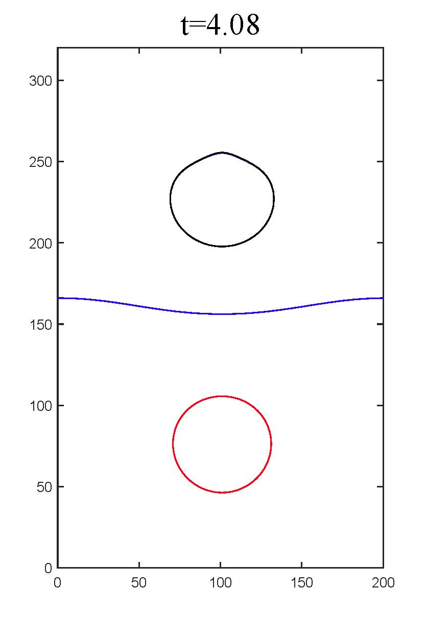
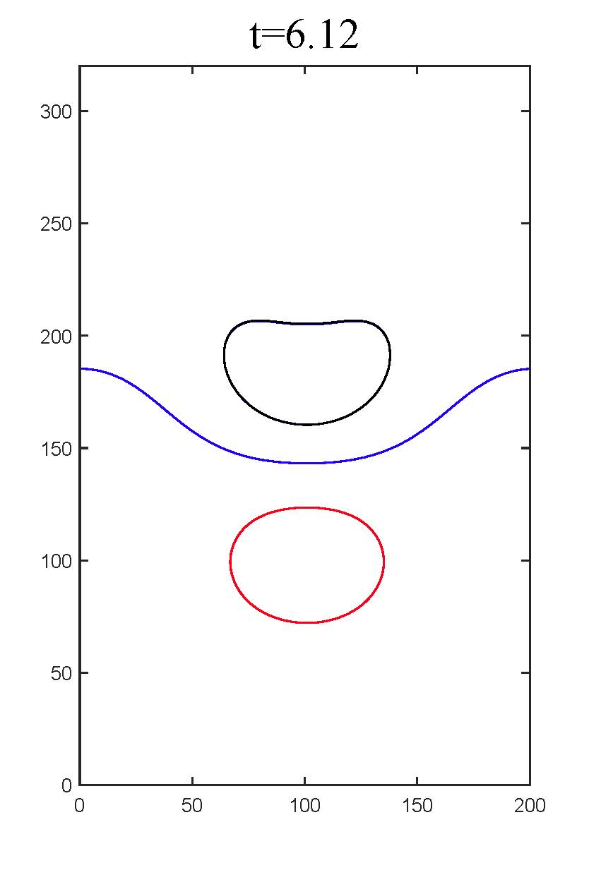
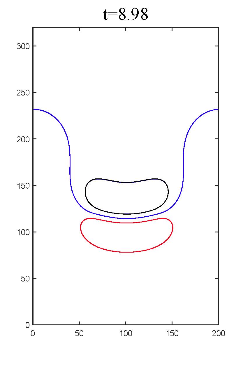
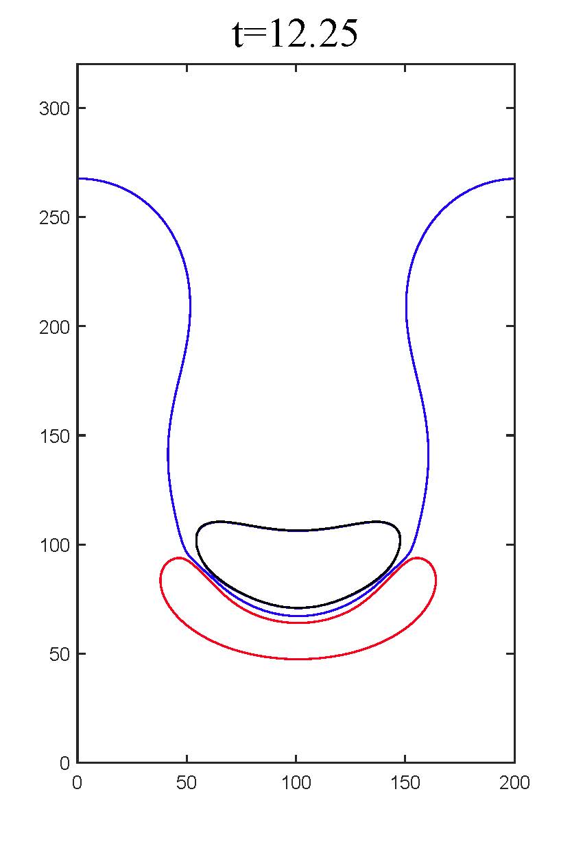
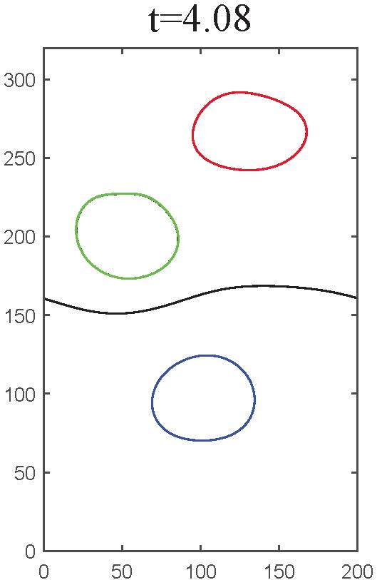
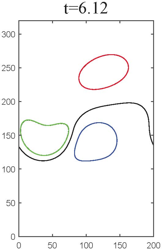
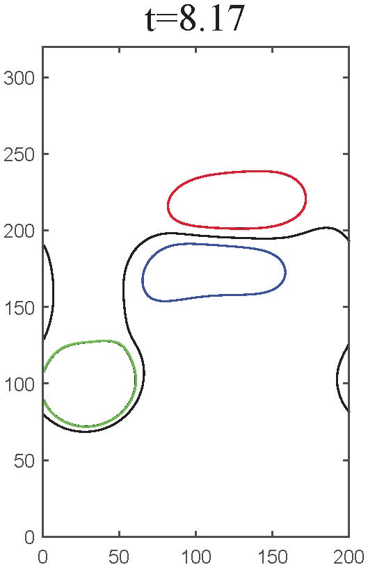
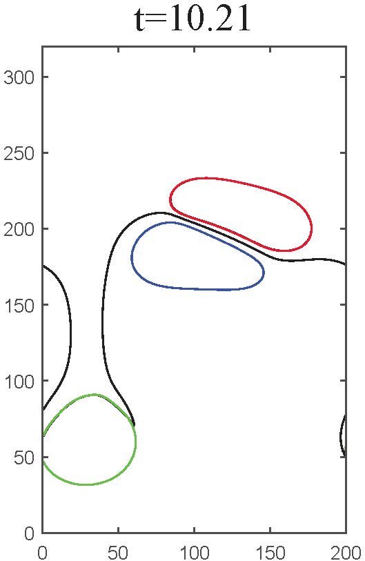
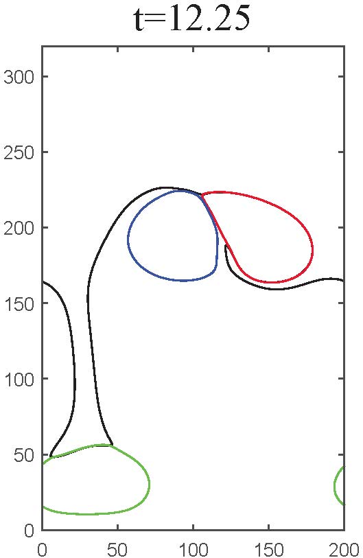
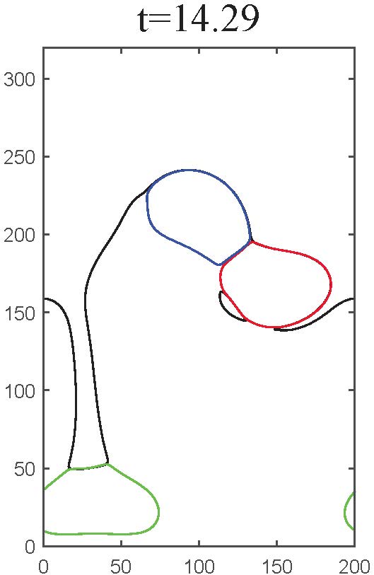
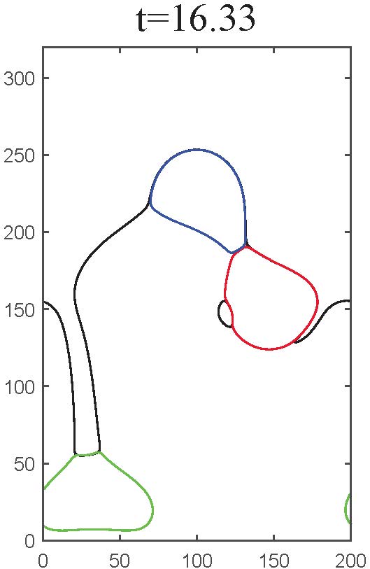
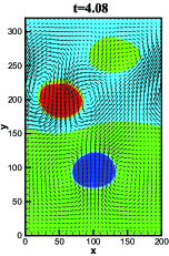
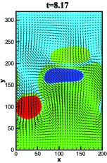
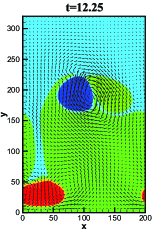
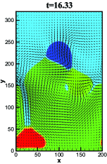
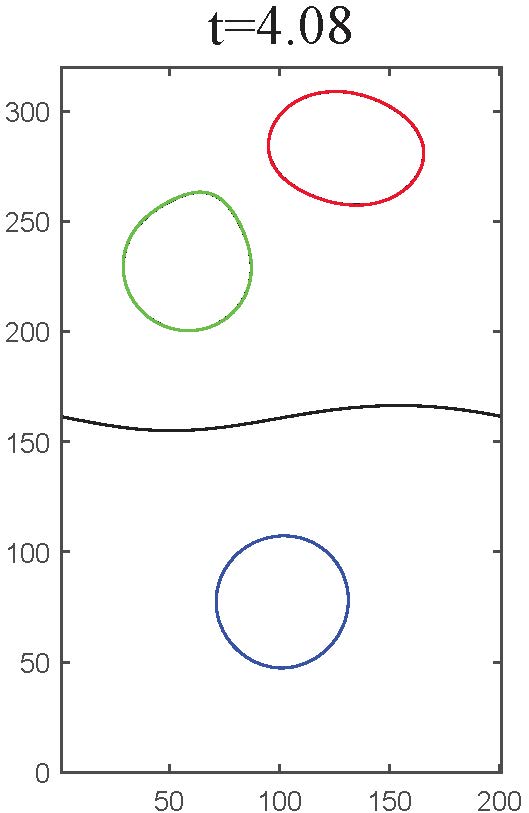
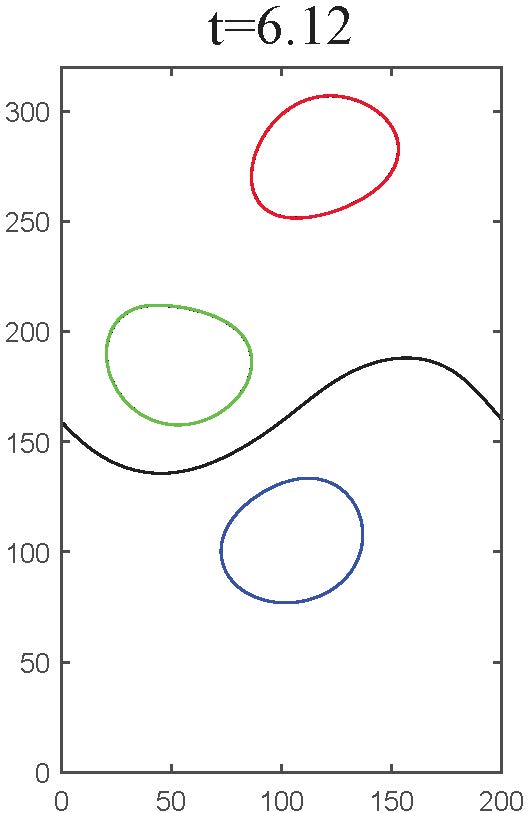
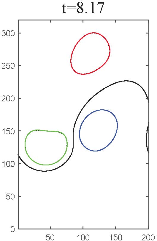
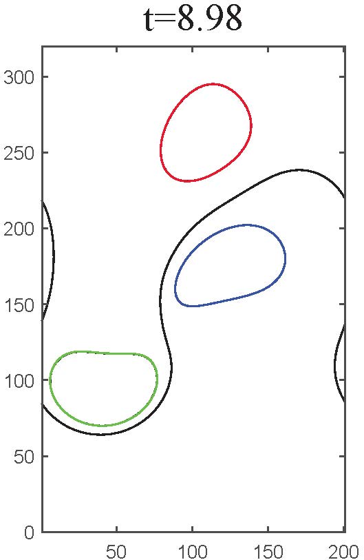
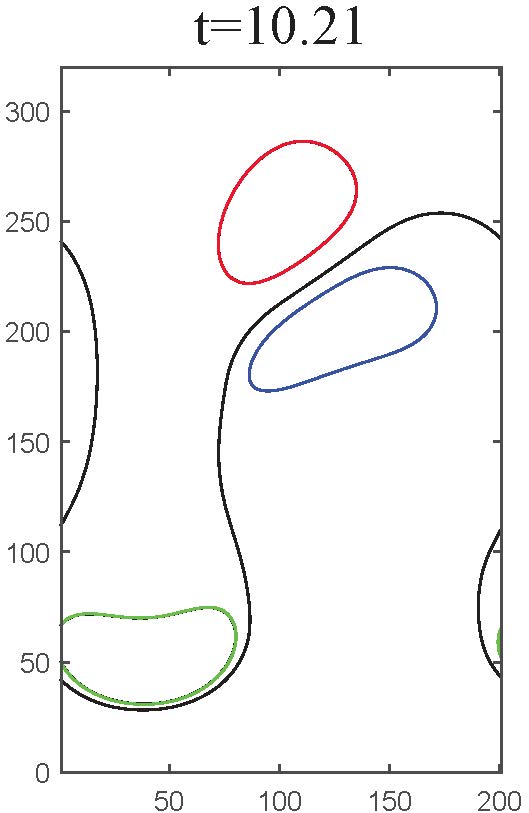
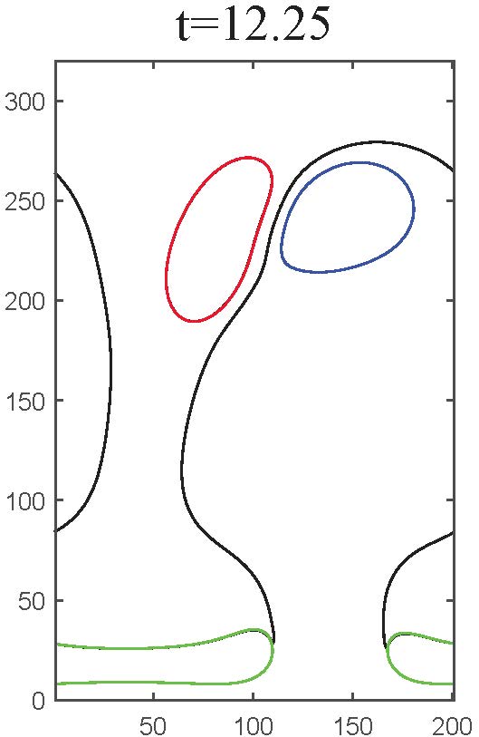
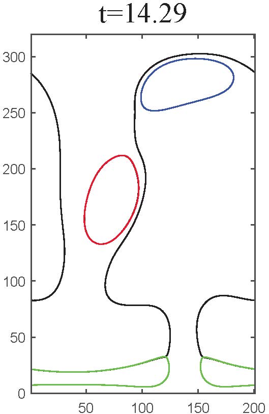
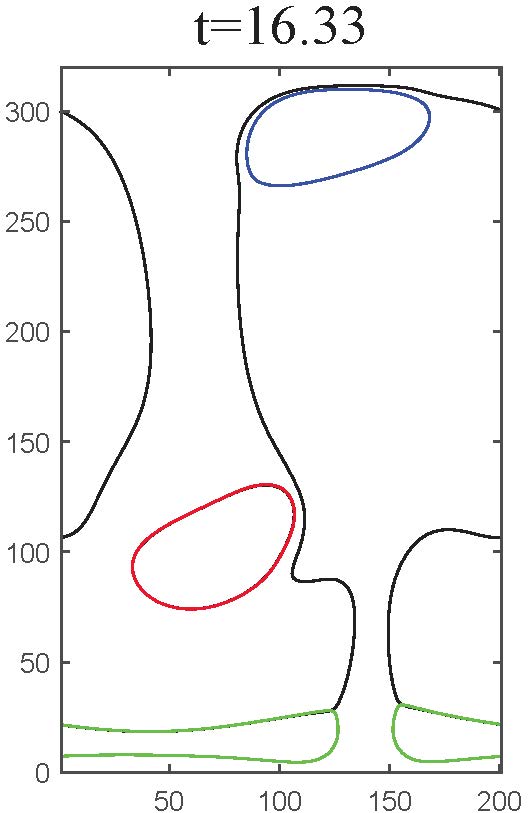
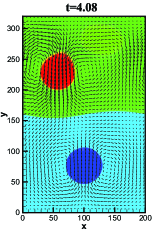
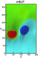
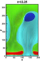
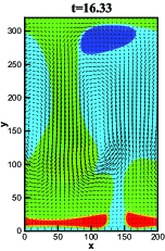
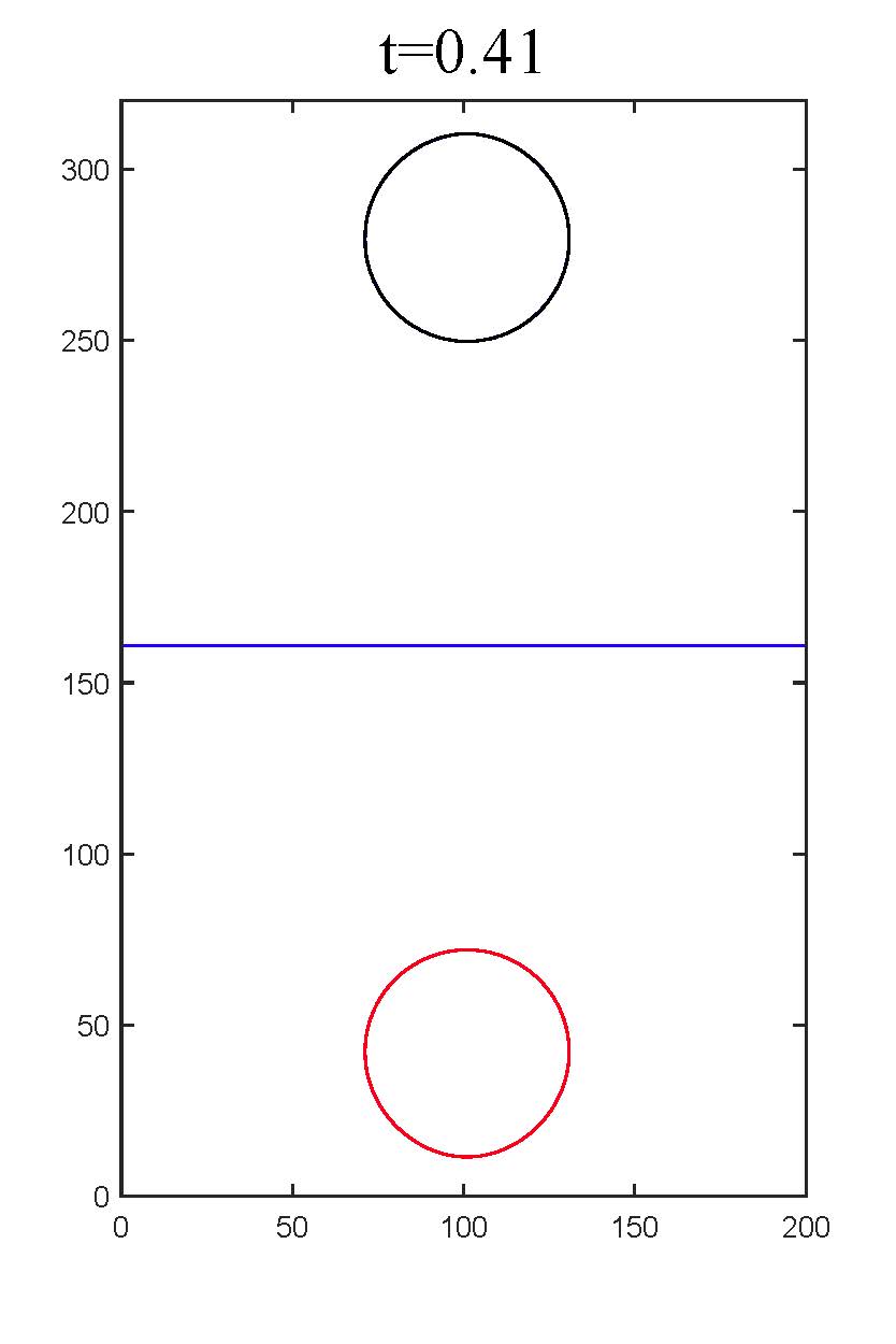
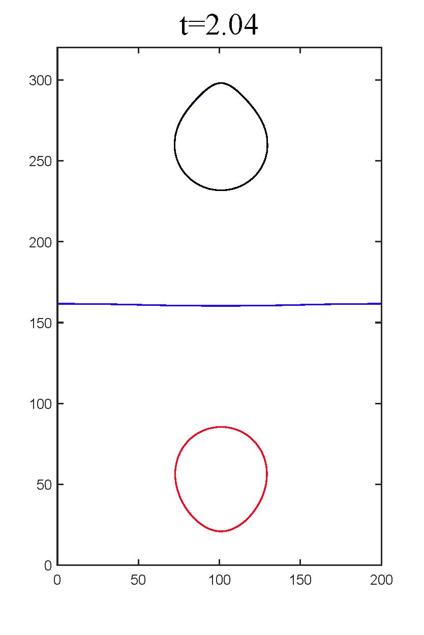
where (xc1,yc1)subscript𝑥subscript𝑐1subscript𝑦subscript𝑐1(x_{c_{1}},y_{c_{1}}) and (xc2,yc2)subscript𝑥subscript𝑐2subscript𝑦subscript𝑐2(x_{c_{2}},y_{c_{2}}) are the center of two droplets, and y0=12NYsubscript𝑦012𝑁𝑌y_{0}=\frac{1}{2}NY is the initial surface position between phase 333 and phase 444. Both of phase 111 and phase 222 have a diameter of D=60𝐷60D=60. Different values of surface tension σ13subscript𝜎13\sigma_{13} are investigated. The other parameters are fixed as ρ1:ρ2:ρ3:ρ4=6:1:3:2:subscript𝜌1subscript𝜌2:subscript𝜌3:subscript𝜌46:1:3:2\rho_{1}:\rho_{2}:\rho_{3}:\rho_{4}=6:1:3:2, σ12=σ14=σ23=σ24=σ34=0.01subscript𝜎12subscript𝜎14subscript𝜎23subscript𝜎24subscript𝜎340.01\sigma_{12}=\sigma_{14}=\sigma_{23}=\sigma_{24}=\sigma_{34}=0.01, τg=τ1=τ2=τ3=0.8subscript𝜏𝑔subscript𝜏1subscript𝜏2subscript𝜏30.8\tau_{g}=\tau_{1}=\tau_{2}=\tau_{3}=0.8, m1=m2=m3=0.1subscript𝑚1subscript𝑚2subscript𝑚30.1m_{1}=m_{2}=m_{3}=0.1, η=2𝜂2\eta=\sqrt{2}, β=0.06𝛽0.06\beta=\sqrt{0.06}, g=105𝑔superscript105g=10^{-5}, (xc1,yc1)=(160,280)subscript𝑥𝑐1subscript𝑦𝑐1160280(x_{c1},y_{c1})=(160,280), (xc2,yc2)=(160,40)subscript𝑥𝑐2subscript𝑦𝑐216040(x_{c2},y_{c2})=(160,40). Fig. 13 shows the time sequence of evolution of the fluid interfaces with σ13=0.01subscript𝜎130.01\sigma_{13}=0.01, where the solid line represents the contour levels of the volume fraction ci=0.5subscript𝑐𝑖0.5c_{i}=0.5. As time evolves, the significant deformations of phase 111 and phase 222 are generated, and the interface between the fluids 333 and 444 is curved due to the effect of the droplets on both sides (Fig. 13). Next, the films are formed between phase 111 and phase 333 and between phase 222 and phase 333, respectively (Fig. 13). And due to the disturbance caused by the movement of the droplets and bubbles, the interface of the two continuous phases produces a phenomenon similar to Rayleigh-Taylor (RT) instability. That is to say, the heavy and light fluids (phase 333 and phase 444) penetrate into each other and the penetration length increases with time, which then leads to the formation of the spike. As depicted in Fig. 13, at t=12.25𝑡12.25t=12.25, the interface between different fluids becomes more complicated. The bubble is squeezed into a strip, and two small drops of phase 333 are trapped between the droplet (phase 111) and the bubble (phase 333).

Refer to caption
Figure 12: (Color online) Initial configuration of droplet collision for four fluid phases.
Refer to caption
Refer to caption
Refer to caption
Refer to caption
Refer to caption
Refer to caption
Figure 13: (Color online) Evolution of the fluid interfaces with σ13=0.01subscript𝜎130.01\sigma_{13}=0.01. The time has been non-dimensionalized through t=tlDg𝑡subscript𝑡𝑙𝐷𝑔t=\frac{t_{l}}{\sqrt{\frac{D}{g}}}, where tlsubscript𝑡𝑙t_{l} denotes the time in the lattice unit.

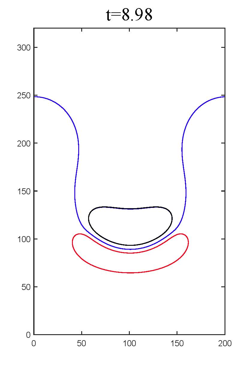
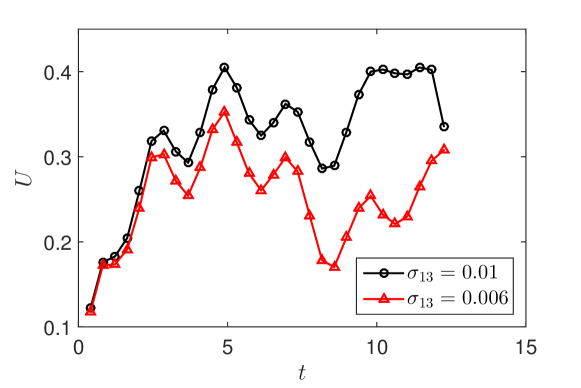
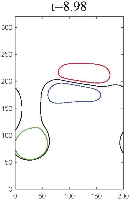
We next look into the effect of the surface tension on the fluid interfaces. Here we set the surface tension between phase 111 and phase 333 to σ13=0.006subscript𝜎130.006\sigma_{13}=0.006. Fig. 14 depicts the evolution of the fluid interfaces. One can observe that at t=8.98𝑡8.98t=8.98, the droplet (phase 111) in Fig. 14 produces a larger deformation than in Fig. 13, and in Fig. 14, phase 333 doesn’t break to form small droplets at t=12.25𝑡12.25t=12.25. To explain this, we introduce a dimensionless parameter, Bo=ΔρgD2σ13𝐵𝑜Δ𝜌𝑔superscript𝐷2subscript𝜎13Bo=\frac{\Delta\rho gD^{2}}{\sigma_{13}}, which can be used to describe the ratio of droplet gravity to surface tension. In the former case, Bo=10.8𝐵𝑜10.8Bo=10.8, while in this case, Bo=18.0𝐵𝑜18.0Bo=18.0. As the Bo𝐵𝑜Bo number increases, the gravity of the droplet is more prominent, and the droplet is more susceptible to deformation (see Fig. 14). This deformation causes the droplet to be subjected to greater resistance during the falling process, resulting in a slower drop of the droplet. As shown in Fig. 15, when σ13=0.006subscript𝜎130.006\sigma_{13}=0.006, the falling speed of the droplet U𝑈U is significantly smaller than the one when σ13=0.01subscript𝜎130.01\sigma_{13}=0.01, where U𝑈U has been normalized by U=UlgD𝑈subscript𝑈𝑙𝑔𝐷U=\frac{U_{l}}{\sqrt{gD}}, and Ulsubscript𝑈𝑙U_{l} is the velocity in the lattice unit. Eventually, a smaller drop velocity will cause the interface dynamics of this four-phase flow problem to be less complicated.
Refer to caption
Refer to caption
Refer to caption
Refer to caption
Refer to caption
Refer to caption
Figure 14: (Color online) Evolution of the fluid interfaces with σ13=0.006subscript𝜎130.006\sigma_{13}=0.006, where the time has been non-dimensionalized through t=tlDg𝑡subscript𝑡𝑙𝐷𝑔t=\frac{t_{l}}{\sqrt{\frac{D}{g}}}.
Refer to caption
Figure 15: (Color online) Comparison of the droplet front velocity with different surface tension σ13subscript𝜎13\sigma_{13}.

5.2 Dynamics of droplets and interfaces for five fluid phases

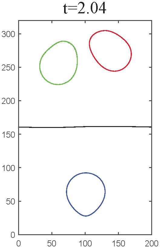
In this section, to demonstrate the ability to calculate the dynamic problem involving five fluid phases using the present model, we will consider a complex problem of droplet and interface motion involving five fluid phases. The initial setup of the physical problem is shown in Fig. 16. Similar to the previous example, the upper part of the domain is filled with phase 444, and the lower part is filled with phase 555. While in this simulation, two droplets (i.e., phase 111 and phase 222) of the same diameter are located inside phase 444, and a bubble of the same size, referred to as phase 333, is located in phase 444. Then they start moving simultaneously under gravity (buoyancy). The simulation was carried out in a uniform mesh of NY×NX=320×200𝑁𝑌𝑁𝑋320200NY\times NX=320\times 200 with periodic boundary conditions in the horizontal direction and halfway bounce-back boundary conditions in the vertical direction. The profiles of the volume fractions can be initialized by

c1(x,y)=0.5+0.5tanhR(xxc1)2+(yyc1)22η,subscript𝑐1𝑥𝑦0.50.5𝑅superscript𝑥subscript𝑥subscript𝑐12superscript𝑦subscript𝑦subscript𝑐122𝜂\displaystyle c_{1}(x,y)=0.5+0.5\tanh\frac{R-\sqrt{(x-x_{c_{1}})^{2}+(y-y_{c_{1}})^{2}}}{\sqrt{2}\eta}, (61a)
c2(x,y)=0.5+0.5tanhR(xxc2)2+(yyc2)22η,subscript𝑐2𝑥𝑦0.50.5𝑅superscript𝑥subscript𝑥subscript𝑐22superscript𝑦subscript𝑦subscript𝑐222𝜂\displaystyle c_{2}(x,y)=0.5+0.5\tanh\frac{R-\sqrt{(x-x_{c_{2}})^{2}+(y-y_{c_{2}})^{2}}}{\sqrt{2}\eta}, (61b)
c3(x,y)=0.5+0.5tanhR(xxc3)2+(yyc3)22η,subscript𝑐3𝑥𝑦0.50.5𝑅superscript𝑥subscript𝑥subscript𝑐32superscript𝑦subscript𝑦subscript𝑐322𝜂\displaystyle c_{3}(x,y)=0.5+0.5\tanh\frac{R-\sqrt{(x-x_{c_{3}})^{2}+(y-y_{c_{3}})^{2}}}{\sqrt{2}\eta}, (61c)
c5(x,y)=(0.50.5tanhyy02η)×[1.0c3(x,y)]subscript𝑐5𝑥𝑦0.50.5𝑦subscript𝑦02𝜂delimited-[]1.0subscript𝑐3𝑥𝑦\displaystyle c_{5}(x,y)=\left(0.5-0.5\tanh\frac{y-y_{0}}{\sqrt{2}\eta}\right)\times[1.0-c_{3}(x,y)] (61d)
c4(x,y)=1.0c1(x,y)c2(x,y)c3(x,y)c5(x,y),subscript𝑐4𝑥𝑦1.0subscript𝑐1𝑥𝑦subscript𝑐2𝑥𝑦subscript𝑐3𝑥𝑦subscript𝑐5𝑥𝑦\displaystyle c_{4}(x,y)=1.0-c_{1}(x,y)-c_{2}(x,y)-c_{3}(x,y)-c_{5}(x,y), (61e)

where R𝑅R is the radius of the circle drop for phase 111, 222 and 333. (xc1,yc1)subscript𝑥subscript𝑐1subscript𝑦subscript𝑐1(x_{c_{1}},y_{c_{1}}), (xc2,yc2)subscript𝑥subscript𝑐2subscript𝑦subscript𝑐2(x_{c_{2}},y_{c_{2}}) and (xc3,yc3)subscript𝑥subscript𝑐3subscript𝑦subscript𝑐3(x_{c_{3}},y_{c_{3}}) are the center of two droplets and the bubble, and y0=12NYsubscript𝑦012𝑁𝑌y_{0}=\frac{1}{2}NY is the initial surface position between phase 444 and phase 555. In this test, R=30𝑅30R=30, (xc1,yc1)=(60,280)subscript𝑥subscript𝑐1subscript𝑦subscript𝑐160280(x_{c_{1}},y_{c_{1}})=(60,280), (xc2,yc2)=(140,280)subscript𝑥subscript𝑐2subscript𝑦subscript𝑐2140280(x_{c_{2}},y_{c_{2}})=(140,280), (xc3,yc3)=(100,40)subscript𝑥subscript𝑐3subscript𝑦subscript𝑐310040(x_{c_{3}},y_{c_{3}})=(100,40). This complex five-phase problem has higher requirements for the selection of difference schemes. To further reduce the parasitic currents and guarantee the stability of present LB model, here we adopt the following isotropic mixed difference scheme [60]

ζ(𝐱,t)=i0ωi𝐜i[ζ(𝐱+2𝐜iΔt,t)+5ζ(𝐱+𝐜iΔt,t)3ζ(𝐱,t)ζ(𝐱𝐜iΔt,t)]4cs2Δt.𝜁𝐱𝑡subscript𝑖0subscript𝜔𝑖subscript𝐜𝑖delimited-[]𝜁𝐱2subscript𝐜𝑖Δ𝑡𝑡5𝜁𝐱subscript𝐜𝑖Δ𝑡𝑡3𝜁𝐱𝑡𝜁𝐱subscript𝐜𝑖Δ𝑡𝑡4superscriptsubscript𝑐𝑠2Δ𝑡\nabla\zeta(\mathbf{x},t)=\sum_{i\neq 0}\frac{\omega_{i}\mathbf{c}_{i}[\zeta(\mathbf{x}+2\mathbf{c}_{i}\Delta t,t)+5\zeta(\mathbf{x}+\mathbf{c}_{i}\Delta t,t)-3\zeta(\mathbf{x},t)-\zeta(\mathbf{x}-\mathbf{c}_{i}\Delta t,t)]}{4c_{s}^{2}\Delta t}. (62)

Although this scheme may not conserve the mass and momentum precisely due to the discretization errors [54], due to the better stability of this scheme, we will adopt this difference scheme for five-phase flows. Actually, the mass change can be controlled within 0.1%percent0.10.1\% after numerical tests, which can be ignored in the simulation. The other physical parameters in our simulations are set to be ρ1:ρ2:ρ3:ρ4:ρ5=6:4:1:2:3:subscript𝜌1subscript𝜌2:subscript𝜌3:subscript𝜌4:subscript𝜌56:4:1:2:3\rho_{1}:\rho_{2}:\rho_{3}:\rho_{4}:\rho_{5}=6:4:1:2:3, σij=0.01subscript𝜎𝑖𝑗0.01\sigma_{ij}=0.01, (1ij5)1𝑖𝑗5(1\leq i\neq j\leq 5), τg=τ1=τ2=τ3=τ4=0.8subscript𝜏𝑔subscript𝜏1subscript𝜏2subscript𝜏3subscript𝜏40.8\tau_{g}=\tau_{1}=\tau_{2}=\tau_{3}=\tau_{4}=0.8, m1=m2=m3=m4=0.1subscript𝑚1subscript𝑚2subscript𝑚3subscript𝑚40.1m_{1}=m_{2}=m_{3}=m_{4}=0.1, η=2𝜂2\eta=\sqrt{2}, β=0.06𝛽0.06\beta=\sqrt{0.06}, g=105𝑔superscript105g=10^{-5}. Fig. 17 depicts the evolution of the fluid interfaces for five fluid phases. It is found that after releasing at t=0𝑡0t=0, the two droplets of phase 111 and phase 222 fall freely in phase 444, while the bubble of phase 333 rise in phase 555. Due to the higher density, phase 111 falls faster than phase 222, and the interface between phase 444 and phase 555 begins to deform due to the movement of the droplets [see Fig. 17]. Fig. 17 shows that the droplets and the bubble approach the surface between phase 444 and 555. As time goes by, phase 111 continues to move downward, causing phase 444 to penetrate into phase 555 to form a spike [see Figs. 17 and 17]. At the same time, another droplet (phase 222) and the bubble (phase 333) are about to impact the interface between phase 444 and phase 555. At t=10.21𝑡10.21t=10.21, the droplet penetrates into phase 555 from phase 444. Meanwhile, phase 222 and phase 333 gradually become unstable, and the interface between them begins to incline to the right. Subsequently, phase 222 continues to move upward due to the buoyancy, phase 333 moves downward around phase 222, and causes a small drop of phase 444 to be trapped between phase 222 and phase 555.

Fig. 18 depicts the temporal sequence of snapshots of velocity fields at a few special moments. At t=4.08𝑡4.08t=4.08, the falling droplet of phase 111 and the bubble (phase 333) have induced a distinct velocity field. Subsequently, phase 111 moves downward, penetrating into phase 555 with a pair of vortices [see Fig. 18]. After that, the velocity field of phase 111 gradually subsides [Figs. 18 and 18]. On the other hand, phase 222 and phase 333 produce a clockwise velocity field after contact at t=12.25𝑡12.25t=12.25, eventually causing phase 222 and Phase 333 to bypass each other and then move in the opposite direction.
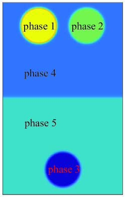
Refer to caption
Figure 16: (Color online) Initial configuration of dynamics of droplets and interfaces for five fluid phases.
Refer to caption
Refer to caption
Refer to caption
Refer to caption
Refer to caption
Refer to caption
Refer to caption
Refer to caption
Refer to caption
Figure 17: (Color online) Evolution of the fluid interfaces for five fluid phases with ρ1:ρ2:ρ3:ρ4:ρ5=6:4:1:2:3:subscript𝜌1subscript𝜌2:subscript𝜌3:subscript𝜌4:subscript𝜌56:4:1:2:3\rho_{1}:\rho_{2}:\rho_{3}:\rho_{4}:\rho_{5}=6:4:1:2:3, where the time has been non-dimensionalized through t=tlDg𝑡subscript𝑡𝑙𝐷𝑔t=\frac{t_{l}}{\sqrt{\frac{D}{g}}}.
Refer to caption
Refer to caption
Refer to caption
Refer to caption
Figure 18: (Color online) Temporal sequence of snapshots of velocity fields for five fluid phase with ρ1:ρ2:ρ3:ρ4:ρ5=6:4:1:2:3:subscript𝜌1subscript𝜌2:subscript𝜌3:subscript𝜌4:subscript𝜌56:4:1:2:3\rho_{1}:\rho_{2}:\rho_{3}:\rho_{4}:\rho_{5}=6:4:1:2:3, where the time has been non-dimensionalized through t=tlDg𝑡subscript𝑡𝑙𝐷𝑔t=\frac{t_{l}}{\sqrt{\frac{D}{g}}}.

We next investigate the effect of density ratio. In the present case, the density ratio is set to be ρ1:ρ2:ρ3:ρ4:ρ5=6:4:1:3:2:subscript𝜌1subscript𝜌2:subscript𝜌3:subscript𝜌4:subscript𝜌56:4:1:3:2\rho_{1}:\rho_{2}:\rho_{3}:\rho_{4}:\rho_{5}=6:4:1:3:2. As illustrated in Fig. 19, the current droplets and bubble (phases 111, 222 and 333) move more slowly in contrast to the previous case, because the droplets and bubble are subject to smaller gravity (buoyancy) [Figs. 19-19]. Another significant difference is that phase 222 and phase 333 bypass each other in the opposite direction to the previous example [Figs. 19-19]. This phenomenon can be observed and explained more intuitively through the velocity field at time t=12.25𝑡12.25t=12.25 [Fig. 20]. At this moment, we find that the vortex between phase 222 and phase 333 is counterclockwise in the current situation, which is the opposite of the vortex direction in the previous example. Because the density of the upper fluid (phase 444) is larger than that of the lower one (phase 555), the interface between phase 444 and phase 555 undergoes a more distinct deformation [Figs. 19-19]. Finally, phase 111 and phase 222 fall to the bottom and phase 333 rise to the top of the calculation domain.
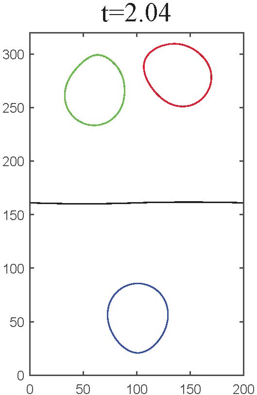
Refer to caption
Refer to caption
Refer to caption
Refer to caption
Refer to caption
Refer to caption
Refer to caption
Refer to caption
Refer to caption
Figure 19: (Color online) Evolution of the fluid interfaces for five fluid phases with ρ1:ρ2:ρ3:ρ4:ρ5=6:4:1:3:2:subscript𝜌1subscript𝜌2:subscript𝜌3:subscript𝜌4:subscript𝜌56:4:1:3:2\rho_{1}:\rho_{2}:\rho_{3}:\rho_{4}:\rho_{5}=6:4:1:3:2, where the time has been non-dimensionalized through t=tlDg𝑡subscript𝑡𝑙𝐷𝑔t=\frac{t_{l}}{\sqrt{\frac{D}{g}}}.
Refer to caption
Refer to caption
Refer to caption
Refer to caption
Figure 20: (Color online) Temporal sequence of snapshots of velocity fields for five fluid phase with ρ1:ρ2:ρ3:ρ4:ρ5=6:4:1:3:2:subscript𝜌1subscript𝜌2:subscript𝜌3:subscript𝜌4:subscript𝜌56:4:1:3:2\rho_{1}:\rho_{2}:\rho_{3}:\rho_{4}:\rho_{5}=6:4:1:3:2, where the time has been non-dimensionalized through t=tlDg𝑡subscript𝑡𝑙𝐷𝑔t=\frac{t_{l}}{\sqrt{\frac{D}{g}}}.

6 Conclusions

In this study, a LB model based on the multicomponent phase field theory is proposed for N𝑁N-phase flow systems (N2𝑁2N\geq 2). In the proposed model, we reformulate the governing equations of the N𝑁N-phase system proposed by Dong [4], and the new governing equations are also thermodynamically consistent. We point out that the velocity in this model is the volume-averaged mixture velocity and is divergence free. Besides, the mixing energy density coefficients in the free energy involve the interaction between different phases and can be determined by the pairwise surface tensions among the N fluids. In the present LB model, (N1)𝑁1(N-1) LB equations are employed to capture the interface, and another LB equation is used to solve the N-S equations. To reduce the calculation of the gradient term, a distribution function for the force term is carefully designed in the LB equation for flow field , and the governing equations can be recovered correctly through Chapmann-Enskog analysis.

The proposed model is first validated by two classical benchmark problems, including tests of static droplets and the spreading of a liquid lens, the simulation results show that the current LB model is accurate and efficient for simulating incompressible N𝑁N-phase fluid flows. To further demonstrate the capability and performance of the LB model, we use two numerical simulations, including dynamics of droplet collision for four fluid phases and dynamics of droplets and interfaces for five fluid phases, to test the proposed model. The results show that the present model can be used to handle complex interactions among multiple types of fluid interfaces.

Acknowledgements

This work is financially supported by the National Natural Science Foundation of China (Grant Nos. 51576079, 51836003), and the National Key Research and Development Program of China (Grant No. 2017YFE0100100).

Appendix A Chapman-Enskog analysis of the present model

In this appendix, the Chapman-Enskog (C-E) expansion is performed to demonstrate the consistency of the present LB model with hydrodynamic equations [Eqs. (20)].

Before performing C-E expansion, the moment conditions are first given based on the expressions of the equilibrium and force distribution functions,

kgkeq=ρ0,k𝐜kαgkeq=ρuα,k𝐜kα𝐜kβgkeq=pδαβ+ρuαuβ,k𝐜kα𝐜kβ𝐜kγgkeq=ρcs2Δαβγθuθ.\begin{split}&\sum_{k}g_{k}^{eq}=\rho_{0},\quad\sum_{k}\mathbf{c}_{k\alpha}g_{k}^{eq}=\rho u_{\alpha},\\ &\sum_{k}\mathbf{c}_{k\alpha}\mathbf{c}_{k\beta}g_{k}^{eq}=p\delta_{\alpha\beta}+\rho u_{\alpha}u_{\beta},\\ &\sum_{k}\mathbf{c}_{k\alpha}\mathbf{c}_{k\beta}\mathbf{c}_{k\gamma}g_{k}^{eq}=\rho c_{s}^{2}\Delta_{\alpha\beta\gamma\theta}u_{\theta}.\end{split} (63a)
kGk=uααρ,k𝐜kαGk=Fα,k𝐜kα𝐜kβGk=uαFβ+uβFα+cs2uαβρ+cs2uβαρ+(cs2uγγρ)δαβ+J~αuβΔt(τg0.5),\begin{split}&\sum_{k}G_{k}=u_{\alpha}\partial_{\alpha}\rho,\quad\sum_{k}\mathbf{c}_{k\alpha}G_{k}=F_{\alpha},\\ &\sum_{k}\mathbf{c}_{k\alpha}\mathbf{c}_{k\beta}G_{k}=u_{\alpha}F_{\beta}+u_{\beta}F_{\alpha}+c_{s}^{2}u_{\alpha}\partial_{\beta}\rho+c_{s}^{2}u_{\beta}\partial_{\alpha}\rho+(c_{s}^{2}u_{\gamma}\partial_{\gamma}\rho)\delta_{\alpha\beta}+\frac{\tilde{J}_{\alpha}u_{\beta}}{\Delta t(\tau_{g}-0.5)},\end{split} (63b)

where ΔαβγθsubscriptΔ𝛼𝛽𝛾𝜃\Delta_{\alpha\beta\gamma\theta} is given by Δαβγθ=δαβδγθ+δαγδβθ+δβγδαθsubscriptΔ𝛼𝛽𝛾𝜃subscript𝛿𝛼𝛽subscript𝛿𝛾𝜃subscript𝛿𝛼𝛾subscript𝛿𝛽𝜃subscript𝛿𝛽𝛾subscript𝛿𝛼𝜃\Delta_{\alpha\beta\gamma\theta}=\delta_{\alpha\beta}\delta_{\gamma\theta}+\delta_{\alpha\gamma}\delta_{\beta\theta}+\delta_{\beta\gamma}\delta_{\alpha\theta}, and Greek indices denote Cartesian spatial components.

In the C-E analysis, the time and space derivatives, as well as the force term can be expanded as

gk=gk(0)+ϵgk(1)+ϵ2gk(2)+,subscript𝑔𝑘superscriptsubscript𝑔𝑘0italic-ϵsuperscriptsubscript𝑔𝑘1superscriptitalic-ϵ2superscriptsubscript𝑔𝑘2g_{k}=g_{k}^{(0)}+\epsilon g_{k}^{(1)}+\epsilon^{2}g_{k}^{(2)}+\cdots, (64a)
Gk=ϵGk(1)+ϵ2Gk(2),subscript𝐺𝑘italic-ϵsuperscriptsubscript𝐺𝑘1superscriptitalic-ϵ2superscriptsubscript𝐺𝑘2G_{k}=\epsilon G_{k}^{(1)}+\epsilon^{2}G_{k}^{(2)}, (64b)
t=ϵt1+ϵ2t2,α=ϵ1α,formulae-sequencesubscript𝑡italic-ϵsubscriptsubscript𝑡1superscriptitalic-ϵ2subscriptsubscript𝑡2subscript𝛼italic-ϵsubscript1𝛼\partial_{t}=\epsilon\partial_{t_{1}}+\epsilon^{2}\partial_{t_{2}},\partial_{\alpha}=\epsilon\partial_{1\alpha}, (64c)
Fα=ϵFα(1)+ϵ2Fα(2),subscript𝐹𝛼italic-ϵsuperscriptsubscript𝐹𝛼1superscriptitalic-ϵ2superscriptsubscript𝐹𝛼2F_{\alpha}=\epsilon F_{\alpha}^{(1)}+\epsilon^{2}F_{\alpha}^{(2)}, (64d)

where ϵitalic-ϵ\epsilon denotes a small expansion parameter. Using the Taylor expansion to Eq. (33), one have

ΔtDkgk(x,t)+Δt22Dk2gk(x,t)+=1τg(gk(𝐱,t)gkeq(𝐱,t))+Δt(112τg)Gk,Δ𝑡subscript𝐷𝑘subscript𝑔𝑘x𝑡Δsuperscript𝑡22superscriptsubscript𝐷𝑘2subscript𝑔𝑘x𝑡1subscript𝜏𝑔subscript𝑔𝑘𝐱𝑡superscriptsubscript𝑔𝑘𝑒𝑞𝐱𝑡Δ𝑡112subscript𝜏𝑔subscript𝐺𝑘\Delta tD_{k}g_{k}(\textbf{x},t)+\frac{\Delta t^{2}}{2}D_{k}^{2}g_{k}(\textbf{x},t)+\cdots=-\frac{1}{\tau_{g}}\left(g_{k}(\mathbf{x},t)-g_{k}^{eq}(\mathbf{x},t)\right)+\Delta t(1-\frac{1}{2\tau_{g}})G_{k}, (65)

where Dk=t+ckααsubscript𝐷𝑘subscript𝑡subscript𝑐𝑘𝛼subscript𝛼D_{k}=\partial_{t}+c_{k\alpha}\partial_{\alpha}, and substituting Eq. (64d) into Eq. (65), the following multi-scale equations can be obtained,

O(ϵ0):gk(0)=gkeq,:𝑂superscriptitalic-ϵ0superscriptsubscript𝑔𝑘0superscriptsubscript𝑔𝑘𝑒𝑞O(\epsilon^{0}):g_{k}^{(0)}=g_{k}^{eq}, (66a)
O(ϵ1):D1kgk(0)=1τgΔtgk(1)+(112τg)Gk(1),:𝑂superscriptitalic-ϵ1subscript𝐷1𝑘superscriptsubscript𝑔𝑘01subscript𝜏𝑔Δ𝑡superscriptsubscript𝑔𝑘1112subscript𝜏𝑔superscriptsubscript𝐺𝑘1O(\epsilon^{1}):D_{1k}g_{k}^{(0)}=-\frac{1}{\tau_{g}\Delta t}g_{k}^{(1)}+(1-\frac{1}{2\tau_{g}})G_{k}^{(1)}, (66b)
O(ϵ2):t2gk(0)+D1kgk(1)+Δt2D1k2gk(0)=1τgΔtgk(2)+(112τg)Gk(2),:𝑂superscriptitalic-ϵ2subscriptsubscript𝑡2superscriptsubscript𝑔𝑘0subscript𝐷1𝑘superscriptsubscript𝑔𝑘1Δ𝑡2superscriptsubscript𝐷1𝑘2superscriptsubscript𝑔𝑘01subscript𝜏𝑔Δ𝑡superscriptsubscript𝑔𝑘2112subscript𝜏𝑔superscriptsubscript𝐺𝑘2O(\epsilon^{2}):\partial_{t_{2}}g_{k}^{(0)}+D_{1k}g_{k}^{(1)}+\frac{\Delta t}{2}D_{1k}^{2}g_{k}^{(0)}=-\frac{1}{\tau_{g}\Delta t}g_{k}^{(2)}+(1-\frac{1}{2\tau_{g}})G_{k}^{(2)}, (66c)

where D1k=t1+ckα1αsubscript𝐷1𝑘subscriptsubscript𝑡1subscript𝑐𝑘𝛼subscript1𝛼D_{1k}=\partial_{t_{1}}+c_{k\alpha}\partial_{1\alpha}.

Then, the substitution of Eq. (66b) into Eq. (66c) yields

t2gk(0)+(112τg)D1kgk(1)+Δt2(112τg)D1kGk(1)=1τgΔtgk(2)+(112τg)Gk(2).subscriptsubscript𝑡2superscriptsubscript𝑔𝑘0112subscript𝜏𝑔subscript𝐷1𝑘superscriptsubscript𝑔𝑘1Δ𝑡2112subscript𝜏𝑔subscript𝐷1𝑘superscriptsubscript𝐺𝑘11subscript𝜏𝑔Δ𝑡superscriptsubscript𝑔𝑘2112subscript𝜏𝑔superscriptsubscript𝐺𝑘2\partial_{t_{2}}g_{k}^{(0)}+(1-\frac{1}{2\tau_{g}})D_{1k}g_{k}^{(1)}+\frac{\Delta t}{2}(1-\frac{1}{2\tau_{g}})D_{1k}G_{k}^{(1)}=-\frac{1}{\tau_{g}\Delta t}g_{k}^{(2)}+(1-\frac{1}{2\tau_{g}})G_{k}^{(2)}. (67)

By summing Eq. (66b) and Eq. (66b)×ckβabsentsubscript𝑐𝑘𝛽\times c_{k\beta} over k𝑘k, we can obtained the recovered equations at ϵitalic-ϵ\epsilon scale,

1αρuα=1τgΔtkgk(1)+(112τg)kGk(1),subscript1𝛼𝜌subscript𝑢𝛼1subscript𝜏𝑔Δ𝑡subscript𝑘superscriptsubscript𝑔𝑘1112subscript𝜏𝑔subscript𝑘superscriptsubscript𝐺𝑘1\partial_{1\alpha}\rho u_{\alpha}=-\frac{1}{\tau_{g}\Delta t}\sum_{k}g_{k}^{(1)}+(1-\frac{1}{2\tau_{g}})\sum_{k}G_{k}^{(1)}, (68a)
t1ρuβ+1α(pδαβ+ρuαuβ)=1τgΔtkckβgk(1)+(112τg)kckβGk(1).subscriptsubscript𝑡1𝜌subscript𝑢𝛽subscript1𝛼𝑝subscript𝛿𝛼𝛽𝜌subscript𝑢𝛼subscript𝑢𝛽1subscript𝜏𝑔Δ𝑡subscript𝑘subscript𝑐𝑘𝛽superscriptsubscript𝑔𝑘1112subscript𝜏𝑔subscript𝑘subscript𝑐𝑘𝛽superscriptsubscript𝐺𝑘1\partial_{t_{1}}\rho u_{\beta}+\partial_{1\alpha}(p\delta_{\alpha\beta}+\rho u_{\alpha}u_{\beta})=-\frac{1}{\tau_{g}\Delta t}\sum_{k}c_{k\beta}g_{k}^{(1)}+(1-\frac{1}{2\tau_{g}})\sum_{k}c_{k\beta}G_{k}^{(1)}. (68b)

Similarly, the recovered equations at ϵ2superscriptitalic-ϵ2\epsilon^{2} scale can also be obtained from Eq. (67)

(112τg)[t1(kgk(1))+1α(kckαgk(1))]+Δt2(112τg)[t1(kGk(1))+1α(kckαGk(1))]=1τgΔtkgk(2)+(112τg)kGk(2),112subscript𝜏𝑔delimited-[]subscriptsubscript𝑡1subscript𝑘superscriptsubscript𝑔𝑘1subscript1𝛼subscript𝑘subscript𝑐𝑘𝛼superscriptsubscript𝑔𝑘1Δ𝑡2112subscript𝜏𝑔delimited-[]subscriptsubscript𝑡1subscript𝑘superscriptsubscript𝐺𝑘1subscript1𝛼subscript𝑘subscript𝑐𝑘𝛼superscriptsubscript𝐺𝑘11subscript𝜏𝑔Δ𝑡subscript𝑘superscriptsubscript𝑔𝑘2112subscript𝜏𝑔subscript𝑘superscriptsubscript𝐺𝑘2\begin{split}&(1-\frac{1}{2\tau_{g}})\left[\partial_{t_{1}}(\sum_{k}g_{k}^{(1)})+\partial_{1\alpha}(\sum_{k}c_{k\alpha}g_{k}^{(1)})\right]+\frac{\Delta t}{2}(1-\frac{1}{2\tau_{g}})\left[\partial_{t_{1}}(\sum_{k}G_{k}^{(1)})+\right.\\ &\left.\partial_{1\alpha}(\sum_{k}c_{k\alpha}G_{k}^{(1)})\right]=-\frac{1}{\tau_{g}\Delta t}\sum_{k}g_{k}^{(2)}+(1-\frac{1}{2\tau_{g}})\sum_{k}G_{k}^{(2)},\end{split} (69a)
t2ρuβ+(112τg)[t1(kckβgk(1))+1αΛ(1)]+Δt2(112τg)[t1(kckβGk(1))+1α(kckαckβGk(1))]=1τgΔtkckβgk(2)+(112τg)kciβGk(2),subscriptsubscript𝑡2𝜌subscript𝑢𝛽112subscript𝜏𝑔delimited-[]subscriptsubscript𝑡1subscript𝑘subscript𝑐𝑘𝛽superscriptsubscript𝑔𝑘1subscript1𝛼superscriptΛ1Δ𝑡2112subscript𝜏𝑔delimited-[]subscriptsubscript𝑡1subscript𝑘subscript𝑐𝑘𝛽superscriptsubscript𝐺𝑘1subscript1𝛼subscript𝑘subscript𝑐𝑘𝛼subscript𝑐𝑘𝛽superscriptsubscript𝐺𝑘11subscript𝜏𝑔Δ𝑡subscript𝑘subscript𝑐𝑘𝛽superscriptsubscript𝑔𝑘2112subscript𝜏𝑔subscript𝑘subscript𝑐𝑖𝛽superscriptsubscript𝐺𝑘2\begin{split}&\partial_{t_{2}}\rho u_{\beta}+(1-\frac{1}{2\tau_{g}})\left[\partial_{t_{1}}(\sum_{k}c_{k\beta}g_{k}^{(1)})+\partial_{1\alpha}\Lambda^{(1)}\right]+\frac{\Delta t}{2}(1-\frac{1}{2\tau_{g}})\left[\partial_{t_{1}}(\sum_{k}c_{k\beta}G_{k}^{(1)})+\right.\\ &\left.\partial_{1\alpha}(\sum_{k}c_{k\alpha}c_{k\beta}G_{k}^{(1)})\right]=-\frac{1}{\tau_{g}\Delta t}\sum_{k}c_{k\beta}g_{k}^{(2)}+(1-\frac{1}{2\tau_{g}})\sum_{k}c_{i\beta}G_{k}^{(2)},\end{split} (69b)

where Λ(1)=kckαckβgk(1)superscriptΛ1subscript𝑘subscript𝑐𝑘𝛼subscript𝑐𝑘𝛽superscriptsubscript𝑔𝑘1\Lambda^{(1)}=\sum_{k}c_{k\alpha}c_{k\beta}g_{k}^{(1)} is the first-order momentum flux tensor.

Summing Eq. (32) and Eq. (32)×ckαabsentsubscript𝑐𝑘𝛼\times c_{k\alpha} over k𝑘k, we can obtain the following relations

kgkeq=kgk+Δt2kGk,subscript𝑘superscriptsubscript𝑔𝑘𝑒𝑞subscript𝑘subscript𝑔𝑘Δ𝑡2subscript𝑘subscript𝐺𝑘\sum_{k}g_{k}^{eq}=\sum_{k}g_{k}+\frac{\Delta t}{2}\sum_{k}G_{k}, (70a)
kckαgkeq=kckαgk+Δt2kckαGk,subscript𝑘subscript𝑐𝑘𝛼superscriptsubscript𝑔𝑘𝑒𝑞subscript𝑘subscript𝑐𝑘𝛼subscript𝑔𝑘Δ𝑡2subscript𝑘subscript𝑐𝑘𝛼subscript𝐺𝑘\sum_{k}c_{k\alpha}g_{k}^{eq}=\sum_{k}c_{k\alpha}g_{k}+\frac{\Delta t}{2}\sum_{k}c_{k\alpha}G_{k}, (70b)

which can be further recast as

kgk(1)=Δt2kGk(1),kgk(2)=Δt2kGk(2),formulae-sequencesubscript𝑘superscriptsubscript𝑔𝑘1Δ𝑡2subscript𝑘superscriptsubscript𝐺𝑘1subscript𝑘superscriptsubscript𝑔𝑘2Δ𝑡2subscript𝑘superscriptsubscript𝐺𝑘2\sum_{k}g_{k}^{(1)}=-\frac{\Delta t}{2}\sum_{k}G_{k}^{(1)},\sum_{k}g_{k}^{(2)}=-\frac{\Delta t}{2}\sum_{k}G_{k}^{(2)}, (71a)
kckαgk(1)=Δt2kckαGk(1),kckαgk(2)=Δt2kckαGk(2).formulae-sequencesubscript𝑘subscript𝑐𝑘𝛼superscriptsubscript𝑔𝑘1Δ𝑡2subscript𝑘subscript𝑐𝑘𝛼superscriptsubscript𝐺𝑘1subscript𝑘subscript𝑐𝑘𝛼superscriptsubscript𝑔𝑘2Δ𝑡2subscript𝑘subscript𝑐𝑘𝛼superscriptsubscript𝐺𝑘2\sum_{k}c_{k\alpha}g_{k}^{(1)}=-\frac{\Delta t}{2}\sum_{k}c_{k\alpha}G_{k}^{(1)},\sum_{k}c_{k\alpha}g_{k}^{(2)}=-\frac{\Delta t}{2}\sum_{k}c_{k\alpha}G_{k}^{(2)}. (71b)

Substituting Eq. (71b) into Eqs. (68b) and (69b), one have

1αρuα=kGk(1),subscript1𝛼𝜌subscript𝑢𝛼subscript𝑘superscriptsubscript𝐺𝑘1\partial_{1\alpha}\rho u_{\alpha}=\sum_{k}G_{k}^{(1)}, (72a)
t1ρuβ+1α(pδαβ+ρuαuβ)=kckβGk(1),subscriptsubscript𝑡1𝜌subscript𝑢𝛽subscript1𝛼𝑝subscript𝛿𝛼𝛽𝜌subscript𝑢𝛼subscript𝑢𝛽subscript𝑘subscript𝑐𝑘𝛽superscriptsubscript𝐺𝑘1\partial_{t_{1}}\rho u_{\beta}+\partial_{1\alpha}(p\delta_{\alpha\beta}+\rho u_{\alpha}u_{\beta})=\sum_{k}c_{k\beta}G_{k}^{(1)}, (72b)
0=iGi(2),0subscript𝑖superscriptsubscript𝐺𝑖20=\sum_{i}G_{i}^{(2)}, (73a)
t2ρuβ+(112τg)1αΛ(1)+Δt2(112τg)1α(kckαckβGk(1))=kckβGk(2).subscriptsubscript𝑡2𝜌subscript𝑢𝛽112subscript𝜏𝑔subscript1𝛼superscriptΛ1Δ𝑡2112subscript𝜏𝑔subscript1𝛼subscript𝑘subscript𝑐𝑘𝛼subscript𝑐𝑘𝛽superscriptsubscript𝐺𝑘1subscript𝑘subscript𝑐𝑘𝛽superscriptsubscript𝐺𝑘2\partial_{t_{2}}\rho u_{\beta}+(1-\frac{1}{2\tau_{g}})\partial_{1\alpha}\Lambda^{(1)}+\frac{\Delta t}{2}(1-\frac{1}{2\tau_{g}})\partial_{1\alpha}(\sum_{k}c_{k\alpha}c_{k\beta}G_{k}^{(1)})=\sum_{k}c_{k\beta}G_{k}^{(2)}. (73b)

Combining Eq. (72a) and Eq. (73a) at ϵitalic-ϵ\epsilon and ϵ2superscriptitalic-ϵ2\epsilon^{2} scales with the help of Eqs. (63b) yields

αuα=0.subscript𝛼subscript𝑢𝛼0\partial_{\alpha}u_{\alpha}=0. (74)

To derive the equation at ϵ2superscriptitalic-ϵ2\epsilon^{2} scale, Λ(1)superscriptΛ1\Lambda^{(1)} should be expressed as

Λ(1)=τgΔt[t1kckαckβgk(0)+1γ(kckαckβckγgk(0))(112τg)kckαckβGk(1)]=τgΔt{t1pδαβ+t1(ρuαuβ)+cs21γ(ρuγδαβ)+cs21γ[ρ(uαδβγ+uβδαγ)](112τg)kckαckβGk(1)}superscriptΛ1subscript𝜏𝑔Δ𝑡delimited-[]subscriptsubscript𝑡1subscript𝑘subscript𝑐𝑘𝛼subscript𝑐𝑘𝛽superscriptsubscript𝑔𝑘0subscript1𝛾subscript𝑘subscript𝑐𝑘𝛼subscript𝑐𝑘𝛽subscript𝑐𝑘𝛾superscriptsubscript𝑔𝑘0112subscript𝜏𝑔subscript𝑘subscript𝑐𝑘𝛼subscript𝑐𝑘𝛽superscriptsubscript𝐺𝑘1subscript𝜏𝑔Δ𝑡subscriptsubscript𝑡1𝑝subscript𝛿𝛼𝛽subscriptsubscript𝑡1𝜌subscript𝑢𝛼subscript𝑢𝛽superscriptsubscript𝑐𝑠2subscript1𝛾𝜌subscript𝑢𝛾subscript𝛿𝛼𝛽superscriptsubscript𝑐𝑠2subscript1𝛾delimited-[]𝜌subscript𝑢𝛼subscript𝛿𝛽𝛾subscript𝑢𝛽subscript𝛿𝛼𝛾112subscript𝜏𝑔subscript𝑘subscript𝑐𝑘𝛼subscript𝑐𝑘𝛽superscriptsubscript𝐺𝑘1\begin{split}\Lambda^{(1)}&=-\tau_{g}\Delta t\left[\partial_{t_{1}}\sum_{k}c_{k\alpha}c_{k\beta}g_{k}^{(0)}+\partial_{1\gamma}(\sum_{k}c_{k\alpha}c_{k\beta}c_{k\gamma}g_{k}^{(0)})-(1-\frac{1}{2\tau_{g}})\sum_{k}c_{k\alpha}c_{k\beta}G_{k}^{(1)}\right]\\ &=-\tau_{g}\Delta t\left\{\partial_{t_{1}}p\delta_{\alpha\beta}+\partial_{t_{1}}(\rho u_{\alpha}u_{\beta})+c_{s}^{2}\partial_{1\gamma}(\rho u_{\gamma}\delta_{\alpha\beta})+c_{s}^{2}\partial_{1\gamma}[\rho(u_{\alpha\delta_{\beta\gamma}}+u_{\beta}\delta_{\alpha\gamma})]\right.\\ &\left.\quad-(1-\frac{1}{2\tau_{g}})\sum_{k}c_{k\alpha}c_{k\beta}G_{k}^{(1)}\right\}\\ \end{split} (75)

where Eq. (66b) has been used, and the term t1(ρuαuβ)subscriptsubscript𝑡1𝜌subscript𝑢𝛼subscript𝑢𝛽\partial_{t_{1}}(\rho u_{\alpha}u_{\beta}) can be written as

t1(ρuαuβ)=uαFβ(1)+uβFα(1)(uα1βp+uβ1αp),subscriptsubscript𝑡1𝜌subscript𝑢𝛼subscript𝑢𝛽subscript𝑢𝛼superscriptsubscript𝐹𝛽1subscript𝑢𝛽superscriptsubscript𝐹𝛼1subscript𝑢𝛼subscript1𝛽𝑝subscript𝑢𝛽subscript1𝛼𝑝\partial_{t_{1}}(\rho u_{\alpha}u_{\beta})=u_{\alpha}F_{\beta}^{(1)}+u_{\beta}F_{\alpha}^{(1)}-(u_{\alpha}\partial_{1\beta}p+u_{\beta}\partial_{1\alpha}p), (76)

where the Eqs. (72a) and Eq. (72b) are used, and the term of O(Ma3)𝑂𝑀superscript𝑎3O(Ma^{3}) has been neglected.

Combining Eq. (72b) with Eq. (73b) at ϵitalic-ϵ\epsilon and ϵ2superscriptitalic-ϵ2\epsilon^{2} scales, together with Eq. (75), Eq. (76) and Eq. (63b), we have

t(ρuβ)+α(ρuαuβ)=βp+α[ρν(αuβ+βuα)]+ϵΔt(τg0.5)α[t1pδαβ(uα1βp+uβ1αp)]α(J~αuβ)+Fβ,subscript𝑡𝜌subscript𝑢𝛽subscript𝛼𝜌subscript𝑢𝛼subscript𝑢𝛽subscript𝛽𝑝subscript𝛼delimited-[]𝜌𝜈subscript𝛼subscript𝑢𝛽subscript𝛽subscript𝑢𝛼italic-ϵΔ𝑡subscript𝜏𝑔0.5subscript𝛼delimited-[]subscriptsubscript𝑡1𝑝subscript𝛿𝛼𝛽subscript𝑢𝛼subscript1𝛽𝑝subscript𝑢𝛽subscript1𝛼𝑝subscript𝛼subscript~𝐽𝛼subscript𝑢𝛽subscript𝐹𝛽\begin{split}\partial_{t}(\rho u_{\beta})+\partial_{\alpha}(\rho u_{\alpha}u_{\beta})=&-\partial_{\beta}p+\partial_{\alpha}\left[\rho\nu(\partial_{\alpha}u_{\beta}+\partial_{\beta}u_{\alpha})\right]+\epsilon\Delta t(\tau_{g}-0.5)\partial_{\alpha}\left[\partial_{t_{1}}p\delta_{\alpha\beta}\right.\\ &\left.-(u_{\alpha}\partial_{1\beta}p+u_{\beta}\partial_{1\alpha}p)\right]-\partial_{\alpha}(\tilde{J}_{\alpha}u_{\beta})+F_{\beta},\end{split} (77)

with the relation of

ν=cs2(τg0.5)Δt.𝜈superscriptsubscript𝑐𝑠2subscript𝜏𝑔0.5Δ𝑡\nu=c_{s}^{2}(\tau_{g}-0.5)\Delta t. (78)

In the limit of a low Mach number, the dynamic pressure is assumed to be δpO(Ma2)similar-to𝛿𝑝𝑂𝑀superscript𝑎2\delta p\sim O(Ma^{2}). As a result, Eq. (77) will reduce to

t(ρuβ)+α(ρuαuβ)=βp+α[ρν(αuβ+βuα)]α(J~αuβ)+Fβ,subscript𝑡𝜌subscript𝑢𝛽subscript𝛼𝜌subscript𝑢𝛼subscript𝑢𝛽subscript𝛽𝑝subscript𝛼delimited-[]𝜌𝜈subscript𝛼subscript𝑢𝛽subscript𝛽subscript𝑢𝛼subscript𝛼subscript~𝐽𝛼subscript𝑢𝛽subscript𝐹𝛽\partial_{t}(\rho u_{\beta})+\partial_{\alpha}(\rho u_{\alpha}u_{\beta})=-\partial_{\beta}p+\partial_{\alpha}\left[\rho\nu(\partial_{\alpha}u_{\beta}+\partial_{\beta}u_{\alpha})\right]-\partial_{\alpha}(\tilde{J}_{\alpha}u_{\beta})+F_{\beta}, (79)

Thus, Eqs. (74) and (79) clearly shows that the incompressible N-S equations can be exactly recovered from the present LB model.

References

  • [1] A.S. Utada, E. Lorenceau, D.R. Link, P.D. Kaplan, H.A. Stone, D.A. Weitz, Monodisperse double emulsions generated from a microcapillary device, Science 308 (2005) 537-541.
  • [2] J. Guzowski, P. Garstecki, Droplet Clusters: Exploring the Phase Space of Soft Mesoscale Atoms, Phys. Rev. Lett. 114 (2015) 188302.
  • [3] G.I. Taylor, The formation of emulsions in definable fields of flow, Proc. R. Soc. Lond. A 146 (1934) 501-523.
  • [4] S. Dong, An efficient algorithm for incompressible N-phase flows, J. Comput. Phys, 276 (2014) 691-728.
  • [5] F. Boyer, C. Lapuerta, S. Minjeaud, B. Piar, M. Quintard, Cahn-Hilliard/Navier-Strokes model for the simulation of three-phase flows, Transp. Porous Med. 82 (2010) 463-483.
  • [6] H. Liang, B.C. Shi, Z.H. Chai, Lattice Boltzmann modeling of three-phase incompressible flows, Phys. Rev. E 93(1) (2016) 013308.
  • [7] P.C. Hohenberg, B.I. Halperin, Theory of dynamic critical phenomena, Rev. Mod. Phys. 49 (1977) 435-479.
  • [8] D. Anderson, G.B. McFadden, A. Wheeler, Diffuse-interface methods in fluid mechanics, Annu. Rev. Fluid Mech. 30 (1) (1998) 139-165.
  • [9] J. Lowengrub, L. Truskinovsky, Quasi-incompressible Cahn-Hilliard fluids and topological transitions, R. Soc. Lond. Proc. Ser. A Math. Phys. Engrg. Sci. 454 (1998) 2617-2654.
  • [10] L.-Q. Chen, Phase-field models for microstructure evolution, Annu. Rev. Mater. Res. 32 (1) (2002) 113-140.
  • [11] V. Badalassi, H. Ceniceros, S. Banerjee, Computation of multiphase systems with phase-field models, J. Comput. Phys. 190 (2) (2003) 371-397.
  • [12] J. Shen, X. Yang, Q. Wang, Mass and volume conservation in phase field models for binary fluids, Commun. Comput. Phys. 13 (2013) 1045-1065.
  • [13] H. Liang, Y. Li, J. X. Chen, and J. R. Xu. Axisymmetric lattice Boltzmann model for multiphase flows with large density ratio. Int. J. Heat Mass Transf, 2019, 130: 1189-1205.
  • [14] C. Hirt, B. Nichols, Volume of fluid (VOF) method for the dynamics of free boundaries, J. Comput. Phys. 39 (1981) 201-225.
  • [15] D. Gueyffier, J. Li, A. Nadim, R. Scardovelli, S. Zaleski, Volume-of-fluid interface tracking with smoothed surface stress methods for three-dimensional flows, J. Comput. Phys. 152 (1999) 423-456.
  • [16] S. Osher, J.A. Sethian, Fronts propagating with curvature-dependent speed: algorithms based on Hamilton-Jacobi formulations, J. Comput. Phys. 79 (1) (1988) 12-49.
  • [17] S.O. Unverdi, G. Tryggvason, A front-tracking method for viscous, incompressible, multi-fluid flows, J. Comput. Phys. 100 (1) (1992) 25-37.
  • [18] R.A. Gingold and J.J. Monaghan, Smoothed particle hydrodynamics: theory and application to non-spherical stars, Mon. Not. R. Astron. Soc. 181 (1977) 375-389.
  • [19] L.B. Lucy, A numerical approach to the testing of the fission hypothesis, Astron. J. 82 (1977) 1013-1024.
  • [20] L. Rayleigh, On the theory of surface forces II. Compressible fluids, The London, Edinburgh, and Dublin Philosophical Magazine and J. Sci. 33 (201) (1892) 209-220.
  • [21] H. Garcke, B. Nestler, B. Stoth, A multiPhase field concept: numerical simulations of moving phase boundaries and multiple junctions, SIAM J. Appl. Math. 60 (1999) 295-315.
  • [22] J. Kim, K. Kang, J. Lowengrub, Conservative multigrid methods for ternary Cahn-Hilliard systems, Commu. Math. Sci. 2 (1) (2004) 53-77.
  • [23] F. Boyer, C. Lapuerta, Study of a three component Cahn-Hilliard flow model, ESAIM: Math. Model. Numer. Anal. 40 (2006) 653-687.
  • [24] J. Kim, Phase field computations for ternary fluid flows, Comput. Methods Appl. Mech. Eng. 196 (2007) 4779-4788.
  • [25] J. Kim, A generalized continuous surface tension force formulation for phase-field models for multi-component immiscible fluid flows, Comput. Methods Appl. Mech. Engrg. 198 (2009) 3105-3112.
  • [26] F. Boyer, S. Minjeaud, Hierarchy of consistent n-component Cahn-Hilliard systems, Math. Models Methods Appl. Sci. 24 (14) (2014) 2885-2928.
  • [27] A. Lamura, G. Gonnella, J. Yeomans, A lattice Boltzmann model of ternary fluid mixtures, Europhys. Lett. 45 (3) (1999) 314-320.
  • [28] Q. Li, A.J. Wagner, Symmetric free-energy-based multicomponent lattice Boltzmann method, Phys. Rev. E 76 (2007) 036701.
  • [29] H. Chen, B.M. Boghosian, P.V. Coveney, M. Nekovee, A ternary lattice Boltzmann model for amphiphilic fluids, Proc. R. Soc. Lond. A 456 (2000) 2043-2057.
  • [30] M. Nekovee, P.V. Coveney, H. Chen, B.M. Boghosian, Lattice-Boltzmann model for interacting amphiphilic fluids, Phys. Rev. E 62 (2000) 8282-8294.
  • [31] I. Halliday, A.P. Hollis, C.M. Care, Lattice Boltzmann algorithm for continuum multicomponent flow, Phys. Rev. E 76 (2007) 026708.
  • [32] S. Leclaire, M. Reggio, J. Trepanier, Progress and investigation on lattice Boltzmann modeling of multiple immiscible fluids or components with variable density and viscosity ratios, J. Comput. Phys. 246 (2013) 318-342.
  • [33] M.Wöhrwag, C. Semprebon, A.M. Moqaddam, I. Karlin, H. Kusumaatmaja, Ternary free-energy entropic lattice Boltzmann model with a high density ratio, Phys. Rev. Lett. 120 (2018) 234501.
  • [34] Y. Yu, H.H. Liu, D. Liang, Y.H. Zhang, A versatile lattice Boltzmann model for immiscible ternary fluid flows, Phys. Fluids 31 (2019) 012108.
  • [35] Y. Shi, G. Tang, Y. Wang, Simulation of three-component fluid flows using the multiphase lattice Boltzmann flux solver, J. Comput. Phys. 314 (2016) 228-243.
  • [36] A.K. Gunstensen, D.H. Rothman, S. Zaleski, G. Zanetti, Lattice Boltzmann model of immiscible fluids, Phys. Rev. A 43 (1991) 4320-4327.
  • [37] X. Shan, H. Chen, Simulation of nonideal gases and liquid-gas phase transitions by the lattice Boltzmann equation, Phys. Rev. E 49 (1994) 2941-2948.
  • [38] M. Swift, W. Osborn, J. Yeomans, Lattice Boltzmann simulation of nonideal fluids, Phys. Rev. Lett. 75 (1995) 830.
  • [39] X. He, S. Chen, R. Zhang, A lattice Boltzmann scheme for incompressible multiphase flow and its application in simulation of Rayleigh-Taylor instability, J. Comput. Phys. 152 (1999) 642-663.
  • [40] Y. Wang, C. Shu, H. Huang, C. Teo, Multiphase lattice Boltzmann flux solver for incompressible multiphase flows with large density ratio, J. Comput. Phys. 280 (2015) 404-423.
  • [41] H. Liang, B.C. Shi, Z.L. Guo, Z.H. Chai, Phase-field-based multiple-relaxation-time lattice Boltzmann model for incompressible multiphase flows, Phys. Rev. E 89 (5) (2014) 053320.
  • [42] A. Fakhari, D. Bolster, Diffuse interface modeling of three-phase contact line dynamics on curved boundaries: A lattice Boltzmann model for large density and viscosity ratios, J. Comput. Phys. 334 (2017) 620-638.
  • [43] Z. Chai, D. Sun, H. Wang, B. Shi, A comparative study of local and nonlocal Allen-Cahn equations with mass conservation. Int. J. Heat Mass Transf. 122 (2018) 631-642.
  • [44] T. Krüger, H. Kusumaatmaja, G. Silva, O. Shardt, A. Kuzmin and E.M. Viggen, The lattice Boltzmann method, Springer International Publishing, 2017.
  • [45] Z.H. Chai, B.C. Shi, Z.L. Guo, A multiple-relaxation-time lattice Boltzmann model for general nonlinear anisotropic convection-diffusion equations, J. Sci. Comput. 69 (1) (2016) 355-390.
  • [46] S. Dong, Physical formulation and numerical algorithm for simulating N immiscible incompressible fluids involving general order parameters, J. Comput. Phys. 283 (2015) 98-128.
  • [47] S. Dong, Wall-bounded multiphase flows of N immiscible incompressible fluids: Consistency and contact-angle boundary condition. J. Comput. Phys. 338 (2017) 21-67.
  • [48] J.S. Rawlinson and B. Widom. Molecular theory of capillarity, Clarendon Press, Oxford, 1982.
  • [49] K.A. Smith, F.J. Solis, D.L. Chopp, A projection method for motion of triple junctions by level sets, Interfaces Free Bound. 4 (3) (2002) 263-276.
  • [50] L.-S. Luo, Unified theory of lattice Boltzmann models for nonideal gases, Phys. Rev. Lett. 81(8) (1998) 1618-1621.
  • [51] R. Du, B.C. Shi, A novel scheme for force term in the lattice BGK model, Int. J. Mod. Phys. C 17(07) (2006) 945-958.
  • [52] P.G. de Gennes, F. Brochard-Wyart, D. Quere, Capillarity an Wetting Phenomena, Spinger, New York, 2003.
  • [53] I. Langmuir, Oil lenses on water and the nature of monomolecular expanded films, J. Chem. Phys. 1 (1933) 756-776.
  • [54] Z.L. Guo, C.G. Zheng, B.C. Shi, Force imbalance in lattice Boltzmann equation for two-phase flows, Phys. Rev. E 83 (2011) 036707.
  • [55] J. Qian, C.K. Law, Regimes of coalescence and separation in droplet collision, J. Fluid Mech. 331 (2009) 59-80.
  • [56] H. Hinterbichler, C. Planchette, G. Brenn, Ternary drop collisions, Exp. Fluids 56 (10) (2015) 1-12.
  • [57] J.J. Huang, C. Shu, Y.T. Chew, Mobility-dependent bifurcations in capillarity-driven two-phase fluid systems by using a lattice Boltzmann phase-field model, Int. J. Numer. Meth. Fluids 60 (2009) 203-225.
  • [58] A. Fakhari, M.H. Rahimian, Phase-field modeling by the method of lattice Boltzmann equations, Phys. Rev. E 81(3) (2010) 036707.
  • [59] Z.H. Chai, T.S. Zhao, Lattice Boltzmann model for the convection-diffusion equation, Phys. Rev. E 87 (6) (2013) 063309.
  • [60] Y.Q. Zu, S. He, Phase-field-based lattice Boltzmann model for incompressible binary fluid systems with density and viscosity contrasts, Phys. Rev. E 87 (4) (2013) 043301.