KOBE-TH-19-03

5d Dirac fermion on quantum graph

Yukihiro Fujimoto^(a), Tomonori Inoue^(b), Makoto Sakamoto^(b),

Kazunori Takenaga^(c) and Inori Ueba^(b)

^(a)National Institute of Technology, Oita college,
Maki1666, Oaza, Oita 870-0152, Japan
^(b)Department of Physics, Kobe University, Kobe 657-8501, Japan
^(c)Faculty of Health Science, Kumamoto Health Science University
325 Izumi-machi, Kita-ku, Kumamoto 861-5598, Japan

In this paper, we investigate a five-dimensional Dirac fermion on a quantum graph that consists of a single vertex and $N$ loops. We find that the model possesses a rich structure of boundary conditions for wavefunctions on the quantum graph and they can be classified into $(2N+1)$ distinct categories. It is then shown that there appear degenerate four-dimensional chiral massless fermions in the four-dimensional mass spectrum. We briefly discuss how our model could naturally solve the problems of the fermion generation, the fermion mass hierarchy and the origin of the CP-violating phase.

1 Introduction

The standard model (SM) has been completed by the discovery of the Higgs boson. However, the SM still contains several mysteries and problems, which will remain to be solved. One is so-called the generation problem. The SM includes three sets of quarks and leptons, which have exactly the same quantum numbers except for the Yukawa couplings. Why nature provides the three generation of quarks and leptons is veiled. Another problem is the fermion mass hierarchy. Even though the second and the third generations of the quarks and the charged leptons are just copies of the first generation, their masses have an exponential hierarchy around $10^{5}$. The third problem is the origin of the CP violating phase in the Cabbibo-Kobayashi-Maskawa (CKM) matrix.

There are many attempts to try to solve the problems mentioned above. One of promising candidates will be higher-dimensional theory on extra dimensions. If extra dimensional models give the degeneracy of four-dimensional (4d) massless chiral fermions in 4d mass spectrum of Kaluza-Klein (KK) decomposition, the degeneracy will explain the generation of the quarks and the leptons. The fermion mass hierarchy could be resolved if the zero mode profiles are localized near some points on extra dimensions. This is because the mass matrix $m_{ij}$ between the i-th generation and the j-th one of the fermions will be of the form

$$m_{ij}=g_{Y}v\int dy\bigl{(}f^{(i)}_{0}(y)\bigr{)}^{\ast}{g^{(j)}_{0}(y)},$$ (1.1)

where $g_{Y}$ is a Yukawa coupling constant, $v$ is a vacuum expectation value of the Higgs field, $\int dy$ denotes the integral over the extra dimensions, and $f_{0}^{(i)}(y)$ ($g_{0}^{(j)}(y)$) is the profile of the i-th (j-th) generation of the 4d massless chiral fermions. Then, if $f_{0}^{(i)}(y)$ and $g_{0}^{(j)}(y)$ are localized functions on the extra dimensions, we will get a hierarchical mass matrix, which is sensitive to locations of localization [16, 17, 18, 19, 20, 21, 22]. A CP-violating phase can appear if the zero mode functions $f_{0}^{(i)}(y)$ and $g_{0}^{(j)}(y)$ are genuine complex functions, so that the mass matrix (1.1) can possess complex phases naturally [23].

In order to obtain extra dimensional models that possess the properties mentioned in the above paragraph, we investigate a five-dimensional (5d) Dirac action on a quantum graph, which consists of bonds and vertices. (For reviews of quantum graph, see [24, 25].) In this paper, we take, as a quantum graph, a rose graph consisting of one vertex and $N$ bonds, where each bond forms a loop that begins and ends at the vertex (see fig. 3).

Figure 1: Rose graph with one vertex and $N$ loops

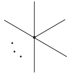
Figure 2: Star graph with one vertex and $N$ bonds

Figure 3: Interval with $(N-1)$ point interactions

One of the reason to consider the rose graph is that ordinary one-dimensional extra dimensions, like a circle or an interval, cannot solve the generation problem because no desired degeneracy appears in the spectrum. Another reason is that the rose graph with $N$ loops may be regarded as a master quantum graph with $N$ bonds because the rose graph will reduce to so-called a star graph (see fig. 3), an interval with $(N-1)$ point interactions (see fig. 3) and so on, by appropriately tuning boundary conditions (or connection conditions) for wavefunctions at the vertex of the rose graph.

In this paper, we show that allowed boundary conditions (BCs) on the rose graph can be classified into $(2N+1)$ distinct types of BCs, and clarify how many massless chiral fermions appear in the 4d mass spectrum for each type of BCs. The results show that our model possesses the desired properties mentioned in the second paragraph in this section.

The paper is organized as follows: In the next section, we give a setup of our model. In Section 3, we classify allowed boundary conditions into $(2N+1)$-types of them. In Section 4, we examine zero mode solutions for each type of the boundary conditions. In Section 5, we discuss a topological nature of the zero modes. The Section 6 is devoted to conclusion and discussion.

2 5d Dirac action on quantum graph

The 5d Dirac action we consider is given by

$$S=\int d^{4}x\sum^{N}_{a=1}\int_{L_{a-1}}^{L_{a}}dy\,\overline{\Psi}(x,y)[i\gamma^{\mu}\partial_{\mu}+i\gamma^{y}\partial_{y}{+M}]\Psi(x,y),$$ (2.1)

where $x^{\mu}$ ($\mu=0,1,2,3$) denote the coordinates of the 4d Minkowski space-time and $y$ is the coordinate of an extra dimension. $\Psi(x,y)$ is a four-component Dirac spinor on five dimensions and the Dirac conjugate $\overline{\Psi}$ is defined by $\overline{\Psi}=\Psi^{\dagger}\gamma^{0}$. $\gamma^{\mu}$ ($\mu=0,1,2,3$) are $4\times 4$ gamma matrices and $\gamma^{y}$ is taken to be $\gamma^{y}=-i\gamma^{5}$ ($\gamma^{5}=i\gamma^{0}\gamma^{1}\gamma^{2}\gamma^{3}$). $M$ is the bulk mass of the 5d Dirac fermion.

In this paper, we consider, as the extra dimension, a rose graph consisting of one vertex and $N$ bonds, each of which forms a loop with $L_{a-1}<y<L_{a}$ ($a=1,2,\cdots,N$): see fig. 4.

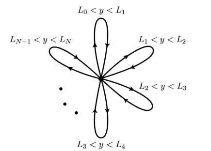
Figure 4: A rose graph consisting of one vertex and $N$ loops.

The action principle $\delta S=0$ leads to the 5d Dirac equation

$$[i\gamma^{\mu}\partial_{\mu}+i\gamma^{y}\partial_{y}{+M}]\Psi(x,y)=0,$$ (2.2)

together with

$$\sum^{N}_{a=1}\bigl{[}\overline{\Psi}(x,y)\gamma^{5}\delta\Psi(x,y)\bigr{]}^{y=L_{a}-\varepsilon}_{y=L_{a-1}+\varepsilon}=0,$$ (2.3)

where $\varepsilon$ is an infinitesimal positive constant. The condition (2.3) may be understood as the momentum conservation or the probability current conservation in the direction of the extra dimension at the center of the rose graph depicted in fig. 4. As we will see in the next section, eq. (2.3) leads to boundary conditions that the field $\Psi(x,y)$ should obey at the boundaries $y=L_{0}+\varepsilon,L_{1}\pm\varepsilon,\cdots,L_{N-1}\pm\varepsilon,L_{N}-\varepsilon$.

In terms of the 4d right-handed (left-handed) chiral spinors $\psi^{(i)}_{\textrm{R},n}(x)$ $\bigl{(}\psi^{(i)}_{{\rm L},n}(x)\bigr{)}$, the 5d Dirac spinor $\Psi(x,y)$ will be expanded into the form

$$\Psi(x,y)=\sum_{i}\sum_{n}\psi^{(i)}_{{\rm R},n}(x)f^{(i)}_{n}(y)+\sum_{i}\sum_{n}\psi^{(i)}_{{\rm L},n}(x)g^{(i)}_{n}(y),$$ (2.4)

where the index $n$ indicates the n-th level of the KK modes and i denotes the index that distinguishes the degeneracy of the n-th KK modes (if it exists). The mode functions $f^{(i)}_{n}(y)$ and $g^{(i)}_{n}(y)$ are assumed to form a complete set with respect to the extra dimensional space and satisfy the orthonormality relations

$$\sum^{N}_{a=1}\int^{L_{a}}_{L_{a-1}}dy\,\bigl{(}f^{(i)}_{n}(y)\bigr{)}^{\ast}f^{(i^{\prime})}_{n^{\prime}}(y)=\delta_{nn^{\prime}}\delta^{ii^{\prime}},$$ (2.5)

$$\sum^{N}_{a=1}\int^{L_{a}}_{L_{a-1}}dy\,\bigl{(}g^{(i)}_{n}(y)\bigr{)}^{\ast}g^{(i^{\prime})}_{n^{\prime}}(y)=\delta_{nn^{\prime}}\delta^{ii^{\prime}}.$$ (2.6)

Substituting the expansion (2.4) into eq. (2.2) and using the relations $i\gamma^{\mu}\partial_{\mu}\psi^{(i)}_{{\rm R},n}(x)+m_{n}\psi^{(i)}_{{\rm L},n}(x)=0$ and $i\gamma^{\mu}\partial_{\mu}\psi^{(i)}_{{\rm L},n}(x)+m_{n}\psi^{(i)}_{{\rm R},n}(x)=0$, which are the equations of motion for the 4d chiral spinors $\psi^{(i)}_{{{\rm R}/{\rm L}},n}(x)$ with mass $m_{n}$, we find the equations that the mode functions $f^{(i)}_{n}(y)$ and $g^{(i)}_{n}(y)$ should satisfy

$$(\partial_{y}+M)f^{(i)}_{n}(y)=m_{n}g^{(i)}_{n}(y),$$ (2.7)

$$(-\partial_{y}+M)g^{(i)}_{n}(y)=m_{n}f_{n}^{(i)}(y).$$ (2.8)

It follows that $f^{(i)}_{n}(y)$ and $g^{(i)}_{n}(y)$ satisfy the eigenvalue equations

$$(-\partial_{y}^{2}+M^{2})f^{(i)}_{n}(y)=m_{n}^{2}f^{(i)}_{n}(y),$$ (2.9)

$$(-\partial_{y}^{2}+M^{2})g^{(i)}_{n}(y)=m_{n}^{2}g^{(i)}_{n}(y).$$ (2.10)

Then, inserting the expansion (2.4) into the action (2.1), and using the relations (2.5) - (2.8), we can rewrite the action $S$, in terms of the 4d spinors, as

$$S =\int d^{4}x\Bigl{\{}\sum_{i}\overline{\psi}^{(i)}_{{\rm R},0}(x)i\gamma^{\mu}\partial_{\mu}\psi^{(i)}_{{\rm R},0}(x)+\sum_{{j}}\overline{\psi}^{({j})}_{{\rm L},0}(x)i\gamma^{\mu}\partial_{\mu}\psi^{({j})}_{{\rm L},0}(x)$$

$$\hskip 56.9055pt+\sum_{i}\sum_{n\neq 0}\overline{\psi}^{(i)}_{n}(x)(i\gamma^{\mu}{\partial_{\mu}}{+m_{n}})\psi^{(i)}_{n}(x)\Bigr{\}},$$ (2.11)

where $\psi^{(i)}_{n}(x)\equiv\psi^{(i)}_{{\rm R},n}(x)+\psi^{(i)}_{{\rm L},n}(x)$ for $n\neq 0$, and $\psi^{(i)}_{{\rm R},0}(x)$, $\psi^{(i)}_{{\rm L},0}(x)$ denote the 4d chiral massless spinors with $m_{0}=0$.

3 Classification of boundary conditions

In the previous section, we have succeeded in expressing the action $S$ in terms of the 4d mass eigenmodes. However, in order to determine the mass eigenvalue $m_{n}$ as well as the eigenfunctions $f^{(i)}_{n}(y)$ and $g^{(i)}_{n}(y)$, we need to specify some boundary conditions for the mode functions $f^{(i)}_{n}(y)$ and $g^{(i)}_{n}(y)$ at the boundaries $y=L_{0}+\varepsilon,L_{1}\pm\varepsilon,\cdots,L_{N-1}\pm\varepsilon,L_{N}-\varepsilon$. In this section, we derive allowed boundary conditions for $f^{(i)}_{n}(y)$ and $g^{(i)}_{n}(y)$ from eq. (2.3) and classify them.

Substituting the expansion (2.4) of $\Psi(x,y)$ (and also $\delta\Psi(x,y)$) into eq. (2.3) and using the fact that $\psi^{(i)}_{{\rm R}/{\rm L},n}(x)$ and $\delta\psi^{(i)}_{{\rm R}/{\rm L},n}(x)$ are independent fields, we find

$$\vec{F}^{(i)}_{n}{}^{\dagger}\vec{G}^{(j)}_{m}=\vec{G}^{(j)}_{m}{}^{\dagger}\vec{F}^{(i)}_{n}=0\qquad\text{for}\quad{}^{\forall}n,m\ \text{and}\ {{}^{\forall}i,j},$$ (3.1)

where $\vec{F}^{(i)}_{n}$ and $\vec{G}^{(j)}_{m}$ are $2N$-dimensional complex vectors defined by

$$\vec{F}^{(i)}_{n}\equiv\left(\begin{matrix}f^{(i)}_{n}(L_{0}+\varepsilon)\\ f^{(i)}_{n}(L_{1}-\varepsilon)\\ f^{(i)}_{n}(L_{1}+\varepsilon)\\ f^{(i)}_{n}(L_{2}-\varepsilon)\\ \vdots\\ f^{(i)}_{n}(L_{a-1}+\varepsilon)\\ f^{(i)}_{n}(L_{a}-\varepsilon)\\ \vdots\\ f^{(i)}_{n}(L_{N-1}+\varepsilon)\\ f^{(i)}_{n}(L_{N}-\varepsilon)\end{matrix}\right),\qquad{\vec{G}^{(j)}_{m}\equiv\left(\begin{matrix}g^{(j)}_{m}(L_{0}+\varepsilon)\\ -g^{(j)}_{m}(L_{1}-\varepsilon)\\ g^{(j)}_{m}(L_{1}+\varepsilon)\\ -g^{(j)}_{m}(L_{2}-\varepsilon)\\ \vdots\\ g^{(j)}_{m}(L_{a-1}+\varepsilon)\\ -g^{(j)}_{m}(L_{a}-\varepsilon)\\ \vdots\\ g^{(j)}_{m}(L_{N-1}+\varepsilon)\\ -g^{(j)}_{m}(L_{N}-\varepsilon)\end{matrix}\right)}.$$ (3.2)

Here, we may call $\vec{F}^{(i)}_{n}$ and $\vec{G}^{(j)}_{m}$ boundary vectors.

Let $V$ $(W)$ be the vector space spanned by $\{\vec{F}^{(i)}_{n}\}$ ($\{\vec{G}^{(j)}_{m}\}$). Then, $V$ is found to be orthogonal to $W$ in a sense of eq. (3.1) and will be regarded as the orthogonal complement space of $W$. It follows from this observation that eq. (3.1) may be replaced by the condition

$$\mathcal{P}_{-}\vec{F}^{(i)}_{n}=\mathcal{P}_{+}\vec{G}^{(j)}_{m}=0\qquad\text{for}\quad{}^{\forall}n,m\ \text{and}\ {{}^{\forall}i,j,}$$ (3.3)

where $\mathcal{P}_{\pm}$ are projection matrices that $\mathcal{P_{+}}$ ($\mathcal{P_{-}}$) maps the $2N$-dimensional complex vector space into $V$ ($W$), and they are assumed to satisfy $\mathcal{P_{+}}+\mathcal{P_{-}}=I_{2N}$ ($I_{2N}$ is the $2N\times 2N$ identity matrix), $(\mathcal{P_{\pm}})^{2}=\mathcal{P_{\pm}}$, $\mathcal{P_{+}}\mathcal{P_{-}}=\mathcal{P_{-}}\mathcal{P_{+}}=0$ and $(\mathcal{P_{\pm}})^{\dagger}=\mathcal{P_{\pm}}$.

The projection matrices $\mathcal{P_{\pm}}$ can be represented as

$$\mathcal{P_{\pm}}=\frac{1}{2}(I_{2N}\pm U),$$ (3.4)

where $U$ is a $2N\times 2N$ Hermitian matrix with the property

$$U^{2}=I_{2N}.$$ (3.5)

Thus, we found that the mode functions $f^{(i)}_{n}(y)$ and $g^{(j)}_{m}(y)$ obey the following boundary conditions

$$(I_{2N}-U)\vec{F}^{(i)}_{n}={\vec{0}},$$ (3.6)

$$(I_{2N}+U){\vec{G}^{(j)}_{m}}={\vec{0}},$$ (3.7)

for ${}^{\forall}n,m$ and ${}^{\forall}i,j$. Thus, we conclude that a Hermitian matrix $U$ satisfying eq. (3.5) specifies a 5d Dirac theory on a rose graph depicted in fig. 4.

For convenience of later analysis, we classify eqs. (3.6) and (3.7) into the $(2N+1)$ types of the boundary conditions. Since $U^{2}=I_{2N}$, the eigenvalues of $U$ are $+1$ or $-1$, so that the matrix $U$ can be classified by the number of the eigenvalue $+1$ (or $-1$). We then call the boundary condition the type ($2N-k$,$k$) if the number of the eigenvalue $+1$ ($-1$) of $U$ is $2N-k$ ($k$) for $k=0,1,2,\cdots,2N$, so that for the type ($2N-k$,$k$) BC the matrix $U$ can be expressed as

$$\text{type}\,(2N-k,k):\qquad U =V\left(\begin{array}[]{c:c}\begin{array}[]{ccc}+1&&0\\ &\ddots&\\ 0&&+1\end{array}&\begin{array}[]{ccc}{\color[rgb]{1,1,1}0}{\color[rgb]{1,1,1}0}&{\color[rgb]{1,1,1}0}\\ {\color[rgb]{1,1,1}0}&0&{\color[rgb]{1,1,1}0}\\ {\color[rgb]{1,1,1}0}&{\color[rgb]{1,1,1}0}&{\color[rgb]{1,1,1}0}\end{array}\\ \hdashline\begin{array}[]{ccc}{\color[rgb]{1,1,1}0}{\color[rgb]{1,1,1}0}&{\color[rgb]{1,1,1}0}\\ {\color[rgb]{1,1,1}0}&0&{\color[rgb]{1,1,1}0}\\ {\color[rgb]{1,1,1}0}&{\color[rgb]{1,1,1}0}&{\color[rgb]{1,1,1}0}\end{array}&\begin{array}[]{ccc}-1&&0\\ &\ddots&\\ 0&&-1\end{array}\end{array}\right)V^{\dagger},$$ (3.22)

$$\hskip 42.67912pt{\underbrace{{\color[rgb]{1,1,1}testtesttesttes}}_{2N-k}\hskip 8.5359pt\underbrace{{\color[rgb]{1,1,1}testtesttesttes}}_{k}}$$

for $V\in U(2N)$. Therefore the allowed boundary conditions on the rose graph are found to be classified into the $(2N+1)$-types of them. It follows from the form of (3.22) that the parameter space of the type ($2N-k$,$k$) BC is found to be given by the coset space $U(2N)/(U(2N-k)\times U(k))$. It should be noticed that the parameter space of the type ($2N-k$,$k$) BC is distinct from that of the type ($2N-k^{\prime}$,$k^{\prime}$) BC for $k\neq k^{\prime}$ and they are not continuously connected each other.

4 Zero mode solutions and boundary conditions

In this paper, we restrict our considerations to the zero mode solutions $f^{(i)}_{0}(y)$ and $g^{(i)}_{0}(y)$, which obey the equations (see. eqs. (2.7) and (2.8))

$$(\partial_{y}+M)f^{(i)}_{0}(y)=0,$$ (4.1)

$$(-\partial_{y}+M){g^{(j)}_{0}(y)}=0.$$ (4.2)

Any solutions to (4.1) and (4.2) will be written into the form

$$f^{(i)}_{0}(y) {=}\sum^{N}_{a=1}\theta(y-L_{a-1})\theta(L_{a}-y)A^{(i)}_{a}C_{a}e^{-My},$$ (4.3)

$$g^{(j)}_{0}(y) {=}\sum^{N}_{a=1}\theta(y-L_{a-1})\theta(L_{a}-y)B^{(j)}_{a}C^{\prime}_{a}e^{My}$$ (4.4)

for ${}^{\exists}A_{a}^{(i)},B_{a}^{(j)}\in\mathbb{C}$ ($a=1,2,\cdots,N$). The constants $C_{a}$ and $C^{\prime}_{a}$, which are independent of $i$ and $j$, will be determined later for our convenience. The coefficients $A^{(i)}_{a}$ and $B^{(j)}_{a}$ should be chosen to satisfy the boundary conditions (3.6) and (3.7). Here, $\theta(y)$ is the Heaviside step function defined as $\theta(y)=1$ for $y>0$ and $\theta(y)=0$ for $y<0$. It should be emphasized that since we are considering functions on the rose graph depicted in fig. 4, we allow the mode functions $f^{(i)}_{n}(y)$ and $g^{(i)}_{n}(y)$ to be discontinuous at the boundaries $y=L_{0},L_{1},\cdots,L_{N}$.

The indices $i$ and $j$ of $f^{(i)}_{0}(y)$ and $g^{(j)}_{0}(y)$ denote the degeneracy of the zero mode solutions. The criterion that $K$ solutions $f^{(i)}_{0}(y)$ ($i=1,2,\cdots,K$) can be independent is that the $N$-dimensional complex vectors $\mbox{\boldmath$A$}^{(i)}\equiv(A^{(i)}_{1},A^{(i)}_{2},\cdots,A^{(i)}_{N})^{\rm T}$ ($i=1,2,\cdots,K$) associated with the solutions (4.3) are linearly independent. Similarly, $K^{\prime}$ solutions $g^{(j)}_{0}(y)$ ($j=1,2,\cdots,K^{\prime}$) can be independent if the $N$ dimensional complex vectors $\mbox{\boldmath$B$}^{(j)}\equiv(B^{(j)}_{1},B^{(j)}_{2},\cdots,B^{(j)}_{N})^{\rm T}$ ($j=1,2,\cdots,K^{\prime}$) associated with the solutions (4.4) are linearly independent. The above criterion will be used later.

In the following analysis, it will be convenient to introduce the vectors $\vec{\mathcal{F}}_{a}$ and $\vec{\mathcal{G}}_{a}$ ($a=1,2,\cdots,N$) which are the $2N$-dimensional vectors defined by

$$\vec{\mathcal{F}}_{a}\equiv C_{a}(\underbrace{0,\cdots,0}_{{2(a-1)}},e^{-M(L_{a-1}+\varepsilon)},e^{-M(L_{a}-\varepsilon)},0,\cdots,0)^{\rm T},$$ (4.5)

$$\vec{\mathcal{G}}_{a}\equiv C^{\prime}_{a}(\underbrace{0,\cdots,0}_{{2(a-1)}},e^{M(L_{a-1}+\varepsilon)},-e^{M(L_{a}-\varepsilon)},0,\cdots,0)^{\rm T},$$ (4.6)

where the constants $C_{a}$ and $C^{\prime}_{a}$ ($a=1,2,\cdots,N$) are the same as those given in eqs. (4.3) and (4.4), and are chosen to be

$$\vec{\mathcal{F}}_{a}^{\dagger}\vec{\mathcal{F}}_{b}=\vec{\mathcal{G}}_{a}^{\dagger}\vec{\mathcal{G}}_{b}=\delta_{ab}\qquad(a,b=1,2,\cdots,N).$$ (4.7)

The important observations are that $\vec{\mathcal{F}}_{a}$ are orthogonal to $\vec{\mathcal{G}}_{b}$, i.e.

$$\vec{\mathcal{F}}_{a}^{\dagger}\vec{\mathcal{G}}_{b}=\vec{\mathcal{G}}_{a}^{\dagger}\vec{\mathcal{F}}_{b}=0\qquad(a,b=1,2,\cdots,N{)}$$ (4.8)

and furthermore that the set of $\{\vec{\mathcal{F}}_{a},\vec{\mathcal{G}}_{a}\ (a,b=1,2,\cdots,N)\}$ can be regarded as an orthonormal basis of the $2N$-dimensional complex vector space, so that any $2N$-dimensional complex vector can be expressed as a linear combination of $\{\vec{\mathcal{F}}_{a},\vec{\mathcal{G}}_{a}\ (a,b=1,2,\cdots,N)\}$.

In terms of $\{\vec{\mathcal{F}}_{a},\vec{\mathcal{G}}_{a}\ (a,b=1,2,\cdots,N)\}$, the boundary vectors $\vec{F}^{(i)}_{0}$ and $\vec{G}^{(j)}_{0}$ given in eq. (3.2) associated with the zero mode solutions (4.3) and (4.4) can be expressed as follows:

$$\vec{F}^{(i)}_{0}=\sum^{N}_{a=1}A_{a}^{(i)}\vec{\mathcal{F}}_{a},$$ (4.9)

$$\vec{G}^{(j)}_{0}=\sum^{N}_{a=1}B_{a}^{(j)}\vec{\mathcal{G}}_{a}.$$ (4.10)

In the following, we shall clarify how many zero mode solutions exist for each of the type ($2N-k,k$) BCs ($k=0,1,2,\cdots,2N$). This is equivalent to find linearly independent boundary vectors $\vec{F}^{(i)}_{0}$ and $\vec{G}^{(j)}_{0}$ which satisfy the boundary conditions (3.6) and (3.7) for a given $U$. To this end, it is convenient to use the fact that any $2N\times 2N$ unitary matrix $V$ can be expressed as

$$V=(\vec{u}_{1},\vec{u}_{2},\cdots,\vec{u}_{2N}),$$ (4.11)

where $\vec{u}_{p}$ ($p=1,2,\cdots,2N$) are $2N$-dimensional orthonormal complex vectors satisfying $\vec{u}_{p}{}^{\dagger}\vec{u}_{p^{\prime}}=\delta_{pp^{\prime}}$ ($p,p^{\prime}=1,2,\cdots,2N$). Then, the matrix $U$ belonging to the type ($2N-k,k$) BC will be given by

$$U=\sum^{2N-k}_{p=1}\vec{u}_{p}\vec{u}_{p}^{\dagger}-\sum^{2N}_{q=2N-k+1}\vec{u}_{q}\vec{u}_{q}^{\dagger}.$$ (4.12)

It follows that the type ($2N-k,k$) BCs, (3.6) and (3.7), reduce to

$$\vec{u}_{q}^{\dagger}\vec{F}_{0}^{(i)} =0\qquad\text{for}\quad q=2N-k+1,2N-k+2,\cdots,2N,$$ (4.13)

$$\vec{u}_{p}^{\dagger}\vec{G}_{0}^{(j)} =0\qquad\text{for}\quad p=1,2,\cdots,2N-k.$$ (4.14)

4.1 Type ($2N-k,k$) BC with $0\leq k\leq N$

Let us first consider the case of $0\leq k\leq N$. Since the set of $\{\vec{\mathcal{F}}_{a},\vec{\mathcal{G}}_{a}\ (a=1,2,\cdots,N)\}$ forms a complete set of the $2N$-dimensional complex vector space, the vectors $\{\vec{u}_{q}\,(q=2N-k+1,\cdots,2N)\}$ can be expressed as

$$\vec{u}_{q}=\sum^{N}_{a=1}\alpha_{q,{a}}\vec{\mathcal{F}}_{a}+\sum^{N}_{a=1}\beta_{q,a}\vec{\mathcal{G}}_{a}$$ (4.15)

for ${}^{\exists}\alpha_{q,a},\beta_{q,a}\in\mathbb{C}$ ($q=2N-k+1,\cdots,2N$). Inserting eqs. (4.9) and (4.15) into eq. (4.13) and using eqs. (4.7) and (4.8), we have

$$\mbox{\boldmath$\alpha$}^{\dagger}_{q}\,{\cdot}\,\mbox{\boldmath$A$}^{(i)}=0,\qquad(q=2N-k+1,\cdots,2N){,}$$ (4.16)

where $\mbox{\boldmath$\alpha$}_{q}\equiv(\alpha_{q,1},\alpha_{q,2},\cdots,\alpha_{q,N})^{{\rm T}}$.

If the maximal number of the linearly independent vectors for $\{\mbox{\boldmath$\alpha$}_{q}\,(q=2N-k+1,\cdots,2N)\}$ is $l$ with $0\leq l\leq k$, it turns out that there exist $(N-l)$ linearly independent solutions of $\mbox{\boldmath$A$}^{(i)}$ $(i=1,2,\cdots,N-l)$ to eq. (4.16). This immediately implies that there are $(N-l)$ linearly independent boundary vectors $\vec{F}^{(i)}_{0}$ $(i=1,2,\cdots,N-l)$.

In order to obtain $\vec{G}^{(j)}_{0}$, we first notice that solutions of $\vec{G}^{(j)}_{0}$ to eq. (4.14) could be written into the form

$$\vec{G}^{(j)}_{0}=\sum^{2N}_{q=2N-k+1}b^{(j)}_{q}{\vec{u}_{q}}$$ (4.17)

for ${}^{\exists}b^{(j)}_{q}\in\mathbb{C}$ ($q=2N-k+1,\cdots,2N$). Since we have assumed that the set of the vectors $\{\mbox{\boldmath$\alpha$}_{q}\,(q=2N-k+1,\cdots,2N)\}$ in eq. (4.15) consists of $l$ linearly independent vectors, by appropriately choosing the coefficients $b^{(j)}_{q}\in\mathbb{C}$ in eq. (4.17), we can obtain $(k-l)$ linearly independent solutions of the boundary vectors $\vec{G}^{(j)}_{0}$ ($j=1,2,\cdots,k-l$), which are written into the form (4.10).

Therefore, we conclude that for the type ($2N-k,k$) BC with $0\leq k\leq N$, the number of the zero mode solutions $f^{(i)}_{0}(y)$ and $g^{{(j)}}_{0}(y)$ are given as follows:

Type ($2N-k,k$) BC with $0\leq k\leq N$
             $l$              $N_{f_{0}}$              $N_{g_{0}}$              $0$              $N$              $k$              $1$              $N-1$              $k-1$              ⋮              ⋮              ⋮              $k$              $N-k$              $0$

Table 1: The number of the zero mode solutions of $f^{(i)}_{0}(y)$ and $g^{(j)}_{0}(y)$ for the type ($2N-k,k$) BC ($0\leq k\leq N$). $l$ denotes the maximal number of the linearly independent vectors $\{\mbox{\boldmath$\alpha$}_{q}\,(q=2N-k+1,\cdots,2N)\}$ in eq. (4.15). $N_{f_{0}}$ ($N_{g_{0}}$) is the number of the zero mode solutions of $f^{(i)}_{0}(y)$ ($g^{{(j)}}_{0}(y)$).

4.2 Type ($2N-k,k$) BC with $N\leq k\leq 2N$

Let us next consider the case of $N\leq k\leq 2N$. In this case, we will expand $\vec{u}_{p}$ ($p=1,2,\cdots,2N-k$) as

$$\vec{u}_{p}=\sum^{N}_{a=1}\alpha_{p,{a}}\vec{\mathcal{F}}_{a}+\sum^{N}_{a=1}\beta_{p,a}\vec{\mathcal{G}}_{a}$$ (4.18)

for ${}^{\exists}\alpha_{p,a},\beta_{p,a}\in\mathbb{C}$ ($p=1,2,\cdots,2N-k$). Inserting eqs. (4.10) and (4.18) into eq. (4.14) and using eqs. (4.7) and (4.8), we have

$${\mbox{\boldmath$\beta$}_{p}^{\dagger}}\,{\cdot}\,\mbox{\boldmath$B$}^{(j)}=0,\qquad(p=1,2,\cdots,2N-k)$$ (4.19)

where $\mbox{\boldmath$\beta$}_{p}\equiv(\beta_{p,1},\beta_{p,2},\cdots,\beta_{p,N})^{\rm T}$. If the maximal number of the linearly independent vectors for $\{\mbox{\boldmath$\beta$}_{p}\,(p=1,2,\cdots,2N-k)\}$ is $l$ with $0\leq l\leq 2N-k$, it turns out that there exist $(N-l)$ linearly independent solutions of $\mbox{\boldmath$B$}^{(j)}$ ($j=1,2,\cdots,N-l$) to eq. (4.19). This implies that there $(N-l)$ linearly independent vectors $\vec{G}^{(j)}_{0}$ ($j=1,2,\cdots,N-l$).

In order to obtain $\vec{F}^{(i)}_{0}$, we first notice that solutions of $\vec{F}^{(i)}_{0}$ to eq. (4.13) could be written into the form

$$\vec{F}^{(i)}_{0}=\sum^{2N-k}_{p=1}a_{p}^{(i)}\vec{u}_{p},$$ (4.20)

for ${}^{\exists}a^{(i)}_{p}\in\mathbb{C}$ ($p=1,2,\cdots,2N-k$). Since we have assumed that the set of the vectors $\{\mbox{\boldmath$\beta$}_{p}(p=1,2,\cdots,2N-k)\}$ in eq. (4.15) consists of $l$ linearly independent vectors, by appropriately choosing the coefficients $a^{(i)}_{p}\in\mathbb{C}$, we can obtain $(2N-k-l)$ linearly independent solutions of the boundary vectors $\vec{F}^{(i)}_{0}$ ($i=1,2,\cdots,2N-k-l$), which are written into the form (4.9).

Therefore, we conclude that for the type ($2N-k,k$) BC with $N\leq k\leq 2N$, the number of the zero mode solutions $f^{(i)}_{0}(y)$ and $g^{(j)}_{0}(y)$ are given as follows:

Type ($2N-k,k$) BC with $N\leq k\leq 2N$
             $l$              $N_{f_{0}}$              $N_{g_{0}}$              $0$              $2N-k$              $N$              $1$              $2N-k-1$              $N-1$              ⋮              ⋮              ⋮              $2N-k$              $0$              $-N+k$

Table 2: The number of the zero mode solutions of $f^{(i)}_{0}(y)$ and $g^{(j)}_{0}(y)$ for the type ($2N-k,k$) BC ($N\leq k\leq 2N$). $l$ denotes the maximal number of the linearly independent vectors $\{\mbox{\boldmath$\beta$}_{p}\,(p=1,2,\cdots,2N-k)\}$ in eq. (4.18). $N_{f_{0}}$ ($N_{g_{0}}$) is the number of the zero mode solutions of $f^{(i)}_{0}(y)$ ($g^{{(j)}}_{0}(y)$).

5 Zero mode solutions and Witten index

In the previous section, we have succeeded in finding the number $N_{f_{0}}$ ($N_{g_{0}}$) of the zero mode solutions $f^{(i)}_{0}(y)$ ($g^{{(j)}}_{0}(y)$). Then, we have seen that $N_{f_{0}}$ and $N_{g_{0}}$ depend on $l$ and $k$, where $l$ is the maximal number of linearly independent vectors for $\{\mbox{\boldmath$\alpha$}_{q}\,(q=2N-k+1,\cdots,2N)\}$ in eq. (4.15) or $\{\mbox{\boldmath$\beta$}_{p}\,(p=1,2,\cdots,2N-k)\}$ in eq. (4.18), and $k$ is the number that specifies the type ($2N-k,k$) BC. It will be worthwhile noting that the difference $\Delta_{\rm W}\equiv N_{f_{0}}-N_{g_{0}}$ is independent of $l$, i.e. $\Delta_{\rm W}=N-k$ for the type ($2N-k,k$) BC with $0\leq k\leq 2N$, though $N_{f_{0}}$ and $N_{g_{0}}$ depend on $l$ (see Table 1 and Table 2). The fact that $\Delta_{\rm W}$ is independent of $l$ is not accidental, but it has a topological reason, as we will explain below.

In the model of the 5d Dirac action on an extra dimension, a quantum-mechanical supersymmetry has been shown to be hidden in the 4d mass spectrum [39]. The Hermitian operator $H$, $Q$ and $(-1)^{F}$ defined by

$$H=Q^{2},\quad Q=\left(\begin{matrix}0&-\partial_{y}+M\\ \partial_{y}+M&0\end{matrix}\right),\quad(-1)^{F}=\left(\begin{matrix}1&0\\ 0&-1\end{matrix}\right),$$ (5.1)

are found to form a supersymmetric quantum mechanics, where $H$ is the Hamiltonian, $Q$ denotes the supercharge and $(-1)^{F}$ is called the fermion number operator. Then, the Witten index defined by

$$\Delta_{\rm W}\equiv N^{E=0}_{(-1)^{F}=+1}-N^{E=0}_{(-1)^{F}=-1}$$ (5.2)

is known to be a topological index. Here, $N^{E=0}_{(-1)^{F}=\pm 1}$ denote the numbers of the solutions with $H=0$ and $(-1)^{F}=\pm 1$, respectively. A non-trivial fact is that the supercharge $Q$ is Hermitian on the rose graph depicted in fig. 4 with the boundary conditions (3.6) and (3.7). The relations (2.7) and (2.8) for the mode functions $f^{(i)}_{n}(y)$ and $g^{(i)}_{n}(y)$ imply that they form supermultiplets for $m_{n}\neq 0$.

Since the type ($2N-k,k$) BC is not continuously connected to other ($2N-k^{\prime},k^{\prime}$) BC with $k\neq k^{\prime}$, the Witten index $\Delta_{\rm W}$ can depend on $k$ but not on $l$ because the boundary conditions with different $l$ can continuously be deformed each other.

6 Conclusion and Discussion

In this paper, we have investigated the KK decomposition of the 5d Dirac fermion on the rose graph which consists of one vertex and $N$ loops (see fig. 4). We have succeeded in classifying the allowed boundary condition on the rose graph into the type ($2N-k,k$) BC with $0\leq k\leq 2N$ and finding the number of the zero mode solutions for each type of the boundary conditions.

Our results would become phenomenologically important in constructing models beyond the standard model, based on our model considered in this paper. The chiral fermions of the standard model may correspond to the 4d chiral massless fermions $\psi^{(i)}_{{\rm R},0}(x)$ and $\psi^{(j)}_{{\rm L},0}(x)$ associated with the zero mode solutions $f^{(i)}_{0}(y)$ and $g^{(j)}_{0}(y)$. Thus, the three generation of the quarks and leptons could be obtained from a model with ${|\Delta_{\rm W}|}=3$, i.e. the type ($N-3,N+3$) BC or type ($N+3,N-3$) BC for the rose graph with $N$ loops. The fermion mass hierarchy problem in the standard model will be solved in our model because the zero mode solutions $f^{(i)}_{0}(y)$ and $g^{(j)}_{0}(y)$ are exponentially localized at some boundaries (see eqs. (4.3) and (4.4)) and the overlap integrals of zero mode solutions would produce hierarchical masses for quarks and leptons. Furthermore, our model has a natural source of a CP violating phase in the CKM matrix. This is because the boundary conditions (3.6) and (3.7) include complex parameters, in general, through the complex (Hermitian) matrix $U$, so that the zero mode solutions $f^{(i)}_{0}(y)$ and $g^{(j)}_{0}(y)$ could become genuine complex functions. Therefore, our model considered in this paper is expected to shed a new light on the generation problem, the fermion mass hierarchy and the CP-violating phase of the standard model. Phenomenological applications of our model will be reported elsewhere.

It would be of great interest to note that the rose graph depicted in fig. 4 has non-trivial geometry and that the parameter space of the boundary conditions has been found to possess a rich structure. For instance, if we take the length of all bonds to be equal ($L=L_{a}-L_{a-1}$ for $a=1,2,\cdots,N$) and choose the boundary conditions appropriately, we will have higher degeneracy in the 4d mass spectrum and then extended supersymmetries might appear in the spectrum [37, 38]. Furthermore, we will expect non-abelian Berry phases in the space of the boundary conditions with the degeneracy of the spectrum [44, 45, 46]. The issues mentioned above will be discussed in a forthcoming paper.

References

- [1] M. V. Libanov and S. V. Troitsky, “Three fermionic generations on a topological defect in extra dimensions,” Nucl. Phys. B599 (2001) 319–333, arXiv:hep-ph/0011095 [hep-ph].
- [2] J. M. Frere, M. V. Libanov, and S. V. Troitsky, “Three generations on a local vortex in extra dimensions,” Phys. Lett. B512 (2001) 169–173, arXiv:hep-ph/0012306 [hep-ph].
- [3] R. Blumenhagen, L. Goerlich, B. Kors, and D. Lust, “Noncommutative compactifications of type I strings on tori with magnetic background flux,” JHEP 10 (2000) 006, arXiv:hep-th/0007024 [hep-th].
- [4] R. Blumenhagen, B. Kors, and D. Lust, “Type I strings with F flux and B flux,” JHEP 02 (2001) 030, arXiv:hep-th/0012156 [hep-th].
- [5] D. Cremades, L. E. Ibanez, and F. Marchesano, “Computing Yukawa couplings from magnetized extra dimensions,” JHEP 05 (2004) 079, arXiv:hep-th/0404229 [hep-th].
- [6] H. Abe, T. Kobayashi, and H. Ohki, “Magnetized orbifold models,” JHEP 09 (2008) 043, arXiv:0806.4748 [hep-th].
- [7] H. Abe, K.-S. Choi, T. Kobayashi, and H. Ohki, “Three generation magnetized orbifold models,” Nucl. Phys. B814 (2009) 265–292, arXiv:0812.3534 [hep-th].
- [8] T.-H. Abe, Y. Fujimoto, T. Kobayashi, T. Miura, K. Nishiwaki, and M. Sakamoto, “ twisted orbifold models with magnetic flux,” JHEP 01 (2014) 065, arXiv:1309.4925 [hep-th].
- [9] Y. Fujimoto, T. Kobayashi, T. Miura, K. Nishiwaki, and M. Sakamoto, “Shifted orbifold models with magnetic flux,” Phys. Rev. D87 no. 8, (2013) 086001, arXiv:1302.5768 [hep-th].
- [10] T.-h. Abe, Y. Fujimoto, T. Kobayashi, T. Miura, K. Nishiwaki, and M. Sakamoto, “Operator analysis of physical states on magnetized orbifolds,” Nucl. Phys. B890 (2014) 442–480, arXiv:1409.5421 [hep-th].
- [11] T.-h. Abe, Y. Fujimoto, T. Kobayashi, T. Miura, K. Nishiwaki, M. Sakamoto, and Y. Tatsuta, “Classification of three-generation models on magnetized orbifolds,” Nucl. Phys. B894 (2015) 374–406, arXiv:1501.02787 [hep-ph].
- [12] Y. Fujimoto, K. Hasegawa, K. Nishiwaki, M. Sakamoto, and K. Tatsumi, “6d Dirac fermion on a rectangle; scrutinizing boundary conditions, mode functions and spectrum,” Nucl. Phys. B922 (2017) 186–225, arXiv:1609.01413 [hep-th].
- [13] Y. Fujimoto, K. Hasegawa, K. Nishiwaki, M. Sakamoto, and K. Tatsumi, “Supersymmetry in the 6D Dirac action,” PTEP 2017 no. 7, (2017) 073B03, arXiv:1609.04565 [hep-th].
- [14] Y. Fujimoto, K. Hasegawa, K. Nishiwaki, M. Sakamoto, K. Tatsumi, and I. Ueba, “Extended supersymmetry in Dirac action with extra dimensions,” J. Phys. A51 no. 43, (2018) 435201, arXiv:1804.02626 [hep-th].
- [15] Y. Fujimoto, K. Hasegawa, K. Nishiwaki, M. Sakamoto, K. Tatsumi, and I. Ueba, “Extended supersymmetry with central charges in higher dimensional Dirac action,” Phys. Rev. D99 no. 6, (2019) 065002, arXiv:1812.11282 [hep-th].
- [16] N. Arkani-Hamed, S. Dimopoulos, and G. R. Dvali, “The Hierarchy problem and new dimensions at a millimeter,” Phys. Lett. B429 (1998) 263–272, arXiv:hep-ph/9803315 [hep-ph].
- [17] N. Arkani-Hamed and M. Schmaltz, “Hierarchies without symmetries from extra dimensions,” Phys. Rev. D61 (2000) 033005, arXiv:hep-ph/9903417 [hep-ph].
- [18] G. R. Dvali and M. A. Shifman, “Families as neighbors in extra dimension,” Phys. Lett. B475 (2000) 295–302, arXiv:hep-ph/0001072 [hep-ph].
- [19] T. Gherghetta and A. Pomarol, “Bulk fields and supersymmetry in a slice of AdS,” Nucl. Phys. B586 (2000) 141–162, arXiv:hep-ph/0003129 [hep-ph].
- [20] S. J. Huber and Q. Shafi, “Fermion masses, mixings and proton decay in a Randall-Sundrum model,” Phys. Lett. B498 (2001) 256–262, arXiv:hep-ph/0010195 [hep-ph].
- [21] D. E. Kaplan and T. M. P. Tait, “New tools for fermion masses from extra dimensions,” JHEP 11 (2001) 051, arXiv:hep-ph/0110126 [hep-ph].
- [22] Y. Fujimoto, T. Nagasawa, S. Ohya, and M. Sakamoto, “Phase Structure of Gauge Theories on an Interval,” Prog. Theor. Phys. 126 (2011) 841–854, arXiv:1108.1976 [hep-th].
- [23] Y. Fujimoto, K. Nishiwaki, and M. Sakamoto, “CP phase from twisted Higgs vacuum expectation value in extra dimension,” Phys. Rev. D88 no. 11, (2013) 115007, arXiv:1301.7253 [hep-ph].
- [24] P. Kuchment, “Quantum graphs: I. some basic structures,” Waves in Random Media 14 no. 1, (2004) S107–S128.
- [25] P. Kuchment, “Quantum graphs: II. Some spectral properties of quantum and combinatorial graphs,” Journal of Physics A: Mathematical and General 38 no. 22, (2005) 4887–4900, arxiv:math-ph/0411003 [math-ph].
- [26] G. Berkolaiko and J. P. Keating, “Two-point spectral correlations for star graphs,” Journal of Physics A: Mathematical and General 32 no. 45, (1999) 7827–7841.
- [27] B. Bellazzini, M. Burrello, M. Mintchev, and P. Sorba, “Quantum Field Theory on Star Graphs,” Proc. Symp. Pure Math. 77 (2008) 639, arXiv:0801.2852 [hep-th].
- [28] R. Adami, C. Cacciapuoti, D. Finco, and D. Noja, “Fast solitons on star graphs,” Rev. Math. Phys. 23 (2011) 409–451, arXiv:1004.2455 [math-ph].
- [29] Y. Fujimoto, K. Konno, T. Nagasawa, and R. Takahashi, “Quantum Reflection and Transmission in Ring Systems with Double Y-Junctions: Occurrence of Perfect Reflection,” arXiv:1812.05749 [quant-ph].
- [30] S. Dimopoulos, S. Kachru, N. Kaloper, A. E. Lawrence, and E. Silverstein, “Generating small numbers by tunneling in multithroat compactifications,” Int. J. Mod. Phys. A19 (2004) 2657–2704, arXiv:hep-th/0106128 [hep-th].
- [31] H. D. Kim, “Hiding an extra dimension,” JHEP 01 (2006) 090, arXiv:hep-th/0510229 [hep-th].
- [32] G. Cacciapaglia, C. Csaki, C. Grojean, and J. Terning, “Field Theory on Multi-throat Backgrounds,” Phys. Rev. D74 (2006) 045019, arXiv:hep-ph/0604218 [hep-ph].
- [33] A. Bechinger and G. Seidl, “Resonant Dirac leptogenesis on throats,” Phys. Rev. D81 (2010) 065015, arXiv:0907.4341 [hep-ph].
- [34] S. Abel and J. Barnard, “Strong coupling, discrete symmetry and flavour,” JHEP 08 (2010) 039, arXiv:1005.1668 [hep-ph].
- [35] S. S. C. Law and K. L. McDonald, “Broken Symmetry as a Stabilizing Remnant,” Phys. Rev. D82 (2010) 104032, arXiv:1008.4336 [hep-ph].
- [36] T. Nagasawa, M. Sakamoto, and K. Takenaga, “Supersymmetry in quantum mechanics with point interactions,” Phys. Lett. B562 (2003) 358–364, arXiv:hep-th/0212192 [hep-th].
- [37] T. Nagasawa, M. Sakamoto, and K. Takenaga, “Supersymmetry and discrete transformations on with point singularities,” Phys. Lett. B583 (2004) 357–363, arXiv:hep-th/0311043 [hep-th].
- [38] T. Nagasawa, M. Sakamoto, and K. Takenaga, “Extended supersymmetry and its reduction on a circle with point singularities,” J. Phys. A38 (2005) 8053–8082, arXiv:hep-th/0505132 [hep-th].
- [39] Y. Fujimoto, T. Nagasawa, K. Nishiwaki, and M. Sakamoto, “Quark mass hierarchy and mixing via geometry of extra dimension with point interactions,” PTEP 2013 (2013) 023B07, arXiv:1209.5150 [hep-ph].
- [40] Y. Fujimoto, K. Nishiwaki, M. Sakamoto, and R. Takahashi, “Realization of lepton masses and mixing angles from point interactions in an extra dimension,” JHEP 10 (2014) 191, arXiv:1405.5872 [hep-ph].
- [41] Y. Fujimoto, T. Miura, K. Nishiwaki, and M. Sakamoto, “Dynamical generation of fermion mass hierarchy in an extra dimension,” Phys. Rev. D97 no. 11, (2018) 115039, arXiv:1709.05693 [hep-th].
- [42] V. Kostrykin and R. Schrader, “Kirchoff’s rule for quantum wires,” J. Phys. A32 (1999) 595–630.
- [43] T. Fulop and I. Tsutsui, “A Free particle on a circle with point interaction,” Phys. Lett. A264 (2000) 366, arXiv:quant-ph/9910062 [quant-ph].
- [44] F. Wilczek and A. Zee, “Appearance of Gauge Structure in Simple Dynamical Systems,” Phys. Rev. Lett. 52 (1984) 2111–2114.
- [45] S. Ohya, “Non-Abelian Monopole in the Parameter Space of Point-like Interactions,” Annals Phys. 351 (2014) 900–913, arXiv:1406.4857 [hep-th].
- [46] S. Ohya, “BPS Monopole in the Space of Boundary Conditions,” J. Phys. A48 no. 50, (2015) 505401, arXiv:1506.04738 [hep-th].