On the Structure of Liquids: More order than expected

Abstract

Disordered systems like liquids, gels, glasses, or granular materials are not only ubiquitous in daily life and in industrial applications but they are also crucial for the mechanical stability of cells or the transport of chemical and biological agents in living organisms [1, 2, 3]. Despite the importance of these systems, their microscopic structure is understood only on a rudimentary level, thus in stark contrast to the case of gases and crystals [1, 4]. Experimental and theoretical investigations indicate that disordered systems have a structural order on the length scale of a few particle diameters but which then quickly vanishes at larger distances [5]. This conclusion is, however, based mainly on the behavior of two-point correlation functions such as the static structure factor or the radial distribution function [5, 6]. Whether or not disordered systems have an order that extents to larger length scales is therefore a highly important question that is still open [7, 8, 9, 10]. Here we use computer simulations to show that liquids have an intricate structural order given by alternating layers with icosahedral and dodecahedral symmetries and which extends to surprisingly large distances. We show that the temperature dependence of the corresponding length scale can be detected in the static structure factor, making it directly accessible to scattering experiments. These results, obtained by a novel type of four point correlation function that probes directly the particle density in three dimensions, show that liquids are far more ordered than envisaged so far but that this structural information is encoded in non-standard correlation functions.

The structure of complex systems is usually determined from scattering experiments which give access to the static structure factor $S(\vec{q})$, $\vec{q}$ is the wave-vector, and for crystals such measurements allow to obtain a complete knowledge of the structure of the material [5, 6, 4]. This is not the case for disordered materials since these are isotropic and hence $S(\vec{q})$ depends only on the norm $q=|\vec{q}|$, i.e., the whole three dimensional structural information is projected onto a single function $S(q)$. This projection entails a huge loss of structural information, which subsequently has to be recovered, at least partially, from physical arguments on the possible arrangement of the particles. Since for intermediate and large length scales no such arguments exist, our current knowledge about the packing of the particles is restricted to length scales of 2-3 particle diameters [13, 16, 17, 14, 18, 8, 15, 12, 11, 7] whereas there is very little insight regarding the structure on larger scales.

Whether or not disordered systems have indeed a structural order that extents beyond a few particle diameters is one of the central questions of glass science since various theoretical approaches connect the slowing down of the relaxation dynamics to the presence of an increasing static length scale [1, 10, 20, 19], although this mechanism is challenged by other theories [21]. As a consequence there have been a multitude of proposals regarding the nature and definition of such a growing length, but so far no consensus has emerged regarding the best choice, notably in the generic case of multi-component systems [10, 12, 11, 7, 22, 23]. In the present work we use a novel approach to reveal that liquids do have highly non-trivial correlations up to distances well beyond the first few neighbors.

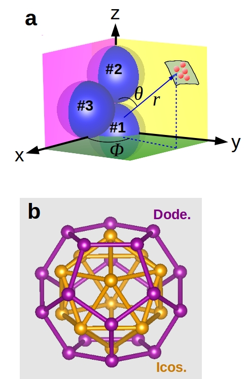
The system we consider is a binary mixture of Lennard-Jones particles (80% A particles and 20% B particles) that is not prone to crystallization even at low temperatures (see Methods) [24]. We study the equilibrium properties of this liquid in a temperature range in which the system changes from a very fluid state to a moderately viscous one, i.e. $5.0\geq T\geq 0.40$. To probe the three dimensional structure of the system we introduce a local coordinate system as follows: Take any three A particles that touch each other, i.e., they form a triangle with sides that are less than the location of the first minimum in the radial distribution function $g(r)$, i.e.$\approx 1.4$ (see Extended Data Fig. 1). We define the position of particle #1 as the origin, the direction from particle #1 to #2 as the $z-$axis, and the plane containing the three particles as the $z-x-$plane (Fig. 1a). This local reference frame allows to introduce a spherical coordinate system $\theta,\phi,r$ and to measure the probability of finding any other particle at a given point in space, i.e. to measure a four point correlation function. Note that this coordinate system can be defined for all triplets of neighboring particles and these density distributions can be averaged to improve the statistics. Since this coordinate system is adapted to the configuration by the three particles it allows to detect angular correlations that are not visible in $g(r)$ or in previously considered structural observables.

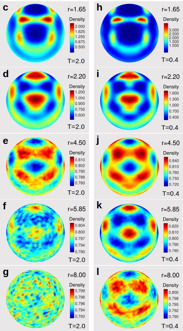
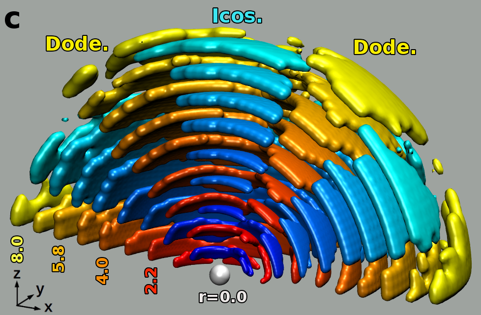
Figure 1c-l shows the three dimensional normalized distribution $\rho(\theta,\phi,r)$ of the particles on the sphere of radius $r$ centered at a particle #1. We recognize that $\rho(\theta,\phi,r)$ has a noticeable angular dependence not only at small distances but also at intermediate ones, e.g. at $r=4.5$, and at low $T$ even at large ones, e.g., $r=8.0$ (Fig. 1l), demonstrating that the liquid has a non-trivial structural order that extents to distances that are well beyond the first few neighbor shells. Furthermore one notes that $\rho(\theta,\phi,r)$ has a highly symmetric shape: For distances $r\approx 1$, i.e., the first nearest neighbor shell, one finds the expected icosahedral symmetry [13, 15], see Extended Data Fig. 2. For $r=1.65$ (Fig. 2, c and h), corresponding to the distance between the first minimum and the second nearest neighbor peak in $g(r)$, one observes a dodecahedral-like symmetry. This result can be understood by recalling that a dodecahedron is the dual of an icosahedron, and vice versa (Fig. 1b) and hence the local dip formed by three neighboring particles in the first shell will be occupied by particles forming part of the second shell, thus giving rise to a dodecahedral symmetry. The fact that this “duality mechanism” works even at large distances, see below, is surprising since it contradicts the standard view that in liquids correlations are quickly washed out at large distances. We emphasize that for geometrical reasons at large $r$ a region with high $\rho(\theta,\phi,r)$ is not a single particle, but a structure that grows linearly with $r$ and hence is a whole collection of particles, i.e., for fixed $r$ the structure is given by patches with a high density of particles that alternate with patches with low density.

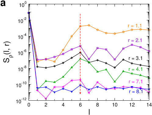
The standard way to characterize in a quantitative manner the density distribution on a sphere is to decompose it into spherical harmonics $Y_{l}^{m}$, $\rho(\theta,\phi,r)=$$\sum_{l=0}^{\infty}\sum_{m=-l}^{l}\rho_{l}^{m}(r)Y_{l}^{m}(\theta,\phi)$, where the expansion coefficients $\rho_{l}^{m}$ are given in the Methods, and to consider the angular power spectrum $S_{\rho}(l,r)=(2l+1)^{-1}\sum_{m=-l}^{l}|\rho_{l}^{m}(r)|^{2}$. For this system the component with $l=6$ is the most prominent one (Extended Data Fig. 3a), independent of $r$, a result that is reasonable in view of the icosahedral and dodecahedral symmetries that we find in the density distribution. (For systems like SiO₂ which have a local tetrahedral symmetry the relevant index is instead $l=3$.) We emphasize, however, that the results presented below do not change qualitatively if another value of $l$ is considered (Extended Data Fig. 3b).

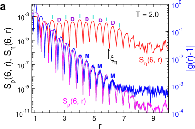
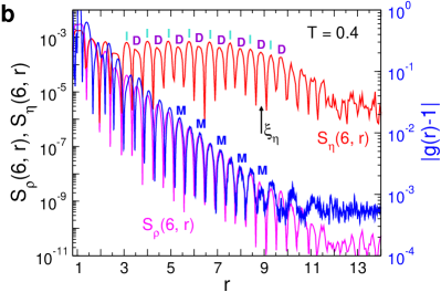
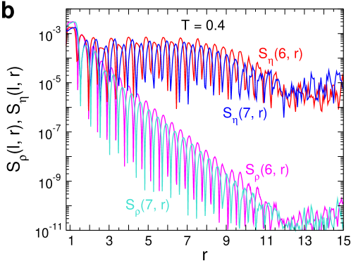
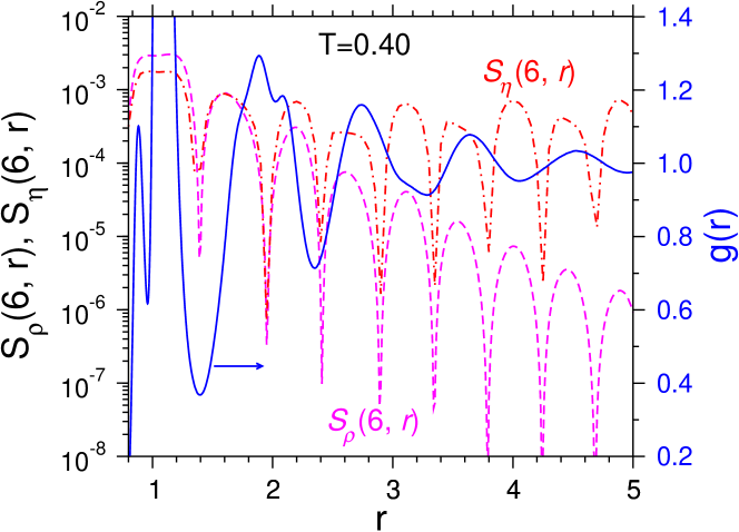
In Fig. 2 we show the $r-$dependence of $S_{\rho}(6,r)$ at a high and low temperature and one sees that the signal decays quickly with increasing $r$. Figure 1k shows that for the distance $r=5.85$ the density distribution has a pronounced structure although Fig. 2b shows that at this $r$ the absolute value of $S_{\rho}(l,r)$ is small. This smallness is due to the fact that $S_{\rho}(l,r)$ is not only sensitive to the angular dependence of the distribution, but also to the amplitude of the signal. In order to probe the symmetry properties of the density distribution it is therefore useful to consider a normalized density distribution $\eta(\theta,\phi,r)=[\rho(\theta,\phi,r)-\rho_{\rm min}(r)]/[\rho_{\rm max}(r)-\rho_{\rm min}(r)]$, where $\rho_{\rm max}(r)$ and $\rho_{\rm min}(r)$ are the maximum and minimum of $\rho(\theta,\phi,r)$, respectively. The angular power spectrum of $\eta(\theta,\phi,r)$, $S_{\eta}(r)$, is included in Fig. 2a/b as well and we see that this quantity oscillates around a constant value which shows that the density distribution has a pronounced angular dependence even at intermediate distances. For distances larger than a threshold $\xi_{\eta}(T)$, $S_{\eta}(r)$ starts to decay before it reaches at large $r$ a value that is determined by the noise of the data and below we will discuss the $T-$dependence of $\xi_{\eta}(T)$. (See Methods for a precise definition of $\xi_{\eta}$.)

Most remarkable is the observation that for distances larger than $r\approx 2.0$ the height of the local maxima in $S_{\eta}(r)$ shows a periodic behavior in that a high maximum is followed by a low one. A visual inspection of $\rho(\theta,\phi,r)$ reveals that these high/low maxima correspond to distances at which the distribution has an icosahedral/dodecahedral symmetry demonstrating that these two geometries are not only present at short distances but also at large ones, in agreement with the snapshots in Fig. 1. One thus concludes that the distribution of the particles in three dimensions is given by shells in which the particles are arranged in a pattern with alternating icosahedral/dodecahedral symmetry, see Fig. 2c. For distances larger that $r\approx 4$ one finds that the radial position of these two geometrical arrangements match well the locations of the minima/maxima in $g(r)$ (Fig. 2, a and b). This observation can be rationalized by the fact that a dodecahedron has 20 vertices (i.e., regions in which $\rho(\theta,\phi,r)$ has high values) and an icosahedron only 12, thus making that the former structure corresponds to the maxima of $g(r)$ and the latter to the minima. In contrast to this one finds no noticeable correspondence between the peaks in $S_{\eta}(r)$ and $g(r)$ for $r<3$, see also Extended Data Fig. 4, indicating that the packing in the first few shells around the central particle has not just a pure icosahedral or dodecahedral symmetry but a more complex structure that is determined by steric and energetic considerations, a result that is in agreement with previous studies of similar systems that have probed the geometry of the packing on small length scales [11, 8, 16, 17].

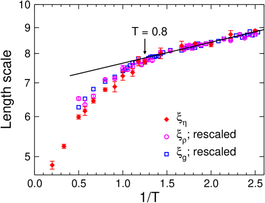
The distance $\xi_{\eta}(T)$ at which $S_{\eta}(r)$ starts to drop, see Fig. 2a/b, corresponds to a static correlation length (Extended Data Fig. 5). Figure 3 shows $\xi_{\eta}$ as a function of inverse temperature and one recognizes that this length increases by about a factor of two in the $T-$range considered. Also included in the graph are the length scales $\xi_{\rho}$ and $\xi_{g}$ that are related to the exponential decay of $S_{\rho}(r)$ and $|g(r)-1|$, respectively, see Fig. 2a/b. (See the Methods and Extended Data Fig. 5 on how to determine $\xi_{\rho}$ and $\xi_{g}$.) From the graph one recognizes two regimes: At high $T$ the length scales increase quickly with decreasing $T$ whereas at low temperatures one finds a weaker $T-$dependence and which is compatible with $\ln(\xi)\propto T^{-1}$. Hence one concludes that a decreasing temperature leads to an increasing static length scale, in agreement with previous studies that have documented a weak increase of static length scales in glass-forming systems, Ref. [10] and references therein. Surprisingly the crossover between the two regimes occurs at around $T=0.8$, thus very close to the so-called “onset temperature” $T_{\rm o}$ [24] at which the relaxation dynamics of the system crosses over from a normal dynamics to a glassy one [1]. This result shows that the change in the dynamical properties of the system has a counterpart in the statics, giving hence support to the idea that the latter allows to understand the former [25].

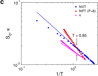
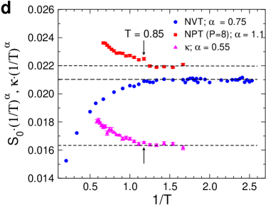
Since the $T$-dependence of $\xi_{g}$ is very similar to the one of $\xi_{\eta}$, Fig. 3, one can expect that also the intensity of the static structure factor $S(q)$ at small wave-vectors has the same $T-$dependence. Extended Data Fig. 6d shows that this is indeed the case (and the same conclusion is reached for the compressibility) which thus makes this $T-$dependence accessible to standard scattering experiments, i.e., a careful measurement of the structure factor allows to determine the $T$-dependence of the length scale $\xi_{\eta}$ as well as the onset temperature in a direct manner, i.e., without referring to any probe of the dynamics.

In conclusion we have demonstrated that liquids have a non-trivial structural correlation that extents to distances well beyond the first few nearest neighbors. This result has been obtained by using a novel method to analyze the particle coordinates and which can thus be applied to any other disordered system for which the particle coordinates are accessible, such as colloidal and granular systems, or materials in which some of the particles have been marked by fluorescence techniques [18, 26, 27, 28, 29]. Our finding that disordered systems can have anisotropic structural order extending to large length scales should trigger the improvement of experimental techniques that probe this order.

Methods

System and simulations. The system we study is a 80:20 mixture of Lennard-Jones particles (type A and B) with interactions given by $V_{\alpha\beta}(r)=4\epsilon_{\alpha\beta}[(\sigma_{\alpha\beta}/r)^{12}-(\sigma_{\alpha\beta}/r)^{6}]$, where $\alpha,\beta\in\{A,B\}$, $\sigma_{AA}=1.0$, $\epsilon_{AA}=1.0$, $\sigma_{AB}=0.8$, $\epsilon_{AB}=1.5$, $\sigma_{BB}=0.88$, and $\epsilon_{BB}=0.5$ [24]. Here we use $\sigma_{AA}$ and $\epsilon_{AA}$ as the units of length and energy, respectively. We set the mass of all particles equal to $m=1.0$ and the Boltzmann constant is $k_{B}=1.0$. Using the LAMMPS software ³⁰ we simulate a total of $10^{5}$ particles at constant volume (box size 43.68) and temperature. At the lowest temperature, $T=0.40$, the run was $1.4\cdot 10^{8}$ time steps (step size 0.005) for equilibration and the same length for production, time spans that are sufficiently large to completely equilibrate the system. For the analysis of the data we used 4 and 20 configuration for $S_{\rho}$ and $g(r)$, respectively.

Angular power spectrum. The coefficient $\rho_{l}^{m}$ for the expansion of the density distribution into spherical harmonics is given by

$$\rho_{l}^{m}=\int_{0}^{2\pi}d\phi\int_{0}^{\pi}d\theta\sin\theta\rho(\theta,\phi,r)Y_{l}^{m*}(\theta,\phi)\quad,$$

where $Y_{l}^{m*}$ is the complex conjugate of the spherical harmonic function of degree $l$ and order $m$. In practice this integration was done by sampling the integrand over up to $2\cdot 10^{9}$ points for each shell of width 0.4.

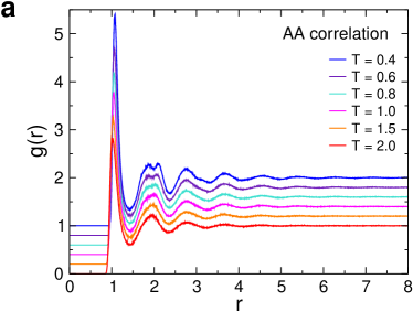
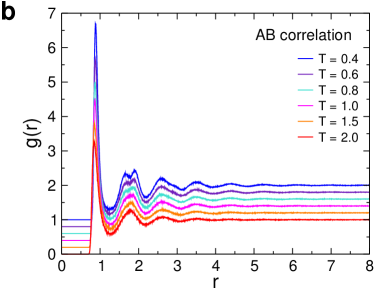
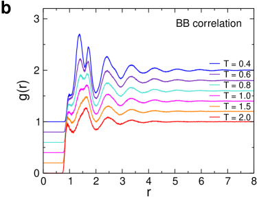
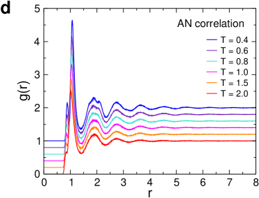
Radial distribution functions. In Extended Data Fig. 1 we show the three partial radial distribution functions $g(r)$ as well as the correlation function between an A particle and any other particle (AN). The curves correspond to different temperatures (see legend). These graphs show that the $T-$dependence of $g(r)$ is very smooth, as expected for a system that is a good glass-former.

Three dimensional distribution of the particles in the nearest neighbor shell. In Fig. 1 of the main text we show the angular distribution of the particle density for intermediate and large distances $r$. In Extended Data Fig. 2 we present this distribution for a distance that corresponds to the first coordination shell of the central particle. This graph clearly shows that this first shell has an icosahedral-like symmetry, as expected for a hard-sphere like simple liquid.

$l-$dependence of the angular power spectrum. In the main text we focus on the results for the index $l=6$ in the expansion of the spherical harmonics of the density distribution. In Extended Data Fig. 3a we show the $l-$dependence of the angular power spectrum $S_{\rho}(l,r)$ for selected distances $r$. From this graph one recognizes that for $l=6$ the signal is relatively strong for all distances and hence this value for the index is a good choice for probing the structural order in the liquid. However, as mentioned in the main text, the presented results do not depend in a crucial manner on the choice of $l$. This is demonstrated in Extended Data Fig. 3b where we compare the $r-$dependence of $S_{\rho}$ and $S_{\eta}$ for $l=7$ with the ones for $l=6$, i.e., the data shown in the main text. This figure clearly demonstrates that the $r-$dependence of the two quantities does not depend in a significant manner on $l$. (The main difference is that the signal for $l=7$ is somewhat smaller than the one for $l=6$, a result that is directly related to the fact that in this system the particles are arranged in shells with a pronounced icosahedral and dodecahedral symmetry and that these two structures have a relatively strong $l=6$ component in the angular power spectrum.) Therefore the corresponding length scales (see Fig. 3 in the main text), the radial distribution function, as well as the signal of the static structure factor at small wave-vector will all show a similar dependence on temperature (see also Extended Data Fig. 6 below).

Angular power spectra and radial distribution function at short distances. In Fig. 2 of the main text we have shown how the angular power spectra $S_{\rho}(r)$ and $S_{\eta}(r)$ and the radial distribution function $g(r)$ depend on the distance $r$. In Extended Data Fig. 4 we show these functions at small distances, i.e., $r<5.0$. One recognizes from this graph that at these small distances, in particular for $r<3.0$, the $r-$dependence is rather complex due to the local packing effects of the particles. Only for distances larger than around 4.0 the $r-$dependence of the three functions becomes regular in that the shape of the various peaks becomes independent of $r$. Thus this distance indicates the crossover between a structure at small $r$ that is determined by local packing effects to a structure at large $r$ that is determined by symmetry considerations. This symmetry at large $r$ is in turn determined by the packing at small r, i.e., in our case the icosahedra-like structure.

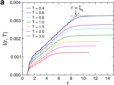
Extracting length scales. From Fig. 2a/b of the main text one recognizes that the distance $\xi_{\eta}$ at which $S_{\eta}(r,T)$ starts to drop increases if $T$ is lowered. To determine $\xi_{\eta}$ we have calculated the integral $I(r,T)=\int_{0}^{r}S_{\eta}(r^{\prime},T)dr^{\prime}$ and in Extended Data Fig. 5a we plot this quantity as a function of $r$. For small and intermediate $r$ the integral shows a basically linear increase with $r$, because the integrand $S_{\eta}(r)$ is essentially a constant, and once $S_{\eta}(r)$ starts to decay $I(r,T)$ becomes a constant. Using a fit with two straight lines this cross-over point can be determined accurately, see dashed lines in Extended Data Fig. 5a, giving thus $\xi_{\eta}(T)$.

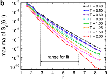
In Fig. 2a/b of the main text we have shown that $S_{\rho}(r)$ shows at intermediate and large distances an exponential dependence on the distance $r$. In Extended Data Fig. 5b we show the $r-$dependence of $S_{\rho}$ for different temperatures. Note that we plot only the local maxima of the function since these have been used to fit the data at intermediate and large distances with an exponential function (see below). From the graph one recognizes that the slope of the curves decreases with decreasing temperature, indicating that the associated length scale increases. 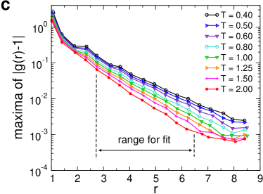We obtain this length scale $\xi_{\rho}$ by making a fit with an exponential of the form $S_{\rho}(r,T)\propto\exp(-r/\xi_{\rho}(T))$ and plot this quantity in Fig. 3 of the main text. In Extended Data Fig. 5c we show the $r-$dependence of $|g(r)-1|$ for various temperatures. (Again only the location of the maxima are shown.) We see that also this dependence can be fitted well by an exponential function, thus allowing to define a length scale $\xi_{g}(T)$, the $T-$dependence of which is included in Fig. 3 of the main text as well.

Structure factor and compressibility. The static structure factor of the system was determined directly from the positions of the particles, i.e.,

$$S({\vec{q}})=\frac{1}{N}\sum_{j=1}^{N}\sum_{k=1}^{N}\exp[{i\vec{q}}\cdot({\vec{r}}_{j}-{\vec{r}}_{k})]\quad.$$ (1)

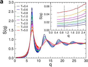
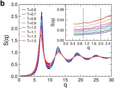
Since the system is isotropic, we have averaged $S({\vec{q}})$ over all wave-vectors ${\vec{q}}$ that have the same norm $q=|{\vec{q}}|$. In Extended Data Fig. 6a we show the $q-$dependence of $S(q)$ for different temperatures. Because of the finite size of the box, the smallest accessible wave-vector is $q=2\pi/43.68\approx 0.144$ and one has only three independent wave-vectors with this modulus. In order to estimate with good accuracy the $T-$dependence of $S(q)$ at small wave-vectors we have therefore averaged $S(q)$ over the range $1.0\leq q\leq 2.0$. This interval is shown in Extended Data Fig. 6a as well (Inset). The so obtained averaged data for $S(q)$, denoted by $S_{0}(T)$, is shown in Extended Data Fig. 6c (blue circles). In Fig. 3 of the main text we have found that the various length scales show at around $T=0.8$ a crossover in their temperature dependence. Since this crossover is seen also in the $T-$dependence of the slope of $|g(r)-1|$, one expects it to be present also in $S(q)$ at small $q$ and hence in $S_{0}(T)$. Extended Data Fig. 6c includes also a power-law fit to the low temperature data (solid blue line). (At this stage this functional form should be considered just as a parameterization of the data since we do not have a theoretical basis for it.) In order to see better the $T-$range in which this fit works well, we show in Extended Data Fig. 6d the ratio between $S_{0}$ and this power-law. One recognizes that this ratio shows an appreciable $T-$dependence for $T\geq 0.85$, but then becomes flat, i.e. the quantity $S_{0}$ does indeed show a crossover at around the onset temperature $T_{\rm o}\approx 0.8$. This result is thus coherent with the data shown in Fig. 3 of the main text and hence we can conclude that at the onset temperature the static structure of the system on large scales is indeed changing its temperature dependence.

Furthermore we mention that we have also studied the temperature dependence of $S_{0}(T)$ in the constant pressure ensemble. The chosen pressure was $P=8.0$ since this corresponds to the pressure at the onset temperature in the constant volume ensemble and hence it can be expected that the onset temperature in the two ensemble are very similar. The resulting static structure factor is presented in Extended Data Fig. 6b and the so obtained $S_{0}(T)$ is included in Extended Data Fig. 6c as well (red squares). The data at low $T$ can again be fitted well by a power-law (solid red line) and the resulting ratio between data and power-law, plotted in Extended Data Fig. 6d, shows again around $T=0.8$ a change in its temperature dependence. This result demonstrates that the $T-$dependence of the large scale structure shows at the onset temperature a marked change which is independent of the considered ensemble.

For the simulations at constant pressure we have determined also the compressibility $\kappa=(\Delta V)^{2}/(k_{B}TV)$, where $(\Delta V)^{2}$ is the variance of the volume fluctuation. In Extended Data Fig. 6c we present thus also $\kappa(T)$ and we recognize that this quantity shows a similar temperature dependence as $S_{0}$, as expected. Also in this case we find that the data at low $T$ can be described very well by a power-law (solid magenta line). In Extended Data Fig. 6d we show this in an explicit manner and one sees that the description with the power-law starts to break down at around $T=0.85$, i.e., the same temperature at which $S_{0}$ starts to deviate from the power-law. Thus one can conclude that also a careful measurement of the compressibility does allow to estimate the onset temperature $T_{\rm o}$ with good accuracy, or in other words, this temperature that is usually obtained from dynamic data can be extracted also from high precision static data.

Anisotropic radial distribution function. In Fig. 2 of the main text and Extended Data Fig. 1 we have presented the standard radial distribution function $g(r)$, i.e., the density distribution averaged over the sphere with radius $r$. Since we find that the distribution of the particles around a central particle is anisotropic it is of interest to consider also the radial distribution functions in which one probes the correlations in a specific direction with respect to the local coordinate system, Fig. 1a. We have done this analysis for the directions that correspond to the vertices of the icosahedra and of the dodecahedra, thus defining $g_{I}(r)$ and $g_{D}(r)$, respectively. 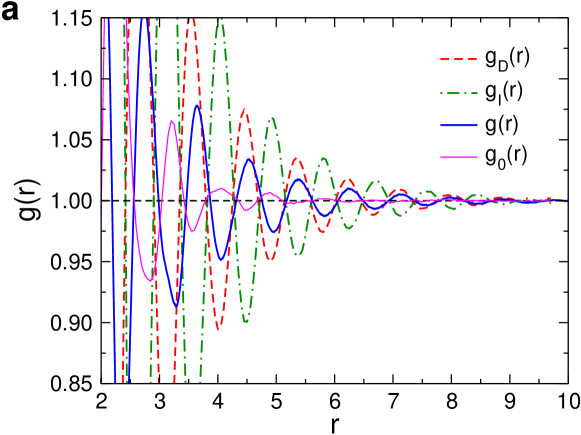The resulting distribution functions are shown in Extended Data Fig. 7. Panel a shows that, for intermediate and large distances, $g_{D}(r)$ has oscillations that are in phase with $g(r)$ whereas $g_{I}(r)$ has oscillations that are in anti-phase. The amplitudes of the oscillations in $g_{I}(r)$ and $g_{D}(r)$ are significantly larger than the ones found in $g(r)$, a result that is reasonable since the latter function is a weighted average of the two former ones and hence will be affected by cancellation effects. Furthermore we have done the same analysis also for the distribution function in the direction that corresponds to the mid-point of the line connecting two neighboring vertices of an icosahedron and a dodecahedron, defining thus $g_{0}(r)$. This correlation function is included in Extended Data Fig. 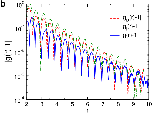7a as well and we see that it shows significantly smaller oscillations than $g(r)$, a result that is expected since one probes the structure in a direction which does not pass close to the locations that correspond to the vertices of the icosahedra/dodecahedra. Panel b shows that the length scale over which $g(r)$, $g_{I}(r)$, and $g_{D}(r)$ decay is basically independent of the function considered, demonstrating that they are indeed closely related to each other.

[30] S. Plimpton, Fast parallel algorithms for short-range molecular dynamics. J. Comp. Phys. 117, 1 (1995).

Extended Data Fig. 1: Radial distribution functions for several temperatures. The AA, AB, BB, and AN correlations are shown in panels a, b, c, and d, respectively. For the sake of clarity the different curves have been shifted vertically by multiples of 0.2.

Extended Data Fig. 2: Three dimensional distribution of the particles in the nearest neighbor shell. Density distribution $\rho(\theta,\phi,r)$ for $r=1.1$, i.e. the distance that corresponds to the particles in the first shell of the central particle. The temperature is $T=0.4$. a to c: Different perspectives of the density distribution on the sphere (see orientation of the coordinate system). A pronounced icosahedral-like symmetry can be recognized, see, e.g., the view of the distribution along the $x$-axis in panel a where the dashed lines indicate the connection between neighboring particles.

Extended Data Fig. 3: $l-$dependence of the angular power spectrum. a: $S_{\rho}(l,r)$ for $T=0.5$. The curves correspond to the indicated values of $r$. One sees that the signal for $l=6$, marked by a vertical dashed line, is pronounced at all distances. b: Comparison between the angular power spectra for $l=6$ and $l=7$. The $r-$dependence of $S_{\rho}(l,r)$ and $S_{\eta}(l,r)$ are qualitatively the same.

Extended Data Fig. 4: Angular power spectra and radial distribution function at short distances. $T=0.4$ and $l=6$. Note that the double peaks in the first shell, i.e. $r\approx 1.0$ originate from A-B (smaller peak) and A-A (bigger peak) correlations (see Fig. Extended Data Fig. 1).

Extended Data Fig. 5: Extracting length scales. a: $I(r,T)$, the integral of $S_{\eta}(r)$ for different temperatures. The length scale $\xi_{\eta}(T)$ is defined as the crossover point at which $I(r,T)$ starts to become a constant (see dashed lines). b: Local maxima of $S_{\rho}(6,r)$. c: Local maxima of $|g(r)-1|$. For both quantities, the data in the range $2.8<r<6.5$ are fitted with an exponential function to extract the corresponding length scale.

Extended Data Fig. 6: Structure factor and compressibility. a and b: Partial static structure factor $S(q)$ for the AA pairs for simulations at constant volume, a, and constant pressure, b. In panel b the pressure is equal to 8.0. The insets show $S(q)$ at small $q$. The two vertical dashed lines indicate the interval over which $S(q)$ was averaged in order to obtain the value $S_{0}(T)$ representing $S(q)$ at small $q$. c: $S_{0}(T)$ as obtained for the two ensembles as a function of inverse temperature. The magenta triangles are the compressibility from the NPT simulations. The solid lines are fits to the low-temperature data with a power-law. d: Same data as in panel c, now multiplied by $(1/T)^{\alpha}$, where the value of $\alpha$ is given in the legend. The horizontal dashed lines are guides to the eye to see better that the three data sets show at around $T=0.85$ a crossover in their $T-$dependence.

Extended Data Fig. 7: Anisotropic radial distribution function. Radial distribution function as measured in the direction of the vertices of the icosahedra, $g_{I}(r)$ and the direction of the vertices of the dodecahedra, $g_{D}(r)$. The function $g_{0}(r)$ probes the structure in the direction corresponding to the mid-point of the line connecting two neighboring vertices of an icosahedron and a dodecahedron. Panels a and b show these functions on a linear and log-scale, respectively. Also included is $g(r)$, i.e., the radial distribution function averaged over all directions.

Movie S1.
This movie shows the density distribution $\rho(\theta,\phi,r)$ as a function of the distance $r$ (left panel). The right panel shows the partial radial distribution function for A-N pairs (blue curve) as well as the normalized angular power spectrum $S_{\eta}(6,r)$ (red curve). The center of the vertical moving bar indicating the radius $r$ shown in the left panel. The temperature is $T=2.0$.

Movie S2.
This movie shows the density distribution $\rho(\theta,\phi,r)$ as a function of the distance $r$ (left panel). The right panel shows the partial radial distribution function for A-N pairs (blue curve) as well as the normalized angular power spectrum $S_{\eta}(6,r)$ (red curve). The center of the vertical moving bar indicating the radius $r$ shown in the left panel. The temperature is $T=0.4$.

References

- [1] K. Binder and W. Kob, Glassy Materials and Disordered Solids: An Introduction to Their Statistical Mechanics (World Scientific, Singapore, 2005).
- [2] D. J. Cosgrove, Growth of the plant cell wall, Nat. Rev. Mol. Cell Biol. 6, 850 (2005).
- [3] S. M. Becker and A. V. Kuznetsov, Transport in Biological Media (Academic Press, Amsterdam, 2013).
- [4] N. W. Ashcroft and N. D. Mermin, Solid State Physics (Holt-Saunders, New York, 1976).
- [5] J. P. Hansen and I. R. McDonald, Theory of Simple Liquids (Elsevier, Amsterdam, 1986).
- [6] P. S. Salmon, Decay of the pair correlations and small-angle scattering for binary liquids and glasses. J. Phys.: Condens. Matter. 18, 11443 (2006).
- [7] M. Leocmach and H. Tanaka, Roles of icosahedral and crystal-like order in the hard spheres glass transition. Nat. Comm. 3, 974 (2012).
- [8] C. P. Royall and S. R. Williams, The role of local structure in dynamical arrest. Phys. Rep. 560, 1 (2015).
- [9] S.S. Schoenholz, E.D. Cubuk, D.M. Sussman, E. Kaxiras, and A.J. Liu, A structural approach to relaxation in glassy liquids. Nat. Phys. 12, 469 (2016).
- [10] C. P. Royall and W. Kob, Locally favoured structures and dynamic length scales in a simple glass-former. J. Stat. Mech.: Theo. Exp. 2, 024001 (2017).
- [11] D. Coslovich and G. Pastore, Understanding fragility in supercooled Lennard-Jones mixtures. I. Locally preferred structures. J. Chem. Phys. 127, 124504 (2007).
- [12] A. J. Dunleavy, K. Wiesner, R. Yamamoto, and C. P. Royall, Mutual information reveals multiple structural relaxation mechanisms in a model glass former. Nat. Comm. 6, 6089 (2015).
- [13] H. Jonsson and H. C. Andersen, Icosahedral ordering in the Lennard-Jones liquid and glass. Phys. Rev. Lett. 60, 2295 (1988).
- [14] P. Wochner, C. Gutt, T. Autenrieth, T. Demmer, V. Bugaev, A. D. Ortiz, A. Duri, F. Zontone, G. Grübel, and H. Dosch, Proc. Natl. Acad. Sci. USA 106, 11511 (2009).
- [15] A. Malins, J. Eggers, C. P. Royall, S. R. Williams, and H. Tanaka, Identification of long-lived clusters and their link to slow dynamics in a model glass former. J. Chem. Phys. 138, 12A535 (2013).
- [16] Y. Q. Cheng and E. Ma, Atomic-level structure and structure-property relationship in metallic glasses. Prog. Mater. Sci. 56, 379 (2011).
- [17] D. B. Miracle, A structural model for metallic glasses. Nat. Mater. 3, 697 (2004).
- [18] C. Xia, J. Li, B. Kou, Y. Cao, Z. Li, X. Xiao, Y. Fu, T. Xiao, L. Hong, J. Zhang, W. Kob, and Y. Wang, Origin of non-cubic scaling law in disordered granular packing. Phys. Rev. Lett. 118, 238002 (2017).
- [19] G. Adam and J. H. Gibbs, On the temperature dependence of cooperative relaxation properties in glass-forming liquids. J. Chem. Phys. 43, 139 (1965).
- [20] X. Y. Xia and P. G. Wolynes, Fragilities of liquids predicted from the random first order transition theory of glasses. Proc. Natl. Acad. Sci. USA. 97, 2990 (2000).
- [21] D. Chandler and J. P. Garrahan, Dynamics on the way to forming glass: Bubbles in space-time. Annual Review of Physical Chemistry, 61, 191 (2010).
- [22] X. W. Fang, C. Z. Wang, Y. X. Yao, Z. J. Ding, and K. M. Ho, Atomistic cluster alignment method for local order mining in liquids and glasses. Phys. Rev. B 82, 184204 (2010).
- [23] X. W. Fang, C. Z. Wang, S. G. Hao, M. J. Kramer, Y. X. Yao, M. I. Mendelev, Z. J. Ding, R. E. Napolitano, and K. M. Ho, Spatially resolved distribution function and the medium-range order in metallic liquid and glass. Scient. Reps. 1, 194 (2011).
- [24] W. Kob and H. C. Andersen, Testing mode-coupling theory for a supercooled binary Lennard-Jones mixture I: The van Hove correlation function. Phys. Rev. E 51, 4626 (1995).
- [25] W. Götze, Complex dynamics of glass-forming liquids: A mode-coupling theory (Oxford University Press, Oxford, 2008).
- [26] W. K. Kegel and A. van Blaaderen, Direct Observation of Dynamical Heterogeneities in Colloidal Hard-Sphere Suspensions. Science 287, 290 (2000).
- [27] E. R. Weeks, J. C. Crocker, A. C. Levitt, A. Schofield, and D. A. Weitz, Three-dimensional direct imaging of structural relaxation near the colloidal glass transition. Science 287, 627 (2000).
- [28] J. F. Sherson, C. Weitenberg, M. Endres, M. Cheneau1, I. Bloch, and S. Kuhr, Single-atom-resolved fluorescence imaging of an atomic Mott insulator. Nature 467, 68 (2010).
- [29] B. Kou, Y. Cao, J. Li, C. Xia, Z. Li, H. Dong, A. Zhang, J. Zhang, W. Kob, and Y. Wang Granular materials flow like complex fluids. Nature 551, 360 (2017).
Acknowledgments
We thank D. Coslovich, G. Monaco, M. Ozawa, and K. Schweizer for discussions. Funding: Part of this work was supported by the China Scholarship Council grant 201606050112 and grant ANR-15-CE30-0003-02.
Author contributions: Z.Z. and W.K. designed the research and carried out the simulations. Z.Z. analyzed the data. Z.Z. and W.K. wrote the paper. Competing interests: The authors declare no competing financial interests. Data and materials availability: All data in the manuscript or the Materials are available from W. Kob upon reasonable request.
Methods
System and simulations.
The system we study is a
80:20 mixture of Lennard-Jones particles (type A and B) with
interactions given by , where
, , ,
, , , and
[24]. Here we use and
as the units of length and energy, respectively. We set
the mass of all particles equal to and the Boltzmann constant
is . Using the LAMMPS software 30 we simulate
a total of particles at constant volume (box size 43.68) and
temperature. At the lowest temperature, , the run was time steps (step size 0.005) for equilibration and the same length
for production, time spans that are sufficiently large to completely
equilibrate the system. For the analysis of the data we used 4 and 20
configuration for and , respectively.
Angular power spectrum. The coefficient for the expansion of the density distribution into spherical harmonics is given by
where is the complex conjugate of the spherical harmonic
function of degree and order . In practice this integration was
done by sampling the integrand over up to points for each
shell of width 0.4.
Radial distribution functions.
In Extended Data Fig. 1 we show
the three partial radial distribution functions as well as the
correlation function between an A particle and any other particle (AN).
The curves correspond to different temperatures (see legend). These graphs show
that the dependence of is very smooth, as expected for a
system that is a good glass-former.