Effective approximation of heat flow evolution of the Riemann function, and a new upper bound for the de Bruijn-Newman constant
Abstract.
For each , define the entire function
where is the super-exponentially decaying function
This is essentially the heat flow evolution of the Riemann function. From the work of de Bruijn and Newman, there exists a finite constant (the de Bruijn-Newman constant) such that the zeroes of are all real precisely when . The Riemann hypothesis is equivalent to the assertion ; recently, Rodgers and Tao established the matching lower bound . Ki, Kim and Lee established the upper bound .
In this paper we establish several effective estimates on for , including some that are accurate for small or medium values of . By combining these estimates with numerical computations, we are able to obtain a new upper bound unconditionally, as well as improvements conditional on further numerical verification of the Riemann hypothesis. We also obtain some new estimates controlling the asymptotic behavior of zeroes of as .
1. Introduction
Let denote the function
| (1) |
where denotes the Riemann function
| (2) |
(which is an entire function after removing all singularities) and is the Riemann function. Then is an entire even function with functional equation , and the Riemann hypothesis (RH) is equivalent to the assertion that all the zeroes of are real.
It is a classical fact (see [27, p. 255]) that has the Fourier representation
where is the super-exponentially decaying function
| (3) |
The sum defining converges absolutely for negative also. From Poisson summation one can verify that satisfies the functional equation (i.e., is even); this fact is of course closely related to the functional equation for .
De Bruijn [5] introduced (with somewhat different notation) the more general family of functions for , defined by the formula
| (4) |
As noted in [9, p.114], one can view as the evolution of under the backwards heat equation . As with , each of the are entire even functions with functional equation ; from the super-exponential decay of we see that the are in fact entire of order . It follows from the work of Pólya [19] that if has purely real zeroes for some , then has purely real zeroes for all ; de Bruijn showed that the zeroes of are purely real for . Newman [14] strengthened this result by showing that there is an absolute constant , now known as the De Bruijn-Newman constant, with the property that has purely real zeroes if and only if . The Riemann hypothesis is then clearly equivalent to the upper bound . Recently in [22] the complementary bound was established, answering a conjecture of Newman [14], and improving upon several previous lower bounds for [6, 15, 8, 7, 16, 23]. Furthermore, Ki, Kim, and Lee [10] sharpened the upper bound of de Bruijn [5] slightly to .
In this paper we improve the upper bound:
Theorem 1.1 (New upper bound).
We have .
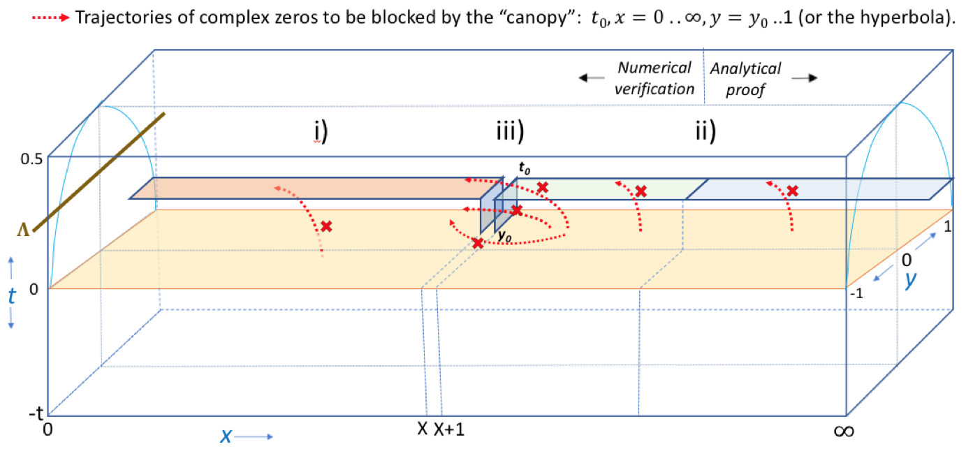
The proof of Theorem 1.1 combines numerical verification with some new asymptotics and observations about the which may be of independent interest. Firstly, by analyzing the dynamics of the zeroes of , we establish in Section 3 the following criterion for obtaining upper bounds on :
Theorem 1.2 (Upper bound criterion).
Suppose that and obey the following hypotheses:
-
(i)
(Numerical verification of RH at initial time ) There are no zeroes with and .
-
(ii)
(Asymptotic zero-free region at final time ) There are no zeroes with and .
-
(iii)
(Barrier at intermediate times) There are no zeroes with , , and .
Then .
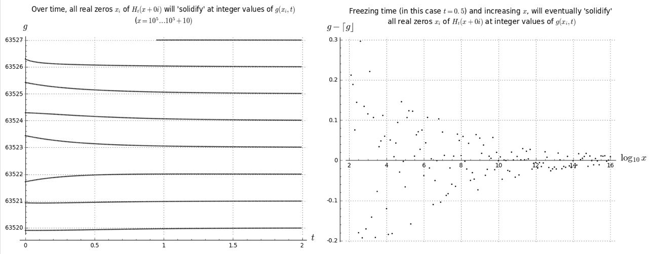
Informally, hypothesis (i) implies that at time , there are no zeroes with large values of to the left of the barrier region in (iii). The absence of zeroes in that barrier, together with a continuity argument and an analysis of the time derivative of each zero, can then be used to show that for later times , there continue to be no zeroes with large values of to the left of the barrier; see Figure 1. Hypothesis (ii) then gives the complementary assertion to the right of the barrier, and one can use an existing theorem of de Bruijn (Theorem 3.2) to conclude.
In practice, we have found it convenient numerically to replace the barrier region in Theorem 1.2 with the larger and simpler region
We will obtain Theorem 1.1 by applying Theorem 1.2 with the specific numerical choices , , and . The reason we choose close to is that this is near the limit of known numerical verifications of the Riemann hypothesis such as [18], which we need for the hypothesis (i) of the above theorem; the shift is in place to make the partial Euler product large, which helps in keeping the functions large in magnitude, which in turn is helpful for numerical verifications of (ii) and (iii); see also Figure 11. The choices are then close to the limit of our ability to numerically verify hypothesis (ii) for this choice of . (The hypothesis (iii) is also verified numerically, but can be done quite quickly compared to (ii), and so does not present the main bottleneck to further improvements to Theorem 1.1.) Further upper bounds to can be obtained if one assumes the Riemann hypothesis to hold up to larger heights than that in [18]: see Section 10.
To verify (ii) and (iii), we need efficient approximations (of Riemann-Siegel type) for in the regime where are bounded and is large. For sake of numerically explicit constants, we will focus attention on the region
| (5) |
though the results here would also hold (with different explicit constants) if the numerical quantities were replaced by other quantities.
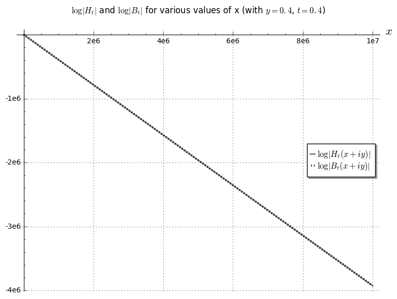
A key difficulty here is that decays exponentially fast in (basically because of the Gamma factor in (2)); see Figure 3. This means that any direct attempt to numerically establish a zero-free region for for large would require enormous amounts of numerical precision. To get around this, we will first renormalise the function by dividing it by a nowhere vanishing explicit function (basically a variant of the aforementioned Gamma factor) that removes this decay. To describe this function, we first introduce the function defined by the formula
| (6) |
where denotes the standard branch of the complex logarithm, with branch cut at the negative axis and imaginary part in . One may interpret as the Stirling approximation to the factor appearing in (1), (2); it decays exponentially as one moves to infinity along the critical strip. We may form a holomorphic branch of the logarithm of by the formula
| (7) |
differentiating this, we see that the logarithmic derivative of this function, defined by
| (8) |
is given explicitly by the formula
| (9) |
For any time , we then define the deformation of by the formula
| (10) |
for any . In the region (5), we introduce the quantity
| (11) |
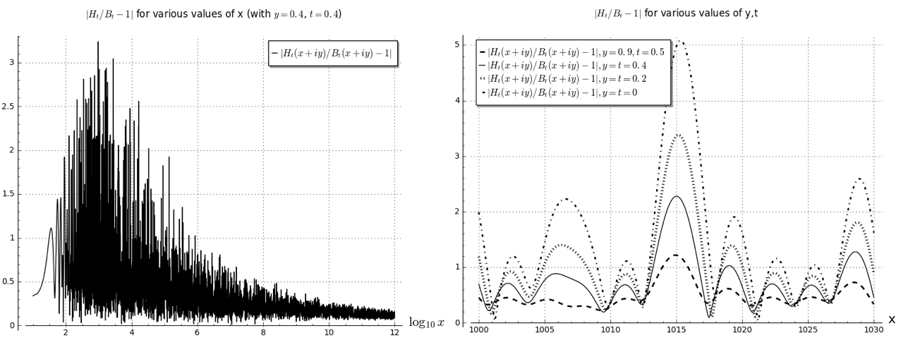
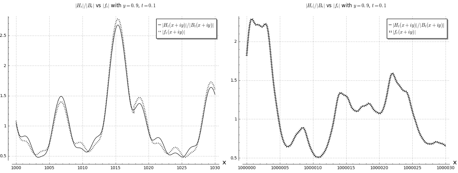
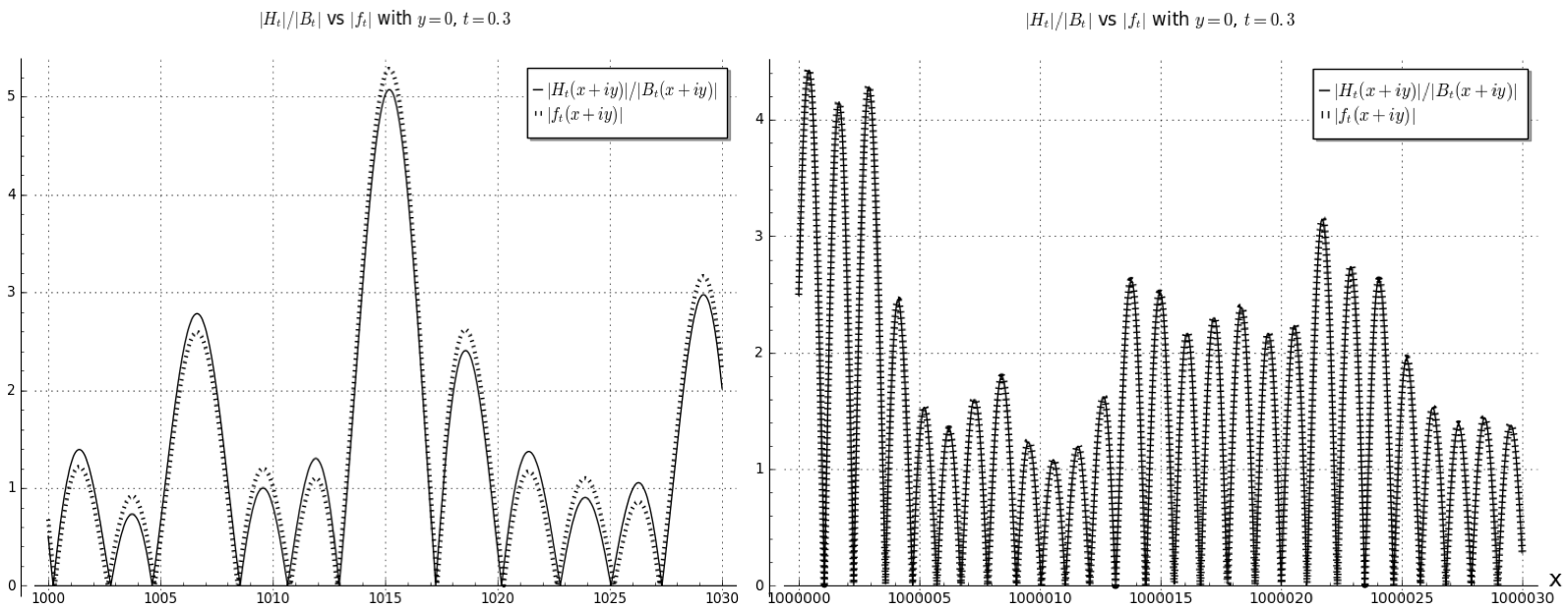
For fixed and , is non-vanishing, and it is easy to verify the asymptotic . As it turns out, is an asymptotic approximation to in the region (5), in the sense that
| (12) |
for any fixed and ; see Figure 2. (However, the convergence of (12) is not uniform as approaches zero.)
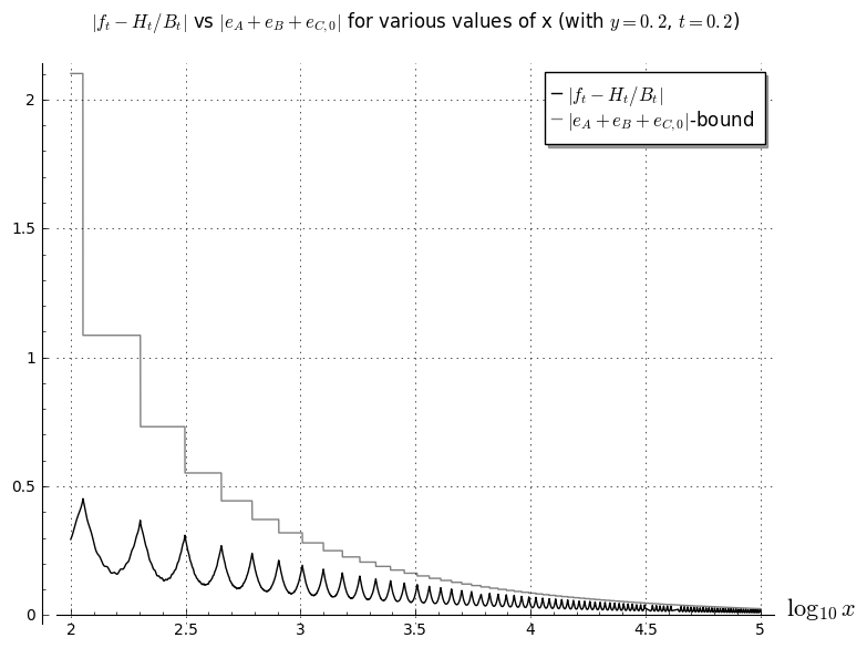
In fact we have the following significantly more accurate approximation (of Riemann-Siegel type) with effective error estimates. For any real number , let denote a quantity that is bounded in magnitude by . We also use to denote the positive part of a real number .
Theorem 1.3 (Effective Riemann-Siegel approximation to ).
This theorem will be proven in Section 6; see Figures 4, 5 for a numerical illustration of the approximation. The strategy is to express as a convolution of with a gaussian heat kernel, then apply an effective Riemann-Siegel expansion to to rewrite as the sum of various contour integrals; see Section 4 for details. One then uses the saddle point method to shift each such contour to a location that is suitable for effective estimation. We remark that is a holomorphic function of in the region (5) as long as is constant, but has jump discontinuities when is incremented.
From (13) and the triangle inequality, we have a numerically verifiable criterion to establish non-vanishing of at a given point:
Corollary 1.4 (Criterion for non-vanishing).
Actually, for some regions of we will use a more complicated criterion than (25), in order to exploit the argument principle. To numerically estimate in a feasible amount of time, we will use Taylor expansion to be able to efficiently compute many values of simultaneously (see Section 7), and for some ranges of the parameters we will also use an Euler product mollifier to reduce the amount of oscillation in the sum (see Section 8.5).
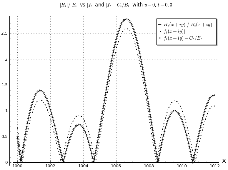
For fixed and sufficiently large, we have the asymptotics
for some absolute constant ; see Proposition 9.1(i) and its proof. This gives the crude asymptotic (12) in the region (5) at least. In practice, the term numerically dominates the term, although both errors will be quite small in the ranges of under consideration; in particular, for the ranges needed to verify conditions (ii) and (iii) of Theorem 1.2, we can make and both significantly smaller than . In the spirit of expanding the Riemann-Siegel approximation to higher order, we also obtain an even more accurate explicit approximation in which a correction term is added to , and the error term is replaced by a smaller quantity ; see (69) and Figure 8.
In addition to establishing upper bounds such as Theorem 1.1, one can use Theorem 1.3 and Corollary 1.4 (together with variants in slightly larger regions than (5), for instance if is allowed to be as large as ) to obtain asymptotic control on the zeroes of , refining previous work of Ki, Kim, and Lee [10]. Indeed, in Section 9 we will establish
Theorem 1.5 (Distribution of zeroes of ).
Let , let be a sufficiently large absolute constant, and let be a sufficiently small absolute constant. For , define
and for all , let be the unique real number greater than such that
| (26) |
(This is well-defined since the is increasing in for .)
-
(i)
If and , then , and
for some .
-
(ii)
Conversely, for each there is exactly one zero in the disk (and by part (i), this zero will be real and lie within of ).
-
(iii)
If , the number of zeroes with real part between and (counting multiplicity) is
-
(iv)
For any , one has
and
Here and in the sequel we use to denote the estimate for some constant that is absolute (in particular, is independent of and ).
Roughly speaking, these estimates tell us that the zeroes of behave (on macroscopic scales) like those of in the region , and are very evenly spaced (and on the real axis) outside of this range. The factor in (26) indicates that as time advances, the zeroes (or at least those with large values of ) will tend to move towards the origin at a speed of approximately . Although we will not prove this here, the conclusions (i) and (iii) suggest that one in fact has an asymptotic of the form
when ; in particular (since the sawtooth function has average value ) one would have the heuristic approximation
after performing some averaging in , thus recovering the familiar term in the usual averaged asymptotics for .
The results in Theorem 1.5 refine previous results of Ki, Kim, and Lee [10, Theorems 1.3, 1.4], which gave similar results but with constants that depended on in a non-uniform (and ineffective) fashion, and error terms that were of shape rather than in the limit (holding fixed). The results may also be compared with those in [3], who (in our notation) show that assuming RH, the zeroes of are precisely the solutions to the equation
for integer , where is the phase of and one chooses a branch of the argument so that the left-hand side is when .
Remark 1.6.
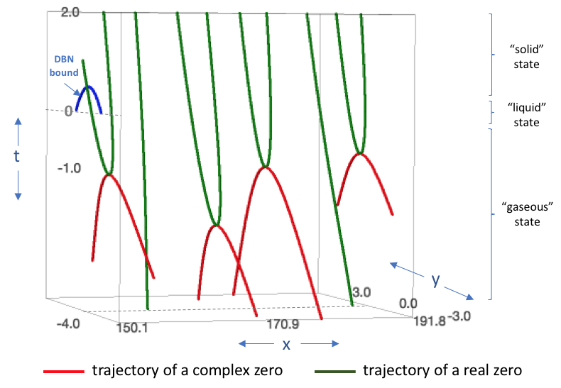
One can draw an analogy between the various potential behaviours of zeroes of and the three classical states of matter. A “gaseous” state corresponds to the situation in which some fraction of the zeroes of are strictly complex. A “liquid” state corresponds to a situation in which the zeroes are real, but disordered (with highly unequal spacings between zeroes). A “solid” state corresponds to a situation in which the zeroes are real and arranged roughly in an arithmetic progression. Thus for instance the Riemann hypothesis and the GUE hypothesis assert (roughly speaking) that the zeroes of should exhibit liquid behaviour everywhere, while Theorem 1.5 asserts that the zeroes of , “solidify” in the region . Below this region we expect liquid behaviour. In general, as the parameter increases, the zeroes appear222This is the picture for positive at least. As becomes very negative, it appears that the “gaseous” zeroes become more ordered again, for instance organizing themselves into curves in the complex plane. See [21] for further discussion of this phenomenon. to “cool” down, transitioning from gaseous to liquid to solid type states; see [22] for some formalisations of this intuition.
1.1. About this project
This paper is part of the Polymath project, which was launched by Timothy Gowers in February 2009 as an experiment to see if research mathematics could be conducted by a massive online collaboration. The current project (which was administered by Terence Tao) is the fifteenth project in this series. Further information on the Polymath project can be found on the web site michaelnielsen.org/polymath1. Information about this specific project may be found at
michaelnielsen.org/polymath1/index.php?title=De_Bruijn-Newman_constant
and a full list of participants and their grant acknowledgments may be found at
michaelnielsen.org/polymath1/index.php?title=Polymath15_grant_acknowledgments
We thank the anonymous referees for their careful reading of the paper and for several useful corrections and suggestions.
2. Notation
We use the standard branch of the logarithm to define the standard complex powers , and in particular define the standard square root . We record the familiar gaussian identity
| (27) |
for any complex numbers with .
When using order of magnitude notation such as , any expression of the form using this notation should be interpreted as the assertion that any quantity of the form is also of the form , thus for instance . (In particular, the equality relation is no longer symmetric with this notation.)
If is a meromorphic function, we use to denote its derivative. We also use to denote the reflection of . Observe from analytic continuation that if is holomorphic on a connected open domain containing an interval in , and is real-valued on , then it is equal to its own reflection: (since the holomorphic function has an uncountable number of zeroes).
3. Dynamics of zeroes
In this section we control the dynamics of the zeroes of in order to establish Theorem 1.2. As is even with functional equation , the zeroes are symmetric around the origin and the real axis; from (4) and the positivity of , we also see that for all , so there are no zeroes on the imaginary axis. From the super-exponential decay of and (4) we see that the entire function is of order ; by Jensen’s formula, this implies that the number of zeroes in a large disk is at most as .
We begin with the analysis of the dynamics of a single zero of :
Proposition 3.1 (Dynamics of a single zero).
Let , and let be an enumeration of the zeroes of in (counting multiplicity), with the symmetry condition .
-
(i)
If is such that is a simple zero of , then there exists a neighbourhood of , a neighbourhood of in , and a smooth map such that for every , is the unique zero of in . Furthermore one has the equation
(28) where the sum is over those with , and the prime means that the and terms are summed together (except for the term, which is summed separately) in order to make the sum convergent.
-
(ii)
If is such that is a repeated zero of of order , then there is a neighbourhood of such that for sufficiently close to , there are precisely zeroes of in , and they take the form
for as , where are the roots of the Hermite polynomial
(29) (30) and the implied constant in the notation can depend on , , and .
The differential equation (28) was previously derived in [9, Lemma 2.4] in the case (in which all zeroes are real and simple); however, in our applications we also need to consider the regime in which the zeroes are permitted to be complex or repeated. The roots appearing in Proposition 3.1(ii) can be given explicitly for small values of as
when ,
when , and
when . From (29) and iterating Rolle’s theorem we see that all the roots of are real; from the Hermite equation and the Picard uniqueness theorem for ODE we see that the zeroes are all simple.
Proof.
First suppose we are in the situation of (i). As is simple, is non-zero at ; since is a smooth function of both and , we conclude from the implicit function theorem that there is a unique solution to the equation
with in a sufficiently small neighbourhood of , if is in a sufficiently small neighbourhood of ; furthermore, depends smoothly on , and agrees with when . Differentiating the above equation at , we obtain
where the primes denote differentiation in the variable. On the other hand, from (4) and differentiation under the integral sign (which can be justified using the rapid decrease of ) we have the backwards heat equation
| (31) |
for all . Inserting this into the previous equation, we conclude that
| (32) |
noting that the denominator is non-vanishing by the hypothesis that the zero at is simple. Henceforth we omit the dependence on for brevity. From Taylor expansion of , , and around the simple zero we see that
| (33) |
On the other hand, as is even, non-zero at the origin (as follows from (4) and the positivity of ), and entire of order , we see from the Hadamard factorization theorem that
where the prime indicates that the and factors are multiplied together. The product is locally uniformly convergent, so we may take logarithmic derivatives and conclude that
Inserting this into (32), (33) and using the continuity of at (which follows from the growth in the number of zeroes, either from the dominated convergence theorem or the Weierstrass -test), we obtain the claim (i).
Now we prove (ii). We abbreviate as . By Taylor expansion we have
as for any fixed integer and some non-zero complex number (with the implied constant in the notation allowed to depend on , , ); applying the backwards heat equation (31) we thus have
Performing Taylor expansion in time and using (30), we conclude that in the regime , one has the bound
as , using (say) the standard branch of the square root. By the inverse function theorem (and the simple nature of the zeroes of ), we conclude that for sufficiently close but not equal to , we have zeroes of of the form
By Rouche’s theorem, if is a sufficiently small neighborhood of then these are the only zeroes of in for sufficiently close to . The claim follows. ∎
Next, we recall the following bound of de Bruijn:
Theorem 3.2.
Suppose that and is such that there are no zeroes with and . Then for any , there are no zeroes with and . In particular one has .
Proof.
See [5, Theorem 13]. ∎
We are now ready to prove Theorem 1.2. The main step is to establish
Proposition 3.3 (Zero-free region criterion).
Suppose that and obey the following hypotheses:
-
(i)
There are no zeroes with and .
-
(ii)
There are no zeroes with and .
-
(iii)
There are no zeroes with , , and .
Then there are no zeroes with and .
Proof.
It is well known that the Riemann function has no zeroes outside of the strip , hence there are no zeroes with . By Theorem 3.2, we may thus remove the upper bound constraints , , and from (i), (ii), and (iii) respectively.
By hypotheses (ii), (iii) and the symmetry properties of , it suffices to show that for every , there are no zeroes with and , where . By hypothesis (i), this is true at time . Suppose the claim failed for some time . Let be the minimal time in which this occurred (such a time exists because varies continuously in , and there are no zeroes with (say) ). From Rouche’s theorem (or Proposition 3.1) we conclude that there is a zero with on the boundary of the region . The right side of this boundary is ruled out by hypothesis (iii), and (as mentioned at the start of the section) the left side is ruled out by (4) and the positivity of . Thus by the symmetry properties of we must have
for some .
Suppose first that has a repeated zero at . Using Proposition 3.1(ii) and observing (from the symmetry of ) that at least one of the roots is positive, we then see that for sufficiently close to , has a zero in the region , contradicting the minimality of . Thus the zero of must be simple. In particular, by Proposition 3.1(i) we can write for some smooth function in a neighbourhood of obeying (28), such that is a zero of for all close to . We will prove that
| (34) |
which implies that there is a zero of in the region for sufficiently close to , giving the required contradiction.
The right-hand side of (34) is
By Proposition 3.1(i), the left-hand side of (34) is
where we write . Clearly any zero with imaginary part in gives a non-positive contribution to this sum, the contribution of the zero is , the contribution of the zero vanishes, and the contribution of is negative. Grouping the remaining zeroes with their complex conjugates, it then suffices to show that
whenever . Cross-multiplying and canceling like terms, this inequality eventually simplifies to
But from the hypothesis (iii) and the assumption , we have , so . On the other hand from Theorem 3.2 one has , giving the required contradiction. ∎
4. Applying the fundamental solution for the heat equation
As discussed in the introduction, we will establish Theorem 1.3 by writing in terms of using the fundamental solution to the heat equation. Namely, for any , we have from (27) that
for any complex and either choice of sign . Multiplying by and averaging, we conclude that
for any complex . Multiplying by and using Fubini’s theorem, we conclude the heat kernel representation
for any complex . Using (1), we thus have
| (35) |
Remark 4.1.
We have found numerically that the formula (35) gives a fast and accurate means to compute when is of moderate size, e.g., if with and . However, we will not need to directly compute the right-hand side of (35) for our application to bounding , as we will only need to control for large values of , and we will shortly develop tractable approximations of Riemann-Siegel type that are more suitable for this regime.
We now combine this formula with expansions of the Riemann -function. From [27, (2.10.6)] we have the Riemann-Siegel formula
| (36) |
for any complex that is not an integer (in order to avoid the poles of the Gamma function), where is the contour integral
with any infinite line oriented in the direction that crosses the interval . From the residue theorem (and the gaussian decrease of along the and directions) we may expand
for any non-negative integer , where are the meromorphic functions
| (37) | ||||
| (38) |
and denotes any infinite line oriented in the direction that crosses the interval . For any that is not purely imaginary, we see from Stirling’s approximation that the functions and grow slower than gaussian as (indeed they grow like , where the implied constants depend on ). From this and (35), (36) we conclude that
| (39) |
for any , any that is not purely imaginary, and any non-negative integer , where are defined for non-real by the formulae
these can be thought of as the evolutions of respectively under the forward heat equation.
The functions grow slower than gaussian as long as the imaginary part of is bounded and bounded away from zero. As a consequence, we may shift contours (replacing by ) and write
| (40) |
for any complex number with having the same sign. Similarly we may write
| (41) |
for any complex number with having the same sign. In the spirit of the saddle point method, we will select the parameters later in the paper in order to make the integrands in (40), (41) close to stationary in phase at , in order to obtain good estimates and approximations for these terms.
5. Elementary estimates
In order to explicitly estimate various error terms arising in the proof of Theorem 1.3, we will need the following elementary estimates:
Lemma 5.1 (Elementary estimates).
Let .
-
(i)
If and are such that , then
More generally, if and are such that , then
-
(ii)
If , then
or equivalently
-
(iii)
If , then
-
(iv)
We have
-
(v)
If is a complex number with or , then
-
(vi)
If and and , then
Proof.
Claim (i) follows from the geometric series formula
whenever .
For Claim (ii), we use the Taylor expansion of the logarithm to note that
which on comparison with the geometric series formula
gives the claim. Similarly for Claim (iii), we may compare the Taylor expansion
with the geometric series formula
and note that for all .
Claim (iv) follows from the trivial identity and the elementary inequality . For Claim (v), we may use the functional equation to assume that . From the work of Boyd [4, (1.13), (3.1), (3.14), (3.15)] we have the effective Stirling approximation
where the remainder obeys the bound
for and
for , where is the constant
In the latter case, we have by hypothesis, and hence . We conclude that in all ranges of of interest, we have
and hence by Claim (i)
and the claim then follows by Claim (ii).
For Claim (vi), it suffices to show that the function is non-increasing for . Since and the second factor is monotone decreasing in , it suffices to show that is non-increasing in this region. Taking logarithms and differentiating, we wish to show that . But this is clear since and . ∎
6. Proof of Theorem 1.3
In this section we establish Theorem 1.3. The strategy is to use the expansion (39), which turns out to be an effective approximation in the region (5), since we will be able to ensure that quantities such as or , with , stay away from the real axis where the poles of are located (and also where the error terms in the Riemann-Siegel approximation deteriorate).
Accordingly, we will need effective estimates on the functions appearing in Section 4. We will treat these two functions separately.
6.1. Estimation of
We recall the function defined in (8). From differentiating (9) we see that
| (42) |
whenever . If , we conclude in particular the useful bound
| (43) |
thanks to Lemma 5.1(i).
We also recall the function and the coefficients from (10), (15) respectively. It turns out we have a good approximation
More precisely, we have
Proposition 6.1 (Estimate for ).
Let be real, let , let be a positive integer, and let . Then
where
| (44) |
Proof.
From (37), (6) and Lemma 5.1(v) one has
whenever . Let denote the quantity
| (45) |
this is the logarithmic derivative of at . By (9) and the hypothesis , the imaginary part of may be lower bounded by
| (46) |
in particular, and have imaginary parts of the same sign. We can now apply (40) to obtain
From (46) we see that has imaginary part at least . Thus
From (43) we have
for all on the line segment between and . Applying Taylor’s theorem with remainder to the branch of the logarithm defined in (7), we conclude that
Combining these estimates, writing , estimating by , and simplifying, we conclude that
Using (45), (10), (15) we see that
and so it suffices to show that
Since integrates to one, it suffices by Lemma 5.1(iv) to show that
Since , we can remove the terms from both sides and reduce to showing that
| (47) |
Using (27), the left-hand side may be calculated exactly as
Applying Lemma 5.1(ii) and using the hypotheses , , one has
and the claim follows. ∎
6.2. Estimation of
Proposition 6.2.
Let be real and , and define the quantities
| (48) | ||||
| (49) | ||||
| (50) | ||||
| (51) | ||||
| (52) |
Let be a positive integer. Then we have the expansion
where is independent of and is given explicitly by the formula
| (53) |
(removing the singularities at ), while for the are complex numbers obeying the bounds
| (54) |
for and
| (55) |
for , while the error term is a complex number obeying the bounds
| (56) |
for , and
| (57) |
if and .
Proof.
Note that ranges in the interval . One can show that
| (58) |
for all ; this follows for instance from the case of [2, Theorem 6.1]. See also Figure 10.
Informally, the above proposition (and (38), (6)) yield the approximation
If one writes , then by using the approximation for the log-derivative of , one can then obtain the approximate formula
In fact we have the more general approximation
where . More precisely, we have
Proposition 6.3 (Estimate for ).
Proof.
We apply (41) with to obtain
From (38) we have
for any positive integer that we permit to depend (in a measurable fashion) on , where . From (6) and Lemma 5.1(v) we thus have
From (43) and Taylor expansion of the logarithm defined in (7), we have
and hence (bounding by )
We conclude (bounding ) that
Bounding , we have
Putting all this together, we obtain
We separate the term from the rest. By Lemma 5.1(iv) and the fact that integrates to one, we can write the above expression as
| (60) |
where
and
Bounding and using (27) we obtain
Applying Lemma 5.1(ii) and using the hypotheses , , one has
and hence
With and , one has . By the mean value theorem we then have
| (61) |
Now we work on . Making the change of variables , we have
where is a positive integer parameter that can depend arbitrarily on (as long as it is measurable, of course).
We choose to equal when and when , so that Proposition 6.2 applies. The expression
is then bounded by
| (62) |
for and
| (63) |
for . One can calculate that
and
and hence we can bound (63) by
For , we can estimate (62) by
thanks to Lemma 5.1(i). For , we observe that if then
and hence by the geometric series formula
and similarly
and hence we can bound (63) by
By Lemma 5.1(i) we have
and thus we can bound (63) by
Putting this together, we conclude that
for all (positive or negative). We conclude that , where
| (64) |
For , we translate by to obtain
and hence by (27)
| (65) |
One can write
| (66) |
while by Lemma 5.1(ii) we have
| (67) |
We conclude that
From Lemma 5.1(i) and the hypothesis , we have
and therefore by a further application of Lemma 5.1(i)
and thus
With and one has
and hence
and
Now we turn to , which will end up being extremely small compared to or . By (64) and the Fubini-Tonelli theorem, we have
Since , , and , we have and ; since , we may thus lower bound by . Since , we can upper bound by (say) , thus
We can bound , in the range of integration and thus
bounding
we conclude that
For one can easily verify that ; discarding the and factors we thus have
(say). Since
we thus have
Inserting this and (61), (58) into (60), and crudely bounding by , we obtain the claim. ∎
6.3. Combining the estimates
Combining Propositions 6.1, 6.3 with (39) and the triangle inequality (and noting that , and , and that has magnitude ), we conclude the following “ approximation to ”:
Corollary 6.4 ( approximation).
In our applications, we will just use the cruder “” approximation that is immediate from the above corollary and (58):
Corollary 6.5 ( approximation).
We can now prove Theorem 1.3. Dividing by the expression from (11), and using (14), we conclude that
| (69) |
and
| (70) |
where
| (71) | ||||
| (72) | ||||
| (73) | ||||
| (74) |
and where were defined in (16), (17), (18). Note also from (68), (49), (50) that is given by (19).
To conclude the proof of Theorem 1.3 it thus suffices to obtain the following estimates.
Proposition 6.6 (Estimates).
Let the notation and hypotheses be as above.
-
(i)
One has
-
(ii)
One has
-
(iii)
One has
-
(iv)
One has
-
(v)
One has
-
(vi)
One has
and
Note that to obtain the bound (24) from Proposition 6.6(vi) we may simply use the inequality for any , and then bound .
Proof.
From the mean value theorem (and noting that , so that ), we have
for some . From (8), (10) we have
From (43) one has
| (75) |
and from Taylor expansion we also have
from (9) one has
and hence
| (76) |
Inserting these bounds, we conclude that
Expanding this out, we have
In the region (5), which implies that , we have
and thus
The function is decreasing for thanks to Lemma 5.1(vi), hence
Claim (i) follows. We remark that one can improve the factor here by Taylor expanding to second order rather than first order, but we will not need to do so here.
To prove claim (ii), it suffices by (21) to show that
By (9) one has
We bound and calculate
Lower bounding the numerator by its nonnegative part and then lower bounding by , we obtain the claim.
Claim (iii) is immediate from (75) and the fundamental theorem of calculus. Now we turn to (iv), (v). From (76) one has
for either choice of sign . In particular, we have
| (77) |
For any , we have
in the region (5), the right-hand side is certainly bounded by , so that
and hence
In the region (5) we have , we see from Lemma 5.1(vi) (after squaring) that is decreasing in . Thus
Similarly, in (5) we also have
We conclude from (44) that
Inserting this bound into (71), (72), we obtain claims (iv), (v).
Now we establish (vi). From (10) we have
Note that . From (43) we see that for any on the line segment between and . From Taylor’s theorem with remainder applied to a branch of , and noting that , we conclude that
For and we have
and from (9) one has
and hence
Bounding and , this becomes
and hence
By repeating the proof of (77) we have
As before, in the region (5) we have
and thus
thanks to Lemma 5.1(i). Finally, since in (5), one has
and hence by (59)
Hence
giving the claim (substituting and ). ∎
7. Fast evaluation of multiple sums
Fix . For the verification of the barrier criterion (Theorem 1.2(iii)) using Corollary 1.4, we will need to evaluate the quantity to reasonable accuracy for a large number of values of in the vicinity of a fixed complex number . From (14) we have
| (78) |
where is given by (15), is given by (16), is given by (19) and
and
with defined by (17), (18). In practice the exponents will be rather small, and will be fixed (in our main verification we will in fact have ).
A naive computation of for values of would take time , which turns out to be somewhat impractical for for the ranges of we will need; indeed, for our main theorem, the total number of pairs at which we need to perform the evaluation is (spread out over values of ), and direct computation of all this data required hours of computer time, which was still feasible at this order of magnitude of but would not scale to significantly higher magnitudes. However, one can significantly speed up the computation (to about hours) to extremely high accuracy by using Taylor series expansion to factorise the sums in (78) into combinations of sums that do not depend on and thus can be computed in advance.
We turn to the details. To make the Taylor series converge333One can obtain even faster speedups here by splitting the summation range into shorter intervals and using a Taylor expansion for each interval, although ultimately we did not need to exploit this. faster, we recenter the sum in , writing
for any function , where . We thus have
where
and
We discuss the fast computation of for multiple values of ; the discussion for is analogous. We can write the numerator as
writing , this becomes
By Taylor expanding444It is also possible to proceed by just performing Taylor expansion on the second exponential and leaving the first exponential untouched; this turns out to lead to a comparable numerical run time. the exponentials, we can write this as
and thus the expression can be written as
where
If we truncate the summations at some cutoff , we obtain the approximation
The quantities may be evaluated in time , and then the sums for values of may be evaluated in time , leading to a total computation time of which can be significantly faster than even for relatively large values of . We took , which is more than adequate to obtain extremely high accuracy555One can obtain more than adequate analytic bounds for the error (which are several orders of magnitude more than necessary) for the parameter ranges of interest by very crude bounds, e.g., bounding and by (say) , and relying primarily on the and terms in the denominator to make the tail terms small. We omit the details as they are somewhat tedious.; for ; see Figure 13. The code for implementing this may be found in the file
dbn_upper_bound/pari/barrier_multieval_t_agnostic.txt
in the github repository [20].
8. A new upper bound for the de Bruijn-Newman constant
In this section we prove Theorem 1.1.
8.1. Selection of parameters
As stated in the introduction, it suffices to verify the conditions (i), (ii), (iii) of Theorem 1.2 , , and , where .
The choice is due to the limitations of our numerical verifications, particularly the known numerical verification of RH. We now explain the choice of . Recall the familiar Euler product factorization
for the Riemann zeta function. This leads to the heuristic
for some small prime cutoff , where and we are extremely vague as to what the proportionality symbol means. This heuristic extends to non-zero times as
and we also have
| (79) |
One can non-rigorously justify the latter assertion by by inspecting the first series of in (14) and ignoring the fact that the sequence is not multiplicative when .
We will be relying heavily on Corollary 1.4, and therefore seek to ensure that is as large as possible. It would therefore seem to be advantageous to try to work as much as possible in regions where Euler product
is small, which heuristically corresponds to being close to an integer for (so that has argument close to zero). If one chooses to lie in the vicinity of
then indeed the fractional parts for are somewhat close to zero:
We found this shift by the following somewhat ad hoc procedure. We first introduced the quantity
which is the exponent corresponding to (where the minimum value of in the barrier region is expected to occur). We numerically located candidate integers for which the quantity
exceeded a threshold (we chose ), to obtain seven candidates for : , , , , , , and . Among these candidates, we selected the value of which maximised the quantity
namely (this quantity being for this value of ).
8.2. Verifications of claims
Claim (i) of Theorem 1.2 is immediate from the result of Platt [18] that all the non-trivial zeroes of with imaginary part between and lie on the critical line . For the remaining claims (ii), (iii) of Theorem 1.2, it will suffice to verify that for the following three regions of :
-
(ii)
, , and .
-
(iii)
, , and .
Here we have enlarged the region (iii) for simplicity. Both of these regions lie in (5). We can of course replace by .
Set
so in particular
| (80) |
where
Write and . In region (ii) we then have , while in region (iii) we have . It will now suffice to verify in the following three regions:
-
(a)
When , , , and .
-
(b)
When , , , and .
-
(c)
When , , and .
In all three regions we use the following approximation:
Proposition 8.1.
Proof.
By Theorem 1.3 it suffices to show that
From Theorem 1.3 again, we have
| (82) |
where
| (83) |
and
| (84) |
From Lemma 5.1(vi), the quantity is monotone decreasing in in the region (5). Thus we have
| (85) |
whenever and . Computing the right-hand side, we conclude that
and hence by Taylor expansion
(say). Also, from Theorem 1.3 and (83) we can bound
For , , and we see from Lemma 5.1(vi) that
and
and thus
| (86) |
Thus
To estimate , we use Proposition 6.6(ii) or (22), together with the inequality
to obtain
(say). Since is non-increasing in , we conclude
Since
, and , it is easy to see that
and hence by (15)
for all . Therefore
and hence by the integral test
so that (by (84))
We have
(say), and hence
From Lemma 5.1(vi), the right-hand side is monotone decreasing in the region , thus
Meanwhile, from Proposition 6.6(vi) one has
From Lemma 5.1(vi), the quantity is monotone decreasing in in (5), hence is also monotone decreasing. Also the expression is monotone decreasing in . We conclude that
| (87) |
where we have discarded the negative term . Combining the estimates, we obtain the claim. ∎
Now we attend to the three claims.
8.3. Proof of claim (c)
We begin with claim (c), which is the easiest. By Proposition 8.1, it suffices to establish the bound
In fact we will establish the stronger estimate
| (88) |
In the region (c) we have from (80) that
Our main tool here is the triangle inequality. From (14) one has
and hence
where . Restoring the term in the first sum and recalling that , it thus suffices to show that
| (89) |
Our main tool here will be
Lemma 8.2.
Let be natural numbers, and let be such that
Then
Proof.
From the identity
we see that the summands are decreasing for , hence by the integral test one has
| (90) |
Making the change of variables , the right-hand side becomes
The expression is convex in , and is thus bounded by the maximum of its values at the endpoints ; thus
The claim follows. ∎
Remark 8.3.
The right-hand side of (90) can be evaluated exactly as
where is the imaginary error function, with .
In practice, this upper bound for is slightly more accurate than the one in Lemma 8.2, and is a good approximation even for relatively small values of (e.g., ). However, the cruder bound above suffices for the numerical values of parameters needed to establish the bound .
Observe from (22) that
while from (20) one has
so in particular since and
Also from (21) one has
We can then apply Lemma 8.2 twice to bound the left-hand side of (89) by , where
The quantity is decreasing in , so we may bound it by its value at . Performing the sum numerically, we obtain
Finally, the quantity can also be seen to be decreasing666This is visually apparent from Figure 12, but to prove it analytically, it suffices to show that the quantities , , are decreasing in for . This can in turn be established by computing the log-derivative of all these quantities, multiplied by ; there will be a negative term or which dominates all the other terms when . We leave the details to the interested reader. in in the range , and obeys the bound
The claim (88) follows.
8.4. Proof of claim (a)
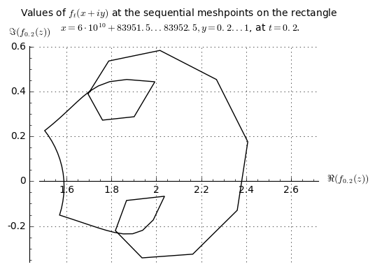
As is constant in this region, the function is holomorphic, so by Rouche’s theorem, it suffices to show that for each time , as traverses the boundary of the rectangle
the function stays outside of the ball , and furthermore has a winding number of zero around the origin.
To verify this claim numerically for a given value of , we subdivide each edge of into some number of equally spaced mesh points, thus approximating by a discrete mesh , , with any two adjacent points on this mesh separated by a distance at most . Using the techniques in Section 7, we evaluate numerically for each such value of . The polygonal path connecting these points then winds around the origin with winding number
which can be easily computed (and verified to be zero). To pass from this polygonal path to the true trajectory of on , we again use Rouche’s theorem. If one has a derivative bound on the boundary of the rectangle, the polygonal path and the true trajectory differ by a distance of at most , and the latter will have the same winding number around the origin (and stay outside of the ball ) as long as
Furthermore, the same is true for nearby times to , as long as one has the stronger bound
| (91) |
and a bound of the form for and .
This gives the following algorithm to verify (a) for the entire range . We start with and obtain bounds for the derivatives of in the indicated ranges. Because of the way the barrier location was selected, we expect to stay well above in magnitude. We thus choose so that , and evaluate at all the mesh points (in particular confirming that does stay well above ). Using the minimum value of , we can then use the condition (91) to establish the claim for times in the interval where is chosen so that (91) holds (or , if that is also possible); the most aggressive choice of would be one in which (91) held with equality, but in practice we can afford to take more conservative values of and still obtain good runtime performance. If , we then repeat the process, replacing by , until the entire range is verified.
To run this algorithm, we need bounds on and . This is achieved by the following lemma, which gives bounds which are somewhat complicated but which can be easily upper bounded numerically on :
Lemma 8.4.
Proof.
We begin with the first estimate. Write
then
| (92) |
One can check that are holomorphic functions of , hence by the Cauchy-Riemann equations
By the product and chain rules, we may calculate
Similarly we have
Writing , we have from (16), (10) that
and hence by (8)
From the triangle inequality and (43), we thus have
We have from (9) that
since . Similarly
and thus
Writing , we then have the first estimate.
The next few graphs summarize the numerical output of the algorithm for the following barrier parameters: .
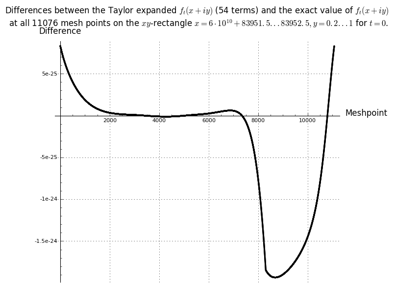
The first step in the barrier verification process was to precalculate a ‘stored sum’ of Taylor expansion terms that allows for fast recreation of during the execution of the algorithm as per Section 7. The number of Taylor terms required was determined through an iterative process targeted to achieve a decimal accuracy. Figure 13 illustrates that the achieved accuracy for all rectangular mesh points at .
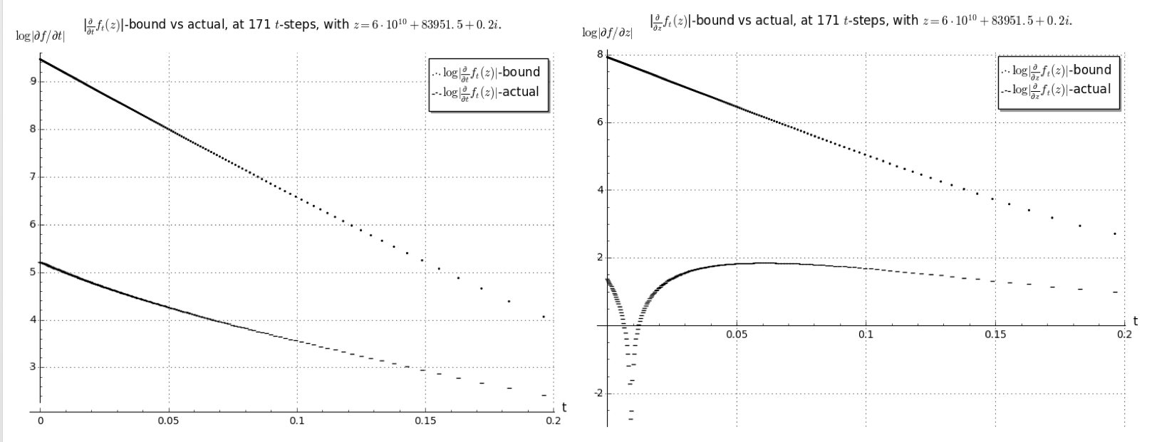
The derivative bounds determine the number of mesh points required on each -rectangle and in the -direction. Figure 14 illustrates that these bounds have been chosen quite conservatively:
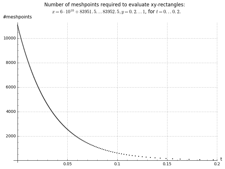
The number of rectangle mesh points varies with ranging from at to at ; see Figure 15.
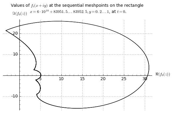
The overall winding number for the barrier at this specific location came out at . Figures 16, 17 show the winding process at respectively. Due to the choice of the barrier location and the small barrier width compared to the wavelength in the variable, little oscillation is expected to occur in each rectangle.
The code for implementing these computations may be found in the directory
dbn_upper_bound/arb
in the github repository [20].
8.5. Proof of claim (b)
Fix , and let denote the rectangle
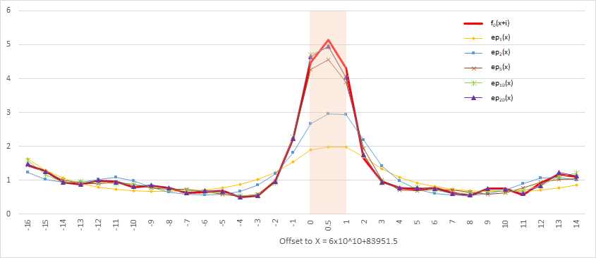
We wish to show that the holomorphic function does not vanish in this rectangle. We would like to establish this by the argument principle, however this turns out to be difficult to accomplish due to the oscillation in indicated by the heuristic (79). To damp out this oscillation, we introduce an777In the literature one also sees other choices of mollifier than this Euler product used, for instance to control the extreme values of Dirichlet polynomials; however our numerical experimentations with alternative mollifiers to turned out to give inferior results for our application. “Euler mollifier”
where is given by (17) the choice to use the first three primes was obtained after significant trial and error as giving the best numerical results in this range of . We have the upper bound
When , and , one easily verifies from (21) that
and hence
In particular, by Proposition 8.1 we have
The left-hand side remains holomorphic in (even though has jump discontinuities). Thus, by the argument principle, it will suffice to show that the left-hand side avoids the negative real axis as traverses the boundary of the rectangle . In other words, it will suffice to show that
| (93) |
for . For future reference we also observe that for any , the magnitude of can be bounded below by
| (94) |
and the argument has magnitude at most
| (95) |
Of the four sides of the rectangle , the required estimate (93) will hold with significant room to spare, and we can proceed using rather crude estimates. We first attend to the right edge of , in which . From (88) we have
in this region. In particular has argument of magnitude at most . Combining this with (94), (95), we conclude that has magnitude at least and argument at most in magnitude, giving the claim (93) on this side from elementary trigonometry.
Now we attend to the left edge of , in which and . From the calculations for part (a) (see in particular Figure 17) one can verify that (for instance) and in this region. Combining this with (94), (95), we conclude that has magnitude at least and argument at most in magnitude, again giving the claim (93) on this side from elementary trigonometry.
Now we attend to the upper edge of , in which and . From (21) one now has
In particular888The sum can be numerically computed directly, but one could also use Lemma 8.2 (using for instance ) to obtain a usable upper bound as well. Similarly for the other sums of this type that appear in this argument.
Meanwhile, from (20) one has
and from (22) one has
and hence
and
and hence
In particular has magnitude at least and argument at most in magnitude, hence has magnitude at least and argument at most , at which point the claim follows from elementary trigonometry.
It remains to attend to the lower edge of , in which and . This is by far the most delicate side of the rectangle for the purposes of verifying (93). We will split the range into a number of subintervals and obtain a uniform lower bound for when is in one of these subintervals .
Fix , suppose that , and write . We first deal with the term in the definition of by writing
and hence
| (96) |
In particular, using (20) to bound
we have
where
We can write
where and
As a consequence, we have
where
Thus for instance and for , so that the Dirichlet series is expected to experience less oscillation than the series .
The product of and is not favorable due to the negative sign in the exponent. But since , we have
where
Note that the coefficients are both real. We now have
| (97) |
A naive application of the triangle inequality (using ) would give the lower bound
| (98) |
As it turns out, this bound is not quite strong enough to be satisfactory for the numerical ranges of parameters we need. To do better we need to exploit the fact that when the sum exhibits significant cancellation, then the sum will also. The key tool here is
Lemma 8.5 (Improved triangle inequality).
We have
Proof.
Write
We may assume that , otherwise the claim is trivial. By (97) and convexity, it suffices to show that
for all phases . We may write
By the cosine rule, we have
This is a fractional linear function of with no poles in the range of . Thus this function is monotone on this range and attains its maximum at either or . We conclude that
and thus
We conclude from the triangle inequality that
By further application of the triangle inequality
as desired, where we have used the fact that lies to the right of the imaginary axis (so that the closest element of is the origin). ∎
Bounding , we see that in order to establish (93) in the range , it suffices to verify the inequality
where
and hence it suffices to show that
where
and
Since , we may crudely bound
so it will suffice to show that
for a collection of intervals covering . This can be done by ad hoc numerical experimentation; for instance, one can calculate that
9. Asymptotic results
In this section we use the effective estimates from Theorem 1.3 to obtain asymptotic information about the function , which improves (and makes more effective) the results of Ki, Kim, and Lee [10], by establishing Theorem 1.5.
We begin with
Proposition 9.1 (Preliminary asymptotics).
Let , , and .
-
(i)
If for a sufficiently large absolute constant , then
for an absolute constant , where is defined in (10).
-
(ii)
If instead we have and for a sufficiently large absolute constant , then
-
(iii)
If for some , then
Proof.
We begin with (i). Since and , we may assume without loss of generality that . Using (16), (11) we may write the desired estimate as
We apply Theorem 1.3. (Strictly speaking, the estimates there required rather than ; however, as remarked at the beginning of Section 6, all the estimates in that section would continue to hold under this weaker hypothesis if one adjusted all the numerical constants appropriately.) This gives
| (99) |
where
Since , we have and for all . We conclude that
so it will suffice (for small enough) to show that
By (15) we can write the left-hand side as
For , we have
for some absolute constant . By the integral test, the left-hand side is then bounded by
which, for and large, is bounded by . The claim then follows after adjusting appropriately.
Now we prove (ii). As before we have the expansion (99). We have
similar arguments give , while
We conclude that
as claimed, if for large enough.
To understand the behavior of , we make the following simple observations:
Lemma 9.2 (Behavior of ).
Let , let be sufficiently large, and let . Then
Also, there is a continuous branch of for all large real such that
Proof.
By (10), (8), the log-derivative of is given by
| (100) |
For , we have from (9) that
| (101) |
and from this and (43) we conclude that
whenever . The first claim then follows by applying the fundamental theorem of calculus to a branch of .
For the second claim, we calculate
as desired. ∎
Now we can prove Theorem 1.5. We begin with (ii). Let , and suppose that . By Proposition 9.1(i) and Lemma 9.2 we have
| (102) |
From Lemma 9.2 and (26) one has
and hence
| (103) |
If we now make the further assumption , we can thus simplify the above approximation as
| (104) |
In particular, if traverses the circle once anti-clockwise and is small enough, the quantity will wind exactly once around the origin, and hence by the argument principle there is precisely one zero of inside this circle. As the zeroes of are symmetric around the real axis, this zero must be real. This proves (ii).
Now we prove (i). Suppose that and . We can assume since it is known (e.g., from [5, Theorem 13]) that there are no zeroes with .
Let be a natural number that minimises , then since the derivative of the left-hand side of (26) in is comparable to . From (102) we have
Thus both summands on the right-hand side have the same magnitude, which on taking logarithms and canceling like terms implies that
and hence . We can now apply (104) to conclude that
which (when combined with the hypothesis that is minimal) forces . This gives the claim.
Next, we prove (iii). In view of parts (i) and (ii), and adjusting if necessary, we may assume that takes the form for some . By the argument principle, is equal to times the variation in the argument of on the boundary of the rectangle traversed clockwise, since there are no zeroes with imaginary part of magnitude greater than one. By compactness, the variation on the left edge is , and similarly for any fixed portion of the upper edge. From Proposition 9.1 (and (102)), we see that the variation of on the remaining upper edge and on the top half of the right edge are both equal to . Since , the variation on the lower half of the rectangle is equal to that of the upper half. We thus conclude that
where we use a continuous branch of the argument of that is bounded at . The claim now follows from Lemma 9.2 (using to work with instead of ).
Finally, we prove (iv). From the Hadamard factorization theorem as in the proof of Proposition 3.1 we have
| (105) |
where the zeroes of are indexed in pairs . Setting , we see from Proposition 9.1 and the generalized Cauchy integral formula that the logarithmic derivative of is equal to at for all sufficiently large , and hence for all by symmetry and compactness. On the other hand, from Stirling’s formula (or the logarithmic growth of the digamma function) one easily verifies that the logarithmic derivative of is equal to at . Hence . Taking imaginary parts, we conclude that
where we write ; equivalently one has
where the sum now ranges over all zeroes, including any at the origin. Since , every zero in makes a contribution of at least (say). As the summands are all positive, the first part of claim (iv) follows. To prove the second part, we may assume by compactness that . Repeating the proof of (iii), and reduce to showing that the variation of on the short vertical interval is . If we let be a phase such that is real and positive, we see that this variation is at most , where is the number of zeroes of for , since every increment of in must be accompanied by at least one such zero. As , this is also the number of zeroes of . On the other hand, from Proposition 9.1(ii), (iii) and Jensen’s formula we see that the number of such zeroes is , and the claim follows.
Remark 9.3.
Theorem 1.5 gives good control on whenever . As a consequence (and assuming for sake of argument that the Riemann hypothesis holds), then for any , the bound should be numerically verifiable in time , by applying the arguments of previous sections with and set equal to small multiples of . We leave the details to the interested reader.
Remark 9.4.
Our discussion here will be informal. In view of the results of [9], it is expected that the zeroes of should evolve according to the system of ordinary differential equations
where the sum is evaluated in a suitable principal value sense, and one avoids those times where the zero fails to be simple; see [9, Lemma 2.4] for a verification of this in the regime . In view of the Riemann-von Mangoldt formula (as well as variants such Corollary 1.5, it is expected that the number of zeroes in any region of the form for large should be of the order of . As a consequence, we expect a typical zero to move with speed , although one may occasionally move much faster than this if two zeroes are exceptionally close together, or less than this if the zeroes are close to being evenly spaced. As a consequence, if the Riemann hypothesis fails and there is a zero of with comparable to , it should take time comparable to for this zero to move towards the real axis, leading to the heuristic lower bound . Thus, in order to obtain an upper bound , it will probably be necessary to verify that there are no zeroes of with comparable to and for some small absolute constant . This suggests that the time complexity bound in Remark 9.3 is likely to be best possible (unless one is able to prove the Riemann hypothesis, of course).
In [9, Lemma 2.1] it is also shown that the velocity of a given zero is given by the formula
assuming that the zero is simple. By using the asymptotics in Proposition 9.1 and Corollary 1.5 together with the generalized Cauchy integral formula to then obtain asymptotics for and , it is possible to show that for the zeroes that are real and larger than , and move leftwards with velocity
we leave the details to the interested reader.
10. Further numerical results
By Theorem 1.5, one can verify the second hypothesis of Theorem 1.2 when for a large constant . If we ignore for sake of discussion the third hypothesis of Theorem 1.2 (which turns out to be relatively easy to verify numerically in practice), this suggests that one can obtain a bound of the form provided that one can verify the Riemann hypothesis up to a height . In other words, if one has numerically verified the Riemann hypothesis up to a large height , this should soon lead to a bound of the form .
Aside from improving the implied constant in this bound, it does not seem easy to improve this sort of implication without a major breakthrough on the Riemann hypothesis (such as a massive expansion of the known zero-free regions for the zeta function inside the critical strip). We shall justify this claim heuristically as follows. Suppose that there was a counterexample to the Riemann hypothesis at a large height , so that for some positive , which for this discussion we will take to be comparable to . The Riemann von Mangoldt formula indicates that the number of zeroes of within a bounded distance of this zero should be comparable to ; the majority of these zeroes should obey the Riemann hypothesis and thus stay at roughly unit distance from our initial zero . Proposition 3.1 then suggests that as time advances, this zero should move at speed comparable to . Thus one should not expect this zero to reach the real axis until a time comparable to . This heuristic analysis therefore indicates that it is unlikely that one can significantly improve the bound without being able to exclude significant violations of the Riemann hypothesis at height .
The table below collects some numerical results verifying the second two hypotheses of Theorem 1.2 for larger values of , and smaller values of , than were considered in Section 8. This leads to improvements to the bound conditional on the assumption that the Riemann Hypothesis can be numerically verified beyond the height used in Section 8. For instance, the final row of the table implies that one has the bound assuming that the Riemann hypothesis is verified up to the height . Note that this is broadly consistent with the previous heuristic that the upper bound on is proportional to .
| Winding Number | lower bound | |||||
|---|---|---|---|---|---|---|
| 0.198 | 0.15492 | 0.21 | 0 | 398942 | 0.0341 | |
| 0.186 | 0.16733 | 0.20 | 0 | 630783 | 0.0376 | |
| 0.180 | 0.14142 | 0.19 | 0 | 1261566 | 0.0349 | |
| 0.168 | 0.15492 | 0.18 | 0 | 2185096 | 0.0377 | |
| 0.161 | 0.13416 | 0.17 | 0 | 4886025 | 0.0369 | |
| 0.153 | 0.11832 | 0.16 | 0 | 12615662 | 0.0532 | |
| 0.139 | 0.14832 | 0.15 | 0 | 23601743 | 0.0350 | |
| 0.132 | 0.12649 | 0.14 | 0 | 69098829 | 0.0307 | |
| 0.122 | 0.12649 | 0.13 | 0 | 218509686 | 0.0347 | |
| 0.113 | 0.11832 | 0.12 | 0 | 846284375 | 0.0318 | |
| 0.102 | 0.12649 | 0.11 | 0 | 3989422804 | 0.0305 | |
| 0.093 | 0.11832 | 0.1 | 0 | 26761861742 | 0.0321 |
The selection of parameters in this table proceeded as follows. One first located parameters (with the quantity as small as possible) for which one could obtain a good lower bound for when ; we arbitrarily chose a target lower bound of to provide an adequate safety margin. From (96) one had
| (106) |
where
and
The final term on the right-hand side of (106) can be estimated as in Section 8.5 and is negligible in practice. To control the other two terms, we use the following lemma (which roughly speaking corresponds to a simplified version of the “Euler 2 mollifier” version of the “Euler 5 mollifier” analysis in Section 8.5):
Lemma 10.1.
Let be complex numbers, and let be a number such that whenever is even, lies on the line segment connecting 0 with . Then we have the lower bound
and the upper bound
Proof.
The quantity can be written as
By the triangle inequality, this is bounded above by
and below by
We have
which we can rearrange as
and the claim follows. ∎
Using this lemma to lower bound and upper bound , and then using the triangle inequality, yields a lower bound on when . These quantities can be readily computed for many values of , leading to an envelope for and that is depicted in Figure 20.
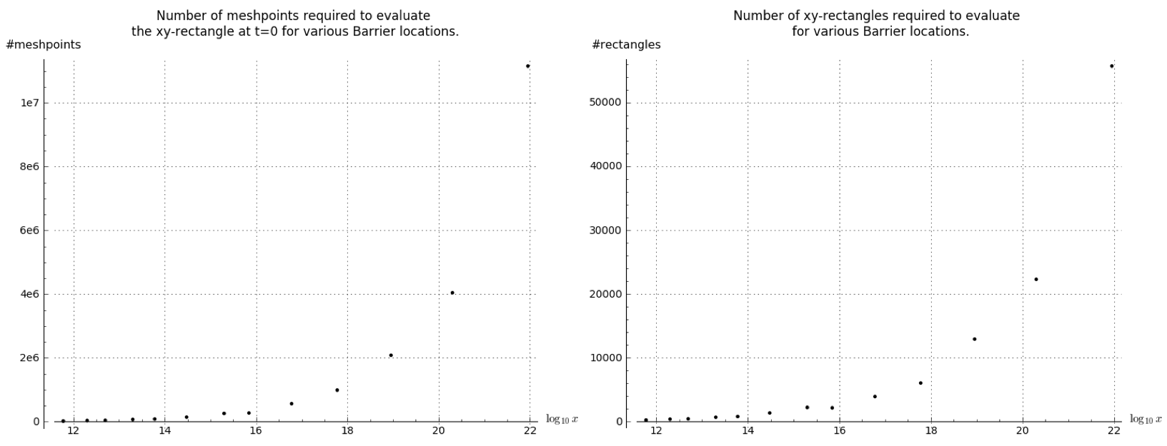
By working in intervals for some finite number of intervals covering for some large as in Section 8.5, and then using a crude triangle inequality bound for as in Section 8.3, we thus (in view of the conservative safety margin in our lower bounds for ) expect to be able to verify the hypothesis in Theorem 1.2(iii) for any choice of parameters as above. The main remaining difficulty is then to verify the barrier hypothesis (Theorem 1.2(ii)). This is by far the most numerically intensive step, and we proceed as in Section 8.4, after using the ad hoc procedure in Section 8.1 to select . The graphs in figure 21 illustrate that for increasing , the number of xy-rectangles to be evaluated within the barrier, as well as the number of mesh points required per rectangle (measured at ), increase exponentially.
All barrier runs generated a winding number of zero for each rectangle and the scripts completed successfully without any errors. For all barrier locations, the computations of the mesh points where calculated at digits accuracy except for the highest two where digits where used (to be able to compute it within a reasonable time). Checks where made before each formal run to assure the target accuracy would be achieved.
The computations for and in the above table were massive, and performed using a Boinc [1] based grid computing setup, in which a few hundred volunteers participated. Their contributions can be tracked at anthgrid.com/dbnupperbound.
11. Conflict of interest statement
There are no conflicts of interest for this paper.
References
- [1] D. P. Anderson, BOINC: A System for Public-Resource Computing and Storage, In GRID ’04: Proceedings of the Fifth IEEE/ACM International Workshop on Grid Computing (2004), 4–10.
- [2] J. Arias de Reyna, High-precision computation of Riemann’s zeta function by the Riemann-Siegel asymptotic formula, I, Mathematics of Computation, 80 (2011), 995–1009.
- [3] J. Arias de Reyna, J. Van de lune, On the exact location of the non-trivial zeroes of Riemann’s zeta function, Acta Arith. 163 (2014), 215–245.
- [4] W. G. C. Boyd, Gamma Function Asymptotics by an Extension of the Method of Steepest Descents, Proceedings: Mathematical and Physical Sciences, Vol. 447, No. 1931 (Dec. 8, 1994), 609–630.
- [5] N. C. de Bruijn, The roots of trigonometric integrals, Duke J. Math. 17 (1950), 197–226.
- [6] G. Csordas, T. S. Norfolk, R. S. Varga, A lower bound for the de Bruijn-Newman constant , Numer. Math. 52 (1988), 483–497.
- [7] G. Csordas, A. M. Odlyzko, W. Smith, R. S. Varga, A new Lehmer pair of zeros and a new lower bound for the De Bruijn-Newman constant Lambda, Electronic Transactions on Numerical Analysis. 1 (1993), 104–111.
- [8] G. Csordas, A. Ruttan, R.S. Varga, The Laguerre inequalities with applications to a problem associated with the Riemann hypothesis, Numer. Algorithms, 1 (1991), 305–329.
- [9] G. Csordas, W. Smith, R. S. Varga, Lehmer pairs of zeros, the de Bruijn-Newman constant , and the Riemann hypothesis, Constr. Approx. 10 (1994), no. 1, 107–129.
- [10] H. Ki, Y. O. Kim, and J. Lee, On the de Bruijn-Newman constant, Advances in Mathematics, 22 (2009), 281–306.
- [11] D. H. Lehmer, On the roots of the Riemann zeta-function, Acta Math. 95 (1956), 291–298.
- [12] H. L. Montgomery, The pair correlation of zeros of the zeta function, Analytic number theory (Proc. Sympos. Pure Math., Vol. XXIV, St. Louis Univ., St. Louis, Mo., 1972), 181–193. Amer. Math. Soc., Providence, R.I., 1973.
- [13] H. L. Montgomery, R. C. Vaughan, Multiplicative number theory. I. Classical theory. Cambridge Studies in Advanced Mathematics, 97. Cambridge University Press, Cambridge, 2007.
- [14] C. M. Newman, Fourier transforms with only real zeroes, Proc. Amer. Math. Soc. 61 (1976), 246–251.
- [15] T. S. Norfolk, A. Ruttan, R. S. Varga, A lower bound for the de Bruijn-Newman constant II., in A. A. Gonchar and E. B. Saff, editors, Progress in Approximation Theory, 403–418. Springer-Verlag, 1992.
- [16] A. M. Odlyzko, An improved bound for the de Bruijn-Newman constant, Numerical Algorithms 25 (2000), 293–303.
- [17] T. K. Petersen, Eulerian numbers. With a foreword by Richard Stanley. Birkhäuser Advanced Texts: Basler Lehrbücher. Birkhäuser/Springer, New York, 2015.
- [18] D. J. Platt, Isolating some non-trivial zeros of zeta, Math. Comp. 86 (2017), 2449–2467.
- [19] G. Polya, Über trigonometrische Integrale mit nur reelen Nullstellen, J. Reine Angew. Math. 58 (1927), 6–18.
- [20] D. H. J. Polymath, github.com/km-git-acc/dbn_upper_bound
- [21] D. H. J. Polymath, Zeroes of the heat flow evolution of the Riemann function at negative times: numerical experiments and heuristic justifications, github.com/km-git-acc/dbn_upper_bound/blob/master/Writeup/Sharkfin/sharkfin.pdf
- [22] B. Rodgers, T. Tao, The De Bruijn-Newman constant is nonnegative, preprint. arXiv:1801.05914
- [23] Y. Saouter, X. Gourdon, P. Demichel, An improved lower bound for the de Bruijn-Newman constant, Mathematics of Computation. 80 (2011), 2281–2287.
- [24] J. Stopple, Notes on Low discriminants and the generalized Newman conjecture, Funct. Approx. Comment. Math., vol. 51, no. 1 (2014), 23–41.
- [25] J. Stopple, Lehmer pairs revisited, Exp. Math. 26 (2017), no. 1, 45–53.
- [26] H. J. J. te Riele, A new lower bound for the de Bruijn-Newman constant, Numer. Math., 58 (1991), 661–667.
- [27] E. C. Titchmarsh, The Theory of the Riemann Zeta-function, Second ed. (revised by D. R. Heath-Brown), Oxford University Press, Oxford, 1986.