NuOscProbExact: a general-purpose code to compute
exact two-flavor and three-flavor neutrino oscillation probabilities

Abstract

In neutrino oscillations, a neutrino created with one flavor can be later detected with a different flavor, with some probability. In general, the probability is computed exactly by diagonalizing the Hamiltonian operator that describes the physical system and that drives the oscillations. Here we use an alternative method developed by Ohlsson & Snellman to compute exact oscillation probabilities, that bypasses diagonalization, and that produces expressions for the probabilities that are straightforward to implement. The method employs expansions of quantum operators in terms of SU(2) and SU(3) matrices. We implement the method in the code NuOscProbExact, which we make publicly available. It can be applied to any closed system of two or three neutrino flavors described by an arbitrary time-independent Hamiltonian. This includes, but is not limited to, oscillations in vacuum, in matter of constant density, with non-standard matter interactions, and in a Lorentz-violating background.

I Introduction

Neutrinos are created and detected in weak interactions as flavor states — $\nu_{e}$, $\nu_{\mu}$, $\nu_{\tau}$ — but they propagate as superpositions of propagation states — in vacuum, these are the mass eigenstates $\nu_{1}$, $\nu_{2}$, $\nu_{3}$. Because the superposition evolves with time, a neutrino created with a certain flavor has a non-zero probability of being detected later with a different flavor Pontecorvo (1968); Barger et al. (1980a); Bilenky (2004); Fantini et al. (2018). The observation of oscillations in solar, atmospheric, reactor, and accelerator neutrinos has led to the momentous discovery of neutrino mass and of flavor mixing in leptons Kajita (2016); McDonald (2016).

Computing the probabilities of flavor transition is integral to studying oscillations. Computing them exactly typically involves diagonalizing the Hamiltonian operator that drives the time-evolution of neutrinos. But, because the expressions involved are often complex, it is notoriously hard to produce exact analytical expressions for the probabilities that also provide physical insight. The case of oscillations in vacuum is an exception Kayser (1981); Giunti and Kim (2007); Tanabashi et al. (2018). Beyond that, there is a large body of work dedicated to deriving exact probabilities for different scenarios; see, e.g., Refs. Barger et al. (1980b); Petcov (1988); Zaglauer and Schwarzer (1988); Torrente Luján (1996); Balantekin (1998); Coleman and Glashow (1999); Gago et al. (2001); Kimura et al. (2002); Harrison et al. (2003); Kostelecky and Mewes (2004a, b); González-García and Maltoni (2004); Blennow and Ohlsson (2004); Meloni et al. (2009); Ando et al. (2009); Abe et al. (2015); Flores and Miranda (2016); Popov and Studenikin (2018). Yet, though some of these expressions are superficially elegant, they are seldom used due to their underlying complexity, particularly in the case of oscillations amongst three neutrino flavors.

More often, carefully selected perturbative expansions and approximations are employed to cast the probabilities in forms that are amenable to physical interpretation. Many such approximate expressions exist in the literature Gago et al. (2002); Blennow and Ohlsson (2008); Díaz et al. (2009); Meloni et al. (2009); Esteves Chaves et al. (2018), especially for oscillations in matter Petcov and Toshev (1987); Hirota (1998); Cervera et al. (2000); Freund (2001); Akhmedov et al. (2004); Friedland and Lunardini (2006); Ioannisian and Smirnov (2009); Supanitsky et al. (2008); Minakata and Parke (2016); Flores and Miranda (2016); Li et al. (2016); Denton et al. (2016); Barenboim et al. (2019) with precisions that reach the per-cent level. Unfortunately, there is no systematic way to produce these useful expressions, since they are tailored to specific Hamiltonians (however, see, LABEL:Denton et al. (2018)), their derivation is not trivial, or their application is limited to specific ranges of values of a perturbative parameter.

Hence, the best course of action in cases where we seek high precision in the computation of probabilities is simply to compute them exactly, often numerically. This is a common strategy to explore non-standard oscillation scenarios, i.e., arbitrary Hamiltonians, for which analytic solutions are in general unavailable. For instance, this is done when scanning a parameter space without knowing a priori our region of interest, or approximate expressions of the probabilities that are valid inside that region.

Here, in lieu of diagonalizing the Hamiltonian, we use an alternative method, developed by Ohlsson & Snellman (hereafter, OS) in Refs. Ohlsson and Snellman (2000a, b); Ohlsson (2000); Ohlsson and Snellman (2001), to compute exact oscillation probabilities. We provide a numerical implementation for systems of two and three neutrino flavors. The method relies on expanding the quantum operators that drive the time-evolution of neutrinos in terms of SU(2) and SU(3) matrices Ohlsson and Snellman (2000a, b); Ohlsson (2000); Ohlsson and Snellman (2001). It has two assumptions:

1. The system must be closed, i.e., it must conserve the number of neutrinos summed over all flavors

2. The Hamiltonian must be time-independent (except in some cases; see Section VI.2)

Both conditions are satisfied in many physical scenarios studied in the literature, e.g., oscillations in vacuum, in matter of constant density, with non-standard neutrino interactions, and in diverse new-physics scenarios. The method does not apply to scenarios where neutrinos “leak out” of the system, e.g., 3+1 systems of sterile neutrinos Abazajian et al. (2012); Palazzo (2013); Gariazzo et al. (2016); Dentler et al. (2018); Giunti and Lasserre (2019), with neutrino decays into invisible products Joshipura et al. (2002); Beacom and Bell (2002); Beacom et al. (2003); González-García and Maltoni (2008); Baerwald et al. (2012); Berryman et al. (2015), or open systems, like those with decoherence Benatti and Floreanini (2000); Lisi et al. (2000); Ohlsson (2001); Carpio et al. (2018); Coloma et al. (2018).

We provide the computer code NuOscProbExact Bustamante , a lightweight numerical implementation of the OS method that computes exact two- and three-flavor oscillation probabilities for arbitrary time-independent Hamiltonians. The code can be easily used in oscillation analyses.

In Section II, we set the scope, context, and approach of the paper. In Section III, we recap the basics of neutrino oscillations and establish the concrete goal of the computation. In Sections IV and V, we present the OS method, in a simplified formulation, for systems of two and three flavors. In Section VI, we describe NuOscProbExact and show examples of its use. In Section VII, we conclude.

II Scope, context, and approach

Below, to compute the oscillation probabilities, we follow the OS method. References Ohlsson and Snellman (2000a, b); Ohlsson (2000); Ohlsson and Snellman (2001) introduced expressions applicable to generic oscillation scenarios, and also found analytic expressions Ohlsson and Snellman (2000a) for the probabilities in the cases of two-flavor oscillations in matter and three-flavor oscillations in vacuum and matter. Reference Barger et al. (1980b) presented an earlier application to three-flavor oscillations in matter. Because the exact analytic expressions tailored to three-neutrino oscillations in vacuum and matter are lengthy, and because we are interested in providing a general-purpose numerical implementation of the method, we do not attempt to reproduce analytical solutions or find new ones.

Later, we work through the method. Here, we give an overview. We start by expanding the Hamiltonian in terms of $2\times 2$ Pauli matrices — in the case of two neutrino flavors — or of $3\times 3$ Gell-Mann matrices — in the case of three flavors. Appendix A shows these matrices. When studying neutrino oscillations, these expansions are sometimes performed not on the Hamiltonian, but on the associated density matrix. This approach is particularly useful to study oscillations in the early Universe McKellar and Thomson (1994); Bell et al. (1999); Hannestad (2002); Wong (2002); Hannestad et al. (2012); Boriero et al. (2017) and in supernovae Pantaleone (1995); Sigl (1995); Pastor and Raffelt (2002); Balantekin and Yuksel (2005); Fogli et al. (2007); Dasgupta and Dighe (2008); Duan et al. (2010); Mirizzi et al. (2016).

In the OS method, we instead first expand the Hamiltonian $H$ and then the associated time-evolution operator $e^{-iHt}$. For the latter, we use the exponential expansions of Pauli and Gell-Mann matrices MacFarlane et al. (1968); Curtright and Zachos (2015); Van Kortryk (2016). These expansions are a direct application of the Cayley-Hamilton theorem, which states that an analytic function of an $n\times n$ matrix can be written as a polynomial of degree $(n-1)$ in that matrix. The coefficients of the expansion are computed using SU(2) and SU(3) invariants, which allows us to bypass the diagonalization of the Hamiltonian that would otherwise be needed to compute the probabilities.

Sophisticated numerical codes exist to compute probabilities, either for general application or for particular scenarios, e.g., GLoBES Huber et al. , nuCraft Wallraff and Wiebusch , NuSQuIDS Argüelles Delgado et al. , and Prob3++ Wendell . The general-purpose code NuSQuIDS Argüelles Delgado et al. (2015, ) implements the same expansions used in the OS method efficiently, and embeds them in a larger formalism that can also deal with time-dependent Hamiltonians. The code Prob3++ Wendell implements the expansions for oscillations in matter, based on LABEL:Barger et al. (1980b).

While it is possible to extend the method to systems of $n>3$ neutrino flavors, the expansions in SU($n$) quickly become complicated Kusnezov (1995); Van Kortryk (2016). Since the objective of NuOscProbExact is to treat the common cases of two- and three-neutrino oscillations, exploring these generalizations is beyond the scope of this paper. However, LABEL:Kamo et al. (2003) applied the OS method to the $n=4$ case for four-flavor oscillations in matter and NuSQuIDS Argüelles Delgado et al. (2015, ) implements it for cases up to $n=6$ Salvadó .

Below, our approach is expository while condensed: we provide sufficient detail to present the method and facilitate its implementation, and refer to earlier works for further mathematical detail.

III Neutrino oscillation recap

Let $\nu$ represent the flavor state of a neutrino. The state evolves according to the Schrödinger equation

$$i\frac{d\nu}{dt}=H\nu\;,$$ (1)

where $t$ is the time elapsed since the creation of the neutrino and $H$ is the Hamiltonian written in flavor space. We use units where $c=\hbar=1$. By definition, $H$ is Hermitian. In a system of $n$ neutrinos, we represent $H$ by a $n\times n$ matrix and $\nu$ by a column vector with $n$ entries. Below, we consider the cases $n=2$, for two-neutrino oscillations, and $n=3$, for three-neutrino oscillations.

We restrict the discussion to time-independent Hamiltonians, so that the corresponding time-evolution operator is $U\left(t\right)=e^{-iHt}$. Hamiltonians of this type describe, for instance, neutrino propagation in vacuum and in matter of constant density. Because neutrinos are relativistic, we approximate the propagated distance $L\simeq t$. Thus, the evolved state of a neutrino born as $\nu_{\alpha}$ ($\alpha=e,\mu,\tau$) is

$$\nu_{\alpha}\left(L\right)=U(L)\nu_{\alpha}=e^{-iHL}\nu_{\alpha}\;.$$ (2)

Since $H$ is Hermitian, the evolution operator $U$ is unitary.

Because the Hamiltonian in flavor space is non-diagonal, i.e., because it mixes flavor states, after propagating for a distance $L$, the neutrino of initial flavor $\nu_{\alpha}$ becomes a superposition of neutrinos of all flavors, each with a different probability amplitude, $\nu_{\beta}^{\dagger}\nu_{\alpha}(L)$ ($\beta=e,\mu,\tau$). The probability of detecting the neutrino with flavor $\beta$ is $P_{\nu_{\alpha}\to\nu_{\beta}}(L)=\lvert\nu_{\beta}^{\dagger}\nu_{\alpha}(L)\rvert^{2}$.

In Eq. (2), to compute the action of the evolution operator, $\nu_{\alpha}$ must be an eigenstate of $H$. Yet, this is typically not the case. Thus, the usual procedure to compute the evolved state is to diagonalize the Hamiltonian in Eq. (2), compute the evolved state in the space spanned by the eigenvectors of the Hamiltonian, and rotate back to flavor space to obtain $\nu_{\alpha}(L)$. These steps are often carried out numerically, especially in the three-neutrino case, because the expressions quickly become unmanageable. There are numerical codes that do this efficiently, e.g., GLoBES Huber et al. ; Kopp (2008); Huber et al. (2007).

Below, we follow instead the OS method, as explained in Section II, implement it numerically, and show results of the implementation.

IV Two-neutrino oscillations

We consider first oscillations between only two neutrino flavors; later, we consider three flavors. This is a good approximation when describing reactor, accelerator, and atmospheric neutrinos. We represent the two-neutrino Hamiltonian operator by a $2\times 2$ matrix $\mathbb{H}_{2}$. The three traceless, Hermitian Pauli matrices $\sigma^{k}$ ($k=1,2,3$) — the generators of the SU(2) algebra — plus the identity matrix $\mathbb{1}$ make up the orthogonal basis of $2\times 2$ matrices. Thus, we expand the Hamiltonian as

$$\mathbb{H}_{2}=h_{0}\mathbb{1}+h_{k}\sigma^{k}\;,$$ (3)

where, here and below, we assume the Einstein convention of summing over repeated indices. The coefficients $h_{0}$ and $h_{k}$ are functions of the components of the Hamiltonian; we show their explicit expressions in Table 1. In the two-neutrino case, the neutrino state at any time is $\nu(L)=f_{\alpha}(L)\nu_{\alpha}+f_{\beta}(L)\nu_{\beta}$, where $f_{\alpha}$ and $f_{\beta}$ are, respectively, the probability amplitudes of measuring the state to be a $\nu_{\alpha}$ or a $\nu_{\beta}$ (with $\alpha\neq\beta$). We represent the neutrino state as a two-component column vector; the pure states are $\nu_{\alpha}=\left(1~{}0\right)^{\rm T}$ and $\nu_{\beta}=\left(0~{}1\right)^{\rm T}$.

Coefficient	Expression
$h_{0}$	$\frac{1}{2}\left[(\mathbb{H}_{2})_{11}+(\mathbb{H}_{2})_{22}\right]$
$h_{1}$	${\rm Re}\left[(\mathbb{H}_{2})_{12}\right]$
$h_{2}$	$-{\rm Im}\left[(\mathbb{H}_{2})_{12}\right]$
$h_{3}$	$\frac{1}{2}\left[(\mathbb{H}_{2})_{11}-(\mathbb{H}_{2})_{22}\right]$

Table 1: Coefficients in the expansion of the two-neutrino Hamiltonian $\mathbb{H}_{2}$ in Eq. (3). The coefficient $h_{0}$ does not take part in the calculation of the flavor-transition probability; we include it here for completeness.

Thus, the evolution operator is $\mathbb{U}_{2}\left(L\right)=e^{-i\mathbb{H}_{2}L}=e^{-i(h_{0}\mathbb{1}+h_{k}\sigma^{k})L}$. We factorize this into $e^{-ih_{0}\mathbb{1}L}e^{-ih_{k}\sigma^{k}L}$. The operator $e^{-ih_{0}\mathbb{1}L}$ introduces a global phase that does not affect the probability, i.e., $e^{-ih_{0}\mathbb{1}L}\nu=e^{-ih_{0}L}\nu$. After discarding it, we are left with $\mathbb{U}_{2}(L)=e^{-ih_{k}\sigma^{k}L}$.

To compute the action of $\mathbb{U}_{2}$, we use a well-known identity of Pauli matrices that generalizes Euler’s formula,

$$e^{\pm ia_{k}\sigma^{k}}=\cos\left(\left|a\right|\right)\pm i\hat{a}_{k}\sigma^{k}\sin\left(\left|a\right|\right)\;,$$ (4)

where $\hat{a}$ is a unit vector in the direction of the vector $a=(a_{1},a_{2},a_{3})$ and $\lvert a\rvert$ is its modulus. So we can write the evolution operator as in LABEL:Ohlsson and Snellman (2000a),

$$\mathbb{U}_{2}\left(L\right)=\cos\left(\left|h\right|L\right)\mathbb{1}-i\frac{\sin\left(\left|h\right|L\right)}{\lvert h\rvert}h_{k}\sigma^{k}\;,$$ (5)

where $\lvert h\rvert^{2}\equiv\lvert h_{1}\rvert^{2}+\lvert h_{2}\rvert^{2}+\lvert h_{3}\rvert^{2}$.

The evolved state $\nu_{\alpha}(L)$ of a neutrino that was created with flavor $\alpha$, i.e., with $f_{\alpha}(0)=1$ and $f_{\beta}(0)=0$, is $\nu_{\alpha}\left(L\right)=\mathbb{U}_{2}(L)\nu_{\alpha}$. After some manipulation, the flavor-transition probability $P_{\nu_{\alpha}\to\nu_{\beta}}(L)=\lvert\nu_{\beta}^{\dagger}\mathbb{U}_{2}(L)\nu_{\alpha}\rvert^{2}$ is

$$P_{\nu_{\alpha}\to\nu_{\beta}}(L)=\frac{\left|h_{1}\right|^{2}+\left|h_{2}\right|^{2}}{\left|h\right|^{2}}\sin^{2}\left(\left|h\right|L\right)\;\;(\alpha\neq\beta)\;,$$ (6)

where $\lvert h_{1}\rvert^{2}+\lvert h_{2}\rvert^{2}=\lvert(\mathbb{H}_{2})_{12}\rvert^{2}$ and $\lvert h\rvert^{2}=\lvert(\mathbb{H}_{2})_{12}\rvert^{2}+\lvert(\mathbb{H}_{2})_{11}-(\mathbb{H}_{2})_{22}\rvert^{2}/4$. Because of the conservation of probability, $P_{\nu_{\alpha}\rightarrow\nu_{\alpha}}\left(L\right)=1-P_{\nu_{\alpha}\rightarrow\nu_{\beta}}\left(L\right)$. Appendix B contains the derivation of Eq. (6). Appendix C shows a simple application to two-flavor oscillations in vacuum. Equation (6) is our final result in the two-neutrino case.

The key to the calculation of Eq. (6) was to expand the time-evolution operator via the Pauli-matrix identity, Eq. (4). Later, in the three-neutrino case, we use an analogous identity for the Gell-Mann matrices.

V Three-neutrino oscillations

Coefficient	Expression
$h_{0}$	$\frac{1}{3}\left[\left(\mathbb{H}_{3}\right)_{11}+\left(\mathbb{H}_{3}\right)_{22}+\left(\mathbb{H}_{3}\right)_{33}\right]$
$h_{1}$	$\text{Re}\left[{\left(\mathbb{H}_{3}\right)_{12}}\right]$
$h_{2}$	$-\text{Im}\left[{\left(\mathbb{H}_{3}\right)_{12}}\right]$
$h_{3}$	$\frac{1}{2}\left[\left(\mathbb{H}_{3}\right)_{11}-\left(\mathbb{H}_{3}\right)_{22}\right]$
$h_{4}$	$\text{Re}\left[{\left(\mathbb{H}_{3}\right)_{13}}\right]$
$h_{5}$	$-\text{Im}\left[{\left(\mathbb{H}_{3}\right)_{13}}\right]$
$h_{6}$	$\text{Re}\left[{\left(\mathbb{H}_{3}\right)_{23}}\right]$
$h_{7}$	$-\text{Im}\left[{\left(\mathbb{H}_{3}\right)_{23}}\right]$
$h_{8}$	$\frac{\sqrt{3}}{6}\left[\left(\mathbb{H}_{3}\right)_{11}+\left(\mathbb{H}_{3}\right)_{22}-2\left(\mathbb{H}_{3}\right)_{33}\right]$

Table 2: Coefficients in the expansion of the three-neutrino Hamiltonian $\mathbb{H}_{3}$ in Eq. (7). The coefficient $h_{0}$ does not take part in the calculation of the flavor-transition probability; we include it here for completeness.

We follow the steps that we used in the two-neutrino case closely. We represent the three-neutrino Hamiltonian by a $3\times 3$ matrix $\mathbb{H}_{3}$. The eight traceless, Hermitian Gell-Mann matrices $\lambda^{k}$ ($k=1,\ldots,8$) — with $\lambda^{k}/2$ the generators of the SU(3) algebra — plus the identity matrix $\mathbb{1}$ make up the orthogonal basis of $3\times 3$ matrices. Thus, we expand the Hamiltonian as

$$\mathbb{H}_{3}=h_{0}\mathbb{1}+h_{k}\lambda^{k}\;,$$ (7)

where $h_{0}$ and $h_{k}$ are now functions of the components of $\mathbb{H}_{3}$; we show their explicit expressions in Table 2. The neutrino state at any time is $\nu(L)=f_{e}(L)\nu_{e}+f_{\mu}(L)\nu_{\mu}+f_{\tau}(L)\nu_{\tau}$, where $f_{e}$, $f_{\mu}$, and $f_{\tau}$ are, respectively, the probability amplitudes of measuring the state to be a $\nu_{e}$, $\nu_{\mu}$, or $\nu_{\tau}$. We represent the neutrino state as a three-component column vector; the pure states are $\nu_{e}=\left(1~{}0~{}0\right)^{\rm T}$, $\nu_{\mu}=\left(0~{}1~{}0\right)^{\rm T}$, and $\nu_{\tau}=\left(0~{}0~{}1\right)^{\rm T}$.

The evolution operator is $\mathbb{U}_{3}\left(L\right)=e^{-i\mathbb{H}_{3}L}=e^{-ih_{0}\mathbb{1}L}e^{-ih_{k}\lambda^{k}L}$. Again, after discarding the global phase, we are left with $\mathbb{U}_{3}\left(L\right)=e^{-ih_{k}\lambda^{k}L}$.

Next we compute the action of $\mathbb{U}_{3}$ on a neutrino state. We wish to expand $\mathbb{U}_{3}$ using an identity for the Gell-Mann matrices that is similar to the identity for the Pauli matrices, Eq. (4), and that allows us to write

$$\mathbb{U}_{3}\left(L\right)=u_{0}\mathbb{1}+iu_{k}\lambda^{k}\;,$$ (8)

where the complex coefficients $u_{0}$ and $u_{k}$ are functions of $L$ and the $h_{k}$. Reference MacFarlane et al. (1968) introduced and demonstrated such an identity; below, we make use of their results, leaving most of the proofs to the reference. See also Refs. Lehrer-Ilamed (1964); Rosen (1971); Torruella (1975); Kusnezov (1995); Curtright and Zachos (2015); Van Kortryk (2016) for further details.

The coefficients in Eq. (8) can be trivially written as $u_{0}=\frac{1}{3}\text{Tr}~{}\mathbb{U}_{3}$ and $u_{k}=-\frac{i}{2}\text{Tr}(\lambda^{k}\mathbb{U}_{3})$; next we unpack these forms. An application of Sylvester’s formula Sylvester (1883) to $3\times 3$ matrices allows us to express the coefficients in terms of the SU(3) invariants

$$L^{2}\left|h\right|^{2}\equiv L^{2}h_{k}h^{k}\;,$$

$$-L^{3}\langle h\rangle\equiv-L^{3}d_{ijk}h^{i}h^{j}h^{k}\;.$$

The tensor $d_{ijk}=\frac{1}{4}\text{Tr}\left(\{\lambda_{i},\lambda_{j}\}\lambda_{k}\right)$, where the brackets represent the anticommutator. It appears in the product law of Gell-Mann matrices and its components are the structure constants of the SU(3) algebra. Table 3 shows all non-zero components.

Next, we solve the characteristic equation of $-h_{k}\lambda^{k}L$, i.e., $\phi^{3}-(L^{2}\left|h\right|^{2})\phi-\frac{2}{3}(-L^{3}\langle h\rangle)=0$. The equation follows from the Cayley-Hamilton theorem, written conveniently in terms of invariants MacFarlane et al. (1968); Curtright and Zachos (2015). Its three latent roots, or eigenvalues, are $\phi_{m}\equiv\psi_{m}L$ ($m=1,2,3$), with

$$\psi_{m}\equiv\frac{2\left|h\right|}{\sqrt{3}}\cos\left[\frac{1}{3}\left(\chi+2\pi m\right)\right]\;,$$ (9)

where $\cos\left(\chi\right)=-\sqrt{3}\langle h\rangle/\lvert h\rvert^{3}$. The step above is key: writing the eigenvalues in terms of the SU(3) invariants allows us to bypass an explicit diagonalization Curtright and Zachos (2015).

Tensor component	Value
$d_{(118)}=d_{(228)}=d_{(338)}$	$\frac{1}{\sqrt{3}}$
$d_{(146)}=d_{(157)}=d_{(256)}=d_{(344)}=d_{(355)}$	$\frac{1}{2}$
$d_{(247)}=d_{(366)}=d_{(377)}$	$-\frac{1}{2}$
$d_{(448)}=d_{(558)}=d_{(668)}=d_{(778)}$	$-\frac{1}{2\sqrt{3}}$
$d_{888}$	$-\frac{1}{\sqrt{3}}$

Table 3: All of the non-zero components of the tensor $d_{ijk}$, defined in the main text. The tensor is completely symmetric in its indices. Here, $i$, $j$, and $k$ can each take integer values between 1 and 8. The notation $\left(ijk\right)$ represents all permutations of the indices in parentheses. A component vanishes if the number of indices in the set $\left\{2,5,7\right\}$ is odd.

With this, the coefficients in Eq. (8) are

$$u_{0}=\frac{1}{3}\sum_{m=1}^{3}e^{iL\psi_{m}}\;,$$ (10)

$$u_{k}=\sum_{m=1}^{3}e^{iL\psi_{m}}\frac{\psi_{m}h_{k}-\left(h\ast h\right)_{k}}{3\psi_{m}^{2}-\left|h\right|^{2}}\;,$$ (11)

where $\left(h\ast h\right)_{i}\equiv d_{ijk}h^{j}h^{k}$. Appendix D contains the derivation of Eq. (11). Using Eqs. (9), (10), and (11), we write the evolution operator concisely as in LABEL:Ohlsson and Snellman (2000a),

$$\mathbb{U}_{3}(L)=\sum_{m=1}^{3}e^{iL\psi_{m}}\left[\mathbb{1}+\frac{\psi_{m}h_{k}-\left(h\ast h\right)_{k}}{3\psi_{m}^{2}-\lvert h\rvert^{2}}\lambda^{k}\right]\;.$$ (12)

Equation 12 was introduced in Refs.Ohlsson and Snellman (2000a, b); Ohlsson (2000), and applied to find analytic expressions of the probabilities in the cases of oscillations in vacuum and matter. For a numerical implementation of Eq. (12) it is convenient to calculate the coefficients $u_{0}$ and $u_{k}$ with Eqs. (10) and (11), and use them to directly expand $\mathbb{U}_{3}$ in Eq. (8). This is the strategy that we adopt in NuOscProbExact Bustamante .

Three-neutrino probability	Expression
$P_{\nu_{e}\to\nu_{e}}$	$\left|u_{0}+iu_{3}+i\frac{u_{8}}{\sqrt{3}}\right|^{2}$
$P_{\nu_{e}\to\nu_{\mu}}$	$\left|iu_{1}-u_{2}\right|^{2}$
$P_{\nu_{e}\to\nu_{\tau}}$	$\left|iu_{4}-u_{5}\right|^{2}$
$P_{\nu_{\mu}\to\nu_{e}}$	$\left|iu_{1}+u_{2}\right|^{2}$
$P_{\nu_{\mu}\to\nu_{\mu}}$	$\left|u_{0}-iu_{3}+i\frac{u_{8}}{\sqrt{3}}\right|^{2}$
$P_{\nu_{\mu}\to\nu_{\tau}}$	$\left|iu_{6}-u_{7}\right|^{2}$
$P_{\nu_{\tau}\to\nu_{e}}$	$\left|iu_{4}+u_{5}\right|^{2}$
$P_{\nu_{\tau}\to\nu_{\mu}}$	$\left|iu_{6}+u_{7}\right|^{2}$
$P_{\nu_{\tau}\to\nu_{\tau}}$	$\left|u_{0}-i\frac{2u_{8}}{\sqrt{3}}\right|^{2}$

Table 4: Exact three-neutrino oscillation probabilities, for an arbitrary time-independent Hamiltonian. The complex coefficients $u_{0}$ and $u_{k}$ are computed in Eqs. (10) and (11).

The evolved state of a neutrino created as $\nu_{\alpha}$ is $\nu_{\alpha}(L)=\mathbb{U}_{3}(L)\nu_{\alpha}$. Therefore, the flavor-transition probability is $P_{\nu_{\alpha}\to\nu_{\beta}}(L)=\lvert\nu_{\beta}^{\dagger}\mathbb{U}_{3}(L)\nu_{\alpha}\rvert^{2}$. Table 4 shows the expressions for the probabilities in terms of the coefficients $u_{0}$ and $u_{k}$. These are our final results in the three-neutrino case.

Because the algebra of Gell-Mann matrices is more complicated than that of Pauli matrices, the identity that expands the exponential of Gell-Mann matrices in Eq. (8) is notoriously more complicated than the identity that expands the exponential of Pauli matrices, Eq. (5). As pointed out by LABEL:MacFarlane et al. (1968), this may seem a disappointing generalization of Eq. (4) to SU(3). However, when constructing an exponential parametrization of SU(3), there is no way to avoid the solution of at least a cubic equation. Regardless, following the procedure above yields exact three-neutrino flavor-transition probabilities for arbitrary time-independent Hamiltonians.

VI Code description and examples

Description.— The code NuOscProbExact that we provide is a lightweight numerical implementation of the OS method described above. It computes exact oscillation probabilities in the often-studied two- and three-flavor cases, for arbitrary time-independent Hamiltonians. (For more than three flavors and time-dependent Hamiltonians, see NuSQuIDS Argüelles Delgado et al. .) NuOscProbExact is fully written in Python 3.7; it is open source, and publicly available in a GitHub repository Bustamante .

The main input to NuOscProbExact is the Hamiltonian matrix $\mathbb{H}_{2}$ or $\mathbb{H}_{3}$, provided as a $2\times 2$ or $3\times 3$ list. The code internally computes the $h_{k}$ coefficients using Table 1 in the two-neutrino case and Table 2 in the three-neutrino case. To compute two-neutrino probabilities, the code evaluates Eq. (6). To compute three-neutrino probabilities, the code evaluates the expressions in Table 4.

Documentation.— Detailed documentation is in the GitHub repository Bustamante , and is bundled with the code.

Examples.— Listing 1 shows a basic code example of how to use NuOscProbExact to compute three-neutrino probabilities in four representative oscillation scenarios: in vacuum, in matter of constant density, with non-standard interactions in matter, and with Lorentz invariance violation. Bundled with the code we provide further examples, also for two-neutrino oscillations.

Below, we introduce each scenario briefly; we do not explore their phenomenology, but we provide references. Following our tenet, we do not derive analytic expression for the probabilities, only numerically evaluate them.

⬇

1import numpy as np

2

3# NuOscProbExact modules

4import oscprob3nu # Core functionality

5import hamiltonians3nu # Sample Hamiltonians

6from globaldefs import * # Constants (in capitals)

7

8energy = 1.e9 # Neutrino energy [eV]

9baseline = 1.3e3 # Baseline [km]

10

11# Vacuum Hamiltonian before multiplying by 1/energy

12# NO: "normal ordering"; IO: inverted ordering

13h_vacuum_energy_indep = hamiltonians3nu.\

14 hamiltonian_3nu_vacuum_energy_independent( \

15 S12_NO_BF, S23_NO_BF,

16 S13_NO_BF, DCP_NO_BF,

17 D21_NO_BF, D31_NO_BF)

18

19# Hamiltonian for oscillations in vacuum

20h_vacuum = np.multiply( 1./energy,

21 h_vacuum_energy_indep)

22

23# Hamiltonian for oscillations in matter

24# VCC_EARTH_CRUST: Potential [eV], density 3 g cm^{-3}

25h_matter = hamiltonians3nu.hamiltonian_3nu_matter( \

26 h_vacuum_energy_indep, energy, VCC_EARTH_CRUST)

27

28# Hamiltonian for non-standard interactions

29# EPS_3 is the list of NSI strength parameters

30# [EPS_EE, EPS_EM, EPS_ET, EPS_MM, EPS_MT, EPS_TT]

31h_nsi = hamiltonians3nu.hamiltonian_3nu_nsi( \

32 h_vacuum_energy_indep, energy, VCC_EARTH_CRUST,

33 EPS_3)

34

35# Hamiltonian for Lorentz-invariance violation

36# LIV parameters: SXI12, SXI23, SXI13, DXICP, B1,

37# B2, B3, LAMBDA

38h_liv = hamiltonians3nu.hamiltonian_3nu_liv( \

39 h_vacuum_energy_indep, energy,

40 SXI12, SXI23, SXI13, DXICP, B1, B2, B3, LAMBDA)

41

42# The routine probabilities_3nu computes probabilities

43for h_matrix in [h_vacuum, h_matter, h_nsi, h_liv]:

44 # CONV_KM_TO_INV_EV converts km to eV^{-1}

45 Pee, Pem, Pet, Pme, Pmm, Pmt, Pte, Ptm, Ptt = \

46 oscprob3nu.probabilities_3nu( \

47 h_matrix,

48 baseline*CONV_KM_TO_INV_EV)

49

50 print("Pee = %6.5f, Pem = %6.5f, Pet = %6.5f" \

51 % (Pee, Pem, Pet))

52 print("Pme = %6.5f, Pmm = %6.5f, Pmt = %6.5f" \

53 % (Pme, Pmm, Pmt))

54 print("Pte = %6.5f, Ptm = %6.5f, Ptt = %6.5f" \

55 % (Pte, Ptm, Ptt))

56 print()

57

58# This returns:

59# Pee = 0.92768, Pem = 0.01432, Pet = 0.05800

60# Pme = 0.04023, Pmm = 0.37887, Pmt = 0.58090

61# Pte = 0.03210, Ptm = 0.60680, Ptt = 0.36110

62

63# Pee = 0.95262, Pem = 0.00623, Pet = 0.04115

64# Pme = 0.02590, Pmm = 0.37644, Pmt = 0.59766

65# Pte = 0.02148, Ptm = 0.61733, Ptt = 0.36119

66

67# Pee = 0.92494, Pem = 0.01758, Pet = 0.05749

68# Pme = 0.03652, Pmm = 0.32524, Pmt = 0.63824

69# Pte = 0.03855, Ptm = 0.65718, Ptt = 0.30427

70

71# Pee = 0.92721, Pem = 0.05299, Pet = 0.01980

72# Pme = 0.05609, Pmm = 0.25288, Pmt = 0.69103

73# Pte = 0.01670, Ptm = 0.69412, Ptt = 0.28917

Listing 1: Code snippet to use NuOscProbExact to compute three-neutrino oscillation probabilities in vacuum, matter of constant density, with non-standard interactions, and with CPT-odd Lorentz-violating background, for fixed neutrino energy $E=1$ GeV and baseline $L=1300$ km. Constants — with variable names in capitals — are pulled from the globaldefs module; see the main text for their values.

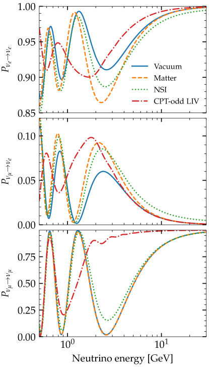
Figure 1: Three-neutrino oscillation probabilities $P_{\nu_{e}\to\nu_{e}}$ (top), $P_{\nu_{\mu}\to\nu_{e}}$ (center), and $P_{\nu_{\mu}\to\nu_{\mu}}$ (bottom), computed using NuOscProbExact Bustamante . The scenarios shown are for oscillations in vacuum, in matter of constant density, with non-standard interactions (NSI), and in a CPT-odd Lorentz-violating background (LIV). In all cases, the baseline is $L=1300$ km. See the main text for details.

Figure 1 shows the probabilities $P_{\nu_{e}\to\nu_{e}}$, $P_{\nu_{\mu}\to\nu_{e}}$, and $P_{\nu_{\mu}\to\nu_{\mu}}$ for the four scenarios, as a function of neutrino energy, computed using NuOscProbExact Bustamante . We set the baseline to $L=1300$ km to match that of the far detector of the planned DUNE experiment Abi et al. (2018). The parameters and their values used in each example case are introduced below. All of the Hamiltonians below are written in the flavor basis. Figure 1 can be generated by running the bundled example file oscprob3nu_plotpaper.py.

Appendix E shows the two-neutrino counterparts of the example three-neutrino scenarios presented below. We provide implementations of these two-neutrino scenarios as part of NuOscProbExact Bustamante .

VI.1 Oscillations in vacuum

The Hamiltonian that drives oscillations in vacuum is

$$\mathbb{H}_{3}^{\rm vac}(E)=\frac{1}{2E}\left(\mathbb{R}_{3,\theta}\mathbb{M}_{3}^{2}\mathbb{R}_{3,\theta}^{\dagger}\right)\;,$$ (13)

where $\mathbb{M}_{3}^{2}\equiv{\rm diag}(0,\Delta m_{21}^{2},\Delta m_{31}^{2})$ is the mass matrix, with $\Delta m_{21}^{2}\equiv m_{2}^{2}-m_{1}^{2}$ and $\Delta m_{31}^{2}\equiv m_{3}^{2}-m_{1}^{2}$, and the $3\times 3$ complex rotation matrix $\mathbb{R}_{3,\theta}$ is the Pontecorvo-Maki-Nakagawa-Sakata (PMNS) mixing matrix. We express it in terms of three mixing angles, $\theta_{13}$, $\theta_{12}$, $\theta_{23}$, and one CP-violation phase, $\delta_{\rm CP}$ Tanabashi et al. (2018).

To compute the probabilities in Fig. 1, we fix the mixing parameters to their best-fit values provided by the recent NuFit 4.0 global fit to oscillation data Esteban et al. (2019); NuFit , assuming normal mass hierarchy, and including Super-Kamiokande atmospheric neutrino data: $\sin^{2}\theta_{12}=0.310$, $\sin^{2}\theta_{23}=0.582$, $\sin^{2}\theta_{13}=0.02240$, $\delta_{\rm CP}=217^{\circ}$, $\Delta m_{21}^{2}=7.39\cdot 10^{-5}$ eV², $\Delta m_{31}^{2}=2.525\cdot 10^{-3}$ eV².

VI.2 Oscillations in matter of constant density

When neutrinos propagate in matter, $\nu_{e}$ and $\bar{\nu}_{e}$ scatter on electrons via charged-current interactions. The interactions introduce potentials that shift the energies of the neutrinos. As a result, the values of the mass-squared differences and mixing angles in matter differ from their values in vacuum, and depend on the number density of electrons Wolfenstein (1978); Mikheyev and Smirnov (1985); Bethe (1986); Parke (1986); Rosen and Gelb (1986). Computing oscillation probabilities in constant matter is integral to long-baseline experiments, where neutrinos traverse hundreds of kilometers in the crust of the Earth to reach the detectors Feldman et al. (2013); Diwan et al. (2016).

The Hamiltonian that drives oscillations in matter is

$$\mathbb{H}_{3}^{\rm matt}(E)=\mathbb{H}_{3}^{\rm vac}(E)+\mathbb{A}_{3}\;.$$ (14)

The term $\mathbb{A}_{3}\equiv{\rm diag}(V_{\rm CC},0,0)$ is due to interactions with matter, where $V_{\rm CC}=\sqrt{2}G_{\rm F}n_{e}$ is the charged-current potential and $n_{e}$ is the number density of electrons.

To compute the probabilities for oscillations in matter (and also with non-standard interactions) in Fig. 1, we consider a constant matter density of $\rho=3$ g cm^-3, the average density of the crust of the Earth Dziewonski and Anderson (1981). The number density of electrons is $n_{e}=Y_{e}\rho/[(m_{p}+m_{n})/2]$, where $m_{p}$ and $m_{n}$ are the masses of the proton and neutron, respectively, and $Y_{e}=0.5$ is the average electron fraction in the crust, which is electrically neutral. See Refs. Ohlsson and Snellman (2000a, b) for the analytic form of the probabilities in matter, deduced with the OS method, and LABEL:Freund (2001) for a related approximation. In long-baseline experiments, even if there are density changes along the trajectory of the neutrino beam, using the average density is a good approximation Petcov (1998); Freund et al. (2000).

The result above can be extended to the case where neutrinos traverse multiple slabs of matter, each of constant, different density. See, e.g., Refs. Chizhov and Petcov (1999, 2001), for an overview of this scenario, and Refs. Ohlsson and Snellman (2000b, 2001); Merfeld and Latimer (2014) for studies with the OS method. This applies to long-baseline neutrino experiments that consider a non-uniform matter density profile Jacobsson et al. (2002); Ohlsson and Winter (2003); Argüelles et al. (2015a); Roe (2017); Kelly and Parke (2018), and to Earth-traversing neutrinos that cross multiple density layers inside Earth Freund and Ohlsson (2000). The probability amplitudes obtained after traversing each slab need to be stitched together Giunti and Kim (2007). If a neutrino created as $\nu_{\alpha}$ traverses $N_{\rm slabs}$ slabs of constant-density matter, each of width $L_{j}$, then the evolved state is $\nu_{\alpha}(\left\{L_{j}\right\})=\left[\prod_{j=1}^{\rm N_{\rm slabs}}\mathbb{U}_{3}^{(j)}(L_{j})\right]\nu_{\alpha}$, where $\mathbb{U}_{3}^{(j)}$ is Eq. (12) computed using the matter Hamiltonian evaluated with the matter density of the $j$-th slab. The final oscillation probability is $P_{\nu_{\alpha}\to\nu_{\beta}}(\left\{L_{j}\right\})=\lvert\nu_{\beta}^{\dagger}\nu_{\alpha}(\left\{L_{j}\right\})\rvert^{2}$.

VI.3 Oscillations with non-standard interactions

Oscillations in matter might receive sub-leading contributions due to new neutrino interactions with the fermions of the medium that they propagate in. These are known as non-standard interactions (NSI); see Refs. Ohlsson (2013); Miranda and Nunokawa (2015); Farzan and Tórtola (2018); Esteban et al. (2018) for reviews.

In this case, the Hamiltonian is

$$\mathbb{H}_{3}^{\rm NSI}(E)=\mathbb{H}_{3}^{\rm vac}(E)+\mathbb{A}_{3}+\mathbb{V}_{3}\;,$$ (15)

where $\mathbb{V}_{3}\equiv V_{\rm CC}\epsilon_{3}$ is the matter potential due to NSI and $\epsilon_{3}$ is the matrix of NSI strength parameters, i.e.,

$$\epsilon_{3}=\left(\begin{array}[]{ccc}\epsilon_{ee}&\epsilon_{e\mu}&\epsilon_{e\tau}\\ \epsilon_{e\mu}^{\ast}&\epsilon_{\mu\mu}&\epsilon_{\mu\tau}\\ \epsilon_{e\tau}^{\ast}&\epsilon_{\mu\tau}^{\ast}&\epsilon_{\tau\tau}\\ \end{array}\right)\;.$$ (16)

The parameters $\epsilon_{\alpha\beta}$ represent the total strength of the NSI between leptons of flavors $\alpha$ and $\beta$ interacting with the electrons, $u$ quarks, and $d$ quarks that make up standard matter. Following LABEL:Esteban et al. (2018), we write $\epsilon_{\alpha\beta}=\epsilon_{\alpha\beta}^{e}+(2+Y_{n})\epsilon_{\alpha\beta}^{u}+(1+2Y_{n})\epsilon_{\alpha\beta}^{d}$, with the ratio of the number densities of neutrons to electrons $Y_{n}\equiv n_{n}/n_{e}\approx 1$ in the Earth. In our simplified treatment, we do not consider separately interactions with each fermion type or each chiral projection of the fermion Ohlsson (2013); Miranda and Nunokawa (2015); Farzan and Tórtola (2018); Esteban et al. (2018).

To compute the probabilities for NSI in Fig. 1, we again consider propagation in the constant-density crust of the Earth, with $V_{\rm CC}$ evaluated as in Section VI.2. Because NSI have not been observed, we choose arbitrary values for the strength parameters that are allowed at the $2\sigma$ level by a recent global fit to oscillation (LMA solution) plus COHERENT data Esteban et al. (2018) (see also Refs. Mitsuka et al. (2011); Esmaili and Smirnov (2013); Salvadó et al. (2017); Aartsen et al. (2018a)): $\epsilon_{ee}^{u}=-\epsilon_{e\mu}^{u}=0.01$, $\epsilon_{\mu\mu}^{u}=0.2$, $\epsilon_{e\tau}^{u}=\epsilon_{\mu\tau}^{u}=\epsilon_{\tau\tau}^{u}=0$, and the same for $d$ quarks. Like in LABEL:Esteban et al. (2018), we set all $\epsilon_{\alpha\beta}^{e}=0$. Thus, for Fig. 1, the NSI parameters in Eq. (16) are $\epsilon_{ee}=-\epsilon_{e\mu}=0.06$, $\epsilon_{\mu\mu}=1.2$, and $\epsilon_{e\tau}=\epsilon_{\mu\tau}=\epsilon_{\tau\tau}=0$.

VI.4 Oscillations in a Lorentz-violating background

Lorentz invariance is one of the linchpins of the Standard Model (SM), but is violated in proposed extensions, some related to quantum gravity; see Refs. Mavromatos (2005); Liberati and Maccione (2009); Liberati (2013); Tasson (2014) for reviews. There is no experimental evidence for Lorentz-invariance violation (LIV), but there are stringent constraints on it Kostelecky and Russell (2011); Abbasi et al. (2010); Abe et al. (2015); Aartsen et al. (2018b). The effects of LIV are numerous, e.g., changes in the properties and rates of processes of particles versus their anti-particles, introduction of anisotropies in particle angular distributions, and, in the case of neutrinos, changes to the effective mixing parameters and, thus, to the oscillation probabilities.

To study LIV, we adopt the framework of the Standard Model Extension (SME) Colladay and Kostelecky (1998), an effective field theory that augments the SM by adding LIV parameters to all sectors, including neutrinos Coleman and Glashow (1999); Kostelecky and Mewes (2004a, b); González-García and Maltoni (2004); Hooper et al. (2005); Kostelecky and Mewes (2012); Díaz (2014). In the SME, LIV is suppressed by a high energy scale $\Lambda$, still undetermined. We focus on CPT-odd LIV, where the CPT symmetry is also broken. This is realized by means of a new vector coupling of neutrinos to a new LIV background field. Unlike the other oscillation cases presented above, the contribution of CPT-odd LIV to the Hamiltonian grows with neutrino energy. This makes high-energy atmospheric and astrophysical neutrinos ideal for testing LIV Coleman and Glashow (1999); González-García and Maltoni (2004); González-García et al. (2005); Anchordoqui et al. (2005); Argüelles et al. (2015b); Bustamante et al. (2015); Rasmussen et al. (2017); Aartsen et al. (2018b); Ahlers et al. (2018); Ackermann et al. (2019).

The Hamiltonian for CPT-odd LIV is Coleman and Glashow (1999); Kostelecky and Mewes (2004a); Dighe and Ray (2008)

$$\mathbb{H}_{3}^{\rm LIV}(E)=\mathbb{H}_{3}^{\rm vac}(E)+\frac{E}{\Lambda}\mathbb{R}_{3,\xi}\mathbb{B}_{3}\mathbb{R}_{3,\xi}^{\dagger}\;.$$ (17)

The second term on the right-hand side is the effective Hamiltonian that introduces LIV. Here, $\mathbb{B}_{3}\equiv{\rm diag}(b_{1},b_{2},b_{3})$, where $b_{i}$ ($i=1,2,3$) are the eigenvalues of the LIV operator $\mathbb{B}_{3}$, and $\mathbb{R}_{3,\xi}$ is the $3\times 3$ mixing matrix that rotates it into the flavor basis. It has the same structure as the PMNS matrix, but different values of the mixing angles and phase. In general, there is a relative phase between $\mathbb{R}_{3,\xi}$ and $\mathbb{R}_{3,\theta}$ that cannot be rotated away González-García and Maltoni (2004); González-García et al. (2005); in our simplified treatment, we set it to zero.

⬇

1import numpy as np

2

3import oscprob3nu

4import hamiltonians3nu

5from globaldefs import *

6

7energy = 1.e9 # Neutrino energy [eV]

8baseline = 1.3e3 # Baseline [km]

9

10h_vacuum_energy_indep = hamiltonians3nu.\

11 hamiltonian_3nu_vacuum_energy_independent( \

12 S12_NO_BF, S23_NO_BF,

13 S13_NO_BF, DCP_NO_BF,

14 D21_NO_BF, D31_NO_BF)

15

16h_vacuum = np.multiply( 1./energy,

17 h_vacuum_energy_indep)

18

19# The user-supplied routine hamiltonian_mymodel depends

20# on some parameters represented by mymodel_parameters,

21# and should return a 3x3 array

22h_mymodel = h_vacuum \

23 + hamiltonian_mymodel(mymodel_parameters)

24

25Pee, Pem, Pet, Pme, Pmm, Pmt, Pte, Ptm, Ptt = \

26 oscprob3nu.probabilities_3nu( \

27 h_mymodel,

28 baseline*CONV_KM_TO_INV_EV)

Listing 2: Template to use NuOscProbExact to compute probabilities for three-neutrino oscillations with an arbitrary, user-supplied Hamiltonian

Because LIV has not been observed, the values of the eigenvalues $b_{i}$ and of the LIV mixing parameters $\xi$ are undetermined. Current upper limits Aartsen et al. (2018b) set using high-energy atmospheric neutrinos imply that $b_{i}/\Lambda\lesssim 10^{-28}$ (this is $\mathring{c}^{(4)}$ in the notation of LABEL:Aartsen et al. (2018b)). The LIV energy scale is believed to be at least $\Lambda=1$ TeV. However, to compute the probabilities for LIV in Fig. 1 such that they exhibit features at the lower energies used in the plot, we set artificially high values: $b_{1}/\Lambda=b_{2}/\Lambda=10^{-21}$ and $b_{3}/\Lambda=5\cdot 10^{-21}$. For simplicity, we set all mixing angles to zero, so that $\mathbb{R}_{3,\xi}=\mathbb{1}$.

VI.5 Oscillations with arbitrary Hamiltonians

The usefulness of NuOscProbExact stems in part from its ability to compute oscillation probabilities for any arbitrary time-independent Hamiltonian. Listing 2 shows a code template to compute three-neutrino oscillation probabilities using a user-supplied Hamiltonian that is added to the Hamiltonian for oscillations in vacuum.

VII Conclusions

We have provided the code NuOscProbExact Bustamante to compute exact two-neutrino and three-neutrino oscillation probabilities for arbitrary time-independent Hamiltonians. The code is a numerical implementation of the method developed by Ohlsson & Snellman Barger et al. (1980b); Ohlsson and Snellman (2000a, b); Ohlsson (2000) and uses exponential expansions of SU(2) and SU(3) matrices to bypass the diagonalization of the Hamiltonian. It can be used to compute oscillation probabilities in many often-studied oscillation scenarios, including, but not limited to, oscillations in vacuum, in constant matter density, non-standard neutrino interactions, and new-physics scenarios, like Lorentz-invariance violation.

In developing NuOscProbExact, our goal was to provide a general-purpose numerical code to compute exact oscillation probabilities that is also lightweight and can be easily incorporated into diverse oscillation analyses of standard and non-standard oscillations. This is especially useful in the case of three-neutrino oscillations, where analytic expressions of the probabilities are often unavailable. The code is suitable for exploring wide parameter spaces where approximate expressions of the probabilities are not available. We provide it with this application in mind.

Appendix A Pauli and Gell-Mann matrices

For completeness, and to avoid any ambiguity in the method presented in the main text, we show here explicitly all the Pauli and Gell-Mann matrices.

The three Pauli matrices $\sigma_{k}=\sigma^{k}$ are:

$$\sigma_{1}=\left(\begin{array}[]{cc}0&1\\ 1&0\\ \end{array}\right)\;,\;\;\sigma_{2}=\left(\begin{array}[]{cc}0&-i\\ i&0\\ \end{array}\right)\;,\;\;\sigma_{3}=\left(\begin{array}[]{cc}1&0\\ 0&-1\\ \end{array}\right)\;.$$

The eight Gell-Mann matrices $\lambda_{k}=\lambda^{k}$ are:

$$\lambda_{1}=\left(\begin{array}[]{ccc}0&1&0\\ 1&0&0\\ 0&0&0\\ \end{array}\right)\;,\;\;\lambda_{2}=\left(\begin{array}[]{ccc}0&-i&0\\ i&0&0\\ 0&0&0\\ \end{array}\right)\;,$$

$$\lambda_{3}=\left(\begin{array}[]{ccc}1&0&0\\ 0&-1&0\\ 0&0&0\\ \end{array}\right)\;,\;\;\lambda_{4}=\left(\begin{array}[]{ccc}0&0&1\\ 0&0&0\\ 1&0&0\\ \end{array}\right)\;,$$

$$\lambda_{5}=\left(\begin{array}[]{ccc}0&0&-i\\ 0&0&0\\ i&0&0\\ \end{array}\right)\;,\;\;\lambda_{6}=\left(\begin{array}[]{ccc}0&0&0\\ 0&0&1\\ 0&1&0\\ \end{array}\right)\;,$$

$$\lambda_{7}=\left(\begin{array}[]{ccc}0&0&0\\ 0&0&-i\\ 0&i&0\\ \end{array}\right)\;,\;\;\lambda_{8}=\frac{1}{\sqrt{3}}\left(\begin{array}[]{ccc}1&0&0\\ 0&1&0\\ 0&0&-2\\ \end{array}\right)\;.$$

Appendix B Derivation of Eq. (6)

We proceed by computing the survival probability $P_{\nu_{\alpha}\to\nu_{\alpha}}=\lvert\nu_{\alpha}^{\dagger}\mathbb{U}_{2}(L)\nu_{\alpha}\rvert^{2}$. We start by operating on $\nu_{\alpha}$ with the linear combination $h_{k}\sigma^{k}$ that appears in the expansion of the time-evolution operator $\mathbb{U}_{2}(L)$, Eq. (5), i.e., $(h_{k}\sigma^{k})\nu_{\alpha}$. In matrix form, with $\nu_{\alpha}=\left(1~{}0\right)^{\rm T}$, this is

$$\left(\begin{array}[]{cc}h_{3}&h_{1}-ih_{2}\\ h_{1}+ih_{2}&-h_{3}\\ \end{array}\right)\left(\begin{array}[]{c}1\\ 0\\ \end{array}\right)=\left(\begin{array}[]{c}h_{3}\\ h_{1}+ih_{2}\\ \end{array}\right)\;.$$

So, using Eq. (5) for $\mathbb{U}_{2}(L)$, the survival probability amplitude is

$$\nu_{\alpha}^{\dagger}\mathbb{U}_{2}(L)\nu_{\alpha}=\cos\left(\left|h\right|L\right)-i\frac{h_{3}}{\lvert h\rvert}\sin\left(\left|h\right|L\right)\;,$$

where the coefficient $h_{3}=[(\mathbb{H}_{2})_{11}-(\mathbb{H}_{2})_{22}]/2$; see Table 1. Since $\mathbb{H}_{2}$ is Hermitian, its diagonal elements are real, and, hence, $h_{3}$ is real. Because of this, we can write the survival probability $\lvert\nu_{\alpha}^{\dagger}\mathbb{U}_{2}(L)\nu_{\alpha}\rvert^{2}$ as

$$P_{\nu_{\alpha}\to\nu_{\alpha}}(L)=\cos^{2}(\lvert h\rvert L)+\frac{\lvert h_{3}\rvert^{2}}{\lvert h\rvert^{2}}\sin^{2}(\lvert h\rvert L)\;.$$

Now, because $|h_{3}\rvert^{2}=|h\rvert^{2}-|h_{1}\rvert^{2}-|h_{2}\rvert^{2}$, this becomes

$$P_{\nu_{\alpha}\to\nu_{\alpha}}(L)=1-\frac{\lvert h_{1}\rvert^{2}+\lvert h_{2}\rvert^{2}}{\lvert h\rvert^{2}}\sin^{2}(\lvert h\rvert L)\;.$$

Because of the conservation of probability, $P_{\nu_{\alpha}\to\nu_{\beta}}=1-P_{\nu_{\alpha}\to\nu_{\alpha}}$, with $\alpha\neq\beta$, which gives Eq. (6).

Appendix C Two-flavor oscillations in vacuum

As a simple example and cross-check of the OS method, we consider two-flavor oscillations in vacuum. These are driven by the mass-squared difference between two mass eigenstates $\nu_{1}$ and $\nu_{2}$, with masses $m_{1}$ and $m_{2}$, out of which the flavor states $\nu_{e}$ and $\nu_{\mu}$ are constructed (or $\nu_{\mu}$ and $\nu_{\tau}$). The spaces of flavor and mass states are connected by a unitary rotation that is parametrized by a mixing angle $\theta$, i.e.,

$$\mathbb{R}_{2,\theta}=\left(\begin{array}[]{cc}\cos\theta&\sin\theta\\ -\sin\theta&\cos\theta\end{array}\right)\;.$$ (22)

In this case, the Hamiltonian in the flavor basis, for a neutrino of energy $E$, is

$$\mathbb{H}_{2}^{\rm vac}(E)=\frac{1}{2E}\mathbb{R}_{2,\theta}\mathbb{M}_{2}^{2}\mathbb{R}_{2,\theta}^{\dagger}\;,$$ (23)

where $\mathbb{M}_{2}^{2}~{}\equiv~{}{\rm diag}(\Delta m^{2}/2,-\Delta m^{2}/2)$ is the mass matrix, and $\Delta m^{2}\equiv m_{2}^{2}-m_{1}^{2}$. Using Table 1, we identify

$$\lvert h_{1}\rvert^{2}=\frac{\Delta m^{2}}{2E}\sin^{2}\left(2\theta\right)\;,\;\;\lvert h_{3}\rvert^{2}=\frac{\Delta m^{2}}{2E}\cos^{2}\left(2\theta\right)\;,$$

and $\lvert h_{2}\rvert^{2}=0$, so that $\lvert h_{1}\rvert^{2}/\lvert h\rvert^{2}=\sin^{2}\left(2\theta\right)$. From Eq. (6), the probability is

$$P_{\nu_{e}\to\nu_{\mu}}^{\rm vac}(E,L)=\sin^{2}\left(2\theta\right)\sin^{2}\left(\frac{\Delta m^{2}}{4E}L\right)\;,$$

which is the standard expression for two-neutrino oscillations in vacuum; see, e.g., Refs. Giunti and Kim (2007); Tanabashi et al. (2018).

Appendix D Derivation of Eq. (11)

First, we write

$$u_{k}=-\frac{1}{2}\sum_{m=1}^{3}e^{i\phi_{m}}\frac{\partial\phi_{m}}{\partial\left(-h_{k}L\right)}\;,$$

where

$$\frac{\partial\phi_{m}}{\partial\left(-h_{k}L\right)}=\frac{2\left[\phi_{m}\left(-h_{k}L\right)+d_{ijk}\left(-h^{i}L\right)\left(-h^{j}L\right)\right]}{3\phi_{m}^{2}-I_{2}}\;.$$

This can be expanded as

$$u_{k} = -\frac{1}{2}\text{Tr}\frac{\partial}{\partial\left(-h_{k}L\right)}e^{-ih_{k}\lambda^{k}L}$$

$$= -\frac{1}{2}\frac{\partial}{\partial\left(-h_{k}L\right)}\text{Tr}~{}\mathbb{U}_{3}$$

$$= -\frac{1}{2}\sum_{m=1}^{3}e^{i\phi_{m}}\frac{\partial\phi_{m}}{\partial\left(-h_{k}L\right)}\;.$$

Thus, the coefficients $u_{k}$ can be written as

$$u_{k}=-Lxh_{k}+L^{2}y\left(h\ast h\right)_{k}\;,$$ (24)

where

$$x=-\frac{1}{L}\sum_{m=1}^{3}\frac{\psi_{m}e^{iL\psi_{m}}}{3\psi_{m}^{2}-\lvert h\rvert^{2}}\;,$$ (25)

$$y=-\frac{1}{L^{2}}\sum_{m=1}^{3}\frac{e^{iL\psi_{m}}}{3\psi_{m}^{2}-\lvert h\rvert^{2}}\;.$$ (26)

Inserting Eqs. (25) and (26) into Eq. (24) results in Eq. (11) in the main text.

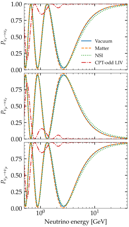
Figure 2: Two-neutrino oscillation probabilities $P_{\nu_{e}\to\nu_{e}}$ (top), $P_{\nu_{\mu}\to\nu_{e}}$ (center), and $P_{\nu_{\mu}\to\nu_{\mu}}$ (bottom), computed using the method presented here, via NuOscProbExact Bustamante . This figure is the two-neutrino counterpart of Fig. 1. See the main text and Appendix E for details.

Appendix E Sample two-neutrino Hamiltonians

Here we present the two-neutrino Hamiltonians included as examples in NuOscProbExact. These are the two-neutrino counterparts of the three-neutrino examples presented in Section VI; we refer to that section for a description of each scenario. All of the Hamiltonians below are written in the flavor basis.

Figure 2 shows the probabilities $P_{\nu_{e}\to\nu_{e}}$, $P_{\nu_{\mu}\to\nu_{e}}$, and $P_{\nu_{\mu}\to\nu_{\mu}}$ for the same four scenarios as in Fig. 1, computed using NuOscProbExact Bustamante . Again, we set the baseline to $L=1300$ km. The parameters and their values used in each example case are introduced below; they are a selection of the ones used in Fig. 1.

For oscillations in vacuum, we use Eq. (23), i.e.,

$$\mathbb{H}_{2}^{\rm vac}(E)=\frac{1}{2E}\mathbb{R}_{2,\theta}\mathbb{M}_{2}^{2}\mathbb{R}_{2,\theta}^{\dagger}\;,$$

where the rotation matrix $\mathbb{R}_{2,\theta}$ is given in Eq. (22), in terms of the mixing angle $\theta$. In Fig. 2, we set $\theta$ and $\Delta m^{2}$, respectively, to the values of $\theta_{12}$ and $\Delta m_{21}^{2}$ used in Fig. 1.

For oscillations in matter, we use

$$\mathbb{H}_{2}^{\rm matt}(E)=\mathbb{H}_{2}^{\rm vac}(E)+\mathbb{A}_{2}\;,$$

where $\mathbb{A}_{2}\equiv{\rm diag}(V_{\rm CC},0)$ and $V_{\rm CC}$ is defined as before. In Fig. 2, we set $\rho=3$ g cm^-3.

For oscillations in matter with non-standard interactions, we use González-García and Maltoni (2004); González-García et al. (2005)

$$\mathbb{H}_{2}^{\rm NSI}(E)=\mathbb{H}_{2}^{\rm vac}(E)+\mathbb{A}_{2}+\mathbb{V}_{2}\;,$$

where $\mathbb{V}_{2}\equiv V_{\rm CC}\epsilon_{2}$ and the matrix of NSI strength parameters is

$$\epsilon_{2}=\left(\begin{array}[]{ccc}\epsilon_{ee}&\epsilon_{e\mu}\\ \epsilon_{e\mu}^{\ast}&\epsilon_{\mu\mu}\\ \end{array}\right)\;.$$

In Fig. 2, we set $\epsilon_{ee}=-\epsilon_{e\mu}=0.06$ and $\epsilon_{\mu\mu}=1.2$.

For oscillations in a CPT-odd Lorentz-violating background, we use González-García and Maltoni (2004); González-García et al. (2005)

$$\mathbb{H}_{2}^{\rm LIV}(E)=\mathbb{H}_{2}^{\rm vac}(E)+\frac{E}{\Lambda}\mathbb{R}_{2,\xi}\mathbb{B}_{2}\mathbb{R}_{2,\xi}^{\dagger}\;,$$

where $\mathbb{U}_{2,\xi}$ is a $2\times 2$ rotation matrix, like Eq. (22), but evaluated at a different mixing angle $\xi$. In Fig. 2, we set $\mathbb{R}_{2,\xi}=\mathbb{1}$, $b_{1}/\Lambda=10^{-21}$, and $b_{2}/\Lambda=5\cdot 10^{-21}$.