Pion generalized parton distribution from lattice QCD

Abstract

We present the first lattice calculation of the valence-quark generalized parton distribution (GPD) of the pion using the large-momentum effective theory (LaMET) approach. We focus on the zero-skewness limit, where the GPD has a probability-density interpretation in the longitudinal Bjorken $x$ and the transverse impact-parameter distributions. Our calculation is done using clover valence fermions on an ensemble of gauge configurations with $2+1+1$ flavors (degenerate up/down, strange and charm) of highly improved staggered quarks (HISQ) with lattice spacing $a\approx 0.12$ fm, box size $L\approx 3$ fm and pion mass $m_{\pi}\approx 310$ MeV. The parton distribution function and the form factor are reproduced as special limits of the GPD as expected. Due to the large errors, this exploratory study does not show a clear preference among different model assumptions about the kinematic dependence of the GPD. To discriminate between these assumptions, future studies using higher-statistics data will be crucial.

I Introduction

In the past few decades, extensive studies of parton distribution functions (PDFs) have provided us with detailed knowledge of the longitudinal momentum distribution of quarks and gluons, and, therefore, a one-dimensional picture of hadrons. To map out the multidimensional partonic structure of hadrons, which is an important goal for experiments carried out at the existing facilities in DESY, JLab, BNL, CERN or the planned Electron-Ion Collider, we need to study quantities exhibiting the transverse structure of hadrons. One such quantity that has attracted a lot of interest in the past few years are the generalized parton distributions (GPDs) Ji (1997a, b) (see also Müller et al. (1994)).

The GPDs unify seemingly different physical quantities, such as the PDFs and hadron form factors, into the same framework. They offer a description of the correlations between the transverse position and longitudinal momentum of quarks and gluons inside the nucleon, thereby giving access to quark and gluon orbital angular momentum contributions to the nucleon spin Ji (1997a). Experimentally, the GPDs can be accessed through hard exclusive processes like deeply virtual Compton scattering or meson production. Useful constraints on the forms of the nucleon GPDs have been obtained from measurements of such processes at DESY Airapetian et al. (2001); Adloff et al. (2001); Chekanov et al. (2003) and JLab Defurne et al. (2015); Jo et al. (2015); Seder et al. (2015); Dudek et al. (2012). However, as the GPDs usually contribute to experimental observables through convolutions and they have more complicated kinematic dependence than the PDFs, extracting the GPDs from these experimental measurements is in general rather difficult. Therefore, inputs from theory are important and play a complementary role in determining the GPDs. Valuable insights are gained through computations using models (see e.g. Ref. Belitsky and Radyushkin (2005) for a review) and lattice QCD. So far, computations using the latter are limited to the first few moments of the GPDs Gockeler et al. (2004); Hagler et al. (2003); LHPC et al. (2004); Gockeler et al. (2005) (see Ref. Hagler (2010) for a review).

In recent years, a new theory framework has been developed that allows for lattice calculations of the $x$-dependence, instead of the moments, of parton quantities Ji (2013, 2014). This theory is now known as the large-momentum effective theory (LaMET). In this approach, a parton observable such as the PDFs or the GPDs can be accessed from lattice QCD in the following manner: 1) Construct an appropriate static-operator matrix element (a quasi-observable) that approaches the parton observable in the large-momentum limit of the external hadron. The quasi-observable constructed this way is usually hadron-momentum–dependent but time-independent, and, therefore, can be readily computed on the lattice. 2) Calculate the quasi-observable on the lattice. 3) Convert it to the parton observable through a factorization formula accurate up to power corrections that are suppressed by the hadron momentum. The existence of such a factorization is ensured by construction; for a proof, see Refs. Ma and Qiu (2018); Izubuchi et al. (2018); Liu et al. (2019).

Since LaMET was proposed, a lot of progress has been achieved with respect to both the theoretical understanding of the formalism Xiong et al. (2014); Ji and Zhang (2015); Ji et al. (2015a); Xiong and Zhang (2015); Ji et al. (2015b); Monahan (2018); Ji et al. (2018a); Stewart and Zhao (2018); Constantinou and Panagopoulos (2017); Green et al. (2018); Izubuchi et al. (2018); Xiong et al. (2017); Wang et al. (2018); Wang and Zhao (2018); Xu et al. (2018a); Chen et al. (2016); Zhang et al. (2017); Ishikawa et al. (2016); Chen et al. (2017a); Ji et al. (2018b); Ishikawa et al. (2017); Chen et al. (2018a); Alexandrou et al. (2017a); Constantinou and Panagopoulos (2017); Green et al. (2018); Chen et al. (2018a, 2017b); Lin et al. (2018a); Chen et al. (2017c); Li (2016); Monahan and Orginos (2017); Radyushkin (2017); Rossi and Testa (2017); Carlson and Freid (2017); Ji et al. (2017); Briceño et al. (2018); Hobbs (2018); Jia et al. (2017); Xu et al. (2018b); Jia et al. (2018); Spanoudes and Panagopoulos (2018); Rossi and Testa (2018); Liu et al. (2018a); Ji et al. (2019); Bhattacharya et al. (2019a); Radyushkin (2019); Zhang et al. (2019a); Li et al. (2019); Braun et al. (2019) and its application to lattice calculations of nucleon and meson PDFs, as well as meson distribution amplitudes Lin et al. (2015); Chen et al. (2016); Lin et al. (2018a); Alexandrou et al. (2015, 2017b, 2017a); Chen et al. (2018a); Zhang et al. (2017, 2019b); Alexandrou et al. (2018a); Chen et al. (2018b, c); Alexandrou et al. (2018b); Lin et al. (2018b); Fan et al. (2018); Liu et al. (2018b); Wang et al. (2019). Despite limited volumes and relatively coarse lattice spacings, the state-of-the-art nucleon isovector quark PDFs determined from lattice data at the physical point have shown reasonable agreement Chen et al. (2018b); Lin et al. (2018b); Alexandrou et al. (2018a) with phenomenological results extracted from the experimental data Dulat et al. (2016); Ball et al. (2017); Harland-Lang et al. (2015); Nocera et al. (2014); Ethier et al. (2017). Of course, a careful study of theoretical uncertainties and lattice artifacts is still needed to fully establish the reliability of the results.

As for the GPDs, the factorization of the isovector quark quasi-GPDs has been proven to leading-power accuracy using the operator product expansion Liu et al. (2019), and the corresponding hard matching function was also computed both in a cutoff scheme Ji et al. (2015a); Xiong and Zhang (2015) and in a regularization-independent momentum-subtraction (RI/MOM) scheme Liu et al. (2019) (for studies of quasi-GPDs in diquark models see e.g. Bhattacharya et al. (2019a, b)). This allows us to perform exploratory studies on the quark GPDs once we have lattice simulations of the corresponding quasi-GPD matrix elements.

In this paper, we carry out the first lattice calculation of the valence-quark GPD of the pion using the LaMET approach. As a first step, we focus on the zero-skewness limit, that is, the momentum transfer between the initial and final states is purely transverse. In this limit, the quark GPD is related to the impact-parameter distribution of quarks that has a probability-density interpretation Burkardt (2003) (see also Ref. Ralston and Pire (2002)). Our calculation is done using clover valence fermions on an ensemble of gauge configurations with $2+1+1$ flavors (degenerate up/down, strange and charm) of highly improved staggered quarks (HISQ) Follana et al. (2007) generated by the MILC Collaboration Bazavov et al. (2013) with lattice spacing $a\approx 0.12$ fm, box size $L\approx 3$ fm and pion mass $m_{\pi}\approx 310$ MeV.

II From quasi-GPD to GPD in the pion

The unpolarized quark GPD in the pion is defined on the lightcone as

$$H_{q}^{\pi}(x,\xi,t,\mu)=\int\frac{d\eta^{-}}{4\pi}e^{-ix\eta^{-}P^{+}}\\ \times\big{\langle}\pi(P+\frac{\Delta}{2})\left|{\bar{q}}(\frac{\eta^{-}}{2})\gamma^{+}\Gamma(\frac{\eta^{-}}{2},-\frac{\eta^{-}}{2})q(-\frac{\eta^{-}}{2})\right|\pi(P-\frac{\Delta}{2})\big{\rangle},$$ (1)

where $\bar{q},q$ denote the quark fields, $\eta^{\pm}=(\eta^{0}\pm\eta^{3})/\sqrt{2}$, and $x\in[-1,1]$. The pion momentum of the initial(final) state is $P\mp\Delta/2$ with $\Delta$ the momentum transfer and $P^{\mu}=(P^{0},0,0,P^{z})$. The variables

$$t=\Delta^{2},\hskip 20.00003pt\xi=-\frac{\Delta^{+}}{2P^{+}},$$ (2)

and $\mu$ is the renormalization scale in the $\overline{\text{MS}}$ scheme. The gauge link

$$\Gamma(\eta_{2}^{-},\eta_{1}^{-}) =\exp\bigg{(}-ig\int_{\eta_{1}^{-}}^{\eta_{2}^{-}}d\eta^{-}A^{+}(\eta^{-})\bigg{)}\,$$ (3)

ensures gauge invariance of the quark bilinear operator. Eq. (1) is an off-forward matrix element where the momenta for the initial and final states are different. In the forward ($\Delta^{\mu}\to 0$) limit, it reduces to the PDF.

An appropriate quark quasi-GPD that can be computed on the lattice is given by

$$\tilde{H}_{q}^{\pi}(x,\xi,t,P^{z},\tilde{\mu})=\int\frac{dzP^{z}}{2\pi}e^{ixP^{z}z}\tilde{h}(z,P^{z},\xi,t,\tilde{\mu})$$ (4)

with

$$\tilde{h}(z,P^{z},\xi,t,\tilde{\mu})=\\ \frac{1}{2P^{0}}\big{\langle}\pi(P+\frac{\Delta}{2})\left|\bar{q}(\frac{z}{2})\gamma^{t}\Gamma(\frac{z}{2},-\frac{z}{2})q(-\frac{z}{2})\right|\pi(P-\frac{\Delta}{2})\big{\rangle},$$ (5)

where we have chosen the Dirac matrix as $\gamma^{t}$, since it has the advantage of avoiding mixing with the scalar quark operator Constantinou and Panagopoulos (2017); Chen et al. (2017b) when a non-chiral lattice fermion is used. This choice will be used throughout this paper. The skewness parameter $\xi$ in Eq. (4) is defined as $\xi=-\Delta^{z}/(2P^{z})$, which differs from the lightcone definition in Eq. (1) by power-suppressed contributions of ${\cal O}(m_{\pi}^{2}/P_{z}^{2})$. We have ignored this difference and denoted it with the same label as the skewness in the GPD. $\tilde{\mu}$ denotes the renormalization scale in an appropriate renormalization scheme for the quasi-GPD. In the present paper, we will focus on the $u-d$ combination at zero skewness $\xi=0$, where the former avoids contributions from disconnected diagrams as well as the mixing with gluon GPDs, while the latter simplifies the kinematic dependence of the quark GPD and is also related to the impact-parameter distribution of quarks that has a probability-density interpretation Burkardt (2000, 2003).

The bare pion matrix element on the right-hand side of Eq. (4) can be calculated on the lattice. In Refs. Ji et al. (2018b); Ishikawa et al. (2017); Green et al. (2018), it has been shown that the quark bilinear operator defining $\tilde{h}$ is multiplicatively renormalized, and the renormalization factor can be calculated nonperturbatively on the lattice. In our previous study of the pion PDF Chen et al. (2018c), we chose to calculate the renormalization factor in the RI/MOM scheme, where the counterterm is determined by requiring that it cancels all the loop contributions for the matrix element in an off-shell external quark state at a specific momentum Stewart and Zhao (2018); Chen et al. (2018a). In other words, the renormalization factor in

$$\tilde{h}_{R}(z,P^{z},\xi,t,p_{z}^{R},\mu_{R})=$$

$$\hskip 40.00006ptZ^{-1}(z,p_{z}^{R},\mu_{R},a)\tilde{h}(z,P^{z},\xi,t,a)$$ (6)

is fixed by

$$Z(z,p^{R}_{z},\mu_{R},a)=\left.\frac{{\rm Tr}[\Lambda_{\gamma^{t}}\cal P]}{{\rm Tr}[\Lambda_{\gamma^{t}}\cal P]_{\rm tree}}\right|_{\tiny\begin{matrix}p^{2}=-\mu_{R}^{2}\\ \!\!\!\!p_{z}=p^{R}_{z}\end{matrix}},$$ (7)

where $\Lambda_{\gamma^{t}}$ is the amputated Green function of the forward quark bilinear operator in Eq. (5) in an off-shell quark state with momentum $p$. $\cal P$ is a projection operator that defines the RI/MOM renormalization factor, $\mu_{R},p_{z}^{R}$ are renormalization scales introduced in the RI/MOM scheme. After renormalization, all singular dependence on $a$ has been removed, and $\tilde{h}_{R}$ has a well-defined continuum limit. We have suppressed the residual $a$ dependence in $\tilde{h}_{R}$. The $Z$ factor defined in Eq. (7) coincides with that of the quark quasi-PDF. Since the UV divergence of the above hadron matrix element depends only on the operator defining it and not on the external state, the same renormalization factor can be used to renormalize the quark quasi-GPD matrix element. After renormalization, ${\tilde{h}}_{R}(z,P^{z},\xi,t,p_{z}^{R},\mu_{R})$ can be converted to $\tilde{H}_{q}^{\pi}$ through a Fourier transform

$$\tilde{H}_{u-d,R}^{\pi}(x,\xi,t,P^{z},p_{z}^{R},\mu_{R}) =$$

$$\int\frac{dzP^{z}}{2\pi}e^{ixP^{z}z}{\tilde{h}}_{R}(z,P^{z},\xi,t,p_{z}^{R},\mu_{R}),$$ (8)

which can then be factorized into the normal GPD in the $\overline{\text{MS}}$ scheme convoluted with a perturbative hard matching kernel, up to power corrections that are suppressed by the pion momentum Liu et al. (2019)

$$\tilde{H}_{u-d,R}^{\pi}(x,\xi,t,P^{z},p_{z}^{R},\mu_{R})$$

$$= \int_{-1}^{1}{dy\over|y|}C\left({x\over y},\frac{\xi}{y},\frac{\mu_{R}}{p_{z}^{R}},\frac{yP^{z}}{\mu},\frac{yP^{z}}{p_{z}^{R}}\right)H_{u-d}^{\pi}(y,\xi,t,\mu)$$

$$+ \mathcal{O}\left({\tilde{m}_{\pi}^{2}\over P_{z}^{2}},{\Lambda_{\text{QCD}}^{2}\over{P_{z}^{2}}}\right),$$ (9)

where $\mu$ is the renormalization scale of the GPD. The matching kernel $C$ has been worked out at one-loop in Ref. Liu et al. (2019). At zero skewness $\xi=0$, $C$ is the same as the matching kernel for the PDF that is documented in Refs. Chen et al. (2018b); Liu et al. (2018a). Ideally, the continuum limit of $\tilde{H}_{u-d,R}$ should be taken before applying the matching so that lattice artifacts can be removed and the rotational symmetry recovered. However, only a single lattice spacing is used in the present work. The continuum limit can be explored in the future once we have more data at different lattice spacings.

For the power corrections, the meson-mass correction associated with the choice of Dirac matrix $\gamma^{t}$ is identical to that of the helicity distribution worked out in Ref. Chen et al. (2016) with the replacement $m_{\pi}^{2}\to\tilde{m}_{\pi}^{2}=m_{\pi}^{2}-t/4$. The $\mathcal{O}({\Lambda_{\text{QCD}}^{2}/P_{z}^{2}})$ correction is parametrically about the same size as the $\mathcal{O}({\tilde{m}_{\pi}^{2}/P_{z}^{2}})$ correction (except for very small or large $x$ where the correction behaves like $\mathcal{O}({\Lambda_{\text{QCD}}^{2}/(x^{2}(1-x)P_{z}^{2})})$ due to renormalon ambiguity, as argued in Ref. Braun et al. (2019)), and is negligible compared with other sources of errors.

For $\tilde{H}_{u-d}^{\pi^{+}}$, the matrix element $\tilde{h}$ is purely real in the isospin symmetric limit which is adopted in this work. This is because the imaginary part of the matrix element is related to the inverse Fourier transform of $\tilde{H}_{u-d}^{\pi^{+}}(x)-\tilde{H}_{u-d}^{\pi^{+}}(-x)$, which is $\tilde{H}_{u-d}^{\pi^{+}}(x)+\tilde{H}_{\bar{u}-\bar{d}}^{\pi^{+}}(x)=0$ after applying the definition of anti-quark distribution $\tilde{H}_{\bar{q}}(|x|)=-\tilde{H}_{q}(-|x|)$ and the isospin symmetry relation $\tilde{H}^{\pi^{+}}_{u(d)}=\tilde{H}^{\pi^{+}}_{\bar{d}(\bar{u})}$. Analogously, the real part of the matrix element is related to the inverse Fourier transform of $\tilde{H}_{u-d}^{\pi^{+}}(x)+\tilde{H}_{u-d}^{\pi^{+}}(-x)=\tilde{H}_{u-d}^{\pi^{+}}(|x|)-\tilde{H}_{\bar{u}-\bar{d}}^{\pi^{+}}(|x|)$, which is the isovector quasi-GPD of the valence quark ($q_{v}\equiv q-\bar{q}$): $\tilde{H}_{u_{v}-d_{v}}^{\pi^{+}}(|x|)$.

The above analysis applies not only to the pion quasi-GPD but also to the pion GPD. In the following, we will present our skewless isovector combination of valence quark GPD for the charged pion $\pi^{+}$ as

$$H_{v}^{\pi}(x,t)\equiv\frac{1}{2}H_{u_{v}-d_{v}}^{\pi^{+}}(x,t)=H_{u_{v}}^{\pi^{+}}(x,t)=-H_{d_{v}}^{\pi^{+}}(x,t),$$ (10)

where the dependence on the renormalization scale $\mu$ is suppressed.

III Lattice calculation setup

In this work, we use a single ensemble of gauge configurations with $2+1+1$ flavors (degenerate up/down, strange and charm) of highly improved staggered quarks (HISQ) Follana et al. (2007) generated by the MILC Collaboration Bazavov et al. (2013) with lattice spacing $a\approx 0.12$ fm, pion mass $m_{\pi}\approx 310$ MeV, and box size $L\approx 3$ fm ($M_{\pi}L\approx$ 4.5). Our calculation is done using clover valence fermions on top of one-step hypercubic(HYP)-smeared Hasenfratz and Knechtli (2001) gauge links, with the clover parameters tuned to recover the lowest pion mass of the staggered quarks in the sea Gupta et al. (2017); Bhattacharya et al. (2015a, b, 2014). Then we calculate the time-independent, nonlocal (in space, chosen to be in the $z$ direction) correlators of a pion with a finite-$P^{z}$ boost

$$\tilde{h}_{\text{lat}}(z,P^{z},t,a)$$ (11)

$$= \frac{1}{2P^{0}}\left\langle\pi^{+}(\vec{P}+\frac{\vec{\Delta}}{2})\right|\bar{q}(z)\Gamma\left(\prod_{n}U_{z}(n\hat{z})\right)\tau_{3}q(0)\left|\pi^{+}(\vec{P}-\frac{\vec{\Delta}}{2})\right\rangle,$$

where $U_{z}$ is a discrete gauge link in the $z$ direction, $\vec{P}=\{0,0,P^{z}\}$ is the momentum of the pion, $\Gamma=\gamma^{t}$ and $\vec{\Delta}$ is the momentum transfer between initial and final pion. In this work, we only deal with the zero-skewness limit $\xi=0$, where the matching coincides with that for the PDF. We use 3 boosted pion momenta, $P^{z}=\{0,0,n\frac{2\pi}{L}\}$ with $n\in\{2,3,4\}$, which correspond to 0.86, 1.32 and 1.74 GeV, respectively. The initial and final pion momenta are obtained from $\{0,0,n\frac{2\pi}{L}\}\mp\vec{\Delta}/2$, where $\vec{\Delta}=\{n_{x},n_{y},0\}\frac{2\pi}{L}$ with $n_{x}^{2}+n_{y}^{2}\leq 5$ fand $P_{0}=\sqrt{(P^{z})^{2}-t/4+m_{\pi}^{2}}$. We carefully tune the Gaussian smearing parameter to best control the excited state and use four source-sink separations, 0.72, 0.84, 0.96 and 1.08 fm to help us remove excited-state contamination from our three-point correlators fits to extract the pion matrix element. We use 1840 configurations with total measurements of 29440, 29440, 58880 and 58880 from the smallest source-sink separation to largest one. After we obtain the pion form factors at each momentum, we momentum-average the spatial symmetry in the $x-y$ plane for each momentum transfer $t$.

To make sure that we have full control of excited-state contamination, we analyze our data using different source-sink separations and using different levels of excited-state treatment. First, we use the “two-sim” analysis described in Ref. Bhattacharya et al. (2014) to obtain the ground-state pion matrix elements using all 4 source-sink separations. The “two-sim” analysis only takes account of the leading excited-state contamination coming from the excited- and ground-state mixing. This is the same level as other commonly used methods, such as the “summation” method Capitani et al. (2012). A second extraction uses only the largest two separations; if there is a significant excited-state contamination at the smaller source-sink separation, 0.72 and 0.84 fm, we should see inconsistency in the ground-state matrix element between this analysis and earlier ones. Finally, we use the “two-twoRR” analysis (see Ref. Bhattacharya et al. (2014) for details), which includes an additional matrix element related to excited states. Given the same input source-sink separations for the three-point correlators, the extracted ground-state matrix elements should be noisier, since more fit parameters are used. All the above analyses generate consistent ground-state nucleon matrix elements. A few example fit plots from a subset of data are shown in Fig. 1. In the GPD analysis to be presented below, we use matrix elements from the “two-twoRR” analysis.

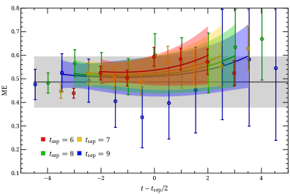
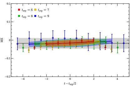
Figure 1: Example three-point ratio plots as functions of the operator insertion time $t$ from the real pion matrix elements for $z=-3$ with momentum transfer of $\{2,1,0\}\times(2\pi/L)$ (top) and for $z=6$ with momentum transfer of $\{1,0,0\}\times(2\pi/L)$ (bottom). The red, yellow, green, and blue bands are the reconstructed ratios from the fits to source-sink separation $t_{\text{sep}}=6,7,8,9$, respectively, and the gray band shows the ground-state matrix elements from the “two-simRR” fits.

Fig. 2 shows the real part of the bare and RI/MOM renormalized matrix elements for $P^{z}\in\{4\pi/L,8\pi/L\}\approx\{0.87,1.74\}$ GeV, and $t\in\{0,-2,-5\}\times(2\pi/L)^{2}$. The renormalization scales in the RI/MOM parameters have been chosen as $\mu_{R}=3.7$ GeV, $p_{z}^{R}=6\times 2\pi/L$. The error bars include statistical errors and the errors from the excited-state contamination. Systematic errors from renormalization scale dependence associated with one-loop matching, lattice spacing, non-physical pion mass and so on are not included in this figure. For $z=0$, the error at $t=0$ is much smaller than $t\neq 0$, due to charge conservation. The matrix elements at $z=0$, which are not changed by the renormalization, are the values of the pion isovector form factor. It is decreasing in $|t|$ as expected. Our form factor also agrees with the previous result (shown as points at $z=0$ in Fig. 2) obtained in Ref. Brömmel et al. (2007), which were determined from a fitted form to lattice data with a wide range of pion masses and lattice spacings and setting the pion mass to the same value used here. The errors were estimated from the difference between two fitting forms used in Ref. Brömmel et al. (2007). The error of our matrix elements at $z=0$ is larger than that in the form factor calculation, mainly because the latter is equivalent to having $P^{z}=0$ while we need nonzero $P^{z}$ to access the full distribution.

IV Numerical results and discussion

Now we present our numerical results for the valence quark GPD in the pion. As mentioned previously, the bare quasi-GPD matrix element calculated on the lattice can be renormalized by the RI/MOM renormalization factors for the quasi-PDF matrix element, which have been computed in Ref. Liu et al. (2018a). The momentum distribution is then given by

$$\tilde{H}_{v}^{\pi}(x)=\int\frac{dz}{4\pi}e^{ixzP^{z}}\tilde{h}_{\text{lat},R}(z),$$ (12)

where only the $z$ and $x$ dependence is shown for simplicity. Following our earlier work Lin et al. (2018a) on the nucleon PDF, we also apply the “derivative” method Lin et al. (2018a) to improve the truncation error in the Fourier transform in Eq. (12). We then apply the one-loop matching and meson-mass corrections, where the latter turn out to be numerically negligible.

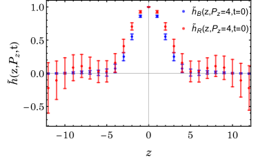
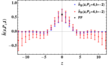
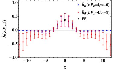
Figure 2: The real part of the bare and renormalized matrix elements, ${\tilde{h}}_{B}(z,P^{z},t)$ and ${\tilde{h}}_{R}(z,P^{z},t)$, for the zero-skewness isovector valence quark GPD of the pion. The averaged pion momentum in the $z$-direction is $P^{z}=4$ (left to right, in units of $(2\pi/L)$) and the momentum transfer squared is $t=\{0,-2,-5\}$ (top to bottom, in units of $(2\pi/L)^{2}$). Also plotted at $z=0$ are the form factors (FF) from previous lattice calculations Brömmel et al. (2007) at the same pion mass.

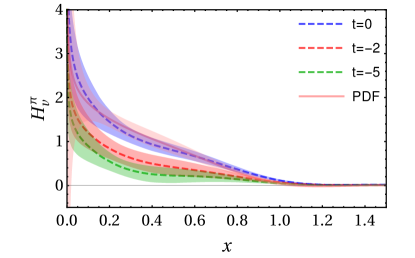
Figure 3: The zero-skewness pion valence quark GPD $H^{\pi^{+}}_{v}(x,\xi=0,t,\mu=4\text{GeV})$ for $t=\{0,-2,-5\}(2\pi/L)^{2}$ after one-loop matching and the meson-mass correction. “PDF” denotes the pion PDF result in Ref. Chen et al. (2018c).

In Fig. 3, we show the results of the valence-quark distribution $H_{v}^{\pi}(x,t,\mu)$ for different values of $t$ with the renormalization scale $\mu=4$ GeV. We have inverted the factorization formula in Eq. (II) by perturbatively expanding the matching kernel $C$ to ${\cal O}(\alpha_{s})$. Also, the meson-mass power corrections have been removed. For the RI/MOM renormalization of the quark quasi-GPD, we have chosen $\mu_{R}=3.7$ GeV, $p_{z}^{R}=6\times 2\pi/L$. The error bands in Fig. 3 include statistical as well as systematic errors of $p_{z}^{R}$ dependence by varying it between $4\times 2\pi/L$ and $8\times 2\pi/L$. The curve with $t=0$ is consistent with our previous result Chen et al. (2018c) within errors. As a consistency check, we also tested that the $x$-integral of the GPDs in Fig. 3 reproduces the form factors in Fig. 2 within 1 standard deviation. The impact parameter-space distribution can in principle be obtained by Fourier transforming the $t$ dependence to the impact parameter $b_{\perp}$ dependence. However, we have only the results for very few values of $t$ in this work.

For the kinematic dependence of $H_{v}^{\pi}(x,t,\mu)$, a naive functional form is

$$H_{v}^{\pi}(x,t,\mu)=q_{v}^{\pi}(x,\mu)F_{u-d}^{\pi}(t),$$ (13)

where $q^{\pi}_{v}$ is the pion valence-quark PDF satisfying $\int dx\,q^{\pi}_{v}(x,\mu)=1$, and $F^{\pi}_{u-d}(t)$ is the isovector form factor of $\pi^{+}$ with the normalization $F^{\pi}_{u-d}(0)=1$. This parametrization is simple, but not favored by the study of the GPD asymptotic behavior at $x\to 1$ Burkardt (2003); Diehl et al. (2005). On the lattice side, Eq.(13) implies factorization of the bare matrix element

$$\tilde{h}_{\text{lat}}(z,P^{z},t,a)=F^{\pi}_{u-d}(t)\tilde{h}_{\text{lat}}(z,P^{z},t\emph{}=0,a),$$ (14)

which makes it easier to be checked with lattice QCD.

Another useful parametrization is

$$H_{v}^{\pi}(x,t,\mu)=q_{v}^{\pi}(x,\mu)\exp[tf_{q}(x,\mu)],$$ (15)

with $f_{q}$ an unknown function. This parametrization has been used to fit the unpolarized zero-skewness GPD of the nucleon and in discussing the fit to experimental data for the nucleon form factors Diehl et al. (2005).

With current uncertainties, our results are consistent with both parametrizations. Future high-statistics studies will be able to provide guidance to the kinematic dependence of the GPDs, and in particular allow differentiation between various models that are commonly used.

V Summary

We have presented the first lattice calculation of the valence-quark generalized parton distribution of the pion using the LaMET approach. We have focused on the zero-skewness limit, where the GPD has a probability-density interpretation in the longitudinal Bjorken $x$ and the transverse impact-parameter distributions. Our calculation is done using clover valence fermions on an ensemble of gauge configurations with $2+1+1$ flavors (degenerate up/down, strange and charm) of highly improved staggered quarks (HISQ) with lattice spacing $a\approx 0.12$ fm, box size $L\approx 3$ fm and pion mass $m_{\pi}\approx 310$ MeV. The parton distribution function and form factor are reproduced as special limits of the GPD as expected. Future studies using higher-statistics data will be crucial to provide guidance to the kinematic dependence of the GPDs and to differentiate models that are commonly used.

References

- Ji (1997a) X.-D. Ji, Phys. Rev. Lett. 78, 610 (1997a), arXiv:hep-ph/9603249 [hep-ph] .
- Ji (1997b) X.-D. Ji, Phys. Rev. D55, 7114 (1997b), arXiv:hep-ph/9609381 [hep-ph] .
- Müller et al. (1994) D. Müller, D. Robaschik, B. Geyer, F. M. Dittes, and J. Hořejši, Fortsch. Phys. 42, 101 (1994), arXiv:hep-ph/9812448 [hep-ph] .
- Airapetian et al. (2001) A. Airapetian et al. (HERMES), Phys. Rev. Lett. 87, 182001 (2001), arXiv:hep-ex/0106068 [hep-ex] .
- Adloff et al. (2001) C. Adloff et al. (H1), Phys. Lett. B517, 47 (2001), arXiv:hep-ex/0107005 [hep-ex] .
- Chekanov et al. (2003) S. Chekanov et al. (ZEUS), Phys. Lett. B573, 46 (2003), arXiv:hep-ex/0305028 [hep-ex] .
- Defurne et al. (2015) M. Defurne et al. (Jefferson Lab Hall A), Phys. Rev. C92, 055202 (2015), arXiv:1504.05453 [nucl-ex] .
- Jo et al. (2015) H. S. Jo et al. (CLAS), Phys. Rev. Lett. 115, 212003 (2015), arXiv:1504.02009 [hep-ex] .
- Seder et al. (2015) E. Seder et al. (CLAS), Phys. Rev. Lett. 114, 032001 (2015), [Addendum: Phys. Rev. Lett.114,no.8,089901(2015)], arXiv:1410.6615 [hep-ex] .
- Dudek et al. (2012) J. Dudek et al., Eur. Phys. J. A48, 187 (2012), arXiv:1208.1244 [hep-ex] .
- Belitsky and Radyushkin (2005) A. V. Belitsky and A. V. Radyushkin, Phys. Rept. 418, 1 (2005), arXiv:hep-ph/0504030 [hep-ph] .
- Gockeler et al. (2004) M. Gockeler, R. Horsley, D. Pleiter, P. E. L. Rakow, A. Schafer, G. Schierholz, and W. Schroers (QCDSF), Phys. Rev. Lett. 92, 042002 (2004), arXiv:hep-ph/0304249 [hep-ph] .
- Hagler et al. (2003) P. Hagler, J. W. Negele, D. B. Renner, W. Schroers, T. Lippert, and K. Schilling (LHPC, SESAM), Phys. Rev. D68, 034505 (2003), arXiv:hep-lat/0304018 [hep-lat] .
- LHPC et al. (2004) LHPC, P. Hagler, J. W. Negele, D. B. Renner, W. Schroers, T. Lippert, and K. Schilling (LHPC, SESAM), Phys. Rev. Lett. 93, 112001 (2004), arXiv:hep-lat/0312014 [hep-lat] .
- Gockeler et al. (2005) M. Gockeler, P. Hagler, R. Horsley, D. Pleiter, P. E. L. Rakow, A. Schafer, G. Schierholz, and J. M. Zanotti (QCDSF, UKQCD), Phys. Lett. B627, 113 (2005), arXiv:hep-lat/0507001 [hep-lat] .
- Hagler (2010) P. Hagler, Phys. Rept. 490, 49 (2010), arXiv:0912.5483 [hep-lat] .
- Ji (2013) X. Ji, Phys. Rev. Lett. 110, 262002 (2013), arXiv:1305.1539 [hep-ph] .
- Ji (2014) X. Ji, Sci. China Phys. Mech. Astron. 57, 1407 (2014), arXiv:1404.6680 [hep-ph] .
- Ma and Qiu (2018) Y.-Q. Ma and J.-W. Qiu, Phys. Rev. Lett. 120, 022003 (2018), arXiv:1709.03018 [hep-ph] .
- Izubuchi et al. (2018) T. Izubuchi, X. Ji, L. Jin, I. W. Stewart, and Y. Zhao, Phys. Rev. D98, 056004 (2018), arXiv:1801.03917 [hep-ph] .
- Liu et al. (2019) Y.-S. Liu, W. Wang, J. Xu, Q.-A. Zhang, J.-H. Zhang, S. Zhao, and Y. Zhao, (2019), arXiv:1902.00307 [hep-ph] .
- Xiong et al. (2014) X. Xiong, X. Ji, J.-H. Zhang, and Y. Zhao, Phys. Rev. D90, 014051 (2014), arXiv:1310.7471 [hep-ph] .
- Ji and Zhang (2015) X. Ji and J.-H. Zhang, Phys. Rev. D92, 034006 (2015), arXiv:1505.07699 [hep-ph] .
- Ji et al. (2015a) X. Ji, A. Schäfer, X. Xiong, and J.-H. Zhang, Phys. Rev. D92, 014039 (2015a), arXiv:1506.00248 [hep-ph] .
- Xiong and Zhang (2015) X. Xiong and J.-H. Zhang, Phys. Rev. D92, 054037 (2015), arXiv:1509.08016 [hep-ph] .
- Ji et al. (2015b) X. Ji, P. Sun, X. Xiong, and F. Yuan, Phys. Rev. D91, 074009 (2015b), arXiv:1405.7640 [hep-ph] .
- Monahan (2018) C. Monahan, Phys. Rev. D97, 054507 (2018), arXiv:1710.04607 [hep-lat] .
- Ji et al. (2018a) X. Ji, L.-C. Jin, F. Yuan, J.-H. Zhang, and Y. Zhao, (2018a), arXiv:1801.05930 [hep-ph] .
- Stewart and Zhao (2018) I. W. Stewart and Y. Zhao, Phys. Rev. D97, 054512 (2018), arXiv:1709.04933 [hep-ph] .
- Constantinou and Panagopoulos (2017) M. Constantinou and H. Panagopoulos, Phys. Rev. D96, 054506 (2017), arXiv:1705.11193 [hep-lat] .
- Green et al. (2018) J. Green, K. Jansen, and F. Steffens, Phys. Rev. Lett. 121, 022004 (2018), arXiv:1707.07152 [hep-lat] .
- Xiong et al. (2017) X. Xiong, T. Luu, and U.-G. Meißner, (2017), arXiv:1705.00246 [hep-ph] .
- Wang et al. (2018) W. Wang, S. Zhao, and R. Zhu, Eur. Phys. J. C78, 147 (2018), arXiv:1708.02458 [hep-ph] .
- Wang and Zhao (2018) W. Wang and S. Zhao, JHEP 05, 142 (2018), arXiv:1712.09247 [hep-ph] .
- Xu et al. (2018a) J. Xu, Q.-A. Zhang, and S. Zhao, Phys. Rev. D97, 114026 (2018a), arXiv:1804.01042 [hep-ph] .
- Chen et al. (2016) J.-W. Chen, S. D. Cohen, X. Ji, H.-W. Lin, and J.-H. Zhang, Nucl. Phys. B911, 246 (2016), arXiv:1603.06664 [hep-ph] .
- Zhang et al. (2017) J.-H. Zhang, J.-W. Chen, X. Ji, L. Jin, and H.-W. Lin, Phys. Rev. D95, 094514 (2017), arXiv:1702.00008 [hep-lat] .
- Ishikawa et al. (2016) T. Ishikawa, Y.-Q. Ma, J.-W. Qiu, and S. Yoshida, (2016), arXiv:1609.02018 [hep-lat] .
- Chen et al. (2017a) J.-W. Chen, X. Ji, and J.-H. Zhang, Nucl. Phys. B915, 1 (2017a), arXiv:1609.08102 [hep-ph] .
- Ji et al. (2018b) X. Ji, J.-H. Zhang, and Y. Zhao, Phys. Rev. Lett. 120, 112001 (2018b), arXiv:1706.08962 [hep-ph] .
- Ishikawa et al. (2017) T. Ishikawa, Y.-Q. Ma, J.-W. Qiu, and S. Yoshida, Phys. Rev. D96, 094019 (2017), arXiv:1707.03107 [hep-ph] .
- Chen et al. (2018a) J.-W. Chen, T. Ishikawa, L. Jin, H.-W. Lin, Y.-B. Yang, J.-H. Zhang, and Y. Zhao, Phys. Rev. D97, 014505 (2018a), arXiv:1706.01295 [hep-lat] .
- Alexandrou et al. (2017a) C. Alexandrou, K. Cichy, M. Constantinou, K. Hadjiyiannakou, K. Jansen, H. Panagopoulos, and F. Steffens, Nucl. Phys. B923, 394 (2017a), arXiv:1706.00265 [hep-lat] .
- Chen et al. (2017b) J.-W. Chen, T. Ishikawa, L. Jin, H.-W. Lin, Y.-B. Yang, J.-H. Zhang, and Y. Zhao, (2017b), arXiv:1710.01089 [hep-lat] .
- Lin et al. (2018a) H.-W. Lin, J.-W. Chen, T. Ishikawa, and J.-H. Zhang (LP3), Phys. Rev. D98, 054504 (2018a), arXiv:1708.05301 [hep-lat] .
- Chen et al. (2017c) J.-W. Chen, T. Ishikawa, L. Jin, H.-W. Lin, A. Schäfer, Y.-B. Yang, J.-H. Zhang, and Y. Zhao, (2017c), arXiv:1711.07858 [hep-ph] .
- Li (2016) H.-n. Li, Phys. Rev. D94, 074036 (2016), arXiv:1602.07575 [hep-ph] .
- Monahan and Orginos (2017) C. Monahan and K. Orginos, JHEP 03, 116 (2017), arXiv:1612.01584 [hep-lat] .
- Radyushkin (2017) A. Radyushkin, Phys. Lett. B767, 314 (2017), arXiv:1612.05170 [hep-ph] .
- Rossi and Testa (2017) G. C. Rossi and M. Testa, Phys. Rev. D96, 014507 (2017), arXiv:1706.04428 [hep-lat] .
- Carlson and Freid (2017) C. E. Carlson and M. Freid, Phys. Rev. D95, 094504 (2017), arXiv:1702.05775 [hep-ph] .
- Ji et al. (2017) X. Ji, J.-H. Zhang, and Y. Zhao, Nucl. Phys. B924, 366 (2017), arXiv:1706.07416 [hep-ph] .
- Briceño et al. (2018) R. A. Briceño, J. V. Guerrero, M. T. Hansen, and C. J. Monahan, Phys. Rev. D98, 014511 (2018), arXiv:1805.01034 [hep-lat] .
- Hobbs (2018) T. J. Hobbs, Phys. Rev. D97, 054028 (2018), arXiv:1708.05463 [hep-ph] .
- Jia et al. (2017) Y. Jia, S. Liang, L. Li, and X. Xiong, JHEP 11, 151 (2017), arXiv:1708.09379 [hep-ph] .
- Xu et al. (2018b) S.-S. Xu, L. Chang, C. D. Roberts, and H.-S. Zong, Phys. Rev. D97, 094014 (2018b), arXiv:1802.09552 [nucl-th] .
- Jia et al. (2018) Y. Jia, S. Liang, X. Xiong, and R. Yu, Phys. Rev. D98, 054011 (2018), arXiv:1804.04644 [hep-th] .
- Spanoudes and Panagopoulos (2018) G. Spanoudes and H. Panagopoulos, Phys. Rev. D98, 014509 (2018), arXiv:1805.01164 [hep-lat] .
- Rossi and Testa (2018) G. Rossi and M. Testa, Phys. Rev. D98, 054028 (2018), arXiv:1806.00808 [hep-lat] .
- Liu et al. (2018a) Y.-S. Liu, J.-W. Chen, L. Jin, H.-W. Lin, Y.-B. Yang, J.-H. Zhang, and Y. Zhao, (2018a), arXiv:1807.06566 [hep-lat] .
- Ji et al. (2019) X. Ji, Y. Liu, and I. Zahed, Phys. Rev. D99, 054008 (2019), arXiv:1807.07528 [hep-ph] .
- Bhattacharya et al. (2019a) S. Bhattacharya, C. Cocuzza, and A. Metz, Phys. Lett. B788, 453 (2019a), arXiv:1808.01437 [hep-ph] .
- Radyushkin (2019) A. V. Radyushkin, Phys. Lett. B788, 380 (2019), arXiv:1807.07509 [hep-ph] .
- Zhang et al. (2019a) J.-H. Zhang, X. Ji, A. Schäfer, W. Wang, and S. Zhao, Phys. Rev. Lett. 122, 142001 (2019a), arXiv:1808.10824 [hep-ph] .
- Li et al. (2019) Z.-Y. Li, Y.-Q. Ma, and J.-W. Qiu, Phys. Rev. Lett. 122, 062002 (2019), arXiv:1809.01836 [hep-ph] .
- Braun et al. (2019) V. M. Braun, A. Vladimirov, and J.-H. Zhang, Phys. Rev. D99, 014013 (2019), arXiv:1810.00048 [hep-ph] .
- Lin et al. (2015) H.-W. Lin, J.-W. Chen, S. D. Cohen, and X. Ji, Phys. Rev. D91, 054510 (2015), arXiv:1402.1462 [hep-ph] .
- Alexandrou et al. (2015) C. Alexandrou, K. Cichy, V. Drach, E. Garcia-Ramos, K. Hadjiyiannakou, K. Jansen, F. Steffens, and C. Wiese, Phys. Rev. D92, 014502 (2015), arXiv:1504.07455 [hep-lat] .
- Alexandrou et al. (2017b) C. Alexandrou, K. Cichy, M. Constantinou, K. Hadjiyiannakou, K. Jansen, F. Steffens, and C. Wiese, Phys. Rev. D96, 014513 (2017b), arXiv:1610.03689 [hep-lat] .
- Zhang et al. (2019b) J.-H. Zhang, L. Jin, H.-W. Lin, A. Schäfer, P. Sun, Y.-B. Yang, R. Zhang, Y. Zhao, and J.-W. Chen (LP3), Nucl. Phys. B939, 429 (2019b), arXiv:1712.10025 [hep-ph] .
- Alexandrou et al. (2018a) C. Alexandrou, K. Cichy, M. Constantinou, K. Jansen, A. Scapellato, and F. Steffens, Phys. Rev. Lett. 121, 112001 (2018a), arXiv:1803.02685 [hep-lat] .
- Chen et al. (2018b) J.-W. Chen, L. Jin, H.-W. Lin, Y.-S. Liu, Y.-B. Yang, J.-H. Zhang, and Y. Zhao, (2018b), arXiv:1803.04393 [hep-lat] .
- Chen et al. (2018c) J.-W. Chen, L. Jin, H.-W. Lin, Y.-S. Liu, A. Schäfer, Y.-B. Yang, J.-H. Zhang, and Y. Zhao, (2018c), arXiv:1804.01483 [hep-lat] .
- Alexandrou et al. (2018b) C. Alexandrou, K. Cichy, M. Constantinou, K. Jansen, A. Scapellato, and F. Steffens, Phys. Rev. D98, 091503 (2018b), arXiv:1807.00232 [hep-lat] .
- Lin et al. (2018b) H.-W. Lin, J.-W. Chen, X. Ji, L. Jin, R. Li, Y.-S. Liu, Y.-B. Yang, J.-H. Zhang, and Y. Zhao, Phys. Rev. Lett. 121, 242003 (2018b), arXiv:1807.07431 [hep-lat] .
- Fan et al. (2018) Z.-Y. Fan, Y.-B. Yang, A. Anthony, H.-W. Lin, and K.-F. Liu, Phys. Rev. Lett. 121, 242001 (2018), arXiv:1808.02077 [hep-lat] .
- Liu et al. (2018b) Y.-S. Liu, J.-W. Chen, L. Jin, R. Li, H.-W. Lin, Y.-B. Yang, J.-H. Zhang, and Y. Zhao, (2018b), arXiv:1810.05043 [hep-lat] .
- Wang et al. (2019) W. Wang, J.-H. Zhang, S. Zhao, and R. Zhu, (2019), arXiv:1904.00978 [hep-ph] .
- Dulat et al. (2016) S. Dulat, T.-J. Hou, J. Gao, M. Guzzi, J. Huston, P. Nadolsky, J. Pumplin, C. Schmidt, D. Stump, and C. P. Yuan, Phys. Rev. D93, 033006 (2016), arXiv:1506.07443 [hep-ph] .
- Ball et al. (2017) R. D. Ball et al. (NNPDF), Eur. Phys. J. C77, 663 (2017), arXiv:1706.00428 [hep-ph] .
- Harland-Lang et al. (2015) L. A. Harland-Lang, A. D. Martin, P. Motylinski, and R. S. Thorne, Eur. Phys. J. C75, 204 (2015), arXiv:1412.3989 [hep-ph] .
- Nocera et al. (2014) E. R. Nocera, R. D. Ball, S. Forte, G. Ridolfi, and J. Rojo (NNPDF), Nucl. Phys. B887, 276 (2014), arXiv:1406.5539 [hep-ph] .
- Ethier et al. (2017) J. J. Ethier, N. Sato, and W. Melnitchouk, Phys. Rev. Lett. 119, 132001 (2017), arXiv:1705.05889 [hep-ph] .
- Bhattacharya et al. (2019b) S. Bhattacharya, C. Cocuzza, and A. Metz, (2019b), arXiv:1903.05721 [hep-ph] .
- Burkardt (2003) M. Burkardt, Int. J. Mod. Phys. A18, 173 (2003), arXiv:hep-ph/0207047 [hep-ph] .
- Ralston and Pire (2002) J. P. Ralston and B. Pire, Phys. Rev. D66, 111501 (2002), arXiv:hep-ph/0110075 [hep-ph] .
- Follana et al. (2007) E. Follana, Q. Mason, C. Davies, K. Hornbostel, G. P. Lepage, J. Shigemitsu, H. Trottier, and K. Wong (HPQCD, UKQCD), Phys. Rev. D75, 054502 (2007), arXiv:hep-lat/0610092 [hep-lat] .
- Bazavov et al. (2013) A. Bazavov et al. (MILC), Phys. Rev. D87, 054505 (2013), arXiv:1212.4768 [hep-lat] .
- Burkardt (2000) M. Burkardt, Phys. Rev. D62, 071503 (2000), [Erratum: Phys. Rev.D66,119903(2002)], arXiv:hep-ph/0005108 [hep-ph] .
- Hasenfratz and Knechtli (2001) A. Hasenfratz and F. Knechtli, Phys. Rev. D64, 034504 (2001), arXiv:hep-lat/0103029 [hep-lat] .
- Gupta et al. (2017) R. Gupta, Y.-C. Jang, H.-W. Lin, B. Yoon, and T. Bhattacharya, Phys. Rev. D96, 114503 (2017), arXiv:1705.06834 [hep-lat] .
- Bhattacharya et al. (2015a) T. Bhattacharya, V. Cirigliano, S. Cohen, R. Gupta, A. Joseph, H.-W. Lin, and B. Yoon (PNDME), Phys. Rev. D92, 094511 (2015a), arXiv:1506.06411 [hep-lat] .
- Bhattacharya et al. (2015b) T. Bhattacharya, V. Cirigliano, R. Gupta, H.-W. Lin, and B. Yoon, Phys. Rev. Lett. 115, 212002 (2015b), arXiv:1506.04196 [hep-lat] .
- Bhattacharya et al. (2014) T. Bhattacharya, S. D. Cohen, R. Gupta, A. Joseph, H.-W. Lin, and B. Yoon, Phys. Rev. D89, 094502 (2014), arXiv:1306.5435 [hep-lat] .
- Capitani et al. (2012) S. Capitani, M. Della Morte, G. von Hippel, B. Jager, A. Juttner, B. Knippschild, H. B. Meyer, and H. Wittig, Phys. Rev. D86, 074502 (2012), arXiv:1205.0180 [hep-lat] .
- Brömmel et al. (2007) D. Brömmel et al. (QCDSF/UKQCD), Eur. Phys. J. C51, 335 (2007), arXiv:hep-lat/0608021 [hep-lat] .
- Diehl et al. (2005) M. Diehl, T. Feldmann, R. Jakob, and P. Kroll, Eur. Phys. J. C39, 1 (2005), arXiv:hep-ph/0408173 [hep-ph] .
- Edwards and Joo (2005) R. G. Edwards and B. Joo (SciDAC, LHPC, UKQCD), Lattice field theory. Proceedings, 22nd International Symposium, Lattice 2004, Batavia, USA, June 21-26, 2004, Nucl. Phys. Proc. Suppl. 140, 832 (2005), [,832(2004)], arXiv:hep-lat/0409003 [hep-lat] .