Quantum noise in the spin transfer torque effect

Abstract

Describing the microscopic details of the interaction of magnets and spin-polarized currents is key to achieve control of such systems at the microscopic level. Here we discuss a description based on the Keldysh technique, casting the problem in the language of open quantum systems. We reveal the origin of noise in the presence of both field-like and damping like terms in the equation of motion arising from spin conductance.

I Introduction

The spin transfer torque (STT) is one of the most studied spintronics effects Pesin and MacDonald (2012), in particular due to its applications in storage devices. Indeed, the magnetization direction of a ferromagnetic layer, acting as a bit, can be flipped by means of a spin-polarized current, inducing a torque Slonczewski (1996); Berger (1996).

The dynamics of the macroscopic magnetization in presence of a magnetic field is usually described by the Landau-Lifshitz-Gilbert (LLG) equation, which can be introduced by phenomenological arguments Landau and Lifshitz (1935); Gilbert (2004). In the LLG equation, two types of terms are usually considered. The first type includes the torque exerted by the total effective magnetic field (the torque is perpendicular to both the magnetization and the magnetic field), whereas the second type takes care of damping effects (the torque is perpendicular to both the magnetization and to its time derivative). In the context of the STT literature, polarized currents appear as additional terms, which may have both a field-like or a damping-like character, depending whether they act as the torques of the first or second type Xia et al. (2002); Brataas et al. (2001); Stiles and Zangwill (2002); Hankiewicz et al. (2007); Ralph and Stiles (2008); Hankiewicz et al. (2008); Tatara et al. (2008); Tserkovnyak et al. (2009); Garate et al. (2009); Tatara (2018). In hybrid ferromagnetic-metal systemsTserkovnyak et al. (2005); Brataas et al. (2006); Hellman et al. (2017), the coupling of the electrical current to the macroscopic degree of freedom of the magnetization is obtained by an exchange interaction. Furthermore, the interface between the ferromagnet and the metal is described by an effective spin-mixing conductanceBrataas et al. (2000, 2001, 2006). Within such approach, the dynamics of the magnetization remains purely quasiclassical and the focus is on the diffusive aspects of the charge and spin dynamics of the free carriers.

In recent years, the advances in fast time-resolved measurements have showed that the magnetization dynamics of a nanomagnet crossed by a polarized current presents a stochastic behaviour at a short time interval Devolder et al. (2008); Tomita et al. (2008); Cui et al. (2010); Cheng et al. (2010). In such regime, the arising noise should not be such to disturb the device operation, and it could even be engineered to help the magnet switching, reducing dissipative effects and heating of the material Ludwig et al. (2017). In this respect, it is fundamental to root the phenomenological quantities in the LLG equation in a microscopic description of the magnet as well as of the current, able to take into account noise and quantum effects in the dynamics.

The effort of deriving a microscopic description has been carried out by means of different approaches. In Swiebodzinski et al. (2010), a model was constructed, based on a tunneling Hamiltonian between two normal metal layers separated by a magnet, adopting the Keldysh formalism Keldysh (1965) to account for the interaction between the magnet and the spin current. The form of the Hamiltonian contains coupling constants that remain to be determined based on phenomenological considerations. In Wang and Sham (2013), instead, an explicit exchange interaction Hamiltonian between free propagating electrons and a localized magnetic impurity is considered. The dynamics is then described by means of the associated scattering matrix, while considering the idealised case of a current made of single electrons arriving at the impurity site separately at given times. This is a powerful model for a single magnet, but it presents some difficulties in extending it to more general instances, including coupling to multiple magnets or the presence of electron-electron interaction.

In this paper we combine the two approaches and adopt the Hamiltonian of Ref. Wang and Sham (2013) using the Keldysh technique (see e.g. the book by Rammer  Rammer (2007) for a pedagogical introduction), formulated in the context of functional integrals Kamenev and Levchenko (2009); Kamenev (2011), to obtain a systematic perturbative expansion around the semiclassical limit represented by the LLG equation. Differently from previous investigations we highlight the presence of both field-like and damping-like noise contributions, and connect them directly to the spin-mixing conductance, which is expressed in terms of the transmission scattering amplitudes for electrons with opposite spin polarization. This is potentially important for extending our treatment to more complex scattering regions, whose behavior may, nevertheless, be described in terms of the spin-dependent transmission scattering amplitudes.

The layout of the paper is the following. In section II we introduce the Hamiltonian of the problem and discuss the application of the Keldysh method to derive an equation of motion for the magnet. In section III a numerical example is studied and compared with existing results obtained in complementary approaches. Finally, conclusions are discussed shortly.

II The model Hamiltonian

The system we model is depicted in Fig. 1. Electrons flow along the $\bar{x}$ direction across a magnet with total angular momentum $\vec{J}$ of nanoscopic physical size, yet comprising a large number of constituents $J\sim 10^{4}$. The electronic current is polarized, due to a spin potential difference $\Delta\mu_{s}$. The complete Hamiltonian reads Wang and Sham (2013):

$$H=-\frac{\partial_{\bar{x}}^{2}}{2\,m}+\gamma\,\vec{B}\cdot\vec{J}+\delta(\bar{x})\,(\lambda_{0}+\lambda\,\vec{J}\cdot\vec{s}),$$ (1)

where the first term is the electron kinetic energy for a particle propagating along a one-dimensional quantum channel, $\vec{B}$ is a weak external magnetic field, $\vec{s}$ is the electron spin. We have taken the approximation that the magnetic region is much smaller than the length of the channel, hence the interaction takes only place at the position $\bar{x}=0$ of the magnet; the actual magnetization is given by $\vec{M}=\gamma\,\vec{J}$, where $\gamma\simeq\lvert e\rvert/m$ is the gyromagnetic ratio of the electron and we have chosen units such that $\hbar=1$.

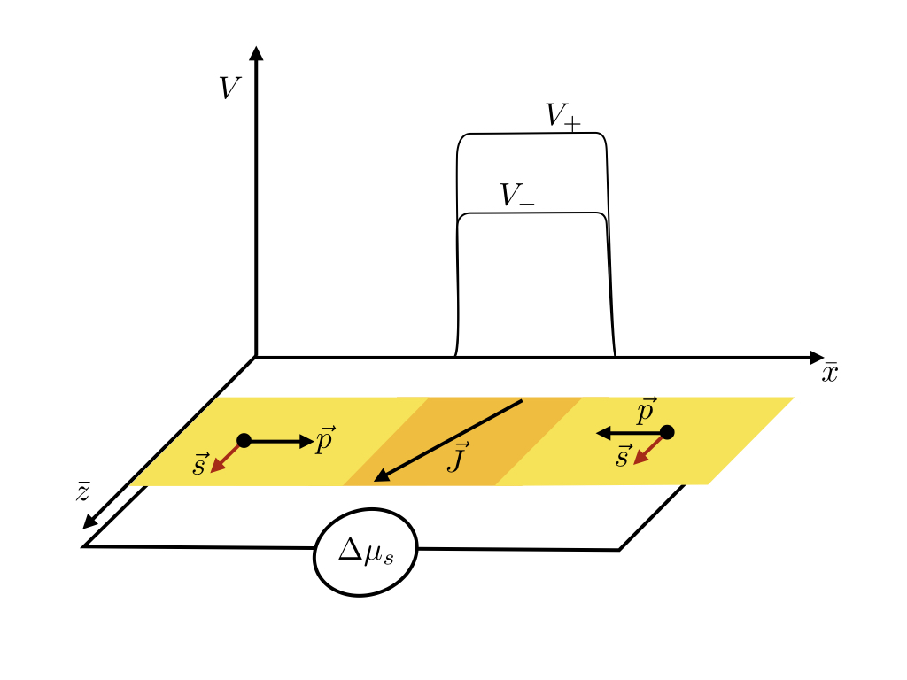
Figure 1: Conceptual scheme of the device. Electrons move across a magnet with total angular momentum $\vec{J}$ under the action of a spin potential difference $\Delta\mu_{s}$. In the magnetic region, they experience a spin-dependent potential $V_{+}:=d\cdot(\lambda_{0}+J\,\lambda/2)$ and $V_{-}:=d\cdot(\lambda_{0}-J\,\lambda/2)$, depending whether their spin is parallel or anti-parallel to the magnetization vector $\vec{J}$, where $d$ is the magnet length.

A generic observable will evolve in time with the propagator $\hat{U}_{t,t_{0}}$ from the initial time $t_{0}$ to an arbitrary time $t$:

$$\langle\hat{O}(t)\rangle=\operatorname{tr}\left[\hat{U}_{t,t_{0}}^{\dagger}\,\hat{O}\,\hat{U}_{t,t_{0}}\,\hat{\rho}(t_{0})\right],$$ (2)

where $\hat{\rho}(t_{0})$ is the density matrix for the initial state of the system, and $\hat{U}_{t,t_{0}}^{\dagger}=\hat{U}_{t_{0},t}$. The Keldysh method thus exploits this symmetry to introduce forward and backward paths in time; the expectation value (2) is obtained by means of an action $S$ and a function $O$, integrated over bosonic and fermionic degrees of freedom:

$$\langle\hat{O}(t)\rangle=\int D[\bar{b}_{+},\bar{b}_{-},\bar{\psi}_{+},\bar{\psi}_{-},b_{+},b_{-},\psi_{+},\psi_{-}]\,O\,e^{i\,S}$$ (3)

where the complex variable $b_{\pm}$ and its conjugate $\bar{b}_{\pm}$ refer to the bosonic field, and the Grassman numbers $\psi_{\pm},\,\bar{\psi}_{\pm}$ refer to the fermionic field. The integration is carried out over the paths $t\to b_{\pm}(t)$ and $t\to\psi_{\pm}(t)$ in both the forward (+) and backward (-) direction of the propagation in time. This formalism produces four propagators in time, two for each time branch and two connecting across them, only three of which are independent. For bosons, the number of propagators is reduced by the Keldysh rotation Keldysh (1965):

$$b^{\text{cl}}=\frac{b^{+}+b^{-}}{\sqrt{2}},\qquad b^{\text{q}}=\frac{b^{+}-b^{-}}{\sqrt{2}},$$ (4a)

$$\bar{b}^{\text{cl}}=\frac{\bar{b}^{+}+\bar{b}^{-}}{\sqrt{2}},\qquad\bar{b}^{\text{q}}=\frac{\bar{b}^{+}-\bar{b}^{-}}{\sqrt{2}}.$$ (4b)

going under the name of classical and quantum parts, respectively.

In our case, the fermionic degrees of freedom are the variables of the electrons, and we can treat the magnet spin $J$ as a bosonic field by means of a Holstein-Primakoff (HP) transformation Holstein and Primakoff (1940):

$$\hat{J}_{+}:=J\left(\sqrt{2-\frac{\hat{b}^{\dagger}\,\hat{b}}{J}}\right)\frac{\hat{b}}{\sqrt{J}},$$ (5a)

$$\hat{J}_{-}:=J\,\frac{\hat{b}^{\dagger}}{\sqrt{J}}\left(\sqrt{2-\frac{\hat{b}^{\dagger}\,\hat{b}}{J}}\right),$$ (5b)

$$\hat{J}_{z}:=J-\hat{b}^{\dagger}\,\hat{b}$$ (5c)

where $\hat{b}^{\dagger}$ and $\hat{b}$ are bosonic creation and annihilation operators obeying canonical commutation rules.

The zero-boson state hence represents the classical limit in which the nano-magnet is perfectly aligned to a given axis, identified with $\hat{z}$. The presence of boson excitations introduces quantum fluctuations of the magnet spin around this classical axis. In this representation, the interaction between the magnet and the electrons can be depicted by the Feynman vertices in Fig. 2a and b: the one-boson vertex is of the order $1/\sqrt{J}$, while the two-boson vertex is of the order $1/J$. For a typical nanomagnet Wang and Sham (2013), we can consider only the terms up to the $1/J$-order, that is the Feynman diagrams shown in Fig. 2c-e. This allows to consider the semiclassical limit of the HP transformation as:

$$\hat{J}_{+}=\sqrt{2\,J}\,\hat{b}+O\left(\frac{1}{\sqrt{J}}\right),$$ (6a)

$$\hat{J}_{-}=\sqrt{2\,J}\,\hat{b}^{\dagger}+O\left(\frac{1}{\sqrt{J}}\right),$$ (6b)

$$\hat{J}_{z}=J-\hat{b}^{\dagger}\,\hat{b}.$$ (6c)

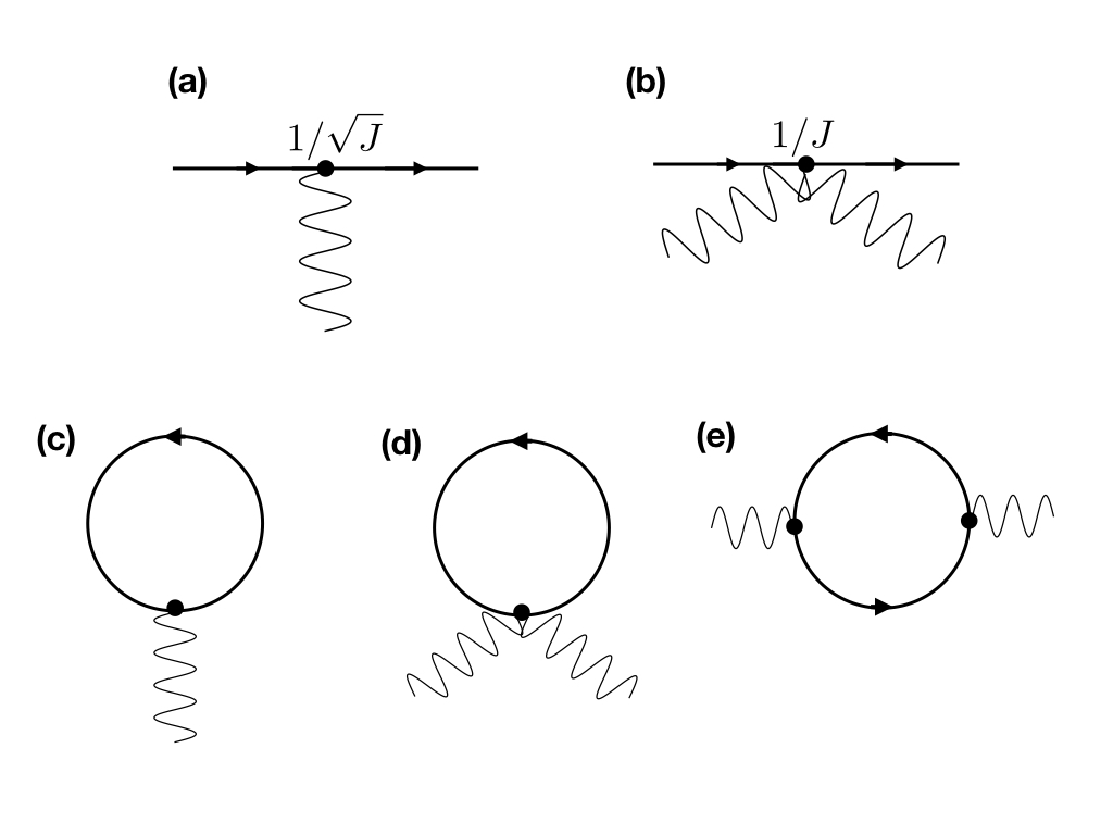
Figure 2: Feynman vertices and diagrams included in our expansion. (a) single-boson vertex, (b) two-boson vertex, (c) “tadpole” diagram (d), (e) boson self-energy diagrams.

In order to derive the equation of motion for the magnetization, we have proceeded as follows Kamenev and Levchenko (2009); Kamenev (2011). The Hamiltonian (1) has been rewritten taking into account explicitly the linearised HP transformation (6), and three terms have been recognised: $H_{\text{0e}}{=}-\frac{\partial_{\bar{x}}^{2}}{2\,m}+(\lambda_{0}+\lambda\,Js_{z})\,\delta(\bar{x})$, which contains the electronic part at fixed magnetic spin, $H_{m}=\gamma\frac{J}{2}\left(B_{+}\hat{b}^{\dagger}+B_{-}\hat{b}\right)+\gamma B_{z}\left(J-\hat{b}^{\dagger}\hat{b}\right)$ that describes the coupling of $\vec{J}$ to the magnetic field, and, the interaction term $H_{b}$, containing all the rest. The Hamiltonians $H_{\text{0e}}$ and $H_{m}$ are used to obtain the initial states, then $H_{b}$ is used as a perturbative correction. The electronic degrees of freedom are traced out, originating the corrections represented by the Feynman diagrams in figures 2(c-e). We have thus found a functional integral expression for the magnet observables in the form:

$$\langle \hat{O}(t)\rangle=\int D[I_{1},I_{2}]\,e^{-\int dt\,\frac{I_{1}^{2}(t)+I_{2}^{2}(t)}{2}}$$ (7)

$$\times\int D[\bar{b}^{\text{cl}},\bar{b}^{\text{q}},b^{\text{cl}},b^{\text{q}}]\,O(\bar{b}^{\text{cl}},b^{\text{cl}})$$

$$\times e^{i\left\{\int dt\,\bar{b}^{\text{q}}\left[i\,\partial_{t}b^{\text{cl}}+f(b^{\text{cl}},\theta,I_{1},I_{2})\right]+\text{h.c.}\right\}},$$

where $\theta$ is the angle between the current polarization axis and the magnetization direction $\vec{J}$; the function $f$ is obtained from the sum of the contributions in the Feynman diagrams in figure 2(c-e). The explicit calculations are reported in the Appendix. Here, $I_{1},\,I_{2}$ are two auxiliary time functions that allows us to linearize the Keldysh action with respect to $b^{\text{q}}$ and $\bar{b}^{\text{q}}$ . The semiclassical limit is taken by performing the integration of Eq. (7) with respect to $b^{\text{q}},\bar{b}^{\text{q}}$:

$$\langle\hat{O}(t)\rangle=\int D[I_{1},I_{2}]\,e^{-\int dt\,\frac{I_{1}^{2}(t)+I_{2}^{2}(t)}{2}}\int D[\bar{b}^{\text{cl}},b^{\text{cl}}]\,O(\bar{b}^{\text{cl}},b^{\text{cl}})\delta\left[i\,\partial_{t}b^{\text{cl}}+f(b^{\text{cl}},\theta,I_{1},I_{2})\right]\delta\left[-i\,\partial_{t}\bar{b}^{\text{cl}}+\bar{f}(b^{\text{cl}},\theta,I_{1},I_{2})\right],$$ (8)

where $\delta$ is the Dirac function. This implies that

$$\begin{cases}i\,\partial_{t}b^{\text{cl}}+f(b^{\text{cl}},\theta,I_{1},I_{2})=0,\\ -i\,\partial_{t}\bar{b}^{\text{cl}}+\bar{f}(b^{\text{cl}},\theta,I_{1},I_{2})=0\end{cases}$$ (9)

are the equations of the motion. The generic function $t\mapsto I_{i}(t)$ in the functional integral is weighted by the factor $e^{\int-\frac{I_{1}^{2}(t)+I_{2}^{2}(t)}{2}\,dt}$, as in the Martin-Siggia-Rose action Martin et al. (1973): the weight is the multivariate Gaussian distribution probability, with zero mean value and unitary variance:

$$\langle I_{i}(t)\rangle=0,\qquad\langle I_{i}(t_{1})\,I_{j}(t_{2})\rangle=\delta(t_{1}-t_{2})\,\delta_{ij},$$ (10)

that is, $I_{i}$ must be considered as Langevin terms in the equation of motion. The presence of these stochastic terms is not surprising, since it is the typical situation of the open quantum systems: when some degrees of freedom are traced over, a stochastic behaviour appears.

Finally, the equation of motion for the magnet can be cast in the LLG form, where the coefficients are expressed in terms of microscopic quantities:

$$\partial_{t}\vec{J}=\gamma\,\vec{B}\times\vec{J}+C_{F}\,\hat{z}^{\prime}\times\vec{J}+C_{D}\,\vec{J}\times(\hat{z}^{\prime}\times\vec{J})$$ (11)

where $\hat{z}^{\prime}$ is the polarization axis of the incoming electrons: $\hat{z}^{\prime}\times\vec{J}$ and $\vec{J}\times(\hat{z}^{\prime}\times\vec{J})$ are a field-like and a damping-like term (compare with LLG equation), that produce respectively a precession around the polarization current direction $\hat{z}^{\prime}$ and an alignment to it. The corresponding microscopic coefficients $C_{F}$ and $C_{D}$ are given by:

$$C_{F}=\Re C_{1}+\frac{-\cos\theta\,\Im C_{2}\,I_{1}+\Re C_{2}\,I_{2}}{\sin\theta},$$ (12a)

$$C_{D}=\frac{\Im C_{1}}{J}+\frac{\cos\theta\,\Re C_{2}\,I_{1}+\Im C_{2}\,I_{2}}{\sin\theta\,J},$$ (12b)

where the $C_{i}$ depend on the scattering matrix and increase with the spin potential difference $\Delta\mu_{s}$. In particular, $C_{1}$ is the contribution of the tadpole diagram Fig. 2(c), while $C_{2}$ corresponds to the boson self-energy diagrams which are higher order corrections in $1/\sqrt{J}$ Fig. 2(d-e). This term disappears in the macroscopic limit $J\to+\infty$, while it gives contribution also at zero temperature (both quantum and thermal noise). Comparing our results with the simpler model in Swiebodzinski et al. (2010), we obtained that the scattering of the electrons from the localized magnet results in both field-like and damping-like stochastic correlated terms, as well as a more complex expression for the noise. We may further notice that field-like and damping-like contributions originate from the real (see $\Re C_{1}$ and $\Re C_{2}$) and imaginary (see $\Im C_{1}$ and $\Im C_{2}$) parts of the coefficients $C_{1}$ and $C_{2}$. The presence of the real and imaginary parts is physically due to the different phase shift, upon scattering from the magnet, experienced by electrons with opposite spin orientation. The microscopic coefficients $C_{1}$ and $C_{2}$, whose explicit expression is given in the next Section (see Eqs (14a)-(14b)), are then the result of the interference between the transmission processes for electrons with opposite spin. This interference gives rise to the so-called spin-mixing conductance Brataas et al. (2000), which appears whenever paramagnetic conductors are coupled with ferromagnetic metals.

III Numerical example

We now turn to solving the equation of motion (11) we have obtained in the previous section. It is convenient to tackle this by numerical methods. For a comparison to the results in Ref. Wang and Sham (2013), we adopt in our solution the same parameters and initial conditions. In this example, an external magnetic field $\vec{B}$ is only applied at the beginning of the dynamics, and it is assumed that the timescale for the dynamics is much shorter than any thermalization time: for these reasons, the magnetic field and the temperature are relevant only for determining the initial state. This is the Gibbs ensemble associated to the unperturbed magnet Hamiltonian $H_{m}$ Wang and Sham (2013), characterized by the probability distribution:

$$P(\hat{z},t=0)=C\,e^{-\beta\,E}=C\,e^{\beta\,\vec{M}\cdot\vec{B}}=C\,e^{\beta\,\gamma\,J\,\hat{z}\cdot\vec{B}}$$ (13)

where $E$ is the magnetic energy and $C$ is a normalization constant $C^{-1}={4\,\pi\,\sinh(\beta\,B\,\gamma\,J)}/({\beta\,B\,\gamma\,J})$.

We considered a polarized current along the $\hat{z}^{\prime}$ axis coming from the left to the right: $\Delta\mu_{\text{spin}}^{R}=0$ and $\Delta\mu_{\text{spin}}^{L}=:\Delta\mu_{\text{spin}}$. Under these conditions, we have

$$C_{1}=t_{\downarrow}(k_{F})\,t_{\uparrow}^{\ast}(k_{F})\frac{\Delta\mu_{\text{spin}}\,\lambda\,m\,}{4\,\pi\,k_{F}},$$ (14a)

$$C_{2}=t_{\downarrow}(k_{F})\,t_{\uparrow}^{\ast}(k_{F})\,\lambda\,\sqrt{\frac{\Delta\mu_{\text{spin}}\,m}{\pi\,16\,\epsilon_{F}}},$$ (14b)

where $t_{\uparrow\downarrow}(k_{k})$ is the transmission coefficient for the electrons with spin parallel and anti-parallel with respect to $\vec{J}$, respectively, evaluated at the Fermi wavelength (the calculations are reported in the Appendix). In Wang and Sham (2013) it is assumed that $n_{e}=1.5\cdot 10^{5}$ electrons with fixed spin up come from the left to right in a time $t_{n}$, which is typically of the order of the nanosecond. Since the density current associated to a plane wave $\Psi(\bar{x})=A\,e^{\pm i\,\lvert k\rvert\,\bar{x}}$ is $I=\frac{1}{m}\,\Im\left(\Psi^{\ast}\,\partial_{\bar{x}}\Psi\right)=\pm\frac{1}{m}\,\lvert k\rvert\,\lvert A\rvert^{2}$, we must have $\Delta\mu_{\text{spin}}={2\,\pi\,n_{e}}/{t_{n}}$. The actual numerical values are reported in Table 1.

Element	Value	Dimensions
$t_{\uparrow}(k_{F})$	$0.067-0.251\,i$
$t_{\downarrow}(k_{F})$	$0.924-0.265\,i$
$\Delta\mu_{\text{spin}}$	$$9.990\text{\times}{10}^{-29}\text{\,}\mathrm{J}\text{\,}\mathrm{s}$/t_{n}$	energy
$C_{1}$	$(3.312+5.509\,i)/t_{n}$	time-1
$C_{2}$	$(0.009\,+0.014\,i)/\sqrt{t_{n}}$	time-1/2
$B$	$0.05\text{\,}\mathrm{T}$	magnetic field
$\vec{B}$ direction	$(\theta,\phi)=(2.8,1.0)$
$T$	$1\text{\,}\mathrm{K}$	temperature

Table 1: To reproduce the simulation in Wang and Sham (2013), we consider $\lambda_{0}=3.36\cdot 10^{-28}$\mathrm{J}\,\mathrm{m}$$, $\lambda=5.76\cdot 10^{-32}$\mathrm{J}\,\mathrm{m}$$, $J=10^{4}$ and $k_{F}=13.6\,$\mathrm{n}\mathrm{m}^{-1}$$; furthermore $\Delta\mu_{\text{spin}}=2\,\pi\,\,1.5\cdot 10^{5}/t_{n}$.

With the adopted choice of the numerical values of the parameters $C_{2}^{2}$ is negligible with respect to $C_{1}$ to a first approximation. We will see that this is inappropriate around the switching time $t\sim t_{n}$, and the quantum fluctuations become the main contribution to noise.

Fixing $C_{2}=0$ and choosing the $\theta=0$ axis parallel to the current polarization, the solution of the equation of motion (11) is easily found:

$$\begin{cases}\theta_{S}(t,\theta_{0})=\theta(t)=2\,\cot^{-1}\left[\cot\left(\frac{\theta_{0}}{2}\right)\,e^{\Im C_{1}\,t}\right],\\ \phi_{S}(t,\phi_{0})=\phi(t)=\Re C_{1}\,t+\phi_{0},\end{cases}$$ (15)

where $\theta_{0}$ and $\phi_{0}$ are the angles for $t=0$. Observe that $\theta(t)$ is a decreasing function that, for $t\to+\infty$, goes to $0$; this represents the damping effect. The trajectory of the average (over all the possible pairs of initial values $\theta_{0}$ and $\phi_{0}$ chosen in the Gibbs ensemble of Eq. (13)) value of $\vec{J}$ is traced in Fig. 3.

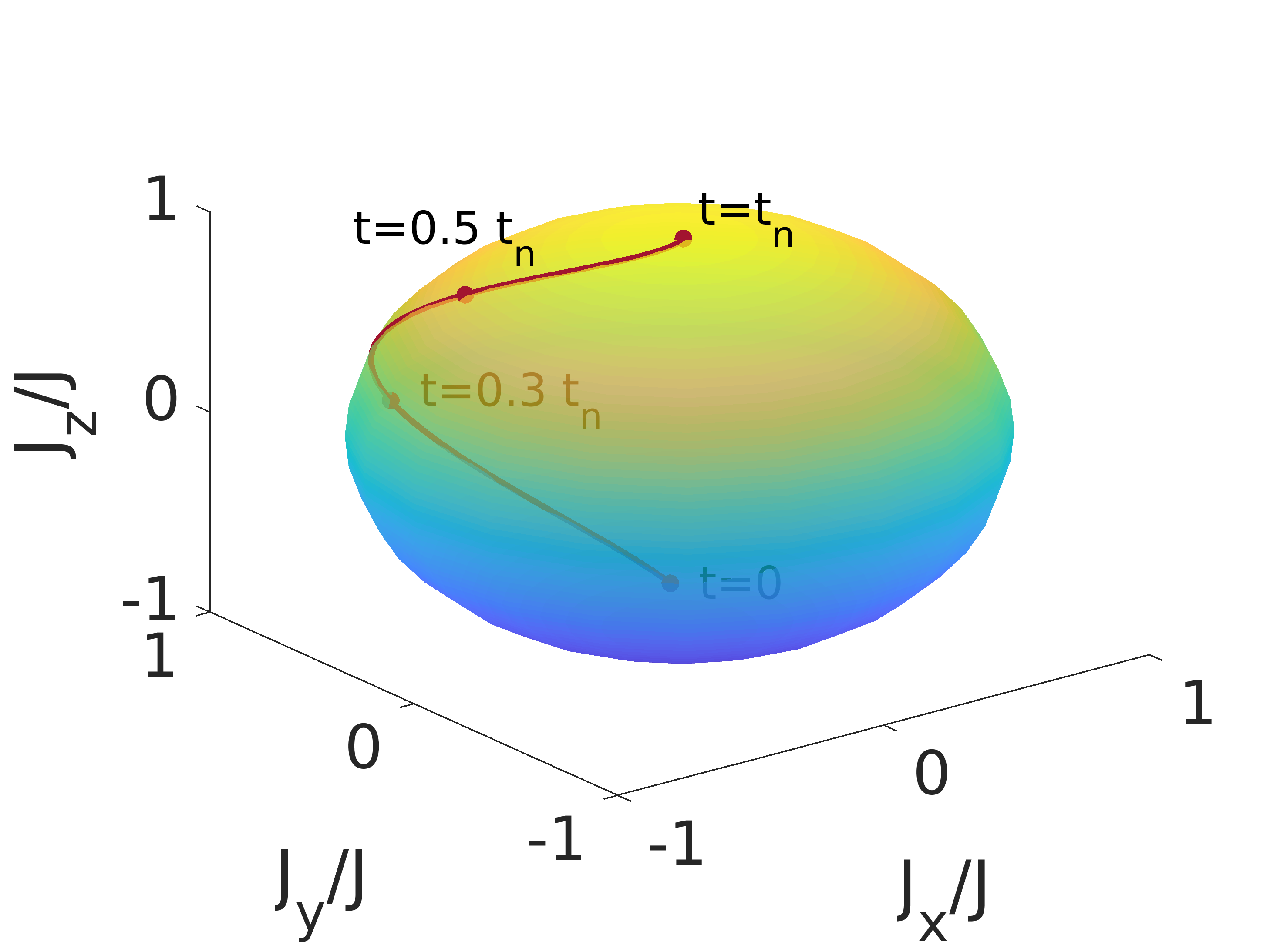
Figure 3: Mean value trajectory of $\vec{J}/J$ during the time interval $[0,t_{n}]$.

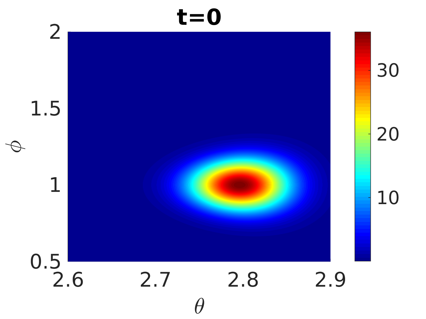
(a) The initial probability distribution.

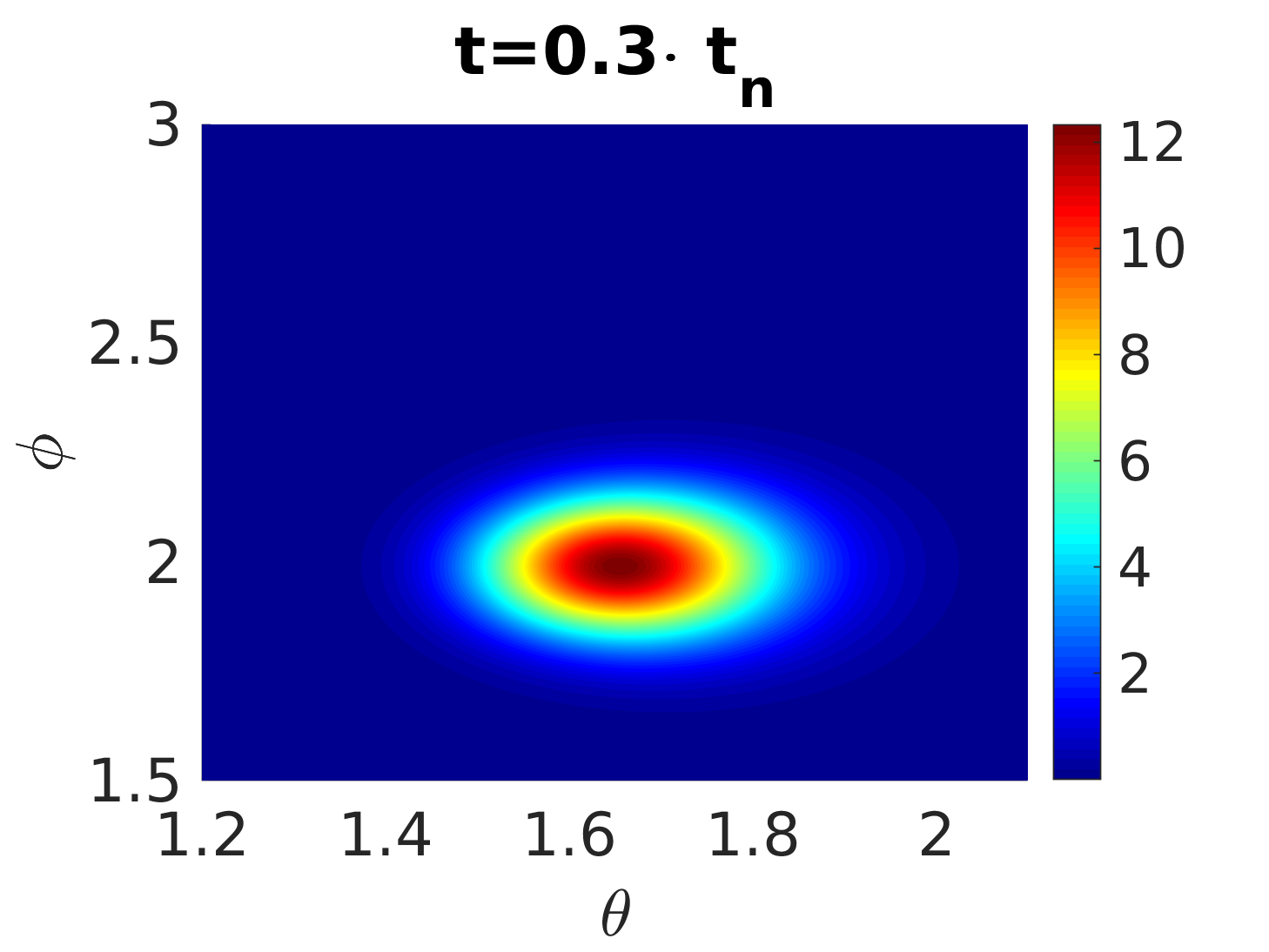
(b) The distribution for $t=0.3\cdot t_{n}$.

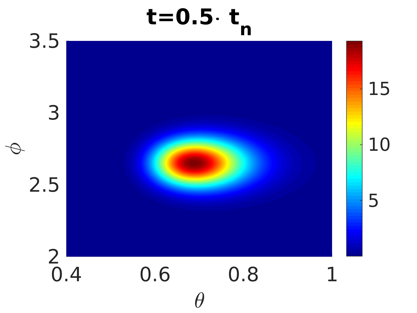
(c) The distribution for $t=0.5\cdot t_{n}$.

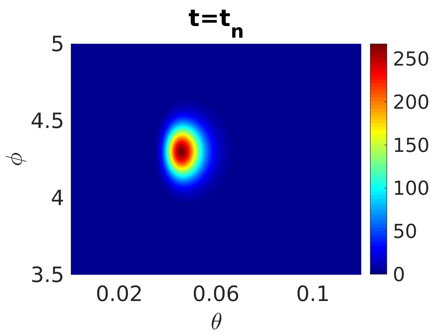
(d) The distribution for $t=t_{n}$.

Figure 4: The probability distribution for $(\theta,\phi)$ in radians.

We take into account the fluctuations of $J$ in Fig. 4, where we show the time-dependent probability distribution $p(\theta,\phi;t)$, with the initial condition $p_{0}(\theta,\phi)=p(\theta,\phi;t=0)=P(\hat{z},t=0)\,\sin\theta$. The time evolution for $p(\theta,\phi)$ is derived by considering the evolution of each trajectory:

$$p(\theta,\phi;t) = p_{0}[\theta_{S}(-t,\theta),\phi_{S}(-t,\phi)]$$ (16)

$$\times\biggl{\lvert}\frac{\partial[\theta_{S}(-t,\theta),\phi_{S}(-t,\phi)]}{\partial(\theta,\phi)}\biggr{\rvert},$$

where $\lvert\partial(\theta_{S},\phi_{S})/\partial(\theta,\phi)\rvert$ is the absolute value of the Jacobian determinant; this expression has been used to obtain the contour plots in Fig. 4.

The mean value and the standard deviation of the three components of $\vec{J}$ are summarized in the plots of Fig. 5b, where they are represented as a function of time. As expected based on the values of $C_{1}$ and $C_{2}^{2}$, these figures are similar to the analogous ones in Ref. Wang and Sham (2013); in particular, the behaviour of the fluctuations in Fig. 5b is mostly due to the propagation of the initial fluctuations. The only discrepancy in this comparison is the fact that the probability density in Fig. 4d shows smaller fluctuations. This is not surprising, since for large $t$ damping suppresses all the fluctuations because all the trajectories converge to $\theta=0$: the quantum noise becomes relevant.

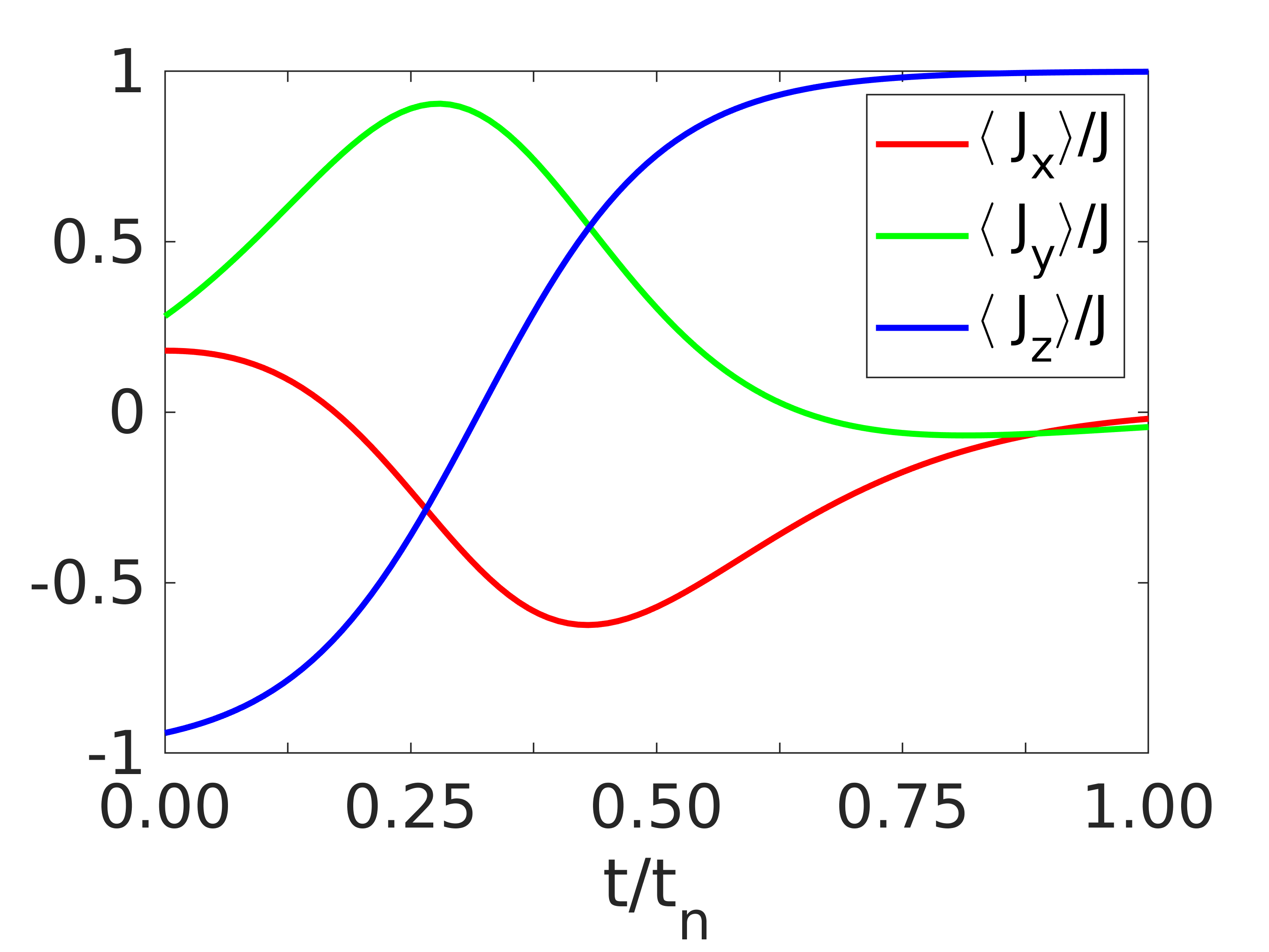
(a) Mean value.

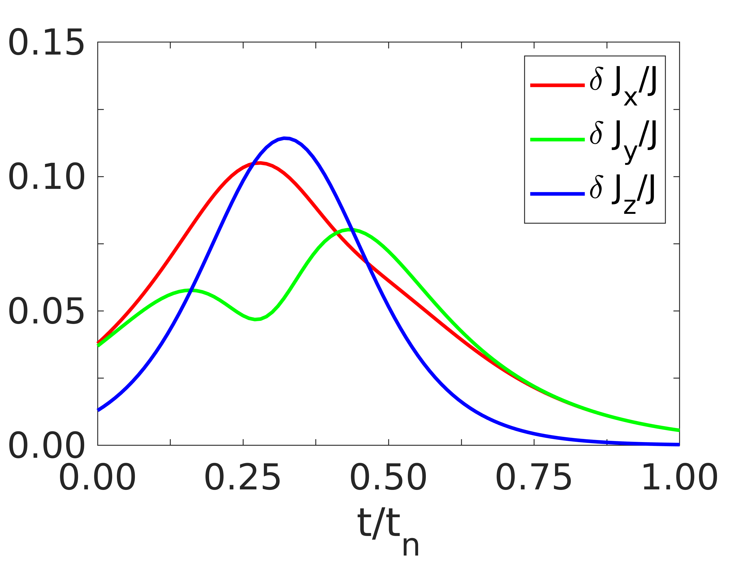
(b) Fluctuation.

Figure 5: Mean value and standard deviation of $\vec{J}/J$ during the time interval $[0,t_{n}]$.

As anticipated, quantum fluctuations become important in the long-time limit, in which, due to damping, the angle $\theta(t)$ remains close to $\theta=0$, i.e. the magnet is almost aligned to the spin of the current. This allows to derive two equations for $\theta$ and $\phi$ from the Eq. (11) as

$$\theta^{\prime}(t)=-\Im C_{1}\,\sin\theta-\left[I_{1}(t)\,\Re C_{2}\,\cos\theta+I_{2}(t)\,\Im C_{2}\right],$$

(17a)

$$\phi^{\prime}(t)=\Re C_{1}-\frac{I_{1}(t)\,\Im C_{2}\,\cos\theta-I_{2}(t)\,\Re C_{2}}{\sin\theta}.$$ (17b)

The first equation can be linearised with respect to $\theta$ by taking the small angle approximation:

$$\theta^{\prime}(t)\simeq-\Im C_{1}\,\theta-I_{1}(t)\,\Re C_{2}-I_{2}(t)\,\Im C_{2}.$$ (18)

Since the last term is a linear combination of two independent Gaussian stochastic processes, it can be cast as a single one with average $\langle I(t)\rangle=0$ and correlation $\langle I(t_{1})\,I(t_{2})\rangle=\lvert C_{2}\rvert^{2}\,\delta(t_{1}-t_{2})$. Therefore, Eq. (18) reduces to an Ornstein-Uhlenbeck process, whose corresponding Fokker-Planck equation is:

$$\partial_{t}p(\theta,t)=\Im C_{1}\,\partial_{\theta}[\theta\,p(\theta,t)]+\frac{\lvert C_{2}\rvert^{2}}{2}\,\partial_{\theta}^{2}p(\theta,t),$$ (19)

whose stationary solution is a Gaussian distribution with zero mean value and variance $\lvert C_{2}\rvert^{2}/(2\,\Im C_{1})$. We refer to the Appendix for the details on the derivation. The variance is of the order $\simeq 5\cdot 10^{-5}$ in our numerical example, thus giving a standard deviation consistent with the difference between our figure 4d and the numerical solution in Ref. Wang and Sham (2013).

The dynamic equation for $\phi$ (17b) has a similar structure:

$$\phi^{\prime}(t)=\Re C_{1}+\tilde{I}(t),$$ (20)

governed by a stochastic process with $\langle\tilde{I}(t)\rangle=0$, and $\langle\tilde{I}(t_{1})\,\tilde{I}(t_{2})\rangle=\delta(t_{1}-t_{2})\,\frac{\Im C_{2}^{2}\,\cos^{2}\theta+\Re C_{2}^{2}}{\sin^{2}\theta}.$ The variance at $\theta=0$ diverges, as one could expect since in this limit the angle $\phi$ is not defined anymore, thus ensuring that the trajectory $t\mapsto(\theta(t),\phi(t))$ of the stochastic process remains continuous. We also remark that in Refs. Wang and Sham (2012, 2013) the diffusion constant for the nano-magnet has been estimated to be of the order of ${10}^{5}\text{\,}\mathrm{s}^{-1}$, which is comparable with the thermal noise at $T\sim$3\text{\,}\mathrm{K}$$ Wang and Sham (2012); Brown Jr (1963)). This is also captured by out treatment: for a flipping time $t_{n}\sim$1\text{\,}\mathrm{ns}$$, we find $\lvert C_{2}\rvert^{2}\sim$3\text{\times}{10}^{5}\text{\,}\mathrm{s}^{-1}$$.

In our derivation we have assumed that the full system consisting of the electrons and the nano-magnet is not isolated: such interaction with the environment (or with a continuously measuring device) enforces it not to remain in a superposition of different positions Joos and Zeh (1985); Zurek (2003); Breuer et al. (2002). In principle, however, the Keldysh formalism can be exploited also when relaxing this assumption (refer to the Appendix).

IV Conclusion

We have introduced a simple model for the description of noise in STT based on the Keldysh technique. This has allowed us to derive the equation of motion for a nanomagnet interacting with a spin-polarized current; for each term we are able to trace a microscopic origin, and we have made an explicit connection with the spin mixing conductance. We found a good agreement with the model in Wang and Sham (2012), focusing on the scattering matrix approach in the relevant limit.

Thanks to this versatile method, one can extend the treatment to more involved examples, such as those addressing multiple magnets and their correlation that find application in the read/write process, and potential extension to quantum information processing in a solid state architecture.

Appendix A The many-body model

As in Ref. Wang and Sham (2013), we considered electrons only moving in the $\bar{x}$ direction. In principle, the model of Eq. (1) is easily generalizable: if the electric current flows in a device with nanometric transverse dimensions, one can quantize the electron state along $\bar{y}$ and $\bar{z}$ and consider the eigenstates along these directions as current channels Nazarov and Blanter (2009). The only complication is that the magnetic scattering center in $\bar{x}=0$ would produces mixing between the channels.

The Keldysh formalism will allow us to treat that model directly in the many-body framework, provided that we translate the magnet degrees of freedom in terms of boson fields. As in Ref. Swiebodzinski et al. (2010), we will consider the Holstein-Primakoff bosonization defined in Eq.(5). By this we consider a semi-classical approximation for the magnet dynamics, in the limit of large $J$ and slight deviation from a coherent state. We then confine to states that are thus combination of few bosons states to ensure that the condition $\langle\hat{J}_{x,y}\rangle\ll J$) holds. In turn, this implies that

$$\frac{\langle\hat{b}\rangle}{\sqrt{J}},\,\frac{\langle\hat{b}^{\dagger}\rangle}{\sqrt{J}}=O\left(\frac{1}{\sqrt{J}}\right),\qquad\langle\hat{b}^{\dagger}\,\hat{b}\rangle\ll J.$$ (21)

The many-body Hamiltonian $\hat{H}=\hat{H}_{\text{m}}+\hat{H}_{\text{0e}}+\hat{H}_{b}$ is then rewritten in this limit.

The starting point is to identify the scattering states associated to the electronic Hamiltonian $\hat{H}_{\text{0e}}$ Nazarov and Blanter (2009):

$$\Psi {}_{\lvert k\rvert s}(x)=N$$ (22a)

$$\times\begin{cases}\Ket{s}e^{i\,\lvert k\rvert\,\bar{x}}+\hat{r}(k)\ket{s}e^{-i\,\lvert k\rvert\,\bar{x}},&\bar{x}<0,\\ \hat{t}(k)\Ket{s}e^{i\,\lvert k\rvert\,\bar{x}},&\bar{x}>0,\end{cases}$$

$$\Psi {}_{-\lvert k\rvert s}(x)=N$$ (22b)

$$\times\begin{cases}\hat{t}(k)\Ket{s}e^{-i\,\lvert k\rvert\,\bar{x}},&\bar{x}<0,\\ \Ket{s}e^{-i\,\lvert k\rvert\,\bar{x}}+\hat{r}(k)\Ket{s}e^{i\,\lvert k\rvert\,\bar{x}},&\bar{x}>0.\end{cases}$$

Here $N$ is a real normalization constant  and $\Ket{s}$ are spinors. This implies that the transmittivity and reflectivity coefficients are spinor operators in the form

$$\Braket{s_{1}}{\hat{r}(k)}{s_{2}}=\begin{pmatrix}r_{\uparrow}(k)&0\\ 0&r_{\downarrow}(k)\end{pmatrix},$$ (23a)

$$\Braket{s_{1}}{\hat{t}(k)}{s_{2}}=\begin{pmatrix}t_{\uparrow}(k)&0\\ 0&t_{\downarrow}(k)\end{pmatrix}$$ (23b)

with respect to the $\hat{z}$-quantization axis and

$$r_{s}(k)=\frac{1}{-1+i\,\frac{\lvert k\rvert}{m\,(\lambda_{0}+\lambda\,s\,J/2)}},$$ (24a)

$$t_{s}(k)=\frac{1}{1+i\,\frac{m\,(\lambda_{0}+\lambda\,s\,J/2)}{\lvert k\rvert}};$$ (24b)

for convenience we will use the notations $s=\uparrow\downarrow$ and $s=\pm$ with the same meaning. The states $\Psi_{ks}$ constitute a basis for electrons (respectively coming from left to right and from right to left):

$$\hat{H}_{\text{0e}}\Psi_{ks}=\epsilon_{ks}\,\Psi_{ks},\quad\epsilon_{ks}=\epsilon_{k}=\frac{k^{2}}{2\,m},\quad s=\pm.$$ (25)

Then the many-electron free Hamiltonian is written as

$$\hat{H}_{\text{0e}}=\sum_{ks}\epsilon_{k}\,\hat{c}_{ks}^{\dagger}\,\hat{c}_{ks},$$ (26)

where $\hat{c}_{ks}$ creates an electron in the state $\Psi_{ks}$. We stress that the choice to consider an expansion based on the scattering eigenfunctions $\Psi_{ks}$ is a key technical point to be exploited later on in our discussion.

The interaction term $\hat{H}_{b}$ containing the $\hat{b},\,\hat{b}^{\dagger}$ operators can be considered as a perturbation. Indeed, while $\hat{H}_{\text{0e}}$ contains the terms $\lambda_{0}$ and $\lambda\,J$ (that can be even considered of the similar order – see Fig. 1), it is easy to check that $\hat{H}_{b}$ is given by the sum of terms that contain a single bosonic operator ($\hat{b}$ or $\hat{b}^{\dagger}$) which is of the order $\lambda\,\sqrt{J}$ (and then suppressed by a factor $1/\sqrt{J}$ with respect to $\lambda\,J$) and a term proportional to $\hat{b}\,\hat{b}^{\dagger}$ which is of the order $\lambda$ (and then suppressed by a factor $1/J$ with respect to $\lambda\,J$).

The incoming current is polarized with respect to an axis denoted $\hat{z}^{\prime}$ to distinguish it from the one of the magnet $\hat{z}$. The spin states in these two reference frames are related by the rotation

$$\hat{U}(\theta,\phi)\Ket{s}=\Ket{s^{\prime}},$$ (27a)

$$\Braket{s_{1}^{\prime}}{\hat{U}}{s_{2}^{\prime}}=\Braket{s_{1}}{\hat{U}}{s_{2}}$$

$$\quad=\begin{pmatrix}e^{-i\,\phi/2}\,\cos\frac{\theta}{2}&-e^{-i\,\phi/2}\,\sin\frac{\theta}{2}\\ e^{i\,\phi/2}\,\sin\frac{\theta}{2}&e^{i\,\phi/2}\,\cos\frac{\theta}{2}\end{pmatrix}$$ (27b)

where $\hat{U}=e^{-i\,\hat{s}_{z}\,\phi}\,e^{-i\,\hat{s}_{y}\,\theta}$, with polar and azimuthal angle $\theta$ and $\phi$, respectively. The creation operator $\hat{c}_{ks}^{\dagger}$ is associated to an electron in the state $\Ket{k,s}$, and similarly for $\hat{c}_{ks^{\prime}}^{\dagger}$:

$$\hat{c}^{\dagger}_{ks_{1}}=\sum_{s_{2}^{\prime}}\Braket{s_{2}^{\prime}}{s_{1}}\hat{c}_{ks_{2}^{\prime}}^{\dagger}=\sum_{s_{2}^{\prime}}\Braket{s_{2}^{\prime}}{\hat{U}^{\dagger}}{s_{1}^{\prime}}\hat{c}_{ks_{2}^{\prime}}^{\dagger}.$$ (28)

Since the eigenvalues of $H_{\text{0e}}$ do not depend on $s$, we may write the electronic Hamiltonian (26) in the same form in the two reference frames.

Then we assume that the incoming electrons density matrix is that of a thermal state

$$\hat{\rho}_{0}^{s^{\prime},d}=\frac{1}{\mathcal{Z}_{s^{\prime},d}}\,\exp\left[-\beta\sum_{k}\left(\epsilon_{k}-\mu^{s^{\prime},d}\right)\hat{c}_{d\lvert k\rvert,s^{\prime}}^{\dagger}\cdot\hat{c}_{d\lvert k\rvert,s^{\prime}}\right],$$ (29)

where the index $d=\pm$ describes the direction of the electronic motion .

The operator that annihilates (creates) an electron in $x$ with spin $s$ is given by

$$\hat{\psi}_{s}(x)=\sum_{k}\Psi_{ks}(x;s)\,c_{ks},\quad\hat{\psi}_{s}^{\dagger}(x)=\sum_{k}\Psi_{ks}^{\ast}(x;s)\,c^{\dagger}_{ks},$$ (31)

where $\Psi_{ks}(x;s):=\Bra{s}\Psi_{ks}(x)$, therefore

$$\hat{\psi}_{s}(0)=N\sum_{k}t_{s}(k)\,c_{ks},\quad\hat{\psi}^{\dagger}_{s}(0)=N\sum_{k}t_{s}^{\ast}(k)\,c^{\dagger}_{ks}.$$ (32)

The interaction Hamiltonian can then be written as

$$\hat{H}_{b} = \lambda\sum_{s_{1}s_{2}}\int d\bar{x}\Bigl{[}-\frac{1}{2}\,\hat{b}^{\dagger}\,\hat{b}\,\sigma^{3}_{s_{2}s_{1}}+\frac{\sqrt{2\,J}}{2}\,\sigma^{+}_{s_{2}s_{1}}\,\hat{b}^{\dagger}$$ (33)

$$+\frac{\sqrt{2\,J}}{2}\,\sigma^{-}_{s_{2}s_{1}}\,\hat{b}\Bigr{]}\hat{\psi}^{\dagger}_{s_{2}}(\bar{x})\,\hat{\psi}_{s_{1}}(\bar{x})\,\delta(\bar{x}),$$

where $\sigma^{1},\sigma^{2},\sigma^{3}$ are the Pauli matrices, and $\sigma^{\pm}=\sigma^{1}\pm i\sigma^{2}$. This contains a degeneration lifting of the two spin levels, as well as Jaynes-Cummings terms. These describe the situation in which the spin flip of an electron creates or annihilates a bosonic excitation, accounting for the conservation of the total angular momentum. Integration over $\bar{x}$ gives the expression

$$\hat{H} {}_{b}=\sum_{s_{2}^{\prime}s_{1}^{\prime}k_{2}k_{1}}\biggl{\{}\hat{b}^{\dagger}\,\hat{b}\,\mathcal{M}_{k_{2}k_{1}}^{s_{2}s_{1}}(\parallel)\,\hat{c}_{k_{2}s_{2}^{\prime}}^{\dagger}\,\hat{c}_{k_{1}s_{1}^{\prime}}$$ (34)

$$+\left[\hat{b}\,\mathcal{M}_{k_{2}k_{1}}^{s_{2}s_{1}}(\bot)\,\hat{c}_{k_{2}s_{2}^{\prime}}^{\dagger}\,\hat{c}_{k_{1}s_{1}^{\prime}}+\text{h.c.}\right]\biggr{\}}$$

$$=H_{b\parallel}+H_{b\perp},$$

where we have also used the basis transformation (28). The Hamiltonian can be separated into two contributions, depending on the relative orientation with respect to the $\hat{z}$ axis. The coefficient of the parallel contribution is given by

$$\mathcal{M}^{s_{2}^{\prime}\,s_{1}^{\prime}}_{k_{2}\,k_{1}}(\parallel) := -\frac{\lambda}{4}\,N^{2}\Bigl{[}t^{\ast}_{+}(k_{2})\,t_{+}(k_{1})\,\mathcal{L}_{+}^{s_{2}^{\prime}s_{1}^{\prime}}(\parallel)$$ (35)

$$+t^{\ast}_{-}(k_{2})\,t_{-}(k_{1})\,\mathcal{L}_{-}^{s_{2}^{\prime}s_{1}^{\prime}}(\parallel)\Bigr{]},$$

with

$$\mathcal{L}_{+}^{s_{2}^{\prime}s_{1}^{\prime}}(\parallel)=\begin{pmatrix}1+\cos\theta&-\sin\theta\\ -\sin\theta&1-\cos\theta\end{pmatrix},$$ (36a)

$$\mathcal{L}_{-}^{s_{2}^{\prime}s_{1}^{\prime}}(\parallel)=\begin{pmatrix}\cos\theta-1&-\sin\theta\\ -\sin\theta&-1-\cos\theta\end{pmatrix}.$$ (36b)

This term is associated to the vertex in Fig. 2(b). The coefficient for the perpendicular contribution is

$$\mathcal{M}^{s_{2}^{\prime}\,s_{1}^{\prime}}_{k_{2}\,k_{1}}(\bot)=\lambda\,\frac{\sqrt{2\,J}}{2}\,N^{2}\,t_{-}^{\ast}(k_{2})\,t_{+}(k_{1})\,\mathcal{L}^{s_{2}^{\prime}s_{1}^{\prime}}(\bot),$$ (37)

with

$$\mathcal{L}^{s_{2}^{\prime}s_{1}^{\prime}}(\bot)=e^{-i\,\phi}\,\begin{pmatrix}\frac{\sin\theta}{2}&-\sin^{2}\frac{\theta}{2}\\ \cos^{2}\frac{\theta}{2}&-\frac{\sin\theta}{2}.\end{pmatrix}.$$ (38)

This term is associated to the vertex in Fig. 2(a).

Appendix B Keldysh action

In the Keldysh formalism Kamenev and Levchenko (2009), the magnet-electron action for our system is given by

$$S =\int_{-\infty}^{+\infty}dt\biggl{(}\bar{b}_{+}\,i\,\partial_{t}\,b_{+}+\sum_{ks^{\prime}}(\bar{\psi}_{+})_{ks^{\prime}}\,i\,\partial_{t}\,(\psi_{+})_{ks^{\prime}}$$ (39)

$$-H[\bar{b}_{+},\bar{\psi}_{+},b_{+},\psi_{+}]\biggr{)}$$

$$-\int_{-\infty}^{+\infty}dt\biggl{(}\bar{b}_{-}\,i\,\partial_{t}\,b_{-}+\sum_{ks^{\prime}}(\bar{\psi}_{-})_{ks^{\prime}}\,i\,\partial_{t}\,(\psi_{-})_{ks^{\prime}}$$

$$-H[\bar{b}_{-},\bar{\psi}_{-},b_{-},\psi_{-}]\biggr{)}=\int dt\,\mathcal{L}$$

where $b_{\pm}$ are numbers that correspond to the bosonic degrees of freedom and $\psi_{\pm}$ are Grassmann numbers for fermions modes. The Keldysh rotation can be applied to reduce the number of propagators: we apply the rotation (4) for bosons, while for fermions we use the Larkin-Ovchinnikov notation Kamenev and Levchenko (2009):

$$\psi_{1}=\frac{\psi_{+}+\psi_{-}}{\sqrt{2}},\qquad\psi_{2}=\frac{\psi_{+}-\psi_{-}}{\sqrt{2}},$$ (40a)

$$\bar{\psi}_{1}=\frac{\bar{\psi}_{+}-\bar{\psi}_{-}}{\sqrt{2}},\qquad\bar{\psi}_{2}=\frac{\bar{\psi}_{+}+\bar{\psi}_{-}}{\sqrt{2}}.$$ (40b)

The action is the sum of four components: $S_{m}$, $S_{\text{0e}}$, $S_{b\parallel}$, $S_{b\perp}$. The first term of the Lagrangian $\mathcal{L}$ contains terms associated to the magnet only:

$$\mathcal{L}_{m}=\bar{b}_{+}\,i\,\partial_{t}\,b_{+}-H_{m}[\bar{b}_{+},b_{+}]-\bar{b}_{-}\,i\,\partial_{t}\,b_{-}+H_{m}[\bar{b}_{-},b_{-}],$$ (41)

which yields the action:

$$S {}_{m}=\int dt\,\begin{pmatrix}\bar{b}^{\text{cl}}&\bar{b}^{\text{q}}\end{pmatrix}\begin{pmatrix}0&i\,\partial_{t}+\gamma\,B_{z}\\ i\,\partial_{t}+\gamma\,B_{z}&0\end{pmatrix}\begin{pmatrix}b^{\text{cl}}\\ b^{\text{q}}\end{pmatrix}$$

$$-\int dt\left[\frac{\gamma\,\sqrt{J}}{\sqrt{2}}\,B_{+}\left(\bar{b}_{+}-\bar{b}_{-}\right)+\frac{\gamma\,\sqrt{J}}{\sqrt{2}}\,B_{-}\left(b_{+}-b_{-}\right)\right]$$

$$=\int dt\left[\bar{b}^{\text{q}}\left(i\,\partial_{t}+\gamma\,B_{z}\right)b^{\text{cl}}-\gamma\,\sqrt{J}\,B_{+}\,\bar{b}^{\text{q}}\right]+\text{h.c.},$$

where the first integral has been evaluated by parts.

The purely electronic contribution is written as

$$\mathcal{L}_{\text{0e}} = \sum_{ks^{\prime}}(\bar{\psi}_{+})_{ks^{\prime}}\,i\,\partial_{t}\,(\psi_{+})_{ks^{\prime}}-H_{0e}[\bar{\psi}_{+},\psi_{+}]$$

$$-\sum_{ks^{\prime}}(\bar{\psi}_{-})_{ks^{\prime}}\,i\,\partial_{t}\,(\psi_{-})_{ks^{\prime}}+H_{0e}[\bar{\psi}_{-},\psi_{-}].$$

For both arms of the Keldysh contours, the Grassman numbers are indexed to take into account the spin, the direction of the electronic motion, and the momentum. We then introduce:

$$\bar{\psi}=\biggl{(} \begin{matrix}\begin{pmatrix}\bar{\psi}_{1\uparrow^{\prime}+}&\bar{\psi}_{2\uparrow^{\prime}+}\end{pmatrix}&\begin{pmatrix}\bar{\psi}_{1\downarrow^{\prime}+}&\bar{\psi}_{2\downarrow^{\prime}+}\end{pmatrix}\end{matrix}$$ (44)

$$\begin{matrix}\begin{pmatrix}\bar{\psi}_{1\uparrow^{\prime}-}&\bar{\psi}_{2\uparrow^{\prime}-}\end{pmatrix}&\begin{pmatrix}\bar{\psi}_{1\downarrow^{\prime}-}&\bar{\psi}_{2\downarrow^{\prime}-}\end{pmatrix}\end{matrix}\biggr{)}$$

and

$$\psi=\begin{pmatrix}\begin{pmatrix}\psi_{1\uparrow^{\prime}+}\\ \psi_{2\uparrow^{\prime}+}\end{pmatrix}\\ \begin{pmatrix}\psi_{1\downarrow^{\prime}+}\\ \psi_{2\downarrow^{\prime}+}\end{pmatrix}\\ \begin{pmatrix}\psi_{1\uparrow^{\prime}-}\\ \psi_{2\uparrow^{\prime}-}\end{pmatrix}\\ \begin{pmatrix}\psi_{1\downarrow^{\prime}-}\\ \psi_{2\downarrow^{\prime}-}\end{pmatrix}\end{pmatrix},$$ (45)

where $\uparrow^{\prime}\downarrow^{\prime}$ refer to spin along $\hat{z}^{\prime}$, $\pm$ to the electron motion direction and each $\psi_{is^{\prime}d}$ is a block indexed by the momentum $\lvert k\rvert$:

$$\bar{\psi}_{is^{\prime}\pm}=\begin{pmatrix}\bar{\psi}_{is^{\prime}\pm\lvert k_{1}\rvert}&\bar{\psi}_{is^{\prime}\pm\lvert k_{2}\rvert}&\cdots\end{pmatrix},$$ (46a)

$$\psi_{is^{\prime}\pm}=\begin{pmatrix}\psi_{is^{\prime}\pm\lvert k_{1}\rvert}\\ \psi_{is^{\prime}\pm\lvert k_{2}\rvert}\\ \vdots\end{pmatrix}.$$ (46b)

With this notation, the electronic action is written as

$$S_{\text{0e}}=\int dt\,\sum_{ks}\begin{pmatrix}\bar{\psi}_{1ks}&\bar{\psi}_{2ks}\end{pmatrix}\begin{pmatrix}i\,\partial_{t}-\epsilon_{k}&0\\ 0&i\,\partial_{t}-\epsilon_{k}\end{pmatrix}$$ (47)

$$\times\begin{pmatrix}\psi_{1ks}\\ \psi_{2ks}\end{pmatrix}=\int dt\,\bar{\psi}\,\check{G}^{-1}_{0}\psi,$$

where

$$\check{G}^{-1}_{0}=\hat{I}_{4}\otimes\hat{G}_{0}^{-1}\otimes\hat{\gamma}^{\text{cl}}$$ (48)

with $\hat{I}_{4}$ the $4\times 4$-identity matrix and we use the standard notation:

$$\hat{\gamma}^{\text{cl}}=\begin{pmatrix}1&0\\ 0&1\end{pmatrix},\qquad\hat{\gamma}^{\text{q}}=\begin{pmatrix}0&1\\ 1&0\end{pmatrix},$$ (49a)

$$\left(\hat{G}_{0}^{-1}(t)\right)_{\lvert k_{1}\rvert\lvert k_{2}\rvert}=\delta_{12}\left(i\,\partial_{t}-\epsilon_{k_{1}}\right),$$ (49b)

where for simplicity we wrote $\delta_{12}$ instead of $\delta_{\lvert k_{1}\rvert\lvert k_{2}\rvert}$. We remark how the classical gamma matrix is diagonal in the Keldysh space, while the quantum gamma matrix flips the Keldysh components.

Finally, we consider the interaction terms, distinguishing between the parallel and perpendicular contributions. From $H_{b\parallel}$ we obtain

$$S {}_{b\parallel}=-\int dt\,\sum_{s_{2}^{\prime}s_{1}^{\prime}k_{2}k_{1}}\frac{1}{2}\,\mathcal{M}_{k_{2}k_{1}}^{s_{2}^{\prime}s_{1}^{\prime}}(\parallel)\bigl{[}\left(\bar{b}^{\text{cl}}\,b^{\text{cl}}+\bar{b}^{\text{q}}\,b^{\text{q}}\right)$$ (50)

$$\times\left(\bar{\psi}_{1k_{2}s_{2}^{\prime}}\,\psi_{1k_{1}s_{1}^{\prime}}+\bar{\psi}_{2k_{2}s_{2}^{\prime}}\,\psi_{2k_{1}s_{1}^{\prime}}\right)$$

$$+\left(\bar{b}^{\text{cl}}\,b^{\text{q}}+\bar{b}^{\text{q}}\,b^{\text{cl}}\right)\left(\bar{\psi}_{2k_{2}s_{2}^{\prime}}\,\psi_{1k_{1}s_{1}^{\prime}}+\bar{\psi}_{1k_{2}s_{2}^{\prime}}\,\psi_{2k_{1}s_{1}^{\prime}}\right)\bigr{]}=$$

$$=-\frac{1}{2}\,\int dt\,\bar{\psi}\biggl{[}\left(\bar{b}^{\text{cl}}\,b^{\text{cl}}+\bar{b}^{\text{q}}\,b^{\text{q}}\right)\hat{\mathcal{M}}(\parallel)\otimes\hat{\gamma}^{\text{cl}}$$

$$+\left(\bar{b}^{\text{cl}}\,b^{\text{q}}+\bar{b}^{\text{q}}\,b^{\text{cl}}\right)\hat{\mathcal{M}}(\parallel)\otimes\hat{\gamma}^{\text{q}}\biggr{]}\psi,$$

where

$$\hat{\mathcal{M}}(\parallel):=\begin{pmatrix}\hat{\mathcal{M}}^{\uparrow^{\prime}\uparrow^{\prime}}_{++}(\parallel)&\hat{\mathcal{M}}^{\uparrow^{\prime}\downarrow^{\prime}}_{++}(\parallel)&\hat{\mathcal{M}}^{\uparrow^{\prime}\uparrow^{\prime}}_{+-}(\parallel)&\hat{\mathcal{M}}^{\uparrow^{\prime}\downarrow^{\prime}}_{+-}(\parallel)\\ \hat{\mathcal{M}}^{\downarrow^{\prime}\uparrow^{\prime}}_{++}(\parallel)&\hat{\mathcal{M}}^{\downarrow^{\prime}\downarrow^{\prime}}_{++}(\parallel)&\hat{\mathcal{M}}^{\downarrow^{\prime}\uparrow^{\prime}}_{+-}(\parallel)&\hat{\mathcal{M}}^{\downarrow^{\prime}\downarrow^{\prime}}_{+-}(\parallel)\\ \hat{\mathcal{M}}^{\uparrow^{\prime}\uparrow^{\prime}}_{-+}(\parallel)&\hat{\mathcal{M}}^{\uparrow^{\prime}\downarrow^{\prime}}_{-+}(\parallel)&\hat{\mathcal{M}}^{\uparrow^{\prime}\uparrow^{\prime}}_{--}(\parallel)&\hat{\mathcal{M}}^{\uparrow^{\prime}\downarrow^{\prime}}_{--}(\parallel)\\ \hat{\mathcal{M}}^{\downarrow^{\prime}\uparrow^{\prime}}_{-+}(\parallel)&\hat{\mathcal{M}}^{\downarrow^{\prime}\downarrow^{\prime}}_{-+}(\parallel)&\hat{\mathcal{M}}^{{}^{\prime}\downarrow\uparrow^{\prime}}_{--}(\parallel)&\hat{\mathcal{M}}^{\downarrow^{\prime}\downarrow^{\prime}}_{--}(\parallel)\end{pmatrix}$$ (51)

and

$$\left(\hat{\mathcal{M}}^{s_{2}^{\prime}s_{1}^{\prime}}_{d_{2}d_{1}}(\parallel)\right)_{\lvert k_{2}\rvert,\lvert k_{1}\rvert}:=\mathcal{M}^{s_{2}^{\prime}s_{1}^{\prime}}_{d_{2}\lvert k_{2}\rvert,d_{1}\lvert k_{1}\rvert}(\parallel),\quad d_{1},d_{2}=\pm;$$ (52)

From $H_{b\bot}$ we obtain

$$S {}_{b\bot}=-\frac{1}{\sqrt{2}}$$

$$\times\int dt\,\bar{\psi}\left\{\sum_{\alpha=\text{cl},\text{q}}\left[b^{\alpha}\,\hat{\mathcal{M}}(\perp)+\bar{b}^{\alpha}\,\hat{\mathcal{M}}^{\dagger}(\perp)\right]\otimes\hat{\gamma}^{\alpha}\right\}\psi,$$

with analogous meaning of the symbols.

The total action is given by the sum of the four terms above, and can be cast in the form

$$S =S_{m}+S_{\text{0e}}+S_{b\parallel}+S_{b\perp}$$ (54)

$$=S_{m}+\int dt\,\bar{\psi}\left[\check{G}_{0}^{-1}+\check{Q}(\bar{b}^{\text{cl}},\bar{b}^{\text{q}},b^{\text{cl}},b^{\text{q}})\right]\psi$$

$$=S_{m}+\int dt\,\bar{\psi}\left[\check{G}_{0}^{-1}+\check{Q}_{b\perp}+\check{Q}_{b\parallel}\right]\psi.$$

The equation of motion for the magnet is obtained by tracing over the fermionic degrees of freedom:

$$\int \frac{\mathcal{D}[\bar{\psi}\,\psi]}{\prod_{s^{\prime}d}\operatorname{tr}\left[\rho_{0}^{s^{\prime}d}\right]}$$

$$\times\exp\left\{i\int dt\,\bar{\psi}\left[\check{G}_{0}^{-1}+\check{Q}(\bar{b}^{\text{cl}},\bar{b}^{\text{q}},b^{\text{cl}},b^{\text{q}})\right]\psi\right\}=$$

$$= \frac{1}{\prod_{s^{\prime}d}\operatorname{tr}\left[\rho_{0}^{s^{\prime}d}\right]}\,\det\left[i\,\left(\check{G}_{0}^{-1}+\check{Q}(\bar{b}^{\text{cl}},\bar{b}^{\text{q}},b^{\text{cl}},b^{\text{q}})\right)\right]$$

$$= \det\left[\check{I}+\check{G}_{0}\,\check{Q}(\bar{b}^{\text{cl}},\bar{b}^{\text{q}},b^{\text{cl}},b^{\text{q}})\right]$$

$$= e^{\operatorname{tr}\ln\left[\check{I}+\check{G}_{0}\,\check{Q}(\bar{b}^{\text{cl}},\bar{b}^{\text{q}},b^{\text{cl}},b^{\text{q}})\right]}=e^{i\,S_{m-e}},$$ (55)

where in the first identity the Gaussian integrals have been used and, in the second, the fact that $\det\left[i\,\check{G}_{0}^{-1}\right]=\prod_{s^{\prime}d}\operatorname{tr}\left[\rho_{0}^{s^{\prime}d}\right]$.

In the semi-classical limit, we may expand the logarithm:

$$S_{m-e}= -i\,\operatorname{tr}\ln\left[\check{I}+\check{G}_{0}\,\check{Q}(\bar{b}^{\text{cl}},\bar{b}^{\text{q}},b^{\text{cl}},b^{\text{q}})\right]$$

$$\simeq -i\,\operatorname{tr}\left[\check{G}_{0}\,\check{Q}(\bar{b}^{\text{cl}},\bar{b}^{\text{q}},b^{\text{cl}},b^{\text{q}})\right]$$

$$+\frac{i}{2}\,\operatorname{tr}\left\{\left[\check{G}_{0}\,\check{Q}(\bar{b}^{\text{cl}},\bar{b}^{\text{q}},b^{\text{cl}},b^{\text{q}})\right]^{2}\right\}$$

$$\simeq -i\,\operatorname{tr}\left[\check{G}_{0}\,\check{Q}_{b\perp}\right]-i\,\operatorname{tr}\left[\check{G}_{0}\,\check{Q}_{b\parallel}\right]$$ (56)

$$+\frac{i}{2}\,\operatorname{tr}\Bigl{[}\check{G}_{0}\,\check{Q}_{b\perp}\,\check{G}_{0}\,\check{Q}_{b\perp}\Bigr{]},$$

where we took into account only terms up to the second order in $1/\sqrt{J}$. In particular, the first term is the lowest order term: we have a free electron propagator and a vertex with a single boson; the fermions degrees of freedom are traced over and then we can represent it with the Feynman diagram in Fig. 2(c). The other two terms are corrections (both of the same order): in particular, in the second term we have a single fermionic line and a two-boson vertex (Fig. 2(d)), while the third term is composed by two fermionic lines and two single-boson vertices (Fig. 2(e)).

The Green functions matrix is given by:

$$\check{G}_{0}=\begin{pmatrix}\hat{G}_{0\uparrow^{\prime}+}&0&0&0\\ 0&\hat{G}_{0\downarrow^{\prime}+}&0&0\\ 0&0&\hat{G}_{0\uparrow^{\prime}-}&0\\ 0&0&0&\hat{G}_{0\downarrow^{\prime}-}\end{pmatrix},$$ (57a)

$$\hat{G}_{0s^{\prime}d}=\begin{pmatrix}\hat{G}_{0s^{\prime}d}^{R}&\hat{G}_{0s^{\prime}d}^{K}\\ 0&\hat{G}_{0s^{\prime}d}^{A}\end{pmatrix},\quad s^{\prime}=\uparrow^{\prime},\downarrow^{\prime},\quad d=\pm,$$

where the four retarded Green functions are equal: $\hat{G}_{0\uparrow^{\prime}\downarrow^{\prime}\pm}^{R}=:\hat{G}_{0}^{R}$, with

$$\Bigl{[} \hat{G}_{0}^{R}(t^{\prime},t)\Bigr{]}_{\lvert k_{2}\rvert\lvert k_{1}\rvert}=-i\,\delta_{21}\,\theta(t^{\prime}-t)\,e^{-i\,\epsilon_{k_{1}}\,(t^{\prime}-t)}$$

$$=R_{k_{1}}(t^{\prime}-t)\,\delta_{21}\xrightarrow{\text{F.T.}}\left(\epsilon-\epsilon_{k_{1}}+i\,0^{+}\right)^{-1}\,\delta_{21};$$

(58)

similarly for the advanced Green functions: $\hat{G}_{0\uparrow^{\prime}\downarrow^{\prime}\pm}^{A}=:\hat{G}_{0}^{A}$, with

$$\Bigl{[} \hat{G}_{0}^{A}(t^{\prime},t)\Bigr{]}_{\lvert k_{2}\rvert\lvert k_{1}\rvert}=i\,\delta_{21}\,\theta(t-t^{\prime})\,e^{-i\,\epsilon_{k_{1}}\,(t^{\prime}-t)}$$

$$=A_{k_{1}}(t^{\prime}-t)\,\delta_{21}\xrightarrow{\text{F.T.}}\left(\epsilon-\epsilon_{k_{1}}-i\,0^{+}\right)^{-1}\delta_{21},$$

while for $s^{\prime}=\uparrow^{\prime},\downarrow^{\prime}$ and $d=\pm$, the Keldysh Green functions are given by

$$\Bigl{[} \hat{G}_{0s^{\prime}d}^{K}(t^{\prime},t)\Bigr{]}_{\lvert k_{2}\rvert\lvert k_{1}\rvert}=$$ (60)

$$=-i\,\delta_{21}\,\left[1-2\,n_{F}^{s^{\prime}d}(\epsilon_{k_{1}})\right]e^{-i\,\epsilon_{k_{1}}\,(t^{\prime}-t)}=K_{k_{1}}^{s^{\prime}d}(t^{\prime}-t)\,\delta_{21}$$

$$\xrightarrow{\text{F.T.}}-2\,\pi\,i\,\delta_{21}\left[1-2\,n_{F}^{s^{\prime}d}(\epsilon_{k_{1}})\right]\delta(\epsilon-\epsilon_{k_{1}}).$$

The Green functions $\hat{G}_{0}^{A,R}$ evaluated in the scattering states have the same simple form as the plane wave functions; the dependence on $(\theta,\phi)$ is contained in the interaction matrices $\mathcal{M}$ .

It is useful to observe that we must have the causality condition Kamenev and Levchenko (2009)

$$S[\bar{b}^{\text{cl}},b^{\text{cl}},\bar{b}^{\text{q}}=0,b^{\text{q}}=0]=0;$$ (61)

in particular we have no linear terms in $b^{\text{cl}}$.

Appendix C Linear terms in $b$

The non vanishing linear terms in the $\bar{b},b$-expansion are given by (see Eq. (B)):

$$S {}_{1}=-i\,\operatorname{tr}\left[\check{G}_{0}\,\check{Q}_{b\perp}\right]=$$ (62)

$$=-i\,\operatorname{tr}\left[\check{G}_{0}\left\{-\frac{1}{\sqrt{2}}\left[b^{\text{q}}\,\hat{\mathcal{M}}(\perp)+\bar{b}^{\text{q}}\,\hat{\mathcal{M}}^{\dagger}(\perp)\right]\otimes\hat{\gamma}^{\text{q}}\right\}\right]=$$

$$=\frac{i}{\sqrt{2}}\,\sum_{s^{\prime}d}\operatorname{tr}\left[b^{\text{q}}\,G^{K}_{0s^{\prime}d}\,\mathcal{M}^{s^{\prime}s^{\prime}}_{dd}(\perp)\right]+\text{h.c.}=$$

$$=\frac{1}{\sqrt{2}}\,\int dt\,b^{\text{q}}\,\sum_{\lvert k_{1}\rvert\lvert k_{2}\rvert s^{\prime}d}\delta_{21}\left[1-2\,n_{F}^{s^{\prime}d}(\epsilon_{k_{1}})\right]\cdot$$

$$\cdot\lambda\,N^{2}\,\frac{\sqrt{2\,J}}{2}\,t^{\ast}_{\downarrow}(\lvert k_{2}\rvert)\,t_{\uparrow}(\lvert k_{1}\rvert)\,s\,e^{-i\,\phi}\,\frac{\sin\theta}{2}+\text{h.c.}=$$

$$=-\frac{N^{2}\,\sqrt{J}\,\lambda}{2}\,\int dt\,b^{\text{q}}\,e^{-i\,\phi}\,\sin\theta\cdot$$

$$\cdot\sum_{\lvert k\rvert d}\left[n_{F}^{\uparrow^{\prime}d}(\epsilon_{k})-n_{F}^{\downarrow^{\prime}d}(\epsilon_{k})\right]t^{\ast}_{\downarrow}(k)\,t_{\uparrow}(k)+\text{h.c.}=$$

$$=-C_{1}^{\ast}\,\sqrt{J}\,\int dt\,b^{\text{q}}\,e^{-i\,\phi}\,\sin\theta+\text{h.c.};$$

in the zero temperature and low differential potential limits :

$$C_{1}=\frac{N^{2}\,\lambda\,m\,t^{\ast}_{\uparrow}(k_{F})\,t_{\downarrow}(k_{F})}{2\,k_{F}}\left(\Delta\mu^{L}_{\text{spin}}+\Delta\mu^{R}_{\text{spin}}\right).$$ (63)

In particular the nanomagnet action up to the first order is given by $S_{m}+S_{1}$. Then, for this action, by using the relations $J_{+}/\sqrt{J}=b^{\text{cl}}$, $\frac{J_{-}}{\sqrt{J}}=\bar{b}^{\text{cl}}$ and $J_{z}+O\left(\frac{1}{J}\right)=J$, the equation of motion (9) reads:

$$\begin{cases}\left(i\,\partial_{t}+\gamma\,B_{z}\right)b^{\text{cl}}-\gamma\,\sqrt{J}\,B_{+}-C_{1}\,\sqrt{J}\,e^{i\,\phi}\,\sin\theta=0,\\ \text{complex conjugate},\end{cases}$$ (64)

that is:

$$\partial_{t}J_{x,y} = \gamma\,[\vec{B}\times\vec{J}]_{x,y}+\Re C_{1}\,[\hat{z}^{\prime}\times\vec{J}]_{x,y}$$ (65)

$$+\frac{\Im C_{1}}{J}\,[\vec{J}\times(\hat{z}^{\prime}\times\vec{J})]_{x,y};$$

this equations are completed by the condition $\vec{J}\cdot\partial_{t}\vec{J}=0$ (indeed $\hat{J}_{z}=J$ up to the $1/\sqrt{J}$ order), which gives rise to

$$\partial_{t}\vec{J}=\gamma\,\vec{B}\times\vec{J}+\Re C_{1}\,\hat{z}^{\prime}\times\vec{J}+\frac{\Im C_{1}}{J}\,\vec{J}\times(\hat{z}^{\prime}\times\vec{J}).$$ (66)

Observe that, in the limit $\lambda\to 0$, the potential seen by the electrons does not depend on their spins and $t^{\ast}_{\uparrow}(k_{F})\,t_{\downarrow}(k_{F})=\lvert t^{\ast}_{\uparrow}(k_{F})\rvert^{2}$; in particular the imaginary part of $C_{1}$ disappears and, for $\vec{B}=0$, the magnet classical motion is simply a precession around the current polarization axis. This is not surprising: in this case the magnet cannot mix the electrons channels (producing, for example, a spin flip on an electron coming from left to right taken from the larger spin population) and the “dissipative” damping-like term disappears.

Appendix D Quadratic corrections in $b$

We consider the quadratic corrections in $\bar{b},b$. They are suppressed by a factor $1/\sqrt{J}$ with respect to the linear terms. We can consider corrections up to quadratic terms (see the expansion (6)).

At this order, we have Feynman diagrams with both one and two fermionic propagators. In particular, the one propagator term is (see Eq. (B)):

$$S_{2-1}=-i\,\operatorname{tr}\left[\check{G}_{0}\,\check{Q}_{b\parallel}\right],$$ (67)

and the two-fermionic propagator term have the form:

$$S_{2-2}=\frac{i}{2}\,\operatorname{tr}\left[\check{G}_{0}\,\check{Q}_{b\perp}\,\check{G}_{0}\,\check{Q}_{b\perp}\right].$$ (68)

Before describing the calculations of these two terms (see section D.2, D.3 and D.4), we will show in the next section what kind of corrections they give rise to in the equation of motion (66).

In particular we will see that they produce, among others, a term that is quadratic in $b^{\text{q}}$. To include it in our dynamics equation we will show that it is mathematically indistinguishable from a linear action provided you include some stochastic terms. This is not surprising from a physical point of view, since, when we trace over some degrees of freedom, a pure state can be not distinguishable from a mixed state.

D.1 Corrections to the motion equation

As we will see in the next sections, the term with the single fermionic propagator is of the form

$$S_{2-1}=\int dt\,\tilde{B}_{z}^{2-1}\,\bar{b}^{\text{cl}}\,b^{\text{q}}+\text{h.~{}c.}.$$ (69)

Comparing with the magnetic action (LABEL:eqn:actionmagnetwithoutcurrent), we see that the contribution to the equation of motion of this term can be considered as a correction (which depends on the angle $\theta$ between the magnet and the polarizzazion of the current) to the $z$-component of the external magnetic field. Anyway the form of the Eq. (64) remains unchanged. This equation is valid when we are in a (moving) frame of reference such that the number of bosons is negligeable with respect to $J$. If we assume that the system decoheres in a classical spin coherent state in a time that is much shorter with respect to the magnet-dynamics typical times, we can consider also $J_{z}=J$ at any time and then $\vec{J}\cdot\partial_{t}\vec{J}=0$. This means that the contribution of the term (69) to the dynamics equation is zero (since it is parallel to $\vec{J}$ at any time).

The two-fermionic propagator action $S_{2-2}$ gives rise to two terms: one with both classical and quantum bosonic legs $S_{\text{cl-q}}$ (evaluated in the section D.3) and one with two quantum legs $S_{\text{q-q}}$ (see section D.4).

In particular it turns out:

$$S_{\text{cl-q}} =i\,\int dt_{1}\int dt_{2}\begin{pmatrix}\bar{b}^{\text{cl}}(t_{1})&\bar{b}^{\text{q}}(t_{1})\end{pmatrix}$$ (70)

$$\times\begin{pmatrix}0&D^{A}(t_{1}-t_{2})\\ D^{R}(t_{1}-t_{2})&0\end{pmatrix}\begin{pmatrix}b^{\text{cl}}(t_{2})\\ b^{\text{q}}(t_{2})\end{pmatrix},$$

where the $D$-functions depend on the electronic dynamics. From the fermions point of view, they are the spin-spin response functions of the Kubo formula.

In the typical situations the magnet dynamics is much slower than the fermionic dynamics; for example, in the reference Wang and Sham (2013) the typical flipping times for the magnet are of the order of the nanosecond, while the typical electrons Fermi energy $\epsilon_{F}$ is given by some electronvolts, that is the typical frequencies are of the order of $\epsilon_{F}\sim${10}^{16}\text{\,}\mathrm{s}^{-1}$$. As we will see, this means that we can expand $D$ in frequency:

$$D(\omega)\sim D_{0}+\omega\,D_{1};$$ (71)

the first order in $\omega$ gives rise to a Gilbert damping term (the calculation is similar to that proposed in Swiebodzinski et al. (2010)) , but it quite suppressed in our assumption and we will not consider it in the following.

The terms $\Im D^{A}_{0}=\Im D^{R}_{0}$ give rise to an action of the form:

$$\int dt\,\tilde{B}^{\text{cl-q}}\,\bar{b}^{\text{cl}}\,b^{\text{q}}+\text{h.c.}$$ (72)

and we can repeat the same considerations for the action (69).

The terms $\Re D^{A}_{0}=-\Re D^{R}_{0}$ give rise to an action of the form:

$$i\,\int dt\,\Re D_{0}^{A}(\theta)\,\bar{b}^{\text{cl}}\,b^{\text{q}}+\text{h.c.}$$ (73)

They produce two terms, $\Re D_{0}^{R}\,J_{x}$ and $\Re D_{0}^{R}\,J_{y}$, that must be added respectively to the right side of the first and the second equation in (65) . In particular, if $\vec{J}\cdot\partial_{t}\vec{J}=0$, we must have again that this terms are zero. Indeed in the moving reference frame we chose, it must be

$$J_{z}=J,\qquad J_{x}=J_{y}=\partial_{t}J_{z}=0.$$ (74)

Finally we consider the $S_{\text{q-q}}$ component of the action; for simplicity we assume the low temperature and differential potential limits, but the generalization is easy. For compactness, we write

$$c^{\text{q}}=\sqrt{\frac{\pi\,m\,\lambda^{2}\,J\,N^{4}}{8}\left(\lvert\Delta\mu_{\text{spin}}^{L}\rvert+\lvert\Delta\mu_{\text{spin}}^{R}\rvert\right)}\,e^{-i\,\phi}\,\frac{t_{\uparrow}\,t^{\ast}_{\downarrow}}{\sqrt{\epsilon_{F}}}\,b^{\text{q}},$$ (75)

and, as we will see in the appendix D.4, it turns out:

$$S_{\text{q-q}}=i\,\int dt\left[4\,\bar{c^{\text{q}}}\,c^{\text{q}}-\sin^{2}\theta\,(\bar{c}^{\text{q}}+c^{\text{q}})^{2}\right].$$ (76)

This term is not any longer linear in $b^{\text{q}}$ and then we cannot apply the considerations done in the section C directly. To linearize this term we will use the Hubbard–Stratonovich transformation (you can compare the following calculations with the simpler case in Swiebodzinski et al. (2010)).

We have:

$$e^{i\,S_{\text{q-q}}} = e^{-\int dt\left[4\,\bar{c^{\text{q}}}\,c^{\text{q}}-\sin^{2}\theta\,(\bar{c}^{\text{q}}+c^{\text{q}})^{2}\right]}$$ (77)

$$= e^{-\frac{1}{2}\begin{pmatrix}c^{\text{q}}&\bar{c}^{\text{q}}\end{pmatrix}A\begin{pmatrix}\bar{c}^{\text{q}}\\ c^{\text{q}}\end{pmatrix}}$$

where

$$A=2\begin{pmatrix}2-\sin^{2}\theta&-\sin^{2}\theta\\ -\sin^{2}\theta&2-\sin^{2}\theta\end{pmatrix}\otimes I_{t},$$ (78a)

$$A=U^{\dagger}\left[4\begin{pmatrix}\cos^{2}\theta&0\\ 0&1\end{pmatrix}\otimes I_{t}\right]U,$$ (78b)

$$U=\frac{1}{\sqrt{2}}\begin{pmatrix}1&1\\ 1&-1\end{pmatrix}\otimes I_{t}$$ (78c)

and $I_{t}$ is the identity over times. Then, if we put

$$c_{1}:=2\,\cos\theta\left(c^{\text{q}}+\bar{c}^{\text{q}}\right)/\sqrt{2},$$ (79a)

$$c_{2}:=2\left(c^{\text{q}}-\bar{c}^{\text{q}}\right)/(i\,\sqrt{2}),$$ (79b)

we obtain

$$e {}^{i\,S_{\text{q-q}}}=e^{-\frac{1}{2}\int dt\left(\lvert c_{1}\rvert^{2}+\lvert c_{2}\rvert^{2}\right)}$$ (80)

$$=\int\mathcal{D}[y^{\ast},y]\,e^{-\int dt\,\frac{\lvert y_{1}\rvert^{2}+\lvert y_{2}\rvert^{2}}{2}}\,e^{-\frac{i}{2}\,\int dt\left(\bar{c}_{1}\,y_{1}+\bar{c}_{2}\,y_{2}+\text{h.c.}\right)}$$

$$=\int\mathcal{D}[y^{\ast},y]\,e^{-\int dt\,\frac{\lvert y_{1}\rvert^{2}+\lvert y_{2}\rvert^{2}}{2}}$$

$$\quad\times e^{-\frac{i}{2}\,\int dt\left[\frac{4}{\sqrt{2}}\left(\cos\theta\,\Re y_{1}+i\,\Re y_{2}\right)\bar{c}^{\text{q}}+\text{h.c.}\right]}$$

$$=\int\mathcal{D}[I_{1},I_{2}]\,e^{-\int dt\,\frac{I_{1}^{2}+I_{2}^{2}}{2}}$$

$$\quad\times e^{-\left[\left(C_{2}^{\ast}\,I_{1}+i\,C_{2}^{\ast}\,\cos\theta\,I_{2}\right)\sqrt{J}\,e^{-i\,\phi}\,b^{\text{q}}+\text{h.c.}\right]},$$

where in the second equality we used the Hubbard and Stratonovich transformation, in the last equality we integrated over $\Im y_{i}$ putting $I_{i}:=\Re y_{i}$ and

$$C_{2}:=\sqrt{\frac{\pi\,m\,\lambda^{2}\,N^{4}}{4\,\epsilon_{F}}\left(\lvert\Delta\mu_{\text{spin}}^{L}\rvert+\lvert\Delta\mu_{\text{spin}}^{R}\rvert\right)}\,t^{\ast}_{\uparrow}\,t_{\downarrow}.$$ (81)

By comparing with the dynamic equation for $b$ (9), we get immediately the equation of motion for $\vec{J}$ (11).

D.2 One fermionic propagator

The non-vanishing one propagator term is given by:

$$S {}_{2-1}=-i\,\operatorname{tr}\left\{\check{G}_{0}\left[-\frac{1}{2}\left(\bar{b}^{\text{cl}}\,b^{\text{q}}+\bar{b}^{\text{q}}\,b^{\text{cl}}\right)\hat{\mathcal{M}}(\parallel)\otimes\hat{\gamma}^{\text{q}}\right]\right\}$$

$$=\frac{i}{2}\,\sum_{s^{\prime}d}\operatorname{tr}\left[\left(\bar{b}^{\text{cl}}\,b^{\text{q}}+\bar{b}^{\text{q}}\,b^{\text{cl}}\right)G^{K}_{0s^{\prime}d}\,\mathcal{M}^{s^{\prime}s^{\prime}}_{dd}(\parallel)\right]$$

$$=\frac{i}{2}\,\sum_{s^{\prime}d}\int dt\,\bar{b}^{\text{cl}}\,b^{\text{q}}\operatorname{tr}\left[G^{K}_{0s^{\prime}d}\,\mathcal{M}^{s^{\prime}s^{\prime}}_{dd}(\parallel)\right]+\text{h.c.}$$

$$=\frac{1}{2}\,\int dt\,\bar{b}^{\text{cl}}\,b^{\text{q}}\,\sum_{\lvert k_{1}\rvert\lvert k_{2}\rvert s^{\prime}d}\delta_{21}$$

$$\quad\times\left[1-2\,n_{F}^{s^{\prime}d}(\epsilon_{k_{1}})\right]\,\mathcal{M}^{s^{\prime}s^{\prime}}_{d\lvert k_{2}\rvert,d\lvert k_{1}\rvert}(\parallel)+\text{h.c.}=$$

$$=\frac{\lambda\,N^{2}}{4}\int dt\,\bar{b}^{\text{cl}}\,b^{\text{q}}\,\sum_{\lvert k\rvert d}\bigl{\{}\left[n_{F}^{\uparrow^{\prime}d}(\epsilon_{k})-n_{F}^{\downarrow^{\prime}d}(\epsilon_{k})\right]$$

$$\quad\times\left[\lvert t_{\uparrow}(k)\rvert^{2}\left(\cos\theta+1\right)+\lvert t_{\downarrow}(k)\rvert^{2}\left(\cos\theta-1\right)\right]$$

$$\quad-\left[1-2\,n_{F}^{\downarrow^{\prime}d}(\epsilon_{k})\right]\left[\lvert t_{\uparrow}(k)\rvert^{2}-\lvert t_{\downarrow}(k)\rvert^{2}\right]\bigr{\}}+\text{h.c.},$$

where we have used the property

$$\mathcal{M}^{\uparrow^{\prime}\uparrow^{\prime}}_{\lvert k\rvert\lvert k\rvert}(\parallel)=-\mathcal{M}^{\downarrow^{\prime}\downarrow^{\prime}}_{\lvert k\rvert\lvert k\rvert}(\parallel)-\frac{\lambda}{2}\,N^{2}\left[\lvert t_{\uparrow}(k)\rvert^{2}-\lvert t_{\downarrow}(k)\rvert^{2}\right].$$ (83)

Then, comparing with the magnetic action (LABEL:eqn:actionmagnetwithoutcurrent), we see that it can be considered a correction to the $z$-component of the external magnetic field. The low temperature and low differential potentials limit can be evaluated easily.

D.3 cl-q two fermionic propagator

The second order term with two fermionic propagators is:

$$S {}_{2-2}=$$

$$=\frac{i}{4}\,\operatorname{tr}\Biggl{\{}\check{G}_{0}\left[\sum_{\alpha_{2}=\text{q,cl}}\left[b^{\alpha_{2}}\,\hat{\mathcal{M}}(\perp)+\bar{b}^{\alpha_{2}}\,\hat{\mathcal{M}}^{\dagger}(\perp)\right]\otimes\hat{\gamma}^{\alpha_{2}}\right]$$

$$\times\check{G}_{0}\left[\sum_{\alpha_{1}=\text{q,cl}}\left[b^{\alpha_{1}}\,\hat{\mathcal{M}}(\perp)+\bar{b}^{\alpha_{1}}\,\hat{\mathcal{M}}^{\dagger}(\perp)\right]\otimes\hat{\gamma}^{\alpha_{1}}\right]\Biggr{\}}.$$

The terms that do not contain at least a $b^{\text{q}}$ or a $\bar{b}^{\text{q}}$ vanish (see e.g. the causality condition (61)) and we have:

$$S_{2-2}=S_{\text{cl-q}}+S_{\text{q-q}}.$$ (85)

For the cl-q term, if we write

$$\check{A}^{\alpha}:=\left[b^{\alpha}\,\hat{\mathcal{M}}(\perp)+\bar{b}^{\alpha}\,\hat{\mathcal{M}}^{\dagger}(\perp)\right]\otimes\hat{\gamma}^{\alpha}=\hat{A}^{\alpha}\otimes\hat{\gamma}^{\alpha}$$ (86)

where $\alpha=\text{q,cl}$, we have

$$S {}_{\text{cl-q}}=\frac{i}{4}\,\operatorname{tr}\left[\check{G}_{0}\,\check{A}^{\text{cl}}\,\check{G}_{0}\,\check{A}^{\text{q}}+\check{G}_{0}\,\check{A}^{\text{q}}\,\check{G}_{0}\,\check{A}^{\text{cl}}\right]$$

$$=\frac{i}{2}\,\operatorname{tr}\left[\check{G}_{0}\,\check{A}^{\text{cl}}\,\check{G}_{0}\,\check{A}^{\text{q}}\right]$$

$$=\frac{i}{2}\sum_{1,2,3,4}\bigl{[}\hat{G}_{0}^{R}(1,2)\,\hat{A}^{\text{cl}}(2,3)\,\hat{G}_{0}^{K}(3,4)\,\hat{A}^{\text{q}}(4,1)$$

$$\quad+\hat{G}_{0}^{K}(1,2)\,\hat{A}^{\text{cl}}(2,3)\,\hat{G}_{0}^{A}(3,4)\,\hat{A}^{\text{q}}(4,1)\bigr{]}$$

$$=i\int dt_{1}\int dt_{2}\,\sum_{ab}b_{a}^{\text{cl}}(t_{1})\,D_{ab}(t_{1},t_{2})\,b_{b}^{\text{q}}(t_{2}),$$

where e.g. $1=(s_{1}^{\prime},d_{1},\lvert k_{1}\rvert,t_{1})$ and $b_{a},b_{b}=b,\bar{b}$. In particular:

$$D {}_{ab}(t_{1},t_{2})=$$

$$\frac{1}{2}\sum_{\begin{subarray}{c}s_{1}^{\prime},d_{1},\lvert k_{1}\rvert,\\ s_{2}^{\prime},d_{2},\lvert k_{2}\rvert,\\ 3,4\end{subarray}}\bigl{[}\hat{G}^{K}_{0}(2,1)\,\hat{\mathcal{M}}_{a}(\perp;1,3)\,G_{0}^{A}(3,4)\,\hat{\mathcal{M}}_{b}(\perp;4,2)$$

$$\quad+\hat{G}^{R}_{0}(2,1)\,\hat{\mathcal{M}}_{a}(\perp;1,3)\,G_{0}^{K}(3,4)\,\hat{\mathcal{M}}_{b}(\perp;4,2)\bigr{]}$$

$$=\sum_{\begin{subarray}{c}d_{1},s_{1}^{\prime},\lvert k_{1}\rvert,\\ s_{2}^{\prime},\lvert k_{2}\rvert\end{subarray}}S(t_{1}-t_{2})\,\mathcal{M}_{a\lvert k_{1}\rvert\lvert k_{2}\rvert}^{s_{1}^{\prime}s_{2}^{\prime}}(\perp,t_{1})\,\mathcal{M}_{b\lvert k_{2}\rvert\lvert k_{1}\rvert}^{s_{2}^{\prime}s_{1}^{\prime}}(\perp,t_{2})$$

$$\sim\sum_{\begin{subarray}{c}d_{1},s_{1}^{\prime},\lvert k_{1}\rvert,\\ s_{2}^{\prime},\lvert k_{2}\rvert\end{subarray}}S(t_{1}-t_{2})\,\mathcal{M}_{a\lvert k_{1}\rvert\lvert k_{2}\rvert}^{s_{1}^{\prime}s_{2}^{\prime}}(\perp)\,\mathcal{M}_{b\lvert k_{2}\rvert\lvert k_{1}\rvert}^{s_{2}^{\prime}s_{1}^{\prime}}(\perp);$$

in the last approximation we used the fact that the fermionic dynamics is much faster than the bosonic one  and we have defined:

$$S (t_{1}-t_{2}):=\frac{1}{2}\biggl{[}K^{s_{1}^{\prime}}_{\lvert k_{1}\rvert d_{1}}(t_{2}-t_{1})\,A_{\lvert k_{2}\rvert}(t_{1}-t_{2})$$

$$\quad+R_{\lvert k_{1}\rvert}(t_{2}-t_{1})\,K^{s_{2}^{\prime}}_{\lvert k_{2}\rvert d_{1}}(t_{1}-t_{2})\biggr{]}\xrightarrow{\text{F.T.}}$$

$$\frac{1}{2}\int dt\,e^{i\,\omega\,t}\Bigl{[}K^{s_{1}^{\prime}}_{\lvert k_{1}\rvert d_{1}}(-t)\,A_{\lvert k_{2}\rvert}(t)+R_{\lvert k_{1}\rvert}(-t)\,K^{s_{2}^{\prime}}_{\lvert k_{2}\rvert d_{1}}(t)\Bigr{]}$$

$$=\frac{1}{2}\int\frac{d\epsilon}{2\,\pi}\Bigr{[}K^{s_{1}^{\prime}}_{\lvert k_{1}\rvert d_{1}}(\epsilon)\,A_{\lvert k_{2}\rvert}(\epsilon+\omega)$$

$$\,+R_{\lvert k_{1}\rvert}(\epsilon-\omega)\,K^{s_{2}^{\prime}}_{\lvert k_{2}\rvert d_{1}}(\epsilon)\Bigl{]}=i\,\frac{n_{F}^{s_{1}^{\prime}d_{1}}(\epsilon_{\lvert k_{1}\rvert})-n_{F}^{s_{2}^{\prime}d_{1}}(\epsilon_{\lvert k_{2}\rvert})}{\epsilon_{\lvert k_{1}\rvert}-\epsilon_{\lvert k_{2}\rvert}+\omega-i\,0^{+}}$$

$$=i\left[n_{F}^{s_{1}^{\prime}d_{1}}(\epsilon_{\lvert k_{1}\rvert})-n_{F}^{s_{2}^{\prime}d_{1}}(\epsilon_{\lvert k_{2}\rvert})\right]\hat{f}(\epsilon_{\lvert k_{1}\rvert}-\epsilon_{\lvert k_{2}\rvert}+\omega)$$

where we used relations (58), (LABEL:eqn:generaladvancedGreenfunctionsform) and (60). Since we have $[\mathcal{L}(\perp)]^{2}=0$, the terms that multiplies $b\,b$ and $\bar{b}\,\bar{b}$ disappear and we may adjust the surviving terms to obtain the expression (70). In particular the term that multiplies $\bar{b}^{\text{cl}}\,b^{\text{q}}$ is

$$D {}^{A}(\omega)=\sum_{\begin{subarray}{c}d,s_{1}^{\prime},\lvert k_{1}\rvert,\\ s_{2}^{\prime},\lvert k_{2}\rvert\end{subarray}}i\,\frac{n_{F}^{s_{1}^{\prime}d}(\epsilon_{\lvert k_{1}\rvert})-n_{F}^{s_{2}^{\prime}d}(\epsilon_{\lvert k_{2}\rvert})}{\epsilon_{\lvert k_{1}\rvert}-\epsilon_{\lvert k_{2}\rvert}+\omega-i\,0^{+}}$$

$$\quad\times(\mathcal{M}^{\dagger})_{\lvert k_{1}\rvert\lvert k_{2}\rvert}^{s_{1}^{\prime}s_{2}^{\prime}}(\perp)\,\mathcal{M}_{\lvert k_{2}\rvert\lvert k_{1}\rvert}^{s_{2}^{\prime}s_{1}^{\prime}}(\perp)$$

$$=i\,\frac{\lambda^{2}\,J^{2}\,N^{4}}{2}\sum_{\begin{subarray}{c}d,s_{1}^{\prime},\lvert k_{1}\rvert,\\ s_{2}^{\prime},\lvert k_{2}\rvert\end{subarray}}\lvert t_{\uparrow}(k_{1})\,t_{\downarrow}(k_{2})\rvert^{2}$$

$$\quad\times\frac{n_{F}^{s_{1}^{\prime}d}(\epsilon_{\lvert k_{1}\rvert})-n_{F}^{s_{2}^{\prime}d}(\epsilon_{\lvert k_{2}\rvert})}{\epsilon_{\lvert k_{1}\rvert}-\epsilon_{\lvert k_{2}\rvert}+\omega-i\,0^{+}}(\mathcal{L}^{\dagger})^{s_{1}^{\prime}s_{2}^{\prime}}(\perp)\,\mathcal{L}^{s_{2}^{\prime}s_{1}^{\prime}}(\perp).$$

Instead the term that multiplies $b^{\text{cl}}\,\bar{b}^{\text{q}}$ is:

$$D {}^{R}(\omega)=\sum_{\begin{subarray}{c}d,s_{1}^{\prime},\lvert k_{1}\rvert,\\ s_{2}^{\prime},\lvert k_{2}\rvert\end{subarray}}i\,\frac{n_{F}^{s_{1}^{\prime}d}(\epsilon_{\lvert k_{1}\rvert})-n_{F}^{s_{2}^{\prime}d}(\epsilon_{\lvert k_{2}\rvert})}{\epsilon_{\lvert k_{1}\rvert}-\epsilon_{\lvert k_{2}\rvert}-\omega-i\,0^{+}}$$

$$\quad\times\mathcal{M}_{\lvert k_{1}\rvert\lvert k_{2}\rvert}^{s_{1}^{\prime}s_{2}^{\prime}}(\perp)\,(\mathcal{M}^{\dagger})_{\lvert k_{2}\rvert\lvert k_{1}\rvert}^{s_{2}^{\prime}s_{1}^{\prime}}(\perp)$$

$$=i\,\frac{\lambda^{2}\,J^{2}\,N^{4}}{2}\sum_{\begin{subarray}{c}d,s_{1}^{\prime},\lvert k_{1}\rvert,\\ s_{2}^{\prime},\lvert k_{2}\rvert\end{subarray}}\lvert t_{\uparrow}(k_{1})\,t_{\downarrow}(k_{2})\rvert^{2}$$

$$\quad\times\frac{n_{F}^{s_{1}^{\prime}d}(\epsilon_{\lvert k_{1}\rvert})-n_{F}^{s_{2}^{\prime}d}(\epsilon_{\lvert k_{2}\rvert})}{\epsilon_{\lvert k_{1}\rvert}-\epsilon_{\lvert k_{2}\rvert}+\omega+i\,0^{+}}\,(\mathcal{L}^{\dagger})^{s_{1}^{\prime}s_{2}^{\prime}}(\perp)\,\mathcal{L}^{s_{2}^{\prime}s_{1}^{\prime}}(\perp).$$

We may now assume that $\epsilon\gg\omega$, where $\epsilon$ are the typical electrons energies :

$$S (\omega)=i\left[n_{F}^{s_{1}^{\prime}d_{1}}(\epsilon_{\lvert k_{1}\rvert})-n_{F}^{s_{2}^{\prime}d_{1}}(\epsilon_{\lvert k_{2}\rvert})\right]\hat{f}(\epsilon_{\lvert k_{1}\rvert}-\epsilon_{\lvert k_{2}\rvert}+\omega)$$ (92)

$$\sim i\left[n_{F}^{s_{1}^{\prime}d_{1}}(\epsilon_{\lvert k_{1}\rvert})-n_{F}^{s_{2}^{\prime}d_{1}}(\epsilon_{\lvert k_{2}\rvert})\right]$$

$$\quad\times\left[\hat{f}(\epsilon_{\lvert k_{1}\rvert}-\epsilon_{\lvert k_{2}\rvert})+\omega\,\hat{f}^{\prime}(\epsilon_{\lvert k_{1}\rvert}-\epsilon_{\lvert k_{2}\rvert})\right]\xleftarrow{\text{F.T.}}$$

$$i\left[n_{F}^{s_{1}^{\prime}d_{1}}(\epsilon_{\lvert k_{1}\rvert})-n_{F}^{s_{2}^{\prime}d_{1}}(\epsilon_{\lvert k_{2}\rvert})\right]\Bigl{[}\delta(t_{1}-t_{2})\,\hat{f}(\epsilon_{\lvert k_{1}\rvert}-\epsilon_{\lvert k_{2}\rvert})$$

$$\quad+i\,\delta^{\prime}(t_{1}-t_{2})\,\hat{f}^{\prime}(\epsilon_{\lvert k_{1}\rvert}-\epsilon_{\lvert k_{2}\rvert})\Bigr{]}=S^{0}+S^{1},$$

and here $S^{1}$ is the term that contain the first order Dirac delta derivative.

We concentrate here on the term $S^{0}$. By using the formula of Sokhotski–Plemelj, it gives rise to:

$$D {}^{0}_{ab}(t_{1}-t_{2})=$$ (93)

$$i\sum_{d_{1},s_{1}^{\prime},s_{2}^{\prime}}\int_{0}^{\infty}d\lvert k_{1}\rvert\int_{0}^{\infty}d\lvert k_{2}\rvert\left[n_{F}^{s_{1}^{\prime}d_{1}}(\epsilon_{\lvert k_{1}\rvert})-n_{F}^{s_{2}^{\prime}d_{1}}(\epsilon_{\lvert k_{2}\rvert})\right]$$

$$\quad\times\delta(t_{1}-t_{2})\left[i\,\pi\,\delta(\epsilon_{\lvert k_{1}\rvert}-\epsilon_{\lvert k_{2}\rvert})+P\frac{1}{\epsilon_{\lvert k_{1}\rvert}-\epsilon_{\lvert k_{2}\rvert}}\right]$$

$$\quad\times\mathcal{M}_{a\lvert k_{1}\rvert\lvert k_{2}\rvert}^{s_{1}^{\prime}s_{2}^{\prime}}(\perp)\,\mathcal{M}_{b\lvert k_{2}\rvert\lvert k_{1}\rvert}^{s_{2}^{\prime}s_{1}^{\prime}}(\perp).$$

The non vanishing terms are:

$$\Re D_{0}^{A}(t_{1}-t_{2})=-\pi\,\delta(t_{1}-t_{2})$$

$$\,\times\sum_{d,s_{1}^{\prime},s_{2}^{\prime}}\int_{0}^{\infty}d\epsilon\left[n_{F}^{s_{1}^{\prime}d}(\epsilon)-n_{F}^{s_{2}^{\prime}d}(\epsilon)\right]$$

$$\,\times\frac{m}{2\,\epsilon}\left(\mathcal{M}^{\dagger}\right)_{\lvert k_{\epsilon}\rvert\lvert k_{\epsilon}\rvert}^{s_{1}^{\prime}s_{2}^{\prime}}(\perp)\,\mathcal{M}_{\lvert k_{\epsilon}\rvert\lvert k_{\epsilon}\rvert}^{s_{2}^{\prime}s_{1}^{\prime}}(\perp)$$

$$=-\delta(t_{1}-t_{2})\,\frac{\pi\,\lambda^{2}\,J\,N^{4}\,m}{4}\,\cos\theta$$

$$\,\times\sum_{d}\int_{0}^{\infty}d\epsilon\left[n_{F}^{\uparrow^{\prime}d}(\epsilon)-n_{F}^{\downarrow^{\prime}d}(\epsilon)\right]\frac{\lvert t_{\uparrow}(k)\,t_{\downarrow}(k)\rvert^{2}}{\epsilon},$$

$$\Im D_{0}^{A}(t_{1}-t_{2})=\delta(t_{1}-t_{2})\,\frac{\lambda^{2}\,J\,N^{4}\,m}{8}\sum_{d}\int_{0}^{\infty}\frac{d\epsilon_{1}}{\sqrt{\epsilon_{1}}}$$ (94b)

$$\,\times\int_{0}^{\infty}\frac{d\epsilon_{2}}{\sqrt{\epsilon_{2}}}\biggl{\{}n_{F}^{\uparrow^{\prime}d}(\epsilon_{1})+n_{F}^{\downarrow^{\prime}d}(\epsilon_{1})$$

$$\,+\left[n_{F}^{\uparrow^{\prime}d}(\epsilon_{1})-n_{F}^{\downarrow^{\prime}d}(\epsilon_{1})\right]\cos\theta$$

$$\,-n_{F}^{\uparrow^{\prime}d}(\epsilon_{2})-n_{F}^{\downarrow^{\prime}d}(\epsilon_{2})+\left[n_{F}^{\uparrow^{\prime}d}(\epsilon_{2})-n_{F}^{\downarrow^{\prime}d}(\epsilon_{2})\right]\cos\theta\biggr{\}}$$

$$\,\times\lvert t_{\uparrow}(k_{1})\,t_{\downarrow}(k_{2})\rvert^{2}\,P\frac{1}{\epsilon_{1}-\epsilon_{2}},$$

$$\Re D_{0}^{R}=-\Re D_{0}^{A},\qquad\Im D_{0}^{R}=\Im D_{0}^{A}$$ (94c)

(it is easy to check that in the low temperature limit, we may integrate it analytically).

D.4 q-q two fermionic propagator

Reproducing the steps analogous to the previous case, we get

$$S {}_{\text{q-q}}=\frac{i}{4}\,\operatorname{tr}\left[\check{G}_{0}\,\check{A}^{\text{q}}\,\check{G}_{0}\,\check{A}^{\text{q}}\right]$$

$$=i\,\int dt_{1}\,\int dt_{2}\sum_{ab}b^{\text{q}}_{a}(t_{1})\,D_{ab}(t_{1}-t_{2})\,b^{\text{q}}_{b}(t_{2})$$

where

$$D {}_{ab}(t_{1}-t_{2})$$

$$=\sum_{\begin{subarray}{c}d,s_{1}^{\prime},s_{2}^{\prime}\\ \lvert k_{1}\rvert,\lvert k_{2}\rvert\end{subarray}}S(t_{1}-t_{2})\,\mathcal{M}_{a\lvert k_{1}\rvert\lvert k_{2}\rvert}^{s_{1}^{\prime}s_{2}^{\prime}}(\perp)\,\mathcal{M}_{b\lvert k_{2}\rvert\lvert k_{1}\rvert}^{s_{2}^{\prime}s_{1}^{\prime}}(\perp)$$

and

$$S (t):=\frac{1}{4}\Bigl{[}K^{s_{1}^{\prime}d}_{\lvert k_{1}\rvert}(-t)\,K^{s_{2}^{\prime}d}_{\lvert k_{2}\rvert}(t)+R_{\lvert k_{1}\rvert}(-t)\,A_{\lvert k_{2}\rvert}(t)$$

$$\quad+A_{\lvert k_{1}\rvert}(-t)\,R_{\lvert k_{2}\rvert}(t)\Bigr{]}$$

$$=\frac{1}{4}\biggl{\{}K^{s_{1}^{\prime}d}_{\lvert k_{1}\rvert}(-t)\,K^{s_{2}^{\prime}d}_{\lvert k_{2}\rvert}(t)-\left[R_{\lvert k_{1}\rvert}(-t)-A_{\lvert k_{1}\rvert}(-t)\right]$$

$$\quad\times\left[R_{\lvert k_{2}\rvert}(t)-A_{\lvert k_{2}\rvert}(t)\right]\biggr{\}}$$

$$=\frac{1}{4}\Biggl{[}K^{s_{1}^{\prime}d}_{\lvert k_{1}\rvert}(-t)\,K^{s_{2}^{\prime}d}_{\lvert k_{2}\rvert}(t)$$

$$\quad-\frac{K^{s_{1}^{\prime}d}_{\lvert k_{1}\rvert}(-t)}{1-2\,n_{F}^{s_{1}^{\prime}d}(\epsilon_{\lvert k_{1}\rvert})}\,\frac{K^{s_{2}^{\prime}d}_{\lvert k_{2}\rvert}(t)}{1-2\,n_{F}^{s_{2}^{\prime}d}(\epsilon_{\lvert k_{2}\rvert})}\Biggr{]}$$

$$\xrightarrow{\text{F.T.}}\frac{1}{4}\,\int\frac{d\epsilon}{2\,\pi}\,\biggl{[}K^{s_{1}^{\prime}d}_{\lvert k_{1}\rvert}(\epsilon)$$

$$\quad\times K^{s_{2}^{\prime}d}_{\lvert k_{2}\rvert}(\epsilon+\omega)-\frac{K^{s_{1}^{\prime}d}_{\lvert k_{1}\rvert}(\epsilon)}{1-2\,n_{F}^{s_{1}^{\prime}d}(\epsilon_{\lvert k_{1}\rvert})}\,\frac{K^{s_{2}^{\prime}d}_{\lvert k_{2}\rvert}(\epsilon+\omega)}{1-2\,n_{F}^{s_{2}^{\prime}d}(\epsilon_{\lvert k_{2}\rvert})}\biggr{]}$$

$$=\frac{\pi}{2}\,\delta(\epsilon_{\lvert k_{1}\rvert}-\epsilon_{\lvert k_{2}\rvert}+\omega)$$

$$\quad\times\left\{1-\left[1-2\,n_{F}^{s_{1}^{\prime}d}(\epsilon_{\lvert k_{1}\rvert})\right]\left[1-2\,n_{F}^{s_{2}^{\prime}d}(\epsilon_{\lvert k_{2}\rvert})\right]\right\}.$$

We may simplify the expression by observing that:

$$1-2\,n_{F}^{\mu}(\epsilon)=\tanh\frac{\beta\,(\epsilon-\mu)}{2},$$ (98a)

$$1-\tanh x\,\tanh y=\coth(x-y)\left[\tanh x-\tanh y\right],$$

from which

$$S (\omega)$$ (99)

$$=\pi\,\delta(\epsilon_{\lvert k_{1}\rvert}-\epsilon_{\lvert k_{2}\rvert}+\omega)\coth\frac{\beta\,(\mu^{s_{1}^{\prime}d}-\mu^{s_{2}^{\prime}d}+\omega)}{2}$$

$$\times\left[n_{F}^{s_{1}^{\prime}d}(\epsilon_{\lvert k_{1}\rvert})-n_{F}^{s_{2}^{\prime}d}(\epsilon_{\lvert k_{2}\rvert})\right];$$

in particular, $S_{\text{q-q}}$ is given by the sum of three terms:

• a term $i\int dt_{1}\int dt_{2}\,b^{\text{q}}(t_{1})\,\tilde{D}_{+}(t_{1}-t_{2})\,b^{\text{q}}(t_{2})$, where:

  $$\tilde{D} {}_{+}(\omega)=\pi\,\frac{\lambda^{2}\,J\,N^{4}}{2}\sum_{\begin{subarray}{c}d,s_{1}^{\prime},\lvert k_{1}\rvert,\\ s_{2}^{\prime},\lvert k_{2}\rvert\end{subarray}}t^{\ast}_{\downarrow}(k_{1})\,t^{\ast}_{\downarrow}(k_{2})$$ (100)

  $$\times t_{\uparrow}(k_{1})\,t_{\uparrow}(k_{2})\,\delta(\epsilon_{\lvert k_{1}\rvert}-\epsilon_{\lvert k_{2}\rvert}+\omega)$$

  $$\times\coth\frac{\beta\,(\mu^{s_{1}^{\prime}d}-\mu^{s_{2}^{\prime}d}+\omega)}{2}$$

  $$\times\left[n_{F}^{s_{1}^{\prime}d}(\epsilon_{\lvert k_{1}\rvert})-n_{F}^{s_{2}^{\prime}d}(\epsilon_{\lvert k_{2}\rvert})\right]\mathcal{L}^{s_{1}^{\prime}s_{2}^{\prime}}\,\mathcal{L}^{s_{2}^{\prime}s_{1}^{\prime}};$$

• a term $i\int dt_{1}\int dt_{2}\,\bar{b}^{\text{q}}(t_{1})\,\tilde{D}_{-}(t_{1}-t_{2})\,\bar{b}^{\text{q}}(t_{2})$, where $\tilde{D}_{-}(\omega)$ is the complex conjugate of $\tilde{D}_{-}(\omega)$:

  $$\tilde{D}_{-}(\omega)=\tilde{D}_{+}^{\ast}(\omega)$$ (101)

• a term $i\int dt_{1}\int dt_{2}\,\bar{b}^{\text{q}}(t_{1})\,D^{K}(t_{1}-t_{2})\,b^{\text{q}}(t_{2})$, where:

  $$D {}^{K}(\omega)$$ (102)

  $$=\pi\,\frac{\lambda^{2}\,J\,N^{4}}{2}\sum_{\begin{subarray}{c}d,s_{1}^{\prime},\lvert k_{1}\rvert,\\ s_{2}^{\prime},\lvert k_{2}\rvert\end{subarray}}\left[n_{F}^{s_{1}^{\prime}d}(\epsilon_{\lvert k_{1}\rvert})-n_{F}^{s_{2}^{\prime}d}(\epsilon_{\lvert k_{2}\rvert})\right]$$

  $$\,\times\Bigl{[}\coth\frac{\beta\,(\mu^{s_{1}^{\prime}d}-\mu^{s_{2}^{\prime}d}+\omega)}{2}\,\delta(\epsilon_{\lvert k_{1}\rvert}-\epsilon_{\lvert k_{2}\rvert}+\omega)$$

  $$\,\times\lvert t_{\uparrow}(k_{1})\,t_{\downarrow}(k_{2})\rvert^{2}\,(\mathcal{L}^{\dagger})^{s_{1}^{\prime}s_{2}^{\prime}}\,\mathcal{L}^{s_{2}^{\prime}s_{1}^{\prime}}$$

  $$\,+\coth\frac{\beta\,(\mu^{s_{1}^{\prime}d}-\mu^{s_{2}^{\prime}d}-\omega)}{2}\,\delta(\epsilon_{\lvert k_{1}\rvert}-\epsilon_{\lvert k_{2}\rvert}-\omega)$$

  $$\,\times\lvert t_{\downarrow}(k_{1})\,t_{\uparrow}(k_{2})\rvert^{2}\,\mathcal{L}^{s_{1}^{\prime}s_{2}^{\prime}}\,(\mathcal{L}^{\dagger})^{s_{2}^{\prime}s_{1}^{\prime}}\Bigr{]}.$$

It is interesting to observe that, if we consider the equilibrium limit, that is $\mu^{s^{\prime}d}=\epsilon_{F}$, since $\mathcal{L}^{2}(\perp)=0$ and $\operatorname{tr}[L^{\dagger}\,L]=1$, we have (see relations (LABEL:def:DAomega) and (D.3)) the fluctuation-dissipation theorem:

$$D^{K}_{\text{eq}}(\omega)=\coth\frac{\beta\,\omega}{2}\left[D^{R}_{\text{eq}}(\omega)-D^{A}_{\text{eq}}(\omega)\right].$$

Now we consider again the limit $\omega\to 0$:

$$S (t_{1}-t_{2})=\frac{\pi}{2}\,\delta(t_{1}-t_{2})\,\delta(\epsilon_{\lvert k_{1}\rvert}-\epsilon_{\lvert k_{2}\rvert})$$

$$\times\left\{1-\left[1-2\,n_{F}^{s_{1}^{\prime}d}(\epsilon_{\lvert k_{1}\rvert})\right]\left[1-2\,n_{F}^{s_{2}^{\prime}d}(\epsilon_{\lvert k_{2}\rvert})\right]\right\}$$

and then for $D_{ab}$ we have

• the term proportional to $b^{\text{q}}\,b^{\text{q}}$:

  $$\tilde{D} {}_{+}(t_{1}-t_{2})$$

  $$=\delta(t_{1}-t_{2})\sum_{\begin{subarray}{c}d,s_{1}^{\prime},s_{2}^{\prime}\\ \lvert k_{1}\rvert,\lvert k_{2}\rvert\end{subarray}}\frac{\pi}{2}\,\delta(\epsilon_{\lvert k_{1}\rvert}-\epsilon_{\lvert k_{2}\rvert})$$

  $$\quad\times\left\{1-\left[1-2\,n_{F}^{s_{1}^{\prime}d}(\epsilon_{\lvert k_{1}\rvert})\right]\left[1-2\,n_{F}^{s_{2}^{\prime}d}(\epsilon_{\lvert k_{2}\rvert})\right]\right\}$$

  $$\quad\times\mathcal{M}^{s_{1}^{\prime}s_{2}^{\prime}}_{\lvert k_{1}\rvert\lvert k_{2}\rvert}(\perp)\,\mathcal{M}^{s_{2}^{\prime}s_{1}^{\prime}}_{\lvert k_{2}\rvert\lvert k_{1}\rvert}(\perp)$$

  $$=-\delta(t_{1}-t_{2})\,\frac{\pi\,m\,\lambda^{2}\,J\,N^{4}}{8}\,e^{-2\,i\,\phi}\,\sin^{2}\theta$$

  $$\quad\times\sum_{d}\int_{0}^{\infty}\frac{d\epsilon}{\epsilon}\left[t_{\downarrow}^{\ast}(k)\,t_{\uparrow}(k)\right]^{2}\left[n_{F}^{\uparrow^{\prime}d}(\epsilon)-n_{F}^{\downarrow^{\prime}d}(\epsilon)\right]^{2}$$

  and in the low temperature and differential potentials limit

  $$\left[n_{F}^{\uparrow^{\prime}d}(\epsilon)-n_{F}^{\downarrow^{\prime}d}(\epsilon)\right]^{2}$$

  $$\quad=\left[n_{F}^{\uparrow^{\prime}d}(\epsilon)-n_{F}^{\downarrow^{\prime}d}(\epsilon)\right]\operatorname{sign}(\mu^{\uparrow^{\prime}d}-\mu^{\downarrow^{\prime}d})$$

  $$\quad\sim\delta(\epsilon-\epsilon_{F})\lvert\mu^{\uparrow^{\prime}d}-\mu^{\downarrow^{\prime}d}\rvert;$$ (105)

• the term proportional to $\bar{b}^{\text{q}}\,\bar{b}^{\text{q}}$, that is $\tilde{D}_{-}(t_{1}-t_{2})=\tilde{D}_{+}^{\ast}(t_{1}-t_{2})$;

• the term proportional to $\bar{b}^{\text{q}}\,b^{\text{q}}$:

  $$D {}^{K}(t_{1}-t_{2})$$ (106)

  $$=2\,\delta(t_{1}-t_{2})\sum_{\begin{subarray}{c}d,s_{1}^{\prime},s_{2}^{\prime}\\ \lvert k_{1}\rvert,\lvert k_{2}\rvert\end{subarray}}\frac{\pi}{2}\,\delta(\epsilon_{\lvert k_{1}\rvert}-\epsilon_{\lvert k_{2}\rvert})$$

  $$\,\times\left\{1-\left[1-2\,n_{F}^{s_{1}^{\prime}d}(\epsilon_{\lvert k_{1}\rvert})\right]\left[1-2\,n_{F}^{s_{2}^{\prime}d}(\epsilon_{\lvert k_{2}\rvert})\right]\right\}$$

  $$\,\times\left(\mathcal{M}^{\dagger}\right)^{s_{1}^{\prime}s_{2}^{\prime}}_{\lvert k_{1}\rvert\lvert k_{2}\rvert}(\perp)\,\mathcal{M}^{s_{2}^{\prime}s_{1}^{\prime}}_{\lvert k_{2}\rvert\lvert k_{1}\rvert}(\perp)$$

  $$=\delta(t_{1}-t_{2})\,\frac{\pi\,m\,\lambda^{2}\,J\,N^{4}}{8}\sum_{d}\int_{0}^{\infty}\frac{d\epsilon}{\epsilon}\,\lvert t_{\downarrow}(k)\rvert^{2}$$

  $$\,\times\lvert t_{\uparrow}(k)\rvert^{2}\biggl{\{}\left[n_{F}^{\uparrow^{\prime}d}(\epsilon)-n_{F}^{\downarrow^{\prime}d}(\epsilon)\right]^{2}\left(-2\,\sin^{2}\theta\right)$$

  $$\,+4\left[n_{F}^{\uparrow^{\prime}d}(\epsilon)+n_{F}^{\downarrow^{\prime}d}(\epsilon)-2\,n_{F}^{\uparrow^{\prime}d}(\epsilon)\,n_{F}^{\downarrow^{\prime}d}(\epsilon)\right]\biggr{\}}$$

  and in the low temperature and differential potentials limit, where $\left(n_{F}^{s^{\prime}d}\right)^{2}=n_{F}^{s^{\prime}d}$:

  $$\left[n_{F}^{\uparrow^{\prime}d}(\epsilon)-n_{F}^{\downarrow^{\prime}d}(\epsilon)\right]^{2}\left(-2\,\sin^{2}\theta\right)$$

  $$\quad+4\left[n_{F}^{\uparrow^{\prime}d}(\epsilon)+n_{F}^{\downarrow^{\prime}d}(\epsilon)-2\,n_{F}^{\uparrow^{\prime}d}(\epsilon)\,n_{F}^{\downarrow^{\prime}d}(\epsilon)\right]$$

  $$\,=2\left[n_{F}^{\uparrow^{\prime}d}(\epsilon)-n_{F}^{\downarrow^{\prime}d}(\epsilon)\right]^{2}\left(2-\sin^{2}\theta\right)$$

  $$\,=2\,\lvert\mu^{\uparrow^{\prime}d}-\mu^{\downarrow^{\prime}d}\rvert\left(2-\sin^{2}\theta\right)\delta(\epsilon-\epsilon_{F}).$$ (107)

Appendix E Fokker-Planck equation

Here we briefly review the relation between Langevin and Fokker-Planck equations Öttinger (1996); Chandrasekhar (1943). If we have a stochastic differential equation of the form

$$d\boldsymbol{X}_{t}=\boldsymbol{\mu}(\boldsymbol{X}_{t},t)\,dt+\boldsymbol{\sigma}(\boldsymbol{X}_{t},t)\,d\boldsymbol{W}_{t},$$ (108)

where $\boldsymbol{X}_{t}$ is an $N$-dimensional column vector of unknown functions, $\boldsymbol{W}_{t}$ is an $M$-dimensional column vector of independent standard Wiener processes, $\boldsymbol{\mu}$ is called drift vector, $\boldsymbol{\sigma}$ is an $N\times M$-dimensional matrix and

$$\boldsymbol{D}:=\frac{1}{2}\,\boldsymbol{\sigma}\,\boldsymbol{\sigma}^{t}$$ (109)

is called diffusion tensor, we have that Eq. (108) is equivalent to the probability density equation (Fokker-Planck equation):

$$\frac{\partial p(\boldsymbol{x},t)}{\partial t} = -\sum_{i=1}^{N}\frac{\partial}{\partial x_{i}}\left[\mu_{i}(\boldsymbol{x},t)\,p(\boldsymbol{x},t)\right]$$ (110)

$$+\sum_{i,j=1}^{N}\frac{\partial^{2}}{\partial x_{i}\,\partial x_{j}}\left[D_{ij}(\boldsymbol{x},t)\,p(\boldsymbol{x},t)\right],$$

if the Itō regularization is assumed.

References

• Pesin and MacDonald (2012) D. Pesin and A. H. MacDonald, Spintronics and pseudospintronics in graphene and topological insulators, Nature Materials 11, 409 (2012).
• Slonczewski (1996) J. Slonczewski, Current-driven excitation of magnetic multilayers, Journal of Magnetism and Magnetic Materials 159, L1 (1996).
• Berger (1996) L. Berger, Emission of spin waves by a magnetic multilayer traversed by a current, Physical Review B 54, 9353 (1996).
• Landau and Lifshitz (1935) L. D. Landau and E. Lifshitz, On the theory of the dispersion of magnetic permeability in ferromagnetic bodies, Phys. Z. Sowjetunion 8, 101 (1935).
• Gilbert (2004) T. L. Gilbert, A phenomenological theory of damping in ferromagnetic materials, IEEE Transactions on Magnetics 40, 3443 (2004).
• Xia et al. (2002) K. Xia, P. J. Kelly, G. Bauer, A. Brataas, and I. Turek, Spin torques in ferromagnetic/normal-metal structures, Physical Review B 65, 220401 (2002).
• Brataas et al. (2001) A. Brataas, Y. V. Nazarov, and G. E. Bauer, Spin-transport in multi-terminal normal metal-ferromagnet systems with non-collinear magnetizations, The European Physical Journal B-Condensed Matter and Complex Systems 22, 99 (2001).
• Stiles and Zangwill (2002) M. D. Stiles and A. Zangwill, Anatomy of spin-transfer torque, Physical Review B 66, 014407 (2002).
• Hankiewicz et al. (2007) E. M. Hankiewicz, G. Vignale, and Y. Tserkovnyak, Gilbert damping and spin coulomb drag in a magnetized electron liquid with spin-orbit interaction, Physical Review B 75, 174434 (2007).
• Ralph and Stiles (2008) D. C. Ralph and M. D. Stiles, Spin transfer torques, Journal of Magnetism and Magnetic Materials 320, 1190 (2008).
• Hankiewicz et al. (2008) E. M. Hankiewicz, G. Vignale, and Y. Tserkovnyak, Inhomogeneous gilbert damping from impurities and electron-electron interactions, Physical Review B 78, 020404 (2008).
• Tatara et al. (2008) G. Tatara, H. Kohno, and J. Shibata, Microscopic approach to current-driven domain wall dynamics, Physics Reports 468, 213 (2008).
• Tserkovnyak et al. (2009) Y. Tserkovnyak, E. M. Hankiewicz, and G. Vignale, Transverse spin diffusion in ferromagnets, Physical Review B 79, 094415 (2009).
• Garate et al. (2009) I. Garate, K. Gilmore, M. D. Stiles, and A. H. MacDonald, Nonadiabatic spin-transfer torque in real materials, Physical Review B 79, 104416 (2009).
• Tatara (2018) G. Tatara, Effective gauge field theory of spintronics, Physica E: Low-dimensional Systems and Nanostructures  (2018).
• Tserkovnyak et al. (2005) Y. Tserkovnyak, A. Brataas, G. E. W. Bauer, and B. I. Halperin, Nonlocal magnetization dynamics in ferromagnetic heterostructures, Reviews of Modern Physics 77, 1375 (2005).
• Brataas et al. (2006) A. Brataas, G. E. Bauer, and P. J. Kelly, Non-collinear magnetoelectronics, Physics Reports 427, 157 (2006).
• Hellman et al. (2017) F. Hellman, A. Hoffmann, Y. Tserkovnyak, G. S. D. Beach, E. E. Fullerton, C. Leighton, A. H. MacDonald, D. C. Ralph, D. A. Arena, H. A. Dürr, P. Fischer, J. Grollier, J. P. Heremans, T. Jungwirth, A. V. Kimel, B. Koopmans, I. N. Krivorotov, S. J. May, A. K. Petford-Long, J. M. Rondinelli, N. Samarth, I. K. Schuller, A. N. Slavin, M. D. Stiles, O. Tchernyshyov, A. Thiaville, and B. L. Zink, Interface-induced phenomena in magnetism, Reviews of Modern Physics 89, 025006 (2017).
• Brataas et al. (2000) A. Brataas, Y. V. Nazarov, and G. E. W. Bauer, Finite-element theory of transport in ferromagnet–normal metal systems, Physical Review Letters 84, 2481 (2000).
• Devolder et al. (2008) T. Devolder, J. Hayakawa, K. Ito, H. Takahashi, S. Ikeda, P. Crozat, N. Zerounian, J.-V. Kim, C. Chappert, and H. Ohno, Single-shot time-resolved measurements of nanosecond-scale spin-transfer induced switching: Stochastic versus deterministic aspects, Physical Review Letters 100, 057206 (2008).
• Tomita et al. (2008) H. Tomita, K. Konishi, T. Nozaki, H. Kubota, A. Fukushima, K. Yakushiji, S. Yuasa, Y. Nakatani, T. Shinjo, M. Shiraishi, et al., Single-shot measurements of spin-transfer switching in cofeb/mgo/cofeb magnetic tunnel junctions, Applied Physics Express 1, 061303 (2008).
• Cui et al. (2010) Y.-T. Cui, G. Finocchio, C. Wang, J. A. Katine, R. A. Buhrman, and D. C. Ralph, Single-shot time-domain studies of spin-torque-driven switching in magnetic tunnel junctions, Physical Review Letters 104, 097201 (2010).
• Cheng et al. (2010) X. Cheng, C. T. Boone, J. Zhu, and I. N. Krivorotov, Nonadiabatic stochastic resonance of a nanomagnet excited by spin torque, Physical Review Letters 105, 047202 (2010).
• Ludwig et al. (2017) T. Ludwig, I. S. Burmistrov, Y. Gefen, and A. Shnirman, Strong nonequilibrium effects in spin-torque systems, Physical Review B 95, 075425 (2017).
• Swiebodzinski et al. (2010) J. Swiebodzinski, A. Chudnovskiy, T. Dunn, and A. Kamenev, Spin torque dynamics with noise in magnetic nanosystems, Physical Review B 82, 144404 (2010).
• Keldysh (1965) L. V. Keldysh, Diagram technique for non equilibrium processes, Soviet Physics JETP 20, 1018 (1965).
• Wang and Sham (2013) Y. Wang and L. J. Sham, Quantum approach of mesoscopic magnet dynamics with spin transfer torque, Physical Review B 87, 174433 (2013).
• Rammer (2007) J. Rammer, Quantum field theory of non-equilibrium states (Cambridge University Press, 2007).
• Kamenev and Levchenko (2009) A. Kamenev and A. Levchenko, Keldysh technique and non-linear $\sigma$-model: basic principles and applications, Advances in Physics 58, 197 (2009).
• Kamenev (2011) A. Kamenev, Field theory of non-equilibrium systems (Cambridge University Press, 2011).
• Holstein and Primakoff (1940) T. Holstein and H. Primakoff, Field dependence of the intrinsic domain magnetization of a ferromagnet, Physical Review 58, 1098 (1940).
• Note (1) The linearization is obtained by means of the Hubbard-Stratonovich transformation:
ea2\tmspace+.1667emx2=12\tmspace+.1667emπ\tmspace+.1667ema\ilimits@𝑑I\tmspace+.1667emeI22\tmspace+.1667emai\tmspace+.1667emx\tmspace+.1667emIsuperscript𝑒𝑎2\tmspace.1667𝑒𝑚superscript𝑥212\tmspace.1667𝑒𝑚𝜋\tmspace.1667𝑒𝑚𝑎\ilimits@differential-d𝐼\tmspace.1667𝑒𝑚superscript𝑒superscript𝐼22\tmspace.1667𝑒𝑚𝑎𝑖\tmspace.1667𝑒𝑚𝑥\tmspace.1667𝑒𝑚𝐼e^{-\frac{a}{2}\tmspace+{.1667em}x^{2}}=\sqrt{\frac{1}{2\tmspace+{.1667em}\pi\tmspace+{.1667em}a}}\intop\ilimits@dI\tmspace+{.1667em}e^{-\frac{I^{2}}{2\tmspace+{.1667em}a}-i\tmspace+{.1667em}x\tmspace+{.1667em}I}
.
• Martin et al. (1973) P. C. Martin, E. D. Siggia, and H. A. Rose, Statistical dynamics of classical systems, Physical Review A 8, 423 (1973).
• Wang and Sham (2012) Y. Wang and L. J. Sham, Quantum dynamics of a nanomagnet driven by spin-polarized current, Physical Review B 85, 092403 (2012).
• Brown Jr (1963) W. F. Brown Jr, Thermal fluctuations of a single-domain particle, Physical Review 130, 1677 (1963).
• Joos and Zeh (1985) E. Joos and H. D. Zeh, The emergence of classical properties through interaction with the environment, Zeitschrift für Physik B Condensed Matter 59, 223 (1985).
• Zurek (2003) W. H. Zurek, Decoherence and the transition from quantum to classical–revisited, arXiv preprint quant-ph/0306072  (2003).
• Breuer et al. (2002) H.-P. Breuer, F. Petruccione, et al.The theory of open quantum systems (Oxford University Press on Demand, 2002).
• Nazarov and Blanter (2009) Y. V. Nazarov and Y. M. Blanter, Quantum transport: introduction to nanoscience (Cambridge University Press, 2009).
• Note (2) For example, if we consider that electron are bounded in a region of $\bar{x}$ with dimension $L$ and with periodic boundary conditions, we have $N=1/\sqrt{L}$; if $L$ is much greater with respect to the characteristic electron wave length, we may consider the continuous limit for $k$ and $N=1/\sqrt{2\tmspace+{.1667em}\pi}$.
• Note (3) This can take into account the action of a potential difference between the left and right regions:
$$\mu^{s^{\prime},d}=\epsilon_{F}+e\tmspace+{.1667em}V_{0}^{d}+s^{\prime}\tmspace+{.1667em}2\tmspace+{.1667em}\mu_{B}\tmspace+{.1667em}B^{d}_{0},$$ (111)
where $\epsilon_{F}$ is the Fermi energy, $V_{0}^{d}$ is an electric potential, $\mu_{B}$ is the Bohr magneton, and $B^{d}_{0}$ is a local field due to the presence of hard ferromagnets layers (see Fig. 1).
• Note (4) In the continuous limit for $k$ (that is the linear dimension of the system along $\bar{x}$ is much greater with respect to the characteristic electron wavelength) and in the low temperature limit, it is possible to use the Sommerfeld expansion. In particular
$$n_{F}^{\mu}(\epsilon)=\theta(\epsilon-\mu)\simeq\theta(\epsilon-\epsilon_{F})+\delta(\epsilon-\epsilon_{F})\tmspace+{.1667em}(\mu-\epsilon_{F}),$$