Compact Fenwick trees for dynamic ranking and selection

Abstract

The Fenwick tree [3] is a classical implicit data structure that stores an array in such a way that modifying an element, accessing an element, computing a prefix sum and performing a predecessor search on prefix sums all take logarithmic time. We introduce a number of variants which improve the classical implementation of the tree: in particular, we can reduce its size when an upper bound on the array element is known, and we can perform much faster predecessor searches. Our aim is to use our variants to implement an efficient dynamic bit vector: our structure is able to perform updates, ranking and selection in logarithmic time, with a space overhead in the order of a few percents, outperforming existing data structures with the same purpose. Along the way, we highlight the pernicious interplay between the arithmetic behind the Fenwick tree and the structure of current CPU caches, suggesting simple solutions that improve performance significantly.

1 Introduction

The problem of building static data structures which perform rank and select operations on vectors of $n$ bits in constant time using additional $o(n)$ bits has received a great deal of attention in the last two decades starting form Jacobson’s seminal work on succinct data structures. [7] The rank operator takes a position in the bit vector and returns the number of preceding ones. The select operation returns the position of the $k$-th one in the vector, given $k$. These two operations are at the core of most existing succinct static data structure, as those representing sets, trees, and so on. Another line of research studies analogous compact structures that are more practical, but they use $cn$ additional bits, for a usually small constant $c$.[15]

A much less studied problem is that of implementing dynamic rank and select operators. In this case we have again an underlying bit vector, which however is dynamic, and it is possible to change its size and its content. Known lower bounds [1] tell us that dynamic ranking and selection cannot be performed faster than $\Omega(\lg n/\lg w)$, where $w$ is the word size. Some theoretical data structures match this bound, but they are too complex to be implemented in practice (e.g., they have unpredictable tests or memory-access patterns which are not cache-friendly).

It is a trivial observation that by keeping track in counters of the number of ones in blocks of $q$ words rank and selection can be performed first on the counters and then locally in each block. In particular, any dynamic data structure that can keep track of such blocks and quickly provides prefix sums and predecessor search in the prefix sums (i.e., find the last block whose prefix sum is less than a given bound) can be used to implement dynamic ranking and selection.

In this paper we consider the Fenwick tree, [3] an implicit data structure that was devised to store a sequence of integers, providing logarithmic-time updates, computation of prefix sums, and predecessor searches (into the prefix sums). Its original goal was efficient dynamic maintenance of the numerosity of the symbols seen in a stream for the purpose of performing arithmetic compression.

Our aim is to improve the Fenwick tree in general, keeping in mind the idea of using it to implement a dynamic bit vector. To this purpose, first we will show how to compress the tree, using additional knowledge we might have on the values stored in the tree, and introduce a complemented search operation that is necessary to implement selection on zeros; then, we propose a different, level-order layout for the tree. The layout is very efficient (cachewise) for predecessor search (and thus for selection), whereas the classical Fenwick layout is more efficient for prefix sums (and thus for ranking).

We then discuss the best way to use a Fenwick tree to support a dynamic bit vector, and argue that due to the current CPU structure the tree should keep track approximately of the number of ones in one or two cache lines, as ranking and selection in a cache line can be performed at a very high speed using specialized CPU instructions. Finally, we perform a wide range of experiments showing the effectiveness of our approach, and compare it with previous implementations.

All the code used in this paper is available from the authors under the GNU Lesser General Public License, version 3 or later, as part of the Sux project (http://sux.di.unimi.it/).

2 Notation

We use $w$ to denote the machine word size, $\lg$ for the binary logarithm, $\&$, $|$ and $\oplus$ to denote bitwise and, or and xor on integers, $\gg$ and $\ll$ for right and left shifting, and an overline for bitwise negation (as in $\bar{x}$). Following Knuth,[11, 7.1.3] we use $\rho x$ to denote the ruler function of $x$, that is, the index (starting from zero) of the lowest bit set ($\rho 0=\infty$), $\lambda x$ for the index of the highest bit set (i.e., $\lambda x=\lfloor\lg x\rfloor$; $\lambda x$ is undefined when $x\leq 0$), and $\nu x$ for the sideways sum of $x\geq 0$, that is, the number of bits set to one in the binary representation of $x$. Note the easy mnemonics: $\rho x$ is the position of the rightmost one, $\lambda x$ is the position of the leftmost one, and $\nu x$ is the number of ones in the binary representation of $x$. Alternative common names for these functions are LSB, MSB and population count, respectively.

Let $\bm{v}=\bigl{\langle}v_{1},v_{n},\ldots,v_{n}\bigr{\rangle}$ be a vector of $n$ natural numbers indexed from one. We define the operations

$$\operatorname{\textsf{prefix}}_{\bm{v}}(p) =\sum_{i=1}^{p}v_{i} 0\leq p\leq n$$ (1)

$$\operatorname{\textsf{find}}_{\bm{v}}(x) =\max\bigl{\{}\mskip 1.5mup\mid\operatorname{\textsf{prefix}}_{\bm{v}}(p)\leq x\mskip 1.5mu\bigr{\}} x\in\mathbf{N}$$ (2)

that is, the sum of the prefix of length $p$ of $\bm{v}$ and the length of the longest prefix with sum less than or equal to $x$.

Finally, let $\bm{b}=\bigl{\langle}b_{0},b_{1},\ldots,b_{n-1}\bigr{\rangle}$ be an array of $n$ bits indexed from zero. We define

$$\operatorname{\textsf{rank}}_{\bm{b}}(p) =\bigl{|}\bigl{\{}i\in[0\,\mathpunct{\ldotp\ldotp}p)\mid b_{i}=1\bigr{\}}\bigr{|} 0\leq p\leq n$$

$$\operatorname{\textsf{select}}_{\bm{b}}(k) =\max\bigl{\{}\mskip 1.5mup\in[0\,\mathpunct{\ldotp\ldotp}n)\mid\text{rank}_{\bm{b}}(p)\leq k\mskip 1.5mu\bigr{\}} 0\leq k<\text{rank}_{\bm{b}}(n)$$

Thus, $\operatorname{\textsf{rank}}_{\bm{b}}(p)$ counts the number of ones up to position $p$ (excluded), while $\operatorname{\textsf{select}}_{\bm{b}}(k)$ returns the position of the $k$-th one, indexed starting from zero.

We remark that our choice of indexing is driven by the data structures we will describe: the Fenwick tree is easiest to describe using vectors indexed from one, whereas ranking and selection are much simpler to work with when the underlying bit vector is indexed from zero.

3 Related Work

Several papers in the area of succinct data structures discuss the Searchable Prefix Sum problem, which is the same problem solved by the Fenwick tree.[14, 12, 6] However, as we discussed in the introduction, these solutions, while providing strong theoretical guarantees, do not yield practical improvements. Bille et al. [2] is the work in spirit most similar to ours, in that they study succinct representations of Fenwick trees, extending moreover the construction beyond the binary case: in particular, they study, as we do, level-order layouts. However, also in this case the authors aim at asymptotic bounds, rather than dealing with the practicalities of a tuned implementation.

4 The Fenwick tree

The Fenwick tree [3] is an implicit dynamic data structure that represents a list of $n$ natural numbers and provides logarithmic-time prefix and find operations; also updating an element of the list by adding a constant takes logarithmic time. There is an implicit operation that retrieves the $k$-th value by computing $\operatorname{\textsf{prefix}}(k)-\operatorname{\textsf{prefix}}(k-1)$, but Fenwick notes that this operation can be implemented more efficiently (on average).

Strictly speaking, the Fenwick tree is not a tree; that is, it cannot be univocally described as a set of nodes tied up by a single parent relationship. There are three different parent-child relationships (on the same set of nodes) that are useful for different primitives (see Figure 1).

More precisely, for a vector $\bm{v}$ of $n$ values the content of the nodes of a Fenwick tree are gathered in a vector of partial sums $\bm{f}$, again of size $n$, storing in position $j\in[1\,\mathpunct{\ldotp\ldotp}n]$ the sum of values in $\bm{v}$ with index in $\bigl{(}j-2^{\rho j}\,\mathpunct{\ldotp\ldotp}j\bigr{]}$. In particular, for odd $j$ we have $f_{j}=v_{j}$.

We are going now to describe the three different parent-child relationships. In doing so, we show an interesting duality law and introduce new rules to perform prefix queries and updates in a descending fashion, as opposed to the original ascending technique described by Fenwick.

Figure 1: A Fenwick tree represented as a sideways heap with $11$ nodes: note that we need to add an implicit node $12$ to provide a parent for node $10$. The dashed arrows show the parent relationship of the interrogation tree (omitting the root $0$), while the dotted arrows show the parent relationship of the update tree (omitting the parent arrows with target larger than $11$). The vector $\bm{v}$ contains the original values, whereas the vector $\bm{f}$ represents implicitly the Fenwick tree: every value is associated with the node above it.

4.1 The search tree

The search tree is actually a sideways heap, a data structure which had been introduced previously by Dov Harel, [5] unknown to Fenwick. A detailed description is given by Knuth,[11, 7.1.3] who describes sideways heaps using an infinite set of nodes: here we extend this description to the Fenwick tree, as it highlights a number of beautiful symmetries and dualities. The finite structure of a Fenwick tree of $n$ nodes is then obtained essentially by considering only the parent-child relationships between the nodes $[1\,\mathpunct{\ldotp\ldotp}n]$.

The infinite sideways heap has an infinite number of leaves given by the odd numbers. The parents of the leaves are the odd multiples of $2$ (i.e., even numbers not divisible by $4$); their grandparents are the odd multiples of $4$, and so on. Node $j$ is exactly $\rho j$ levels above the leaf level.

More precisely, the parent of node $j$ is given by

$$\bigl{(}j-(1\mathbin{\ll}\rho j)\bigr{)}\mathbin{|}\bigl{(}1\mathbin{\ll}(\rho j+1)\bigr{)},$$

which in two’s complement notation can be computed by

$$\bigl{(}j-(j\mathbin{\&}-j)\bigr{)}\mathbin{|}\bigl{(}(j\mathbin{\&}-j)\mathbin{\ll}1\bigr{)}=\bigl{(}j\mathbin{\&}(j-1)\bigr{)}\mathbin{|}\bigl{(}(j\mathbin{\&}-j)\mathbin{\ll}1\bigr{)}.$$

The children of node $j$ are $j\pm\bigl{(}1\mathbin{\ll}(\rho j-1)\bigr{)}$ , which in two’s complement notation is $j\pm\bigl{(}(j\mathbin{\&}-j)\mathbin{\gg}1\bigr{)}$.

The infinite sideways heap has no root, so it is not technically a binary tree, but if we restrict ourselves to a finite number $n$ of the form $2^{k}-1$ we obtain a perfect binary tree with root $1\mathbin{\ll}\lambda n=2^{\lambda n}$. Otherwise, we have to add (implicitly) some nodes beyond $n$ to connect the nodes $\bigl{[}2^{\lambda n}+1\,\mathpunct{\ldotp\ldotp}n\bigr{]}$ to the root: for example, in Figure 1 we show (continuous lines) a sideways heap with $n=11$, but we have to add node $12$ to connect the three-node right subtree to the root. When discussing the height or depth of a node of a Fenwick tree we will always refer to the associated sideways heap. Note that the heap has height $\lambda n$.

In terms of partial sums, a node $j$ at height $h$ stores the sum of a subsequence of $2^{h}$ values of $\bm{v}$ that correspond exactly to node $j$ plus its left subtree. Nodes with index larger than $n$ do not store any partial sum, and indeed they are represented only implicitly.

1:function $\mathrm{find}$($k$)

2:     $p\leftarrow 0$

3:     $q\leftarrow 1\mathbin{\ll}\lambda n$

4:     while $q\neq 0$ do

5:         if $p+q\leq n$ then

6:              $m\leftarrow f[p+q]$

7:              if $k\geq m$ then

8:                  $p\leftarrow p+q$

9:                  $k\leftarrow k-m$

10:              end if

11:         end if

12:         $q\leftarrow q\mathbin{\gg}1$

13:     end while

14:     return $\langle p,k\rangle$

15:end function

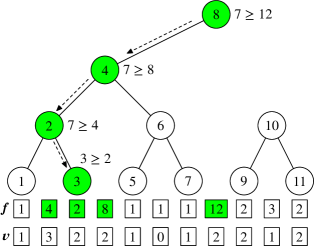
Figure 2: Pseudocode for find, and a sample execution on the tree of Figure 1: we are looking for the rightmost position with prefix sum at most $7$. We highlight the visited nodes and the associated elements in the vector $\bm{f}$ representing the tree. The test is against the element of $\bm{f}$ associated with the node. The returned pair is $\langle 3,1\rangle$.

The $\operatorname{\textsf{find}}_{\bm{f}}(x)$ operation is now simply a standard search on the sideways heap: we start at the root $\lambda n$, thus knowing the sum of the first $2^{\lambda n}$ values, and then move to the left or right child depending on whether $x$ is smaller or greater than that sum. Note that when we move to the left child $x$ remains unchanged, but when we move to the right child we have to subtract from $x$ the partial sum stored in the current node. Non-existing nodes are simply ignored (we follow their left child; see line 5 of Figure 2).

Fenwick shows that $\operatorname{\textsf{find}}_{\bm{f}}(x)=\operatorname{\textsf{find}}_{\bm{v}}(x)$. Figure 2 illustrates with an example the sequences of nodes traversed by a find operation.

4.2 The interrogation tree

To compute a prefix sum on $\bm{v}$ we use the interrogation tree. The tree has an implicit root $0$. The parent of node $j$ is

$$\operatorname{\textsf{int}}(j)=j-(1\mathbin{\ll}\rho j)=j\mathbin{\&}(j-1),$$

that is, $j$ with the lowest one cleared; note that the resulting tree is not a binary tree (in fact, the root has infinite degree). The primitive $\operatorname{\textsf{prefix}}_{\bm{f}}(j)$ accumulates partial sums on the path from node $j$ to the root (excluded), and Fenwick shows that $\operatorname{\textsf{prefix}}_{\bm{f}}(p)=\operatorname{\textsf{prefix}}_{\bm{v}}(p)$. Figure 3 illustrates with two examples the sequences of nodes traversed by a prefix operation.

Note that we use the same name for the abstract operation on the list and the implementation in a Fenwick tree to avoid excessive proliferation on names. The subscript should always make the distinction clear.

1:function $\mathrm{prefix}$($j$) 2:     $p\leftarrow 0$ 3:     while $j\neq 0$ do 4:         $p\leftarrow p+f[j]$ 5:         $j\leftarrow j\mathbin{\&}(j-1)$ 6:     end while 7:     return $p$ 8:end function

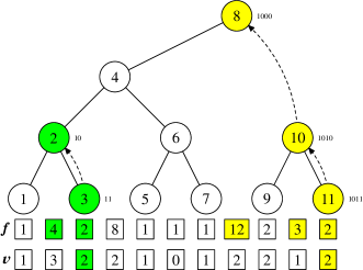
Figure 3: Pseudocode for prefix, and two sample executions on the tree of Figure 1: on the left the nodes traversed computing the sum of the first three elements, and on the right the nodes traversed computing the sum of the first eleven (i.e., all) elements. The value returned is the sum of the elements of $\bm{f}$ associated with the visited nodes. Note how the sequence of node indices is obtained by deleting the lowest bit set.

We remark that the interrogation tree can be also scanned in a top-down fashion, that is, from the root to the leaves. The sequence of values of $j$ that reaches the leaf $p$ starting from the root (i.e., $j=0$) is given by the rule

$$j\leftarrow j\mathbin{|}\bigl{(}1\ll\lambda(j\oplus p)\bigr{)}.$$

The rule adds to $j$ the bits sets in $p$ one by one, from the most significant one to the least significant one, thus selecting at each step the correct child.

4.3 The update tree

Finally, when modifying $v_{j}$ by adding the value $c$, Fenwick shows that we have to update $\bm{f}$ by adding $c$ to all nodes along a path going up from node $j$ in the update tree. In this tree, the parent of node $j$ is

$$\operatorname{\textsf{upd}}(j)=j+(1\mathbin{\ll}\rho j)=j+(j\mathbin{\&}-j).$$

If $j$ is an odd multiple of $2^{a}$, that is, $j=c2^{a}$ with $c$ odd, its parent is $(c+1)2^{a}$. We stop updating when the next node to update is beyond $n$. We call this operation $\operatorname{\textsf{add}}_{\bm{f}}(j,x)$. Figure 4 illustrates with two examples the sequences of nodes traversed by a add operation.

1:function $\mathrm{add}$($c,j$) 2:     while $j\leq n$ do 3:         $f[j]\leftarrow f[j]+c$ 4:         $j\leftarrow j+(j\mathbin{\&}-j)$ 5:     end while 6:end function

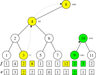
Figure 4: Pseudocode for add, and two sample executions on the tree of Figure 1: on the left the nodes traversed when updating the third element, and on the right the nodes traversed updating the ninth element. During the traversal, the argument $c$ is added to all elements of $\bm{f}$ associated with the visited nodes. Note how the sequence of node indices is obtained by adding the lowest bit set.

Note that technically the update tree is a forest, but for convenience and historical reasons we still refer to it as a tree. More precisely, as in the case of sideways heaps we could add implicit nodes $(n\,\mathpunct{\ldotp\ldotp}1\ll(\lambda n+1)]$ containing no partial sum which would make the forest into a tree.

It is easy to prove the following remarkable duality:

Proposition 1

$\operatorname{\textsf{int}}(-j)=-\operatorname{\textsf{upd}}(j)$.

Proof. Immediate, as $\rho j=\rho(-j)$ and $\operatorname{\textsf{int}}(-j)=(-j)-(1\ll\rho(-j))=-(j+(1\ll\rho j))=-\operatorname{\textsf{upd}}(j)$.  

The equation above can be used to provide a top-down scanning towards the leaf $p$, analogously to the case of int. The rule is simply

$$j\leftarrow-\bigl{(}-j\oplus(1\ll\lambda(-j\oplus-p))\bigr{)},$$

starting from $j=n\mathbin{\&}\bigl{(}-1\ll\lambda\bigl{(}n\oplus p\oplus(1\ll\rho p)\bigr{)}$, which in two’s complement arithmetic can be written as $n\mathbin{\&}(-1\ll\lambda\bigl{(}n\oplus(p\mathbin{\&}(p-1))\bigr{)}$. Alternatively, using the convention that $\lambda 0=-1$ and that negative shifts are shifts in the opposite direction one can express the starting node as $j=n\mathbin{\&}\bigl{(}-1\ll\lambda(n\oplus p)\bigr{)}$.

While apparently the top-down rule for upd requires many more operations, we can in fact perform the whole scan using negative indices: once the initial node has been set up in this way, the only difference between the two algorithms is that we have to remember to negate the result of the update rule to obtain the actual node of the tree.

4.4 Bounded lists and complemented find

Departing from the original definition, we will also assume the existence of an upper bound $B$ on the values in the list represented by the tree (i.e., $v_{i}\leq B$). Note that this is a not bound on the partial sums, as they are sums of such values, but it is easy to see that the upper bound for the partial sum of index $j$ will be $2^{\rho j}B$, so one needs $\bigl{\lceil}\lg\bigl{(}2^{\rho j}B+1\bigr{)}\bigr{\rceil}$ bits to store it.

Using the bound $B$, we now define an additional operation, complemented find, by

$$\overline{\operatorname{\textsf{find}}}_{\bm{v}}(x)=\max\bigl{\{}\mskip 1.5mup\mid pB-\operatorname{\textsf{prefix}}_{\bm{v}}(p)\leq x\mskip 1.5mu\bigr{\}}\qquad x\in\mathbf{N}.$$

This operation is not relevant when using a Fenwick tree to keep track of prefix sums, but will be essential to implement selection on zeros.

An implementation of complemented find is given in algorithm 1. Note that the only difference with a standard find (Figure 2) happens at 6: instead of considering the value of a node, we compute the difference with the maximum possible value stored at the node.

For both versions of find, we actually consider two return values: the length of the longest prefix with (complemented) sum less than or equal $x$, and the excess with respect to said (complemented) prefix sum. Once again, in the case the Fenwick tree is used just to keep track of prefix sums the excess is not particularly useful, but it will be fundamental in implementing selection primitives.

Algorithm 1 Complemented find for a Fenwick tree $\bm{f}$ with bound $B$.

1:function $\overline{\mathrm{find}}$($k$)

2:     $p\leftarrow 0$

3:     $q\leftarrow 1\mathbin{\ll}\lambda n$

4:     while $q\neq 0$ do

5:         if $p+q\leq n$ then

6:              $m\leftarrow B2^{\rho(p+q)}-f[p+q]$

7:              if $k\geq m$ then

8:                  $p\leftarrow p+q$

9:                  $k\leftarrow k-m$

10:              end if

11:         end if

12:         $q\leftarrow q\mathbin{\gg}1$

13:     end while

14:     return $\langle p,k\rangle$

15:end function

5 Compression and layout

Recent computer hardware features a growing performance gap between processor and memory speed. Keeping most of the computation into the cache can increase significantly the performance of data structure. Thus, compressed, compact or succinct data structures may require more complex operation for queries and updates, but, at the same time, by storing information more compactly they make it possible to increase performance by using the cache more efficiently.

We have explored several different forms of compression in order to balance the trade-off between the time required to retrieve uncompressed information and the time required to access to such data from the physical memory. After an experimental analysis we are reporting here the two most relevant ones.

5.1 Bit compression

As we explained in Section 4, we assume to have a bound $B$ on the values $v_{i}$ represented by the tree; let $S=\lceil\lg(B+1)\rceil$. In our implementation, we use $S$ bits for the leaves, $S+1$ bits for the nodes at level one, and so on. In general, we use $S+\rho j$ bits to store the partial sum at node $j$ (which is slightly redundant, in particular when $B$ is a power of two).

Figure 5: The bit-compressed Fenwick layout. Each box contains the index $j$ of the associated node, and the width in bits of each box is $S+\rho j$.

To be able to fully exploit bit compression, we need to lay out all partial sums consecutively in a bit array: an example is shown in Figure 5. A useful fact is that if we assume we can compute in constant time sideways sums, then we can compute in constant time the sum of the bit sizes of the first $j$ partial sums.

Proposition 2

For $0\leq j\leq n$ we have

$$\sum_{i=1}^{j}\bigl{(}S+\rho i)=j\cdot(S+1)-\nu j.$$

Proof. The only part that needs proof is $\sum_{i=1}^{j}\rho i=j-\nu j$, which is noted by Knuth. [11, 7.1.3]  

Note that the number of possible configurations of the tree is $(B+1)^{n}$, so the information-theoretical lower bound to store the tree is $\lceil n\lg(B+1)\rceil$ bits. Adding up on all nodes, similarly to Proposition 2 we obtain

$$\sum_{i=1}^{n}(S+\rho i)=nS+n-\nu n<n(1+S)=n(1+\lceil\lg(B+1)\rceil)\leq 2n\lg(B+1)\leq 2\lceil n\lg(B+1)\rceil.$$

Thus, our bit-compressed Fenwick tree qualifies as a compact data structure—one that uses space that is a constant number of times the information-theoretical lower bound.

For $B=1$ and $n$ a power of two our bound is tight, but for larger values of $B$ it is rather rough: for example, when $B=63$ we use less than $7n$ bits, whereas the information-theoretical lower bound is $6n$. In fact, for $B>3$ a better bound is

$$\sum_{i=1}^{n}(S+\rho i)\leq n(1+\lceil\lg(B+1)\rceil)\leq 2n+\lceil n\lg(B+1)\rceil,$$

which shows that we are actually losing at most two bits per element with respect to the lower bound; this bound is tight when $B$ is a sufficiently large power of $2$.

5.1.1 Byte compression

Another possibility, trading (in principle) space for speed, is to round up the size of each node to its closer byte. In this setting, the partial sum for node $j$ requires $\bigl{\lceil}\bigl{(}\rho j+S\bigr{)}/8\bigr{\rceil}$ bytes and starts at byte

$$\sum_{k=1}^{w/8}i\left\lceil\frac{S}{8k}\right\rceil.$$

The main problem of this approach is that we cannot provide a closed-form formula like that given in Proposition 2. To compute the starting byte of node $j$ we need to establish how many nodes using at least $k$ bytes appear before $j$.

To overcome this issue, we suggest an even looser compression strategy: instead of rounding up the space required by each node to the next byte, one can use just three byte sizes for partial sums: $\left\lceil(\lg(B+1))/8\right\rceil$, $\left\lceil(\lg(B+1))/8\right\rceil+1$ or full size (no compression). Let $b=\left\lceil(\lg(B+1))/8\right\rceil$ and let $d=8b-\lceil\lg(B+1)\rceil$; the sum of the byte size of the first $j$ partial sums is

$$\overbrace{jb}^{\text{at least $b$ bytes for each node}}+\overbrace{(j\mathbin{\gg}d)}^{\text{nodes with at least one additional byte}}+\overbrace{\left(j\mathbin{\gg}(d+8)\right)\cdot(w/8-b+1).}^{\text{uncompressed nodes multiplied by their additional space}}$$ (3)

In this way, one provides a byte-sized optimal compression for the lower nodes of the tree, and leave uncompressed everything above. This simplification has practically no impact on the overall space used by the Fenwick tree, as just a very small fraction of nodes will be represented in uncompressed form. For example, even in trees with height $64$ (the worst-case scenario if you want to store each node in a single word of a $64$-bit processor) only about the $0.026\%$ of the nodes reside in the third (uncompressed) partial sum.

As we will see in our experimental analysis, this looser byte compression mechanism happens to offer often faster access to the partial sums than the bit compression scheme.

5.2 The level-order layout

Compression is not the only way to improve cache efficiency. Another important aspect is prefetching: instead of fetching the data when it is needed, a prefetcher works by guessing what the next requested data will be and fetching it in advance. If the prefetching succeeds—that is, if the fetched data will be actually used in the near future—a cache miss is prevented and the execution will be faster. If the prefetcher makes the wrong guess, however, a cache line will be replaced with useless information and the prefetching might cause additional cache misses. Both hardware and software prefetchers exists, and the key to take advantage of their capabilities is to dispose the data in a way that the accesses made by the most frequent operations follow a simple and well defined pattern.

To find a predecessor, the Fenwick tree needs in the worst case (and also in the average case) to query the value of a logarithmic number of nodes. At each step, one of the children of the current node will be selected to continue the search, and the distance between two children of a node of height $h$ is $2^{h-1}$: one of the children, and we cannot predict which, will be reached in the next iteration. For $h$ enough large so that the two children lie in different cache lines the prefetcher can either make a guess and succeed with a probability of $1/2$, or it can prefetch both of them, wasting a cache line and doubling the required number of memory accesses.

To help cache prefetchers in making the correct guess every time we might modify the layout of the partial sums, and proceed in level order: first the root, then the children of the root, and so on. At that point, each pair of children would be at distance one, and thus much likely on the same cache line.

Of course this change of disposition does not come for free. If we lay out the levels in a single array, with pointers locating the start of each level, it will become very difficult to increase the number of nodes of the tree: this solution is thus restricted to Fenwick trees with immutable size. The alternative is to add a level of indirection, and thus to have an array of pointers, each to a different level. As a small advantage, since each level is compressed in the same way, once we locate the start of a level it is easier to find a node than in the case of a Fenwick layout.

We will use always such an implementation; as a consequence, every node in the level-order layout will be identified by two integers: its level $\ell$ and its zero-based index $k$ in its level. Nodes with $\ell=0$ are the leaves. This representation and the classic Fenwick representation are connected by the following easily proved proposition:

Proposition 3

A node with index $j$ in the classical Fenwick layout has level $\rho j$ and index $j\mathbin{\gg}(1+\rho j)$ in the level-order layout. A node with level $\ell$ and index $k$ in the level-order layout has index $(2k+1)\ll\ell$ in the classical Fenwick layout.

This bijection induces parent-children relationship on the level-order layout: in particular, it is easy to show that:

• for $\ell>0$, the children of node $\langle\ell,k\rangle$ in the sideways heap are $\langle\ell-1,2k\rangle$ and $\langle\ell-1,2k+1\rangle$ (but note that the second child might not exist);

• for $0<k\leq n\mathbin{\gg}(\ell+1)$, the parent of node $\langle\ell,k\rangle$ in the interrogation tree is $\langle\ell+1+\rho k,k\mathbin{\gg}(1+\rho k)\rangle$;

• for $0\leq k<n\mathbin{\gg}(\ell+1)$, the parent of node $\langle\ell,k\rangle$ in the update tree is $\bigl{\langle}\ell+1+\rho\bar{k},k\mathbin{\gg}\bigl{(}1+\rho\bar{k}\bigr{)}\bigr{\rangle}$.

6 Alignment problems

The Fenwick tree in Fenwick layout is extremely sensitive to the alignment of the partial sums. In our experiments, alignment problems can cause a severe underperformance of the primitives, which can be up to three times slower in the case of the bit-compressed tree.

6.1 Misalignment

To understand why this can happen, consider a standard technique for reading a sequence of bits which starts at position $p$ when $p$ is not byte-aligned (i.e., a multiple of eight): one uses an unaligned word read at byte position $\lfloor p/8\rfloor$, and then one suitably shifts and masks the result (note, however, that this method does not allow in general to read bit blocks of length close to $w$, as they might span multiple words).

Consider now a bit-compressed tree of $n$ nodes, with $n$ larger than the size $M$ of a memory page in bits, which we assume to be a power of two. As it is easy to see from the nature of the parent-child relationship of the three implicit trees described in Section 4, in all operations the partial sums whose indices have a large number of trailing zeros in binary representation (i.e., $\rho j$ is large, where $j$ is the index) are the ones more frequently accessed.

Let as assume that the memory containing the partial sums is aligned with a memory page (e.g., if mmap() is used to allocate memory), and let us look at the bit position in memory of the partial sum of index $1\ll\lambda n$. Using Proposition 2 it is immediate to see that it will be

$$(1\ll\lambda n)\cdot(S+1)-1-S-\rho(1\ll\lambda n).$$

Thus, if $S+1+\rho(1\ll\lambda n)=S+1+\lambda n\leq w-8$, reading the partial sum as above will cause a word read across memory pages, which will access to two distinct memory pages and usually generate two cache misses.

Figure 6: An example of misalignment: rectangles are word-aligned words, and $j(S+1)$ is on the border of a memory page. By Proposition 2 the partial sum of node $j$ is stored in the highlighted block of $S+\rho j$ bits starting at $j(S+1)-\nu j-(S+\rho j)$, but using unaligned reads we would actually access the $w$ bits indicated by the double arrow, thus accessing two distinct memory pages. Due to the layout of the Fenwick tree, these kind of reads are very frequent.

As shown in Figure 6, the same argument applies to any node whose index $j$ is such that $2^{\rho j}$ is a multiple of $M$ (so the partial sum is stored at the very end of a memory page) and $1+S+\rho j\leq w-8$ (so we read an across-page word). As we mentioned, this high number of across-page read/write operation can slow down the data structure by a factor of three, because it affects the nodes that are accessed more frequently.

To work around this problem, we note the following property:

Proposition 4

If $j\cdot(S+1)$ is a multiple of $w$, and the memory representation of the tree is shifted by one bit to the right, the partial sum of index $j$ is contained in a word-aligned word.

Proof. Due to the one-bit shift, the partial sum of index $j$ will start at position $j\cdot(S+1)-\nu j-(S+\rho j)+1$ (included) and end at position $j\cdot(S+1)-\nu j+1$ (excluded). However,

$$\nu j+\rho j\leq\lambda j+1\quad\text{for $1\leq j\leq n$,}$$

because $\nu j$ is the number of ones in the binary representation of $j$, whereas $\rho j$ is bounded by the number of zeros, so

$$\nu j-1+S+\rho j\leq S+\lambda j\leq w,$$

because the largest size in bits of a partial sum cannot exceed $w$. Thus, the partial sum of index $j$ is contained in the word of (zero-based) index $j\cdot(S+1)/w-1$.  

As a consequence, we can read frequently accessed partial sums (which have a large $\rho j$, so $j\cdot(S+1)$ is a multiple of $w$) using word-aligned words (i.e., if the partial sum starts at position $p$, we read the word of index $\lfloor p/w\rfloor$ and then suitably shift and mask). The proposition will work also when $j\cdot(S+1)$ is a multiple of eight, albeit the word containing the partial sum will be just byte-aligned. When $j\cdot(S+1)$ is not a multiple of eight, if we want to guarantee that a single word access will retrieve correctly the partial sum we have to make some assumption: in particular, the largest partial sums we might read, which will be made of $S+2$ bits (as $\rho j<3$), must be at most $w-7$ bits long, that is, $S\leq w-9$. In practice, on $64$-bit architectures we have to require $S\leq 55$, that is, $B<2^{55}-1$, which is more than sufficient for our purposes. Alternatively, one has to resort to read one or two word-aligned words and reconstruct the partial sum from those.

Note that this bound is tight: if $w=64$, $S=56$ and $j=60$ the last bit of the associated $58$-bit partial sum will be in position $3480$, so the partial sum will span two words.

We remark that the byte-compressed Fenwick tree in Fenwick layout has no across-page access problems, as all partial sums are byte-aligned, and if $\rho j$ is large enough all three summands of the offset formula (3) are multiples of $w$.

6.2 Hyper-alignment

The second alignment problem, which is more subtle and affects even the classical version, is that frequently accessed partial sums are stored at memory locations with the same residual modulo $2^{a}w$, for small $a$. This is obvious in the classical construction, as frequently accessed partial sums have indices with a large $\rho j$. In the bit-compressed tree, instead, this pattern is due to access being modeled using Proposition 4. This kind of hyper-aligned access implies that all the nodes end up being cached in the same way of the cache, as multi-way caches usually decide in which way to store a cache line using the lowest bits of the address.

The solution we adopt is that of perturbing slightly the data structure so to spread the residuals of the memory addresses of frequently accessed partial sums across the whole possible range of values. To obtain this result, we insert $w$-bit sized holes at regular intervals. By making the intervals a sufficiently large power of two, the impact on space usage is negligible, and computing the actual position requires just an additional shift and a sum. By making the holes $w$-bit wide, all the good alignment properties of the structure (i.e., Proposition 4) are preserved. The find operations are the one more affected: a standard Fenwick tree on a large list (i.e., 100M elements) features 30% shorter execution times on our hardware once holes are put in place.

7 Ranking and selection

Let us now get back to problem of dynamic rank and selection. Consider a dynamic bit vector $\bm{b}$: that is, we are able to change the value of $b_{i}$ (set and clear operations) and expand or reduce the length of $\bm{b}$ ($\operatorname{\textsf{push}}$ and $\operatorname{\textsf{pop}}$ operations).

If the vector is very short, it is possible to perform ranking and selection very quickly using broadword programming. Modern computers are capable of computing sideways additions on a word using a single instruction, usually called popcount (population count). With this instruction we can easily perform ranking within a word after suitably masking. Also selection in a word can be performed quickly,[15, 4] particular on very recent Intel architectures which provide the PDEP instruction. In practice, since sequential memory accesses are highly amenable to cache prefetching, a linear search is still the fastest way to perform dynamic ranking and selection on a sufficiently small bit vector.

For larger vectors, we can split the problem into ranking and selection over blocks of $q$ bits, where a linear scan is sufficiently fast, and keeping track of the prefix sums of the number of ones in each block using a Fenwick tree $\bm{f}$. At that point, we can implement rank and select as

$$\operatorname{\textsf{rank}}_{\bm{b}}(p) =\operatorname{\textsf{prefix}}_{\bm{f}}(m)+\operatorname{\textsf{rank}}_{\bm{b}[mq\,\mathpunct{\ldotp\ldotp}(m+1)q)}(p\bmod q) m=\lfloor p/q\rfloor$$ where

$$\operatorname{\textsf{select}}_{\bm{b}}(k) =pq+\operatorname{\textsf{select}}_{\bm{b}[mq\,\mathpunct{\ldotp\ldotp}(m+1)q)}(g) \langle p,g\rangle=\operatorname{\textsf{find}}_{\bm{f}}(k) m=\lfloor p/q\rfloor$$ where and

Note that this strategy allows us to compute rank and select queries on zeros too. Select on zeroes consists in replacing $\operatorname{\textsf{find}}$ with $\overline{\operatorname{\textsf{find}}}$ and flipping all the bits during linear scans: the bound $B$ of Section 4.4 is $q$. Rank on zeros is simply $p-\operatorname{\textsf{rank}}_{\bm{b}}(p)$.

We have previously assumed we are capable of computing ranking and selection within a word using some extremely fast operations, such as dedicated assembly instruction. This assumption suggests the choice of a fairly large $q$, as the bigger is $q$, the smaller will be additional space required to store the Fenwick tree. However, many RISC architectures such as the widespread ARM are not capable of performing these operations in few clock cycles. In this case, the compact structures described in this paper might be even more relevant, as a small $q$ implies a larger tree.

8 Experiments

In this section we present the results of our experiments, which were performed on an Intel® Core™ i7-7770 CPU @3.60GHz (Kaby Lake), with 64 GiB of RAM, Linux 4.17.19 and the GNU C compiler 8.1.1. We use transparent huge pages, a relatively new feature of the operating system that makes available virtual memory pages of $2$ MiB, which significantly reduce the cost of accessing the TLB (Translation Lookaside Buffer) for large-scale data structures.

We will present two sets of experiments:

• In the first set, we examine the primitives of the Fenwick tree in isolation, exploring the effects of layout and compression policies on speed. We generate list of values chosen uniformly at random, and average the running time of a large number of queries at random locations. Note that both $\operatorname{\textsf{prefix}}$ and $\operatorname{\textsf{add}}$ are data-agnostic, in the sense that the execution flow does not depend on the content of the tree; the execution flow of $\operatorname{\textsf{find}}$, on the contrary, depends on the content.

• In the second set, we use a Fenwick tree to support rank and selection: in this case, beside the way we structure the tree we also explore the effect of different block sizes; as a baseline, we report results for Nicola Prezza’s library for dynamic bit vectors [13], which is the only practical available implementation we are aware of. We generate random bit vectors with approximately the same number of ones and zeroes, and, again, average the running time of a large number of queries at random locations.

In both cases, we take care of potential dead-code elimination by assigning the value returned by each test to a variable which is in the end assigned a volatile dummy variable. Moreover, to avoid excessive and unrealistic speculative execution, in a sequence of calls to a primitive we xor the next argument using the lowest bit of the previously returned value, as this approach creates a chain of dependencies among successive calls.

We do not report the results for complemented find and since both its algorithm and its memory-access pattern are very similar to that of a standard find, so their performances are very similar. The same argument holds for ranking and selection on zeros.

Finally, we report results in two real-world applications: counting the number of transpositions generating a permutation, and generating pseudorandom graphs following a preferential attachment model.

8.1 Variants

Name	Comment
bit$[\ell]$	Level-order layout; bit compression
byte$[\ell]$	Level-order layout; byte compression
fixed$[\ell]$	Level-order layout; fixed-width representation
bit$[F]$	Classical Fenwick layout; bit compression
byte$[F]$	Classical Fenwick layout; byte compression
fixed$[F]$	Classical Fenwick layout; fixed-width representation

Table 1: Naming scheme for the Fenwick trees appearing in experiments. Implementations of dynamic bit vectors have an additional number denoting the size of a block in word (i.e., bits$[\ell]8$).

We consider a number of implementations displayed in Table 1. We use three different kinds of compression strategies, namely: no compression (dedicating $64$ bits for each node), byte compression (see Section 5.1.1) and bit compression (see Section 5.1). For each of them we consider the classical and level-order layout. Since we want to use the results of this benchmark as a reference for choosing good parameters for the rank and selection structures, we are fixing to $64$ the bound $B$ on the leaves.

We remark that throughout our graphs a few spikes are visible: they are due to the nonlinear behavior of the tree, as when the size reaches a power of two a new root is created, usually in a new memory page if the tree is page-aligned, and the tree becomes as unbalanced as possible (e.g., updating an element will require one additional iteration). This fact can increase the number of TLB/cache misses and the number of average accesses: as the number nodes grow, this cost is amortized.

8.2 Fenwick trees

Figures 7-9 report the performance of several variants for the $\operatorname{\textsf{prefix}}$, $\operatorname{\textsf{find}}$ and $\operatorname{\textsf{add}}$ operations. Note that we do not report data about $\operatorname{\textsf{push}}$/$\operatorname{\textsf{pop}}$, but a $\operatorname{\textsf{pop}}$ primitive would be constant-time (just update the size of the tree, as indices of parents in the update tree are always larger than indices of their children), while the performance of the $\operatorname{\textsf{push}}$ primitive is essentially identical to that of $\operatorname{\textsf{add}}$ (we will, however, give a sample application using $\operatorname{\textsf{push}}$).

• In the performance of $\operatorname{\textsf{prefix}}$, it is immediate evident the point in which each structure goes out of the L3 cache. Non-compressed structures have a slight advantage initially, but they are almost twice as slow when the compressed structures still fits in cache. After all structure go out of the cache, the advantage of the simpler code of non-compressed structure shows again, albeit the speedup is very marginal compared to the byte-compressed structures. The bit-compressed structure have significantly more complex code, and in particular a test that decides whether to align access to bytes or words, and this cost increases logarithmically.

• The graphs of $\operatorname{\textsf{find}}$ are somehow smoother, due to the more regular cache usage. What is evident here is the bad performance of the classical Fenwick tree, and that the fastest structure (except for very small scale) is the level-order byte-compressed version. Note that a $\operatorname{\textsf{find}}$ operation requires always $\lg n$ accesses, whereas in the other cases, as noted by Fenwick [3], assuming a perfect sideways heap only $(1+\lg n)/2$ are required on average.

• The graphs for $\operatorname{\textsf{add}}$ show a behavior similar to that of $\operatorname{\textsf{prefix}}$, but with less pronounced differences in performance. In particular, the Fenwick and the level-order performances are much closer.

Note that the advantage of compressed trees in underestimated by our benchmarks, as the cache will be shared with other parts of the code. Benchmarking different kind of trees inside a specific application is the most reliable way to determine which variant is the most efficient for the application at hand.

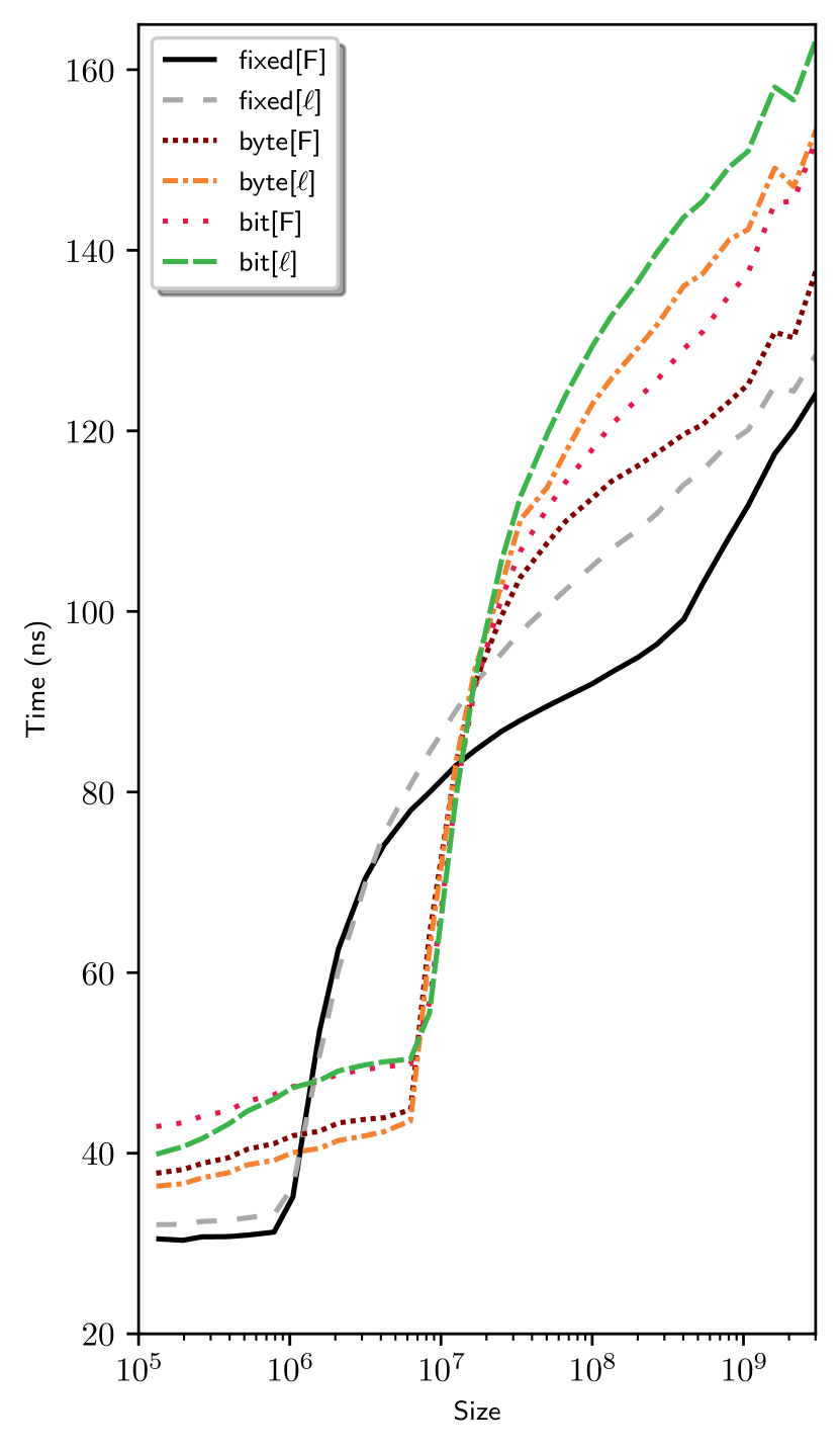
Figure 7: Performance of $\operatorname{\textsf{prefix}}$.

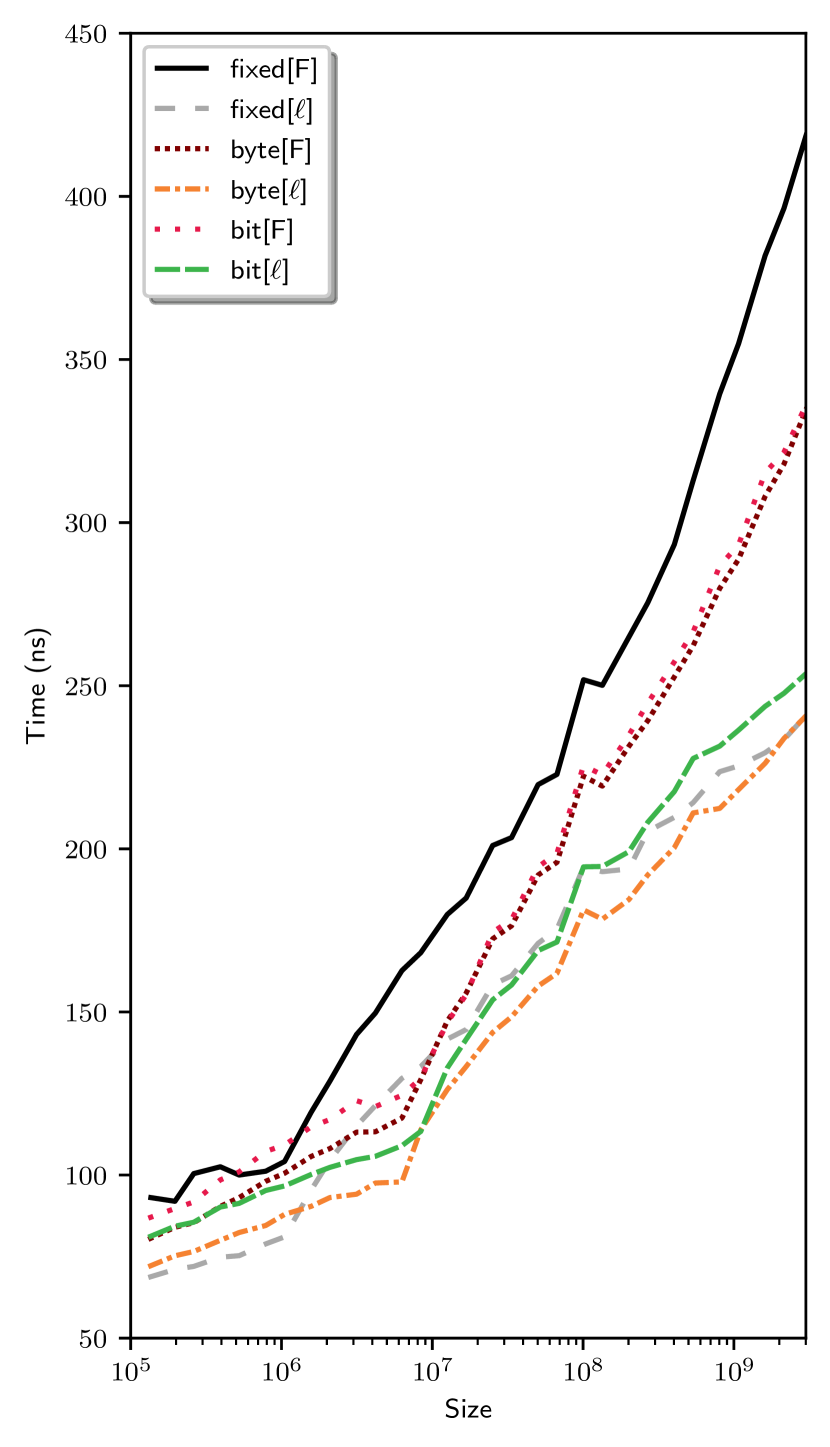
Figure 8: Performance of $\operatorname{\textsf{find}}$.

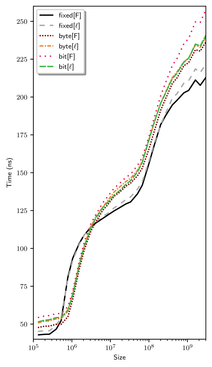
Figure 9: Performance of $\operatorname{\textsf{add}}$.

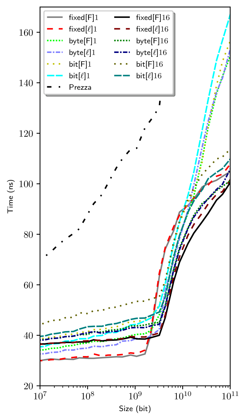
Figure 10: Performance of $\operatorname{\textsf{rank}}$.

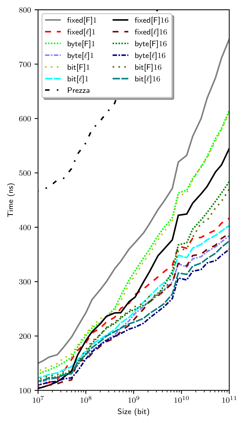
Figure 11: Performance of $\operatorname{\textsf{select}}$.

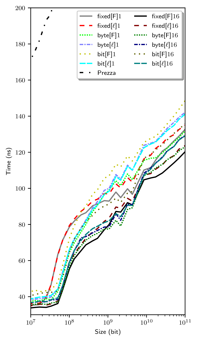
Figure 12: Performance of bit updates.

8.3 Dynamic bit vectors

The graphs for operations on dynamic bit vectors, show in Figures 10-12, are somewhat smoother than those for the Fenwick trees, because of the much smaller size (a small fraction of the size of the bit vector). We report experiment with trivial, one-word blocks, and with blocks make of $16$ words. Table 3 reports a space-time tradeoff plot for the same variants at three different sizes. We did not implement a $\operatorname{\textsf{push}}$/$\operatorname{\textsf{pop}}$ primitive, as its performance would be essentially constant-time, in case the underlying Fenwick tree does not change, or identical to $\operatorname{\textsf{push}}$/$\operatorname{\textsf{pop}}$ operations on the tree. For these experiments we are comparing the performance of our implementations with Prezza’s library for dynamic bit vectors.

• When ranking, one-word blocks have a very small advantage at small size (about $5$ ns), due to the simpler code, but the performance penalty on large bit vector is very significant. The performance of the underlying Fenwick tree follows closely the results for $\operatorname{\textsf{prefix}}$.

• When selecting, lever-order trees with byte and bit compression are the fastest. In this case, blocks reduce significantly the number of level of the tree, bringing bit compression close to the performance of byte compression.

• Updates are the only operation in which fixed-width Fenwick trees win, albeit by a very small margin, on the corresponding byte-compressed variant.

Table 2 reports the space usage per bit. With one-word blocks, a fixed-size Fenwick tree uses the same space of the bit vector, increasing space usage twofold. Bit or byte compression bring down the space increase to $12$% and $16$%, respectively. With 16-word blocks, any Fenwick tree requires a space that is only a few percent of the bit vector. Prezza’s implementation uses $13$% additional space.

	fixed/1	byte/1	bit/1	fixed/16	byte/16	bit/16	Prezza
bits	$2.00$	$1.16$	$1.12$	$1.06$	$1.02$	$1.01$	$1.13$

Table 2: Average space used per bit on a $10^{9}$ bit vector. In our case, space depends on the block size and on the compression type. Prezza’s data structure average space is claimed to be around $1.2n$ bits [13], but we are reporting a better result obtained by inserting every element at the end (as it would happen in our case).

rank (ns)
select (ns)
update (ns)
	$10^{9}$ bits	$10^{10}$ bits	$10^{11}$ bits

Table 3: Space-time tradeoff plots for the dynamic bit vector implementations of Figure 10-12 at different sizes.

8.4 Counting transpositions

In this application, we use our data structures in a classical task: given a permutation $\pi$, count the number of transposition (e.g., exchanges of two elements) that are necessary to generate $\pi$. This computation is a fundamental step in computing Kemeny’s distance [9] (the number of transpositions that are necessary to transform a permutation in another), Kendall’s $\tau$ [10] (a statistical correlation index), etc. One starts from a permutation $\pi$ on $n$ elements, computes the inverse $\pi^{-1}$, initializes a bit vector containing $n$ ones, and then scans $\pi^{-1}$ (seen as a list of numbers): for each element $x$, one computes the rank at $x$, and then clears the bit of index $x$. In this way, every rank represents the number of elements that $x$ would be exchanged with in a bubble sort of $\pi$; the sum of these ranks is exactly the number of transposition generating $\pi$.

In Figure 13, we report the time per element to count transpositions using a standard Fenwick tree, as it happens in SciPy’s code, [8] using Prezza’s library and using a fixed-size and a byte-compressed implementation of our dynamic ranking structure. To maximize the difference between each structure, we generated $\pi^{-1}$ implicitly using a suitable linear congruential pseudorandom number generator with power-of-two modulus Besides the evident speed increase, our structures (and Prezza’s) are more than fifty times smaller than SciPy’s.

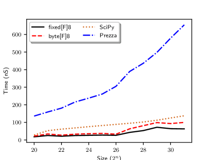
Figure 13: Counting transpositions of a random permutation. Note that the SciPy code uses more than fifty times more memory than the alternative structures.

8.5 Generating graphs by preferential attachment

A simple, classical model of random (undirected) graphs is the preferential attachment model: one fixes an integer $d$, a $d_{0}\geq d$, and starts with $d_{0}$ isolated vertices (with a self-loop). Then, at each iteration a vertex of degree $d$ is added to the graph, and connected to $d$ vertices chosen among the ones already generated in a way that is proportional to their degree. If enough memory is available, a simple way to sample vertices proportionally to the degree is to maintain a list of vertices in which each vertex is repeated as many times as its degree, and then just sample from the list. For large graphs, however, the list becomes unmanageable.

The Fenwick tree offers a simple solution: one maintains a tree representing a list $\bm{v}$ containing the degree of each vertex, and at that point a find operation on a uniform random sample in the integer interval $[0\,\mathpunct{\ldotp\ldotp}2m)$, where $m$ is the current number of edges of the graph, samples vertices proportionally to their degree. Thus, we alternate find operations, to find vertices with which to connect, add operations, to update their degree, and $\operatorname{\textsf{push}}$ operations, one for each new vertex.

In Figure 14, we report the time necessary to generate a graph of a million vertices using four variants of our data structures for increasing $d$. The level-order layout is a clear winner, as predicted by the better cache behavior of $\operatorname{\textsf{find}}$. Note that the byte-compressed version is slower of the fixed-size version, but it uses much less memory, as $B=dn$. This fact is apparently in contradiction with Figure 8: however, in the sampling process the nodes traversed by find operations are strongly biased towards nodes that lead to vertices of high degree, so the advantage of the simpler code of the fixed-size version outweighs its larger memory footprint.

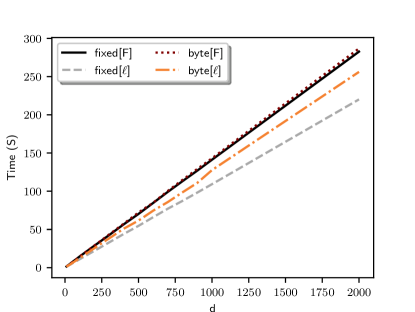
Figure 14: Generating preferential-attachment pseudorandom graphs with a million vertices and average degree $d$ using Fenwick trees. Level-order layout has a clear advantage.

9 Conclusions

We have presented improved, cache-friendly and prediction-friendly variants of the classical Fenwick tree. Besides maintaining a prefix-sum data structure, the tree can be used to provide an efficient dynamic bit vector with selection and ranking with a very small space overhead, albeit size can be changed only by adding or removing a bit at the end, rather than at an arbitrary position.

The first takeaway lesson from our study is that it is fundamental to perturb the structure of a Fenwick tree in classical Fenwick layout so that it does not interfere with the inner working of multi-way caches: while this phenomenon has never been reported before, the interference can lead to a severe underperformance of the data structure.

The second lesson is that, in spite of its elegance, the Fenwick layout is advantageous only if the $\operatorname{\textsf{find}}$ primitive is never used (e.g., when counting transpositions). In all other cases, a level-order layout is preferable.

Bit-compressed versions are extremely tight, but the higher access time makes them palatable only when memory is really scarce: otherwise, byte-compressed versions provide often similar occupancy, but a much faster access. In particular, the faster $\operatorname{\textsf{find}}$ results we report are for a byte-compressed, level-ordered tree.

For what matter dynamic bit vectors, for the sizes we consider the best solution is a block large as one or two cache lines; the consideration made for Fenwick order vs. level order and compression are valid also in this case.

Albeit not reported in the paper, we also experimented with the idea of hybrid trees, which upper levels are level ordered, but lower lever have a Fenwick layout. In some architectures, and in particular if only small memory pages are available, they offer a performance that is intermediate between that of Fenwick layout and level-order layout. In general, for the upper levels one can always use a fixed-width Fenwick tree, as the number of nodes involved is very small, whereas lower levels benefit from compression.

Finally, we remark once again that due to the highly nonlinear effect of cache architecture, and to conflicting cache usage, benchmarking a target application with different variants is the best way to choose the variant that better suits the application.

References

- [1] Paul Beame and Faith E. Fich. Optimal bounds for the predecessor problem and related problems. Journal of Computer and System Sciences, 65(1):38–72, 2002.
- [2] Philip Bille, Anders Roy Christiansen, Nicola Prezza, and Frederik Rye Skjoldjensen. Succinct partial sums and fenwick trees. In Gabriele Fici, Marinella Sciortino, and Rossano Venturini, editors, String Processing and Information Retrieval, pages 91–96. Springer International Publishing, 2017.
- [3] Peter M. Fenwick. A new data structure for cumulative frequency tables. Software: Practice and Experience, 24(3):327–336, 1994.
- [4] Simon Gog and Matthias Petri. Optimized succinct data structures for massive data. Software: Practice and Experience, 44(11):1287–1314, 2014.
- [5] Dov Harel. Efficient Algorithms with Threaded Balanced Trees. PhD thesis, University of California at Irvine, 1980.
- [6] Wing-Kai Hon, Kunihiko Sadakane, and Wing-Kin Sung. Succinct data structures for searchable partial sums with optimal worst-case performance. Theoretical Computer Science, 412(39):5176–5186, 2011.
- [7] Guy Jacobson. Space-efficient static trees and graphs. In 30th Annual Symposium on Foundations of Computer Science (FOCS ’89), pages 549–554, Research Triangle Park, North Carolina, 1989. IEEE Computer Society Press.
- [8] Eric Jones, Travis Oliphant, Pearu Peterson, et al. SciPy: Open source scientific tools for Python, 2019.
- [9] John G. Kemeny. Mathematics without numbers. Daedalus, 88(4):577–591, 1959.
- [10] Maurice G. Kendall. A new measure of rank correlation. Biometrika, 30(1/2):81–93, 1938.
- [11] Donald E. Knuth. The Art of Computer Programming: Volume 4, Combinatorial algorithms. Part 1, volume 4A. Addison-Wesley, 2011.
- [12] Veli Mäkinen and Gonzalo Navarro. Dynamic entropy-compressed sequences and full-text indexes. ACM Trans. Algorithms, 4(3):32:1–32:38, 2008.
- [13] Nicola Prezza. A Framework of Dynamic Data Structures for String Processing. In Costas S. Iliopoulos, Solon P. Pissis, Simon J. Puglisi, and Rajeev Raman, editors, 16th International Symposium on Experimental Algorithms (SEA 2017), volume 75 of Leibniz International Proceedings in Informatics (LIPIcs), pages 11:1–11:15, Dagstuhl, Germany, 2017. Schloss Dagstuhl–Leibniz-Zentrum fuer Informatik.
- [14] Rajeev Raman, Venkatesh Raman, and S. Srinivasa Rao. Succinct dynamic data structures. In Frank Dehne, Jörg-Rüdiger Sack, and Roberto Tamassia, editors, Algorithms and Data Structures, number 2125 in Lecture Notes in Computer Science, pages 426–437. Springer Berlin Heidelberg, 2001.
- [15] Sebastiano Vigna. Broadword implementation of rank/select queries. In Catherine C. McGeoch, editor, Experimental Algorithms. 7th International Workshop, WEA 2008, number 5038 in Lecture Notes in Computer Science, pages 154–168. Springer–Verlag, 2008.