Optimizing Regularized Cholesky Score for Order-Based Learning of Bayesian Networks

Abstract

Bayesian networks are a class of popular graphical models that encode causal and conditional independence relations among variables by directed acyclic graphs (DAGs). We propose a novel structure learning method, annealing on regularized Cholesky score (ARCS), to search over topological sorts, or permutations of nodes, for a high-scoring Bayesian network. Our scoring function is derived from regularizing Gaussian DAG likelihood, and its optimization gives an alternative formulation of the sparse Cholesky factorization problem from a statistical viewpoint, which is of independent interest. We combine global simulated annealing over permutations with a fast proximal gradient algorithm, operating on triangular matrices of edge coefficients, to compute the score of any permutation. Combined, the two approaches allow us to quickly and effectively search over the space of DAGs without the need to verify the acyclicity constraint or to enumerate possible parent sets given a candidate topological sort. The annealing aspect of the optimization is able to consistently improve the accuracy of DAGs learned by local search algorithms. In addition, we develop several techniques to facilitate the structure learning, including pre-annealing data-driven tuning parameter selection and post-annealing constraint-based structure refinement. Through extensive numerical comparisons, we show that ARCS achieves substantial improvements over existing methods, demonstrating its great potential to learn Bayesian networks from both observational and experimental data.

1 Introduction

Bayesian networks (BNs) are a class of graphical models, whose structure is represented by a directed acyclic graph (DAG). They are commonly used to model causal networks and conditional independence relations among random variables. The past decades have seen many successful applications of Bayesian networks in computational biology, medical science, document classification, image processing, etc. As the relationships among variables in a BN are encoded in the underlying graph, various approaches have been put forward to estimate DAG structures from data. Constraint-based approaches, such as the PC algorithm [1], perform a set of conditional independence tests to detect the existence of edges. In score-based approaches, a network structure is identified by optimizing a score function [2, 3]. There are also hybrid approaches, such as the max-min hill-climbing algorithm [4], which use a constraint-based method to prune the search space, followed by a search for a high-scoring network structure.

The score-based search has been applied to three different search spaces: the DAG space [2, 5], the equivalence classes [6, 2] and the ordering space (or the space of topological sorts) [7, 8]. In this paper, we focus on the order-based search, which has two major advantages. First, the existence of an ordering among nodes guarantees a graph structure that satisfies the acyclicity constraint. Second, the space of orderings is significantly smaller than the space of DAGs or of the equivalence classes. Consequently, several lines of research have developed efficient order-based methods for DAG learning. Some methods adopt a greedy search in conjunction with various operators that propose moves in the ordering space [8, 9, 10, 11]. A greedy search, however, may easily be trapped in a local minimum, and thus different techniques were proposed to perform a more global search [12, 7, 13, 14]. In particular, stochastic optimization, such as the genetic algorithm [7, 15, 11] and Markov chain Monte Carlo [16, 17], has been advocated as a promising way to perform global search over the ordering space.

In spite of these methodological and algorithmic advances, there are a few difficulties in score-based learning of topological sorts for DAGs. First, the score of an ordering is usually defined by the score of the optimal DAG compatible with the ordering. The computational complexity of finding the optimal DAG given an ordering, typically by enumerating all possible parent sets for each node [18], can be as high as $O(p^{k+1})$ for $p$ nodes and a prespecified maximum indegree of $k$. Such computation is needed for every ordering evaluated by a search algorithm, which becomes prohibitive when $k$ is large. Second, although the ordering space is smaller than the graph space, optimization over orderings is still a hard combinatorial problem due to the NP-hard nature of structure learning of BNs [19]. It is not surprising that the performance of the above global optimization algorithms degrades severely for large graphs.

Motivated by these challenges, we develop a new order-based method for learning Gaussian DAGs by optimizing a regularized likelihood score. Representing an ordering by the corresponding permutation matrix $P$, the weighted adjacency matrix of a Gaussian DAG can be coded into a lower triangular matrix $L$. We add a concave penalty function to the likelihood to encourage sparsity in $L$, and thus achieve the goal of structure learning. Instead of a prespecified maximum indegree, which is ad hoc in nature, we provide a principled data-driven way to determine the tuning parameters for the penalty function. Finding the optimal DAG given $P$ is then reduced to $p$ decoupled penalized regression problems, which are solved by proximal gradient, an efficient first-order method, without enumerating possible parent sets for any node. Searching over $P$ is done by simulated annealing (SA). Other than using SA solely as a global optimization algorithm, we may also incorporate informative initial orderings, learned from an existing local algorithm, by setting a low starting temperature. Our numerical results demonstrate that this strategy substantially improves the accuracy of an estimated DAG. We note an interesting connection between our formulation and the sparse Cholesky factorization problem, and thus name our scoring function the regularized Cholesky score of orderings or permutations.

Regularizing likelihood with a continuous penalty function has been shown to be effective in learning Gaussian DAGs [20, 21]. These methods optimize a regularized likelihood score over the DAG space by blockwise coordinate descent, which is a local search algorithm in nature and thus likely to be trapped in a suboptimal structure. Using DAGs learned by these methods to generate initial orderings, our method can significantly improve the accuracy in structure learning. This highlights the advantages of combining local and global searches over the ordering space under an annealing framework. More recently, Champion et al. [15] developed a genetic algorithm that optimizes an $\ell_{1}$-penalized likelihood over a triangular coefficient matrix and a permutation to learn Gaussian BNs. However, the $\ell_{1}$ penalty tends to introduce more bias in estimation than a concave penalty, thus producing less accurate DAGs. The authors did not provide a principled method to select the tuning parameter for the $\ell_{1}$ penalty. Given a permutation, they optimize the network structure by an adaption of the least angle regression [22], which is closely related to the Lasso. In contrast, we use a more general and effective first-order method, the proximal gradient algorithm, which is applicable to many regularizers, including the $\ell_{1}$ and concave penalties. As shown by our numerical experiments, our method substantially outperforms their genetic algorithm.

The paper is organized as follows. Section 2 covers some background on Gaussian BNs and the role of permutations in identifying the underlying DAGs. We introduce the regularized Cholesky loss and set up the global optimization problem for BN learning in Section 3. In Section 4, we develop the annealing on regularized Cholesky score (ARCS) algorithm which combines global annealing to search over the permutation space and a proximal gradient algorithm to optimize the network structure given an ordering. We also propose a constraint-based approach to prune the estimated network structure after annealing process and a data-driven model selection technique to choose tuning parameters for the penalty function. Section 5 consists of exhaustive numerical experiments, where we compare our method to existing ones using both observational and experimental data. We conclude with a discussion in Section 6. All proofs are relegated to the Appendix.

2 Background

We start with some background on Bayesian networks. A Bayesian network for a set of variables $\{X_{1},\ldots,X_{p}\}$ consists of 1) a directed acyclic graph $\mathcal{G}$ that encodes a set of conditional independence assertions among the variables, and 2) a set of local probability distributions associated with each variable. It can be considered as a recipe for factorizing a joint distribution of $\{X_{1},\ldots,X_{p}\}$ with probability density

$$p(x_{1},\ldots,x_{p})=\prod_{j=1}^{p}p(x_{j}\mid\Pi_{j}^{\mathcal{G}}=pa_{j}),$$ (1)

where $\Pi_{j}^{\mathcal{G}}\subseteq\{X_{1},\ldots,X_{p}\}\setminus\{X_{j}\}$ is the parent set of variable $X_{j}$ in $\mathcal{G}$ and $pa_{j}$ its value. The DAG $\mathcal{G}$ is denoted by $\mathcal{G}=(V,E)$, where $V=\{1,\ldots,p\}$ is the vertex set corresponding to the set of random variables and $E=\{(i,j):i\in\Pi_{j}^{\mathcal{G}}\}\subseteq V\times V$ is the edge set. We use variable $X_{j}$ and node $j$ exchangeably throughout the paper. DAGs contain no directed cycles, making the joint distribution in (1) well-defined.

2.1 Gaussian Bayesian networks

In this paper, we focus on Gaussian BNs that can be equivalently represented by a set of linear structural equation models (SEMs):

$$X_{j}=\sum_{i\in\Pi_{j}^{\mathcal{G}}}\beta_{ij}^{0}X_{i}+\varepsilon_{j},\quad j=1,\ldots,p,$$ (2)

where $\varepsilon_{j}\sim\mathcal{N}(0,(\omega_{j}^{0})^{2})$ are mutually independent and independent of $\{X_{i}:i\in\Pi_{j}^{\mathcal{G}}\}$. Defining $B_{0}:=(\beta_{ij}^{0})\in\mathbb{R}^{p\times p}$, $\varepsilon:=(\varepsilon_{1},\ldots,\varepsilon_{p})^{\top}\in\mathbb{R}^{p}$, and $X:=(X_{1},\ldots,X_{p})^{\top}\in\mathbb{R}^{p}$, we rewrite (2) as

$$X=B_{0}^{\top}X+\varepsilon.$$ (3)

The model has two parameters: 1) $B_{0}$ as a coefficient matrix, sometimes called the weighted adjacency matrix, where ${\beta_{ij}^{0}}$ specifies a weight associated with the edge $i\to j$ and ${\beta_{ij}^{0}}=0$ for $i\notin\Pi_{j}^{\mathcal{G}}$, and 2) $\Omega_{0}:=\operatorname{diag}((\omega_{j}^{0})^{2})$ as a noise variance matrix. The SEMs in (2) define a joint Gaussian distribution, $X\sim\mathcal{N}(0,\Sigma_{0}),$ where $\Sigma_{0}$ is positive definite and given by

$$\Sigma_{0}^{-1}=(I-B_{0})\Omega_{0}^{-1}(I-B_{0})^{\top}.$$ (4)

2.2 Acyclicity and permutations

The support of $B_{0}$ in (3) defines the structure of $\mathcal{G}$, and thus it must satisfy the acyclicity constraint so that $\mathcal{G}$ is indeed a DAG. To facilitate the development of our likelihood score for orderings, we express the acyclicity constraint on $B_{0}$ via permutation matrices. Let $\{e_{1},\dots,e_{p}\}$ be the canonical basis of $\mathbb{R}^{p}$. To each permutation $\pi$ on the set $[p]:=\{1,\ldots,p\}$, we associate a permutation matrix $P_{\pi}$ whose $i^{\text{th}}$ row is $e_{\pi(i)}^{\top}$. For a vector $v=(v_{1},\ldots,v_{p})^{\top}$, we have

$$P_{\pi}v=v_{\pi}=(v_{\pi(1)},\ldots,v_{\pi(p)})^{\top},$$ (5)

that is, $P_{\pi}$ permutes the entries of $v$ according to $\pi$. Since $P_{\pi}^{\top}P_{\pi}=I_{p}$, we can rewrite (3) as

$$P_{\pi}X =B_{\pi}^{\top}P_{\pi}X+P_{\pi}\varepsilon,\quad$$

where $B_{\pi}:=P_{\pi}B_{0}P_{\pi}^{\top}$ is obtained by permuting the rows and columns of $B_{0}$ simultaneously according to $\pi$. Then, $B_{\pi}$ will be a strictly lower triangular matrix if and only if $\pi$ is the reversal of a topological sort of $\mathcal{G}$, i.e., $i\prec j$ in $\pi$ for $j\in\Pi_{i}^{\mathcal{G}}$. See Figure 1 for an illustration. Under this reparameterization, we translate the acyclicity constraint on $B_{0}$ into the constraint that $B_{\pi}$ must be strictly lower triangular for some permutation $\pi$. Define $\Omega_{\pi}:=P_{\pi}\Omega_{0}P^{\top}_{\pi}$. Equivalently, one may think of the node $\pi(i)$ relabeled as $i$ in $B_{\pi}$ and $\Omega_{\pi}$.

Figure 1: An example DAG $\mathcal{G}$, its coefficient matrix $B_{0}$, and a permutation $\pi$. $B_{\pi}$ permutes columns and rows of $B_{0}$ and is strictly lower triangular.

For simplicity, we drop the subscript $\pi$ from $P_{\pi}$, $B_{\pi}$ and $\Omega_{\pi}$ if no confusion arises. Therefore, throughout the paper, $P$ defines a permutation $\pi$, $B$ and $\Omega$ label nodes according to $\pi$ and we write the permuted SEM as

$$PX =B^{\top}PX+P\varepsilon.$$ (6)

Denote by $\text{cov}(X)$ the covariance matrix of $X$. Then we have $\Sigma:=\text{cov}(PX)=P\Sigma_{0}P^{\top}$, obtained by permuting the rows and columns of $\Sigma_{0}$ (4) according to $P$.

3 Regularized likelihood score

In this section, we formulate the objective function to estimate BN structure given data from the Gaussian SEM (2).

3.1 Cholesky loss

Let $\mathbf{X}:=[\mathbf{X}_{1},\ldots,\mathbf{X}_{p}]\in\mathbb{R}^{n\times p}$ be a data matrix where each row is an i.i.d. observation from (2). According to (6), we obtain a similar SEM on the data matrix:

$$\mathbf{X}P^{\top}=\mathbf{X}P^{\top}B+{\bf E}P^{\top},$$ (7)

where each row of ${\bf E}\in\mathbb{R}^{n\times p}$ is an i.i.d. error vector from $\mathcal{N}(0,\Omega_{0})$. In (7), $\mathbf{X}P^{\top}$ and ${\bf E}P^{\top}$ are $\mathbf{X}$ and ${\bf E}$ with columns permuted according to $P=P_{\pi}$. It then follows that each row of $\mathbf{X}P^{\top}$ is an i.i.d. observation from $\mathcal{N}(0,\Sigma)$ with $\Sigma^{-1}=(I-B)\Omega^{-1}(I-B)^{\top}$, and thus the negative log-likelihood of (7) is

$$\ell(B,\Omega,P\mid\mathbf{X})$$

$$=\frac{1}{2}\operatorname{tr}\left[P\mathbf{X}^{\top}\mathbf{X}P^{\top}(I-B)\Omega^{-1}(I-B)^{\top}\right]+\frac{n}{2}\log|\Omega|.$$ (8)

Recall that $B$ and $\Omega=\operatorname{diag}((\omega_{j})^{2})$ are defined by permuting the rows and columns of $B_{0}$ and $\Omega_{0}$ by the permutation matrix $P$. In particular, $B$ is strictly lower triangular and we write its columns as $\beta_{j}\in\mathbb{R}^{p}$.

Denote by $L:=(I-B)\Omega^{-\frac{1}{2}}$ a weighted coefficient matrix, where each column $L_{j}=(e_{j}-\beta_{j})/{\omega_{j}}$ is a weighted coefficient vector for node $\pi(j)$. We define what we call the Choleskly loss function

$$\mathscr{L}_{\text{chol}}(L;A):=\frac{1}{2}\operatorname{tr}\big{(}ALL^{\top}\big{)}-\log|L|,$$ (9)

where $|L|$ denotes the determinant of $L$. Noting that $|L|=|(I-B)\Omega^{-\frac{1}{2}}|=|\Omega|^{-\frac{1}{2}}$ and denoting by $\widehat{\Sigma}:=\frac{1}{n}\mathbf{X}^{\top}\mathbf{X}$ the sample covariance matrix, one can re-parametrize the negative log-likelihood (8) with $L$ and $P$ and connect it to the Cholesky loss:

Lemma 1.

The negative log-likelihood (8) for observational data can be re-parametrized as

$$\ell(L,P) =n\cdot\mathscr{L}_{\text{chol}}(L;P\widehat{\Sigma}P^{\top})$$

$$=\frac{n}{2}\operatorname{tr}\big{(}P\widehat{\Sigma}P^{\top}LL^{\top}\big{)}-n\log|L|,$$ (10)

where $L=(I-B)\Omega^{-\frac{1}{2}}$ is a lower triangular matrix and $P$ is a permutation matrix.

The reason for naming (9) the Cholesky loss is that it provides an interesting variational characterization of the Cholesky factor of the inverse of a matrix as the following proposition shows. Let $\mathcal{L}_{p}$ be the set of $p\times p$ lower triangular matrices with positive diagonal entries, and for any positive definite matrix $M$, let $\mathcal{C}(M)$ be its unique Cholesky factor, i.e., the unique lower triangular matrix $L$ with positive diagonal entries such that $M=LL^{\top}$.

Proposition 1.

For any positive definite matrix $A\in\mathbb{R}^{p\times p}$, we have

$$\arg\min_{L\,\in\,\mathcal{L}_{p}}\mathscr{L}_{\text{chol}}(L;A)=\left\{\mathcal{C}(A^{-1})\right\}$$

with optimal value

$$\mathscr{L}_{\text{chol}}^{*}(A):=\mathscr{L}_{\text{chol}}(\mathcal{C}(A^{-1});A)=\frac{1}{2}\left(p+\log|A|\right).$$

Consequently, $\mathscr{L}_{\text{chol}}^{*}(A)=\mathscr{L}_{\text{chol}}^{*}(PAP^{\top})$ for any permutation matrix $P$.

The proof is given in Appendix A.1. Proposition 1 states that $\mathcal{C}(A^{-1})$ is the unique minimizer of $\mathscr{L}_{\text{chol}}(\,\cdot\,;A)$. Now consider finding the maximum likelihood DAG for a fixed permutation $P$, which corresponds to minimizing $L\mapsto\ell(L;P)$ given by (1). Let $\ell^{*}(P)$ be the optimal value of this problem, i.e.,

$$\ell^{*}(P):=\min_{L\,\in\,\mathcal{L}_{p}}\ell(L;P).$$

Then, Proposition 1 implies

$$\ell^{*}(P)=n\cdot\mathscr{L}_{\text{chol}}^{*}(P\widehat{\Sigma}P^{T})=n\cdot\mathscr{L}_{\text{chol}}^{*}(\widehat{\Sigma}),$$ (11)

showing that $\ell^{*}$ is invariant to permutations, hence maximum likelihood estimation does not favor any particular ordering. In other words, all the maximum likelihood DAGs corresponding to different permutations give the same Gaussian likelihood.

3.2 Sparse regularization

To break the permutation equivalence of the maximum likelihood (11), we add a regularizer to the Cholesky loss to favor sparse DAGs. Under faithfulness [23], the true DAG $\mathcal{G}$ in (2) and its equivalence class are the sparsest among all DAGs that can parameterize the joint distribution $\mathcal{N}(0,\Sigma_{0})$. To start, let us point out some connections to the well-known “sparse Cholesky factorization” problem from linear algebra.

According to Proposition 1, the minimizer of $\ell(L;P)$ over $L$ is the Cholesky factor of $(P\widehat{\Sigma}P^{\top})^{-1}=P\widehat{\Sigma}^{-1}P^{\top}$. For a sparse $\widehat{\Sigma}^{-1}$, it is well-known that the choice of $P$ greatly affects the sparsity of the resulting Cholesky factor. Heuristic approaches have been developed in numerical linear algebra to find a permutation that leads to a sparse factorization by trying to minimize the so-called “fill-in”. An example is the maximum cardinality algorithm [24].

From a statistical perspective, however, $\widehat{\Sigma}^{-1}$ is, in general, not sparse (due to noise) even if the inverse of population covariance matrix $\Sigma=\operatorname{\mathbb{E}}[\widehat{\Sigma}]$ is so. In such cases, one can first estimate a sparse precision matrix and then use the sparse estimate as the input to the sparse Cholesky factorization problem. We take a more direct alternative approach by adding a sparsity-measuring penalty to the Cholesky loss.

Let $\rho_{\theta}:\mathbb{R}\mapsto[0,\infty)$ be a nonnegative and nondecreasing regularizer with some tuning parameter(s) $\theta$. We consider the following penalized loss function:

$$f_{\theta}(L;P):=~{}n\cdot\mathscr{L}_{\text{chol}}(L;P\widehat{\Sigma}P^{\top})+\sum_{i>j}\rho_{\theta}(L_{ij}),$$ (12)

where the penalty is only applied to the off-diagonal entries of a lower triangular matrix $L$. The loss depends on the regularization parameter $\theta$, and for simplicity we write $f_{\theta}(L;P)$ as $f(L;P)$. In this paper, we focus on the class of regularizers called the minimax concave penalty (MCP) [25] which includes $\ell_{1}$ and $\ell_{0}$ as extreme cases; see (15) below. MCP is a sparsity-favoring penalty and adding it breaks the symmetry of the Cholesky loss w.r.t. permutations as in (11). As a result, the permutations leading to sparser lower-triangular factors $L$ will have smaller loss values $f(L;P)$.

Let $\mathcal{P}_{p}$ be the set of $p\times p$ permutation matrices. Given $P\in\mathcal{P}_{p}$, the minimizer of $f(L;P)$ over $L$ is a sparse DAG $\mathcal{G}(P)$ with a score $f(P)$ defined as

$$f(P) :=\min_{L\in\mathcal{L}_{p}}f(L;P).$$ (13)

We can minimize permutation score $f(P)$ over $\mathcal{P}_{p}$ to obtain an estimated ordering. The overall sparse BN learning problem is then

$$\min_{P\in\mathcal{P}_{p}}f(P)=\min_{P\in\mathcal{P}_{p}}\min_{L\in\mathcal{L}_{p}} \Big{\{}\frac{n}{2}\operatorname{tr}\big{(}P\widehat{\Sigma}P^{\top}LL^{\top}\big{)}$$

$$\quad-n\log|L|+\sum_{i>j}\rho_{\theta}(L_{ij})\Big{\}}.$$ (14)

In Section 4, we discuss our approach to solve this problem by optimizing over $(P,L)$. It is worth noting that problem (14) can be considered both as 1) a penalized maximum likelihood BN estimator in the Gaussian case, and 2) a variational formulation of the sparse Cholesky factorization problem when the input matrix $\widehat{\Sigma}$ is noisy (hence its inverse usually not sparse). According to the second interpretation, we call $f(L;P)$ in (12) the regularized Cholesky loss function and $f(P)$ in (13) the regularized Cholesky (RC) score of a permutation $P$.

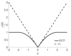
Figure 2: A comparison between the MCP (solid line) and the $\ell_{1}$ penalty (dashed line).

Throughout, let $\rho(\cdot):=\rho_{\theta}(\cdot)$ be the MCP with two parameters $\theta=(\gamma,\lambda)$ [25]:

$$\rho(x;\gamma,\lambda)=\begin{cases}\lambda|x|-\frac{x^{2}}{2\gamma},&\mbox{$|x|<\gamma\lambda$,}\\ \frac{1}{2}\gamma\lambda^{2},&\mbox{$|x|\geq\gamma\lambda$,}\end{cases}$$ (15)

where $\lambda\geq 0$ and $\gamma>1$. Parameter $\lambda$ measures the penalty level, while $\gamma$ controls the concavity of the function. For a fixed value of $\lambda$, the MCP approaches the $\ell_{1}$ penalty as $\gamma\to\infty$, and the $\ell_{0}$ penalty as $\gamma\to 0^{+}$.

Figure 2 compares the MCP with $(\gamma,\lambda)=(2,1)$ and the $\ell_{1}$ penalty. The right derivative of MCP at zero is $\lambda$, which is the same as the derivative of the $\ell_{1}$ penalty. The MCP function flats out when $|x|\geq\gamma\lambda$.

Remark 1.

Aragam and Zhou [21] use an MCP regularized likelihood to estimate Gaussian DAGs as well. However, rather than searching over permutations, which automatically satisfies the acyclicity constraint, they perform a greedy coordinate descent to minimize the regularized loss over DAGs. Thus, at each update in their algorithm the acyclicity constraint must be carefully checked.

3.3 Likelihood for experimental data

It is well-known that DAGs in the same Markov equivalence class are observationally equivalent, and thus we cannot distinguish such DAGs from observational data alone. However, experimental interventions can help distinguish equivalent DAGs and construct causal networks. Following [26], intervention on a node $X_{j}$ in a DAG is to impose a fixed external distribution on this node, denoted by $p(x_{j}\mid\bullet)$, independent of all $X_{-j}$, while keeping the structural equations (2) of the other nodes unchanged.

Suppose that our data $\mathbf{X}\in\mathbb{R}^{n\times p}$ consists of $M$ blocks, where each block $\mathbf{X}^{m}\in\mathbb{R}^{n_{m}\times p}$ and $n=\sum_{m=1}^{M}n_{m}$. Denote by $X^{m}_{\mathcal{I}}\subseteq\{X_{1},\ldots,X_{p}\}$ the set of variables under experimental interventions in block $m$. Then, the data for $X_{j}\in X^{m}_{\mathcal{I}}$ in this block are generated independently from the distribution $p(x_{j}\mid\bullet)$, while for $X_{i}\notin X_{\mathcal{I}}^{m}$ from the conditional distribution $[X_{i}\mid\Pi_{i}^{\mathcal{G}}]$. Note that multiple nodes could be intervened for a block of data, in which case $|X^{m}_{\mathcal{I}}|\geq 2$.

Let $\mathcal{I}_{j}\subseteq\{1,2,\ldots,n\}$ be the set of observations for which $X_{j}$ is under experimental intervention, and let $\mathcal{O}_{j}=\{1,2,\ldots,n\}\setminus{\mathcal{I}_{j}}$ be its complement. By the truncated factorization formula [27, 26, 23], the joint density of experimental data is

$$p(\mathbf{X})=\prod_{j=1}^{p}\prod_{h\in\mathcal{O}_{j}}p(x_{hj}\mid pa_{hj})\prod_{k\in\mathcal{I}_{j}}p(x_{kj}\mid\bullet),$$ (16)

where $x_{hj}$ is the value of the $j^{\text{th}}$ variable in the $h^{\text{th}}$ observation and $pa_{hj}$ is the value for its parents. Let $\mathbf{X}_{\mathcal{O}_{\pi(j)}}$ be the submatrix of $\mathbf{X}$ with rows in $\mathcal{O}_{\pi(j)}$ and

$$\widehat{\Sigma}^{j}:=\frac{1}{|\mathcal{O}_{\pi(j)}|}\mathbf{X}_{\mathcal{O}_{\pi(j)}}^{\top}\mathbf{X}_{\mathcal{O}_{\pi(j)}}$$

be the sample covariance matrix computed from data in these rows. Then the log-likelihood of experimental data can be re-parametrized into the Cholesky loss functions as well:

Lemma 2.

The negative log-likelihood for experimental data (16) can be written as

$$\ell_{\mathcal{O}}(L,P) =\sum_{j=1}^{p}|\mathcal{O}_{\pi(j)}|\mathscr{L}_{\text{chol}}\left(L_{j};P\widehat{\Sigma}^{j}P^{\top}\right),$$ (17)

where $L_{j}=(e_{j}-\beta_{j})/{\omega_{j}}\in\mathbb{R}^{p}$, $L=(L_{j})\in\mathcal{L}_{p}$, and $|L_{j}|:=L_{jj}$ in $\mathscr{L}_{\text{chol}}(\cdot)$ (9).

See Appendix A.2 for the proof. Though experimental data likelihood $\ell_{\mathcal{O}}(L,P)$ in (17) is not identical to the observational $\ell(L,P)$ in (1), searching strategies described in the next section can be applied on both observational and experimental data.

4 Optimization

We now describe how we solve the optimization problem (14). The main steps are outlined in Algorithm 1, where we use simulated annealing to search over the permutation space for an ordering that minimizes the RC score defined in (13). To obtain the RC score for a given permutation, we need to solve a continuous optimization problem (line 2 and 6) for which we propose a proximal gradient algorithm (Algorithm 2).

4.1 Searching over permutations

Algorithm 1 Annealing on regularized Cholesky score (ARCS).

Input: Dataset $\mathbf{X}$, initial permutation matrix $P_{0}$,

a temperature schedule $\{T^{(i)},i=0,\ldots,N\}$,

constant $m$.
      Output: Adjacency matrix $\widehat{B}$.

1:Select tuning parameters $(\gamma,\lambda)$ for $f(L;P)$ according to Algorithm 4 (Section 4.4).

2:$\widehat{P}\leftarrow P_{0},~{}\widehat{L}\leftarrow\operatorname*{arg\,min}_{L\in\mathcal{L}_{p}}f(L;\widehat{P})$ by Algorithm 2, $f(\widehat{P})\leftarrow f(\widehat{L};\widehat{P})$.

3:for $i=0,\ldots,N$ do

4:     $T\leftarrow T^{(i)}$.

5:     Propose $P^{*}$ by flipping a random length-$m$ interval       in the permutation defined by $\widehat{P}$.

6:     $L^{*}\leftarrow\operatorname*{arg\,min}_{L\in\mathcal{L}_{p}}f(L;P^{*})$ using Algorithm 2,      $f(P^{*})\leftarrow f(L^{*};P^{*})$.

7:     $\alpha\leftarrow\min\left\{1,\exp\big{(}{-}\frac{1}{T}[f(P^{*})-f(\widehat{P})]\big{)}\right\}$.

8:     Set $(\widehat{P},\widehat{L},f(\widehat{P}))\leftarrow(P^{*},L^{*},f(P^{*}))$ with prob. $\alpha$.

9:end for

10:Refine adjacency matrix $\widehat{B}$ given $(\widehat{P},\widehat{L})$ by Algorithm 3 (Section 4.3).

The ARCS algorithm is detailed in Algorithm 1. At each iteration, we propose a permutation $P^{*}$ and decide whether to stay at the current permutation or move to the proposed one with probability $\alpha$ given in line 7. The probability is determined by the difference between the proposed and current scores $f(P^{*})-f(\widehat{P})$ normalized by a temperature parameter $T$. For $T\to\infty$, the jumps are completely random and for $T\to 0^{+}$ completely determined by the RC score $f(\cdot)$. The algorithm follows a temperature schedule which is often taken to be a decreasing sequence $T^{(0)}\geq T^{(1)}\geq\ldots\geq T^{(N)}$ allowing the algorithm to explore more early on and zoom in on a solution as time progresses.

The proposed permutation matrix $P^{*}$ is constructed as follows. Let $\widehat{\pi}$ and $\pi^{*}$ be the permutations associated with $\widehat{P}$ and $P^{*}$ as in (5). We propose $\pi^{*}$ by flipping (i.e., reversing the order of) a random interval of length $m$ in the current permutation $\widehat{\pi}$. For example, with $m=3$ we may flip $\widehat{\pi}=(1,2,3,4,\ldots,p)$ to $\pi^{*}=(1,4,3,2,\ldots,p)$ in the proposal. Equivalently, we flip a contiguous block of $m$ rows of $\widehat{P}$ to generate $P^{*}$.

As a byproduct of evaluating the RC score for the proposed permutation $P^{*}$, we also obtain the corresponding lower triangular matrix $L^{*}$, representing the associated DAG. We keep track of these DAGs as well as the permutations throughout the algorithm (line 6).

4.2 Computing RC score

We propose a proximal gradient algorithm to evaluate the RC score $f(P)$ at each permutation matrix $P$ (line 2 and 6, Algorithm 1). This algorithm belongs to a class of first-order methods that are quite effective at optimizing functions composed of a smooth loss and a nonsmooth penalty [28].

The RC score is obtained by minimizing the RC loss $f(L;P)$ over $L$ as shown in (13). Recall that $\mathcal{L}_{p}$ is the set of $p\times p$ lower triangular matrices, and let

$$\rho(u):=\sum_{i>j}\rho(u_{ij}),\quad\text{for}\quad u=(u_{ij})\in\mathcal{L}_{p}.$$ (18)

Note that we are leaving out the diagonal elements of $u$ in defining $\rho(u)$. Then, the RC loss is $f(u;P)=\ell(u,P)+\rho(u),$ where $\ell(u,P)$ (1) is differentiable and $\rho(u)$ is nonsmooth. The idea of the proximal gradient algorithm is to replace $\ell(u,P)$ with a local quadratic function at the current estimate $L$ and optimize the resulting approximation to $f(u;P)$ to get a new estimate $L^{+}$:

$$L^{+} =\operatorname*{arg\,min}_{u\in\mathcal{L}_{p}}\ell(L)+\nabla\ell(L)^{\top}(u-L)+\frac{1}{2t}\lVert u-L\lVert^{2}+\rho(u)$$

$$=\operatorname*{arg\,min}_{u\in\mathcal{L}_{p}}\frac{1}{2t}\left\|L-t\nabla\ell(L)-u\right\|^{2}+\rho(u),$$ (19)

where $\ell(L)=\ell(L,P),\nabla\ell(L):=\nabla_{L}\ell(L,P)$ is the gradient of $\ell(L,P)$ w.r.t. $L$, and $t>0$ is a step size. Consider the proximal operator $\operatorname{\mathbf{prox}}_{\rho}:\mathcal{L}_{p}\to\mathcal{L}_{p}$ associated with $\rho$ defined by

$$\operatorname{\mathbf{prox}}_{\rho}(x):=\operatorname*{arg\,min}_{u\in\mathcal{L}_{p}}\left(\rho(u)+\frac{1}{2}\lVert x-u\lVert^{2}\right),$$

where $x\in\mathcal{L}_{p}$ and $\lVert\ \cdot\ \lVert$ is the usual Euclidean norm. Then, (4.2) is equivalent to

$$L^{+}=\operatorname{\mathbf{prox}}_{t\rho}\left(L-t\nabla\ell(L)\right),$$ (20)

where $\operatorname{\mathbf{prox}}_{t\rho}(\cdot)$ is the proximal operator applied to the scaled function $t\rho(\cdot)$. Since $\rho(u)$ is separable across the coordinates $\{u_{ij},i\geq j\}$, we have for $x\in\mathcal{L}_{p}$,

$$\left(\operatorname{\mathbf{prox}}_{\rho}(x)\right)_{ij}=\begin{cases}\operatorname{\mathbf{prox}}_{\rho}(x_{ij}),&i>j,\\ \operatorname{\mathbf{prox}}_{0}(x_{ii})=x_{ii},&i=j.\end{cases}$$

The proximal operators on the RHS are univariate, and the distinction between the two cases is because we do not penalize the diagonal entries, i.e., $\rho(u_{ii})=0$.

Algorithm 2 Compute the RC score by proximal gradient.

Input: $P$, $L^{(0)}\in\mathcal{L}_{p}$, $t^{(0)}>0$, $\kappa\in(0,1)$, max-iter,                  tol.
      Output: $L$.

1:$k\leftarrow 0$, err $\leftarrow\infty$, $L\leftarrow L^{(0)}.$

2:while $k<$ max-iter and err $>$ tol do

3:     Compute $\nabla\ell(L)$ using either Lemma 3 or 4.

4:     $t\leftarrow t^{(0)}/{\lVert\nabla\ell(L)\lVert_{F}}$.

5:     repeat

6:         $\widetilde{L}\leftarrow L-t\nabla\ell(L)$.

7:         $L^{+}_{ij}\leftarrow\operatorname{\mathbf{prox}}_{t\rho}(\widetilde{L}_{ij})$ for $i>j$ (using Lemma 5).

8:         $L^{+}_{ii}\leftarrow\widetilde{L}_{ii}$.

9:         break if $\ell\left(L^{+},P\right)\leq\ell\left(L,P\right)+\left\langle{\nabla\ell(L)},L^{+}-L\right\rangle$                                                $+\frac{1}{2t}\|L^{+}-L\|^{2}_{F}$.

10:         $t\leftarrow\kappa t$.

11:     err $\leftarrow\max_{j}\delta(L_{j}^{+},L_{j})$ where $\delta(x,y):=\frac{\left\|x-y\right\|}{\max\{1,\left\|y\right\|\}}$.

12:     $L\leftarrow L^{+}$ and $k\leftarrow k+1$.

13:end while

The overall procedure is summarized in Algorithm 2. To choose the step size $t$ normalized by $\lVert\nabla\ell(L)\lVert_{F}$ (line 4), we have used a line search strategy [28], where we repeatedly reduce the step size by a factor $\kappa\in(0,1)$ until a quadratic upper bound is satisfied by the new update (line 9). To implement Algorithm 2, we need two more ingredients, $\nabla\ell(L)$ and the univariate $\operatorname{\mathbf{prox}}_{\rho}(\cdot)$, both of which have nice closed-form expressions:

Lemma 3.

The gradient of $\ell(L,P)$ in (1) w.r.t. $L$ is

$$\nabla\ell(L)=n\left({\Pi_{\mathcal{L}}}(P\widehat{\Sigma}P^{\top}L)-\operatorname{diag}\left(\{1/L_{ii}\}_{i=1}^{p}\right)\right),$$

where $\Pi_{\mathcal{L}}:A\mapsto(A_{ij}\mathbbm{1}\{i\geq j\})_{p\times p}$ maps a matrix to its lower triangular projection.

Lemma 4.

The gradient of $\ell_{\mathcal{O}}(L,P)$ in (17) w.r.t. $L_{j}$ is

$$\nabla_{L_{j}}\ell_{\mathcal{O}}(L,P)=\left|\mathcal{O}_{\pi(j)}\right|\left(\Pi_{j}\big{(}P\widehat{\Sigma}^{j}P^{\top}L_{j}\big{)}-\frac{e_{j}}{L_{jj}}\right),$$

where $\Pi_{j}:v\mapsto(v_{i}\mathbbm{1}\{i\geq j\})_{p\times 1}$ and $\{e_{j}\}$ is the canonical basis of $\mathbb{R}^{p}$.

Lemma 5.

Let $\rho$ be the scalar MCP with parameter $(\gamma,\lambda)$ defined in (15), and let $\rho_{1}$ be the same penalty for $\lambda=\gamma=1$. Then, for any $t>0$,

$$\operatorname{\mathbf{prox}}_{t\rho}(x)=\lambda\gamma\operatorname{\mathbf{prox}}_{(t/\gamma)\rho_{1}}\Big{(}\frac{x}{\lambda\gamma}\Big{)},$$ (21)

and for any $\alpha>0$,

$$\operatorname{\mathbf{prox}}_{\alpha\rho_{1}}(x)=\begin{cases}0,&\parbox[c]{108.405pt}{ $0\leq x<\min\{\alpha,1\}\text{ or }\\ 1<x<\sqrt{\alpha};$}\\ \dfrac{x-\alpha}{1-\alpha},&\alpha<x\leq 1;\\ x,&\parbox[c]{108.405pt}{$x>\max\{\alpha,1\}\text{ or }\\ 1<\sqrt{\alpha}<x\leq\alpha.$}\end{cases}$$ (22)

Moreover, $\operatorname{\mathbf{prox}}_{\alpha\rho_{1}}(-x)=-\operatorname{\mathbf{prox}}_{\alpha\rho_{1}}(x)$ for all $x\in\mathbb{R}$.

We have excluded two special cases in (22) in which the minimizer is not unique: 1) If $x=\alpha=1$, $\operatorname{\mathbf{prox}}_{\alpha\rho_{1}}(x)=[0,1]$; 2) If $x=\sqrt{\alpha}>1$, $\operatorname{\mathbf{prox}}_{\alpha\rho_{1}}(x)=\{0,\sqrt{\alpha}\}$. We set $\operatorname{\mathbf{prox}}_{\alpha\rho_{1}}(x)=0$ in our implementation if these special cases occur. The MCP has parameter $\gamma>1$, and usually the step size $t<1$. Thus, the cases with $\alpha<1$ are the most common scenario in our numerical study. These lemmas are proved in Appendix A.3, A.4, and A.5.

4.3 Structure refinement after annealing

At the end of the annealing loop (line 9, Algorithm 1), a pair $(\widehat{P},\widehat{L})$ is found which minimizes the RC score (14). Accordingly, an estimated reversal of a topological sort is $\widehat{\pi}=\widehat{P}(1,\ldots,p)^{\top}$. Define $\widetilde{L}=\widehat{P}^{\top}\widehat{L}\widehat{P}$, and $\widehat{B}$ by $\widehat{B}_{ij}=-{\widetilde{L}_{ij}}/{\widetilde{L}_{jj}}$ for $i\neq j$ and $\widehat{B}_{ii}=0$. Then, $\widehat{B}$ is the estimated weighted adjacency matrix for a DAG, i.e., an estimate for $B_{0}$. The support of $\widehat{B}$ gives the estimated parent sets $\widehat{pa}_{j}=\{i:\widehat{B}_{ij}\neq 0\}$ for $j=1,\ldots,p$. The use of a continuous regularizer, i.e. MCP, eases our optimization problem; however, this may lead to more false positive edges compared to $\ell_{0}$ regularization. To improve structure learning accuracy, we add a refinement step to remove some predicted edges by conditional independence tests, which borrows the strength from a constraint-based approach.

The refinement step outlined in Algorithm 3 is based on the following fact. If $k\prec j$ in a topological sort and there is no edge $k\to j$, then $X_{k}\perp X_{j}\mid\Pi_{j}$, where $\Pi_{j}$ is the parent set of $X_{j}$. For each $k\in\widehat{pa}_{j}$, we test the null hypothesis that $X_{k}$ and $X_{j}$ are conditionally independent given $\widehat{pa}_{j}\setminus\{k\}$ using the Fisher Z-score. We remove the edge $k\to j$ if the null hypothesis is not rejected at a given significance level. The conditional independence tests are performed in a sequential manner for the nodes in $\widehat{pa}_{j}$ according to the estimated topological sort: For $k_{1},k_{2}\in\widehat{pa}_{j}$, if $k_{1}\prec k_{2}$ in the sort, we carry out the test for $k_{2}$ prior to that for $k_{1}$.

Algorithm 3 Constraint-based structure refinement.

Input: Dataset $\mathbf{X}$, permutation ${\widehat{\pi}}$, adjacency matrix $\widehat{B}$,
                 significance level $\alpha$.
      Output: Adjacency matrix $\widehat{B}$.

1:$Z_{\alpha}\leftarrow\Phi^{-1}(1-\frac{\alpha}{2})$, where $\Phi(x)$ is the CDF of $\mathcal{N}(0,1)$.

2:for $j=1,\ldots,p$ do

3:     $\widehat{pa}_{j}\leftarrow\{i:\widehat{B}_{ij}\neq 0\}$.

4:     for $k\in\widehat{pa}_{j}$ do

5:         $\mathbf{s}\leftarrow\widehat{pa}_{j}\setminus\{k\}$.

6:         $\mathbf{X}^{j}\leftarrow$ observations for which $j$ is not intervened

7:         $n\leftarrow$ number of rows in $\mathbf{X}^{j}$.

8:         $r_{j,k\mid\mathbf{s}}\leftarrow$ sample partial correlation between $X_{j}$           and $X_{k}$ given $X_{\mathbf{s}}$ based on $\mathbf{X}^{j}$.

9:         $z\leftarrow\frac{1}{2}\sqrt{n-|\mathbf{s}|-3}\log\left(\frac{1+r_{j,k\mid\mathbf{s}}}{1-r_{j,k\mid\mathbf{s}}}\right)$.

10:         Remove $k$ from $\widehat{pa}_{j}$, if $|z|<Z_{\alpha}$.      

11:     end for

12:     $\widehat{B}_{ij}\leftarrow 1$ if $i\in\widehat{pa}_{j}$ and $\widehat{B}_{ij}\leftarrow 0$ otherwise.

13:end for

4.4 Selection of the tuning parameters

Before starting the iterations in Algorithm 1, we select and fix the tuning parameters $\theta=(\gamma,\lambda)$ of MCP (line 1), hence fixing a particular scoring function $f(L,P)=f_{\theta}(L,P)$ throughout the algorithm.

Algorithm 4 Tuning parameter selection by BIC.

Input: Initial permutation $P_{0}$ and a grid of values
                 $\{\theta^{(i)}\}=\{(\gamma^{(i)},\lambda^{(i)})\}$.
      Output: Optimal index $i^{*}$ in the grid.

1:Define $\widehat{L}(\theta):=\operatorname*{arg\,min}_{L\in\mathcal{L}_{p}}\,f_{\theta}(L;P_{0})$ computed by Algorithm 2.

2:Let $\text{BIC}(\theta):=2\ell\big{(}\widehat{L}(\theta);P_{0}\big{)}+\|\widehat{L}(\theta)\|_{0}\log\left(\max\{n,p\}\right).$

3:Output $i^{*}=\operatorname*{arg\,min}_{i}\text{BIC}(\theta^{(i)})$.

We use the Bayesian information criterion (BIC) [29] to select the tuning parameters, given an initial permutation $P_{0}$. The details are summarized in Algorithm 4. For every pair $(\gamma^{(i)},\lambda^{(i)})$ over a grid of values, we evaluate the BIC score given in line 2, where $\|\widehat{L}(\cdot)\|_{0}$ is the number of nonzero entries in $\widehat{L}(\cdot)$, and then we output the one with the lowest BIC score. The regularization parameter in BIC($\theta$) is adapted to $\log(\max\{n,p\})$, which works well for both low and high-dimensional data. To construct the grid, possible choices for the concavity parameter $\gamma$ are $\{2,10,50,100\}$ based on our tests. Note that $\gamma>1$ is required in the definition of MCP (15), while the behavior of MCP for $\gamma\geq 100$ is essentially the same as the $\ell_{1}$ penalty. For the regularization parameter $\lambda$, we select 20 equi-spaced points from the interval $[0.1\sqrt{n},\sqrt{n}]$. The choice of $\sqrt{n}$ often leads to an empty graph when the data are standardized, hence a natural end point.

5 Results

5.1 Methods and data

Recall that $p$ is the number of variables and $n$ is the number of observations. For a thorough evaluation of the algorithm, we simulated data for both $n>p$ and $n<p$ cases.

We used real and synthetic networks to simulate data. Real networks were downloaded from the Bayesian networks online repository [30]. We duplicated some of them to further increase the network size. Synthetic DAG structures were constructed using the sparsebn package [31]. Given a DAG structure, we sampled the edge coefficients $\beta_{ij}$ uniformly from $[-0.8,-0.5]\cup[0.5,0.8]$ and set the noise variance to one. We then calculated the covariance matrix according to (4) and normalized its diagonal elements to one. Consequently, the variances of $\{X_{1},\ldots,X_{p}\}$ were identical. We used the following networks to generate observational data, denoted by the network name and $(p,s_{0})$, where $s_{0}$ is the number of edges after duplication: 4 copies of Hailfinder (224, 264), 1 copy of Andes (223, 338), 2 copies of Hepar2 (280, 492), 4 copies of Win95pts (304, 448), 1 copy of Pigs (441, 592), and random DAGs, rDAG1 (300, 300) and rDAG2 (300, 600).

In the observational data setting, we compared our algorithm with the following BN learning algorithms: the coordinate descent (CD) algorithm [21], the standard greedy hill climbing (HC) algorithm [5], the greedy equivalence search (GES) [6], the Peter-Clark (PC) algorithm [1], the max-min hill-climbing (MMHC) algorithm [4], and the genetic algorithm (GA) [15].

The CD algorithm optimizes a regularized log-likelihood function by a blockwise update on $(\beta_{ij},\beta_{ji})$ while checking the acyclicity constraint before each update. The HC algorithm performs a greedy search over the DAG space by starting from a certain initial state, performing a finite number of local changes and selecting the DAG with the best improvement in each local change. The GES algorithm searches over the equivalence classes and utilizes greedy search operators on the current state to find the next one, of which the output is an equivalence class of DAGs. The PC algorithm performs conditional independence tests to identify edges and orients edge directions afterwards. The MMHC algorithm constructs the skeleton of a Bayesian network via conditional independence tests and then performs a greedy hill climbing search to orient the edges via optimizing a Bayesian score. The GA decomposes graph estimation into two optimization sub-problems: node ordering search with mutation and crossover operators, and structure optimization by an adaption of the least angle regression [22].

Among these methods, PC is a constraint-based method, and MMHC is a hybrid method. Other methods, CD, HC, GES and GA, are all score-based, where CD and HC search over the DAG space, GES searches over the equivalence classes, and GA searches over the permutation space. Our method is a score-based search over the permutation space, similar to GA.

Our ARCS algorithm (Algorithm 1) may take an initial permutation $P_{0}$ provided by a local search method. In this study, we use the CD and GES algorithms to provide an initial permutation, and call the corresponding implementation ARCS(CD) and ARCS(GES). To partially preserve properties of the input initial permutation, we start with a low temperature $T^{(0)}=1$. The output of the CD algorithm is a DAG for which we find a topological sort to define $P_{0}$. The GES algorithm outputs a completed partially directed acyclic graph (CPDAG). We then generate a DAG in the equivalence class of the estimated CPDAG, and initialize ARCS with a topological sort of this DAG.

We implemented the ARCS algorithm in Matlab, and used the following R packages for other methods: sparsebn [31] for the CD algorithm, rcausal [32] for the GES, GIES (for experimental data) and PC algorithms, bnlearn [33] for the MMHC and HC algorithms, and GADAG [15] for the GA.

5.2 Accuracy metrics

Among all methods applied on observational data, ARCS, CD, HC and MMHC output DAGs, while the GES and PC algorithms output CPDAGs. Given these estimates, we need to evaluate the performance of each method. Define P, TP, FP, M, R as the numbers of estimated edges, true positive edges, false positive edges, missing edges and reverse edges, respectively. To standardize the performance metrics in observational data setting, we consider both directed and undirected edges in the definitions of these metrics as follows.

P is the number of edges in the estimated graph. FP is the number of edges in the estimated graph skeleton but not in the true skeleton. M counts the number of edges in the true skeleton but not in the skeleton of the estimated graph. We define an estimated directed edge to be true positive (TP) if it meets either of the two criteria: 1) This edge is in the true DAG with the same orientation; 2) This edge coincides after converting the estimated graph and true DAG to CPDAGs. An estimated undirected edge is considered TP if it satisfies the second condition. Note that our criterion takes into account reversible edges in an equivalence class for observational data. Lastly, the number of reversed edges $\text{R}=\text{P}-\text{TP}-\text{FP}$.

Denote by $s_{0}$ the number of edges in the true DAG. The overall accuracy of a method is measured by the structural Hamming distance (SHD) and Jaccard index (JI), where $\text{SHD}=\text{R}+\text{FP}+\text{M}$ and $\text{JI}=\text{TP}/(s_{0}+\text{P}-\text{TP})$. A method has better performance if it achieves a lower SHD and/or a higher JI.

5.3 Comparison on observational data

We used large networks, where $p\in(200,450)$ and $s_{0}\in(250,600]$, to simulate observational data with $n<p$ and $n>p$. For each setting $(p,s_{0},n)$, we generated 20 datasets, and ran CD, ARCS(CD), GES, ARCS(GES) and other methods (PC, HC, MMHC and GA) with a maximum time allowance of 10 minutes per dataset. The HC and MMHC algorithms had an upper-bound of the in-degree number as 2. We tried a higher maximum in-degree, but it resulted in a large FP. MMHC and PC were run with a significance level of 0.01 in conditional independence tests. We ran the CD algorithm with an MCP regularized likelihood, in which $\gamma=2$ and $\lambda$ was chosen by a default model selection mechanism. GA was run for a maximum of $10^{4}$ iterations, using the default population size and the default rates of mutation and crossover. We tried a larger population size for GA, but it was too time-consuming.

Our methods, ARCS(CD) and ARCS(GES), initialized with permutations from CD and GES estimates, were run for a maximum of $10^{4}$ iterations, with initial temperature $T^{(0)}=1$ and reversal length $m=4$ (Algorithm 1). A $p$-value cutoff of $10^{-5}$ was used in the refinement step (Algorithm 3). For the networks we considered, on average, 500 tests were performed in the refinement step, and the cutoff was chosen by Bonferroni correction to control the familywise error rate at level 0.005. In fact, our results were almost identical for any $p$-value cutoff between $10^{-3}$ and $10^{-5}$.

TABLE I: Comparison between ARCS and initial estimates on observational data ($n<p$).

network	method	P	TP	R	FP	SHD	JI
$(p,s_{0},n)$
Hailfinder	CD	270	154	84	32	142	0.41
$(224,264,200)$	ARCS(CD)	274	187	54	33	110	0.53
	GES	243	184	49	10	89	0.57
	ARCS(GES)	261	215	30	16	65	0.70
Andes	CD	352	176	108	68	230	0.34
$(223,338,200)$	ARCS(CD)	368	233	71	65	170	0.50
	GES	272	220	35	17	135	0.57
	ARCS(GES)	334	276	31	27	89	0.70
Hepar2	CD	495	245	120	130	377	0.33
(280,492,200)	ARCS(CD)	500	311	107	82	264	0.46
	GES	410	253	96	62	302	0.39
	ARCS(GES)	483	324	96	64	232	0.50
Win95pts	CD	399	195	154	50	302	0.30
$(304,448,200)$	ARCS(CD)	465	317	88	59	190	0.53
	GES	335	244	71	21	225	0.45
	ARCS(GES)	451	361	57	34	121	0.67
Pigs	CD	715	342	207	166	417	0.36
$(441,592,200)$	ARCS(CD)	587	421	123	43	214	0.55
	GES	581	431	112	38	199	0.58
	ARCS(GES)	575	454	94	27	165	0.63
rDAG1	CD	319	208	85	25	117	0.51
$(300,300,240)$	ARCS(CD)	305	260	36	9	49	0.76
	GES	283	268	14	1	33	0.85
	ARCS(GES)	297	283	13	1	18	0.90
rDAG2	CD	715	407	136	171	364	0.50
$(300,600,240)$	ARCS(CD)	623	498	73	52	154	0.69
	GES	505	474	26	6	132	0.75
	ARCS(GES)	594	564	18	13	49	0.89

• In this and all subsequent tables, reported results are rounded averages over 20 datasets; the best SHD and JI for each network are highlighted in boldface.

ARCS versus CD and GES. Table I reports the average performance metrics across 20 datasets for 7 networks (5 real and 2 random networks) in the high-dimensional setting $n<p$ using CD, ARCS(CD), GES and ARCS(GES). We were interested in the potential improvement of ARCS upon its initial permutations. It is indeed confirmed by the results in the table that ARCS(CD) and ARCS(GES) outperformed CD and GES, respectively, for every network, achieving lower SHDs and higher JIs. The reduction in SHD was very substantial, close to or above 40%, for many networks, such as Win95pts, Pigs, rDAG1 and rDAG2.

The same comparison was done for low-dimensional settings with $n>p$, reported in Table II. We observe similar improvements of ARCS(CD) and ARCS(GES) over CD and GES, consistent with the results for high-dimensional data. It is seen from both tables that ARCS always increased TP, while maintaining or slightly reducing FP. The annealing process often identified more TP edges, while the refinement step (Algorithm 3) cut down the FP edges given the ordering and parent sets learned through simulated annealing.

TABLE II: Comparison between ARCS and initial estimates on observational data ($n>p$).

network	method	P	TP	R	FP	SHD	JI
$(p,s_{0},n)$
Hailfinder	CD	278	156	88	34	142	0.41
$(224,264,400)$	ARCS(CD)	296	196	59	41	109	0.54
	GES	272	201	53	18	81	0.60
	ARCS(GES)	273	232	26	15	47	0.76
Andes	CD	366	189	107	70	220	0.37
$(223,338,400)$	ARCS(CD)	376	242	69	66	162	0.53
	GES	342	273	33	36	102	0.67
	ARCS(GES)	348	296	26	26	69	0.76
Hepar2	CD	519	267	130	122	347	0.36
(280,492,400)	ARCS(CD)	523	330	106	87	248	0.49
	GES	509	312	113	84	264	0.45
	ARCS(GES)	505	336	95	75	231	0.51
Win95pts	CD	398	205	154	39	282	0.32
$(304,448,500)$	ARCS(CD)	542	334	97	111	225	0.51
	GES	472	332	76	64	180	0.56
	ARCS(GES)	475	390	47	38	96	0.73
Pigs	CD	755	353	224	179	418	0.36
$(441,592,600)$	ARCS(CD)	631	451	123	57	198	0.59
	GES	645	467	122	57	182	0.61
	ARCS(GES)	619	471	102	46	166	0.64
rDAG1	CD	319	211	84	24	113	0.52
$(300,300,450)$	ARCS(CD)	319	264	36	20	56	0.74
	GES	299	283	14	2	19	0.90
	ARCS(GES)	300	287	12	1	14	0.92
rDAG2	CD	605	403	140	62	258	0.50
$(300,600,600)$	ARCS(CD)	696	510	79	106	196	0.65
	GES	596	559	20	17	57	0.88
	ARCS(GES)	608	583	14	11	28	0.93

Figure 3 shows the clear improvement of the ARCS algorithm over CD and GES for the Andes and Win95pts networks with more choices of the sample size $n$. Each boxplot summarizes the SHDs over 20 datasets (excluding outliers). For all $n$, ARCS(GES) had a lower SHD than GES, and ARCS(CD) had a lower SHD than CD. The SHD distributions were well-separated, supporting the conclusion that ARCS significantly improves the accuracy of its initial estimates.

Figure 3: Boxplots of SHDs for CD, ARCS(CD), GES and ARCS(GES) on observational data from two networks.

TABLE III: ARCS against others on observational data ($n<p$).

network	method	P	TP	R	FP	SHD	JI
$(p,s_{0},n)$
Hailfinder	ARCS(GES)	261	215	30	16	65	0.70
$(224,264,200)$	HC	414	120	116	179	324	0.21
	PC	227	127	83	17	154	0.35
	GA	193	68	54	71	266	0.18
Andes	ARCS(GES)	334	276	31	27	89	0.70
$(223,338,200)$	HC	422	140	125	158	356	0.23
	MMHC	257	146	98	13	205	0.33
	PC	276	120	137	18	236	0.24
	GA	214	77	67	70	331	0.16
Hepar2	ARCS(GES)	483	324	96	64	232	0.50
$(280,492,200)$	HC	540	153	175	212	551	0.17
	PC	310	108	149	53	436	0.16
	MMHC	269	108	135	26	410	0.17
	GA	434	103	85	246	636	0.10
Win95pts	ARCS(GES)	451	361	57	34	121	0.67
$(304,448,200)$	HC	581	140	206	235	544	0.16
	MMHC	342	146	172	25	327	0.23
	PC	369	114	221	35	369	0.16
	GA	255	108	87	60	400	0.18
Pigs	ARCS(GES)	575	454	94	27	165	0.63
$(441,592,200)$	HC	856	367	168	322	546	0.34
	GA	437	135	127	175	632	0.15
rDAG1	ARCS(GES)	297	283	13	1	18	0.90
$(300,300,240)$	HC	562	135	155	273	438	0.19
	MMHC	316	143	144	28	188	0.30
	PC	328	166	126	36	170	0.36
	GA	175	89	56	30	242	0.23
rDAG2	ARCS(GES)	594	564	18	13	49	0.89
$(300,600,240)$	HC	577	277	170	131	454	0.31
	MMHC	455	307	143	5	298	0.41
	PC	512	162	341	9	446	0.17
	GA	313	141	106	67	526	0.18

• If a method is absent for a network, that means, it took more than 10 minutes to run on a singe dataset, and thus is excluded from the comparison.

ARCS(GES) versus HC, PC, MMHC and GA. We also compared ARCS(GES) with other existing methods, including HC, PC, MMHC and GA. Table III summarizes the average performance on high-dimensional observational data. Among all the methods, ARCS(GES) achieved the lowest SHD and the highest JI for all networks. The HC algorithm tended to output a denser DAG than the truth, leading to a large FP. The PC algorithm had a relatively large number of reverse edges, causing a high SHD. The MMHC algorithm had a lower SHD than some other algorithms, but the SHD difference between ARCS(GES) and MMHC was still large. The PC and MMHC algorithms were slow for some networks, and thus are absent in the results for these networks. The GA was formulated in a similar way as ARCS(GES), but the TPs of GA estimates were much lower, resulting in large SHDs for the tested networks.

Table IV summarizes the results for the low-dimensional setup, $n>p$. It confirms that ARCS(GES) outperforms competing algorithms by a great margin. In general, HC had a larger P and GA had a smaller P than the true DAG, which indicates that their estimates were either too dense or too sparse. That the GA estimates were too sparse is more pronounced in this setting compared to the high-dimensional case. This might be related to its tuning parameter choice.

TABLE IV: ARCS against others on observational data ($n>p$).

network	method	P	TP	R	FP	SHD	JI
$(p,s_{0},n)$
Hailfinder	ARCS(GES)	273	232	26	15	47	0.76
$(224,264,400)$	HC	409	118	121	170	317	0.21
	PC	256	167	70	18	115	0.48
	GA	138	63	47	27	228	0.19
Andes	ARCS(GES)	348	296	26	26	69	0.76
$(223,338,400)$	HC	419	145	125	148	341	0.24
	MMHC	286	169	104	14	184	0.37
	PC	308	154	135	19	203	0.31
	GA	153	64	56	33	307	0.15
Hepar2	ARCS(GES)	505	336	95	75	231	0.51
(280,492,400)	HC	535	152	180	203	544	0.17
	PC	354	125	180	49	416	0.17
	MMHC	317	137	152	28	384	0.20
	GA	416	114	84	218	597	0.10
Win95pts	ARCS(GES)	475	390	47	38	96	0.73
$(304,448,500)$	HC	576	140	223	213	522	0.16
	MMHC	394	164	208	23	307	0.24
	PC	433	153	247	33	328	0.21
	GA	138	71	56	11	389	0.14
Pigs	ARCS(GES)	619	471	102	46	166	0.64
$(441,592,600)$	HC	843	377	164	302	517	0.36
	GA	218	112	83	23	503	0.16
rDAG1	ARCS(GES)	300	287	12	1	14	0.92
$(300,300,450)$	HC	549	186	105	257	371	0.28
	MMHC	324	209	85	29	120	0.51
	PC	335	210	88	37	127	0.50
	GA	135	81	47	7	226	0.20
rDAG2	ARCS(GES)	608	583	14	11	28	0.93
$(300,600,600)$	HC	577	274	177	126	452	0.30
	MMHC	483	314	165	5	291	0.41
	PC	574	268	298	7	339	0.30
	GA	144	88	51	5	516	0.13

It is worth mentioning that ARCS(GES) outperformed other methods substantially for larger networks such as Pigs with $p=441$ and $s_{0}=592$. MMHC and PC failed to complete a single run on the Pigs network within 10 minutes, while HC and GA had very low accuracies. We suspect that the Pigs network has a certain structure that is particularly difficult to estimate, a hypothesis that merits more investigation.

We also tested another order-based algorithm, linear structural equation model learning (LISTEN) [34], which estimates Gaussian DAG structure by a sequential detection of ordering. A key assumption of LISTEN is that the noise variables have equal variances. Moreover, the algorithm requires a prespecified regularization parameter for the score metric. To compare with this algorithm, we adapted our data generation process to satisfy the equal-variance assumption. ARCS(GES) achieved a much higher accuracy, with SHD as small as 14% to 18% of the SHD achieved by LISTEN. Full results are reported in the supplementary material.

5.4 Comparison on experimental data

To generate experimental datasets, we generated $p$ blocks of observations, in each of which a single variable was under intervention. For each block, we generated 5 observations, and thus $n=5p$. Networks in this experiment were smaller, with $p\leq 50$ and $s_{0}\leq 100$, including real DAGs $(p,s_{0})$: Asia (8, 8), Sachs (11, 17), Ins.(27, 52), Alarm (37, 46), and Barley (48, 84), and random DAGs: rDAG3 (20, 20), rDAG4 (20, 40), rDAG5 (50, 50) and rDAG6 (50, 100). Using these networks, we also simulated observational data of the same sample size, $n=5p$, to study the effect of experimental interventions. Since networks in the experimental setting were smaller, we used a $p$-value cutoff of $10^{-3}$ in the refinement step of the ARCS algorithm (Algorithm 3).

To assess the accuracy on experimental data, we compare an estimated DAG with the true one to calculate the numbers of false positives (FP), missing edges (M), reverse edges (R) and true positives (TP). FP and M follow the same calculations as in the observational settings. R counts the number of edges whose orientations are opposite between the two DAGs, and $\text{TP}=\text{P}-\text{R}-\text{FP}$. Note that the definition of R is different from that for observational data, because under the intervention setting used in this comparison, the true causal DAG is identifiable [20]. The structural Hamming distance (SHD) and the Jaccard index (JI) are then calculated as in the observational case.

In this setting, we compared ARCS with the CD algorithm [20] and the greedy interventional equivalence search (GIES) algorithm [35], both of which can handle experimental interventions. We initialize ARCS with CD and GIES estimates and call them ARCS(CD) and ARCS(GIES), respectively.

TABLE V: Performance comparison on experimental data.

network	method	P	TP	R	FP	SHD	JI
$(p,s_{0},n)$
Asia	CD	14	6	1	7	8	0.47
$(8,8,40)$	ARCS(CD)	5	5	1	0	4	0.53
	GIES	9	1	6	2	9	0.07
	ARCS(GIES)	5	5	1	0	4	0.53
Sachs	CD	23	9	5	10	17	0.34
$(11,17,55)$	ARCS(CD)	12	10	2	1	8	0.50
	GIES	17	4	10	4	17	0.13
	ARCS(GIES)	12	10	2	1	8	0.51
Ins.	CD	56	30	12	14	36	0.39
$(27,52,135)$	ARCS(CD)	54	40	7	7	18	0.63
	GIES	72	14	34	24	62	0.13
	ARCS(GIES)	57	38	10	10	24	0.56
Alarm	CD	51	35	9	7	16	0.57
$(37,46,185)$	ARCS(CD)	48	43	3	2	5	0.86
	GIES	70	6	40	24	65	0.05
	ARCS(GIES)	51	40	6	6	12	0.70
Barley	CD	85	52	17	16	48	0.45
$(48,84,240)$	ARCS(CD)	103	67	13	23	41	0.58
	GIES	146	21	58	67	129	0.10
	ARCS(GIES)	122	44	35	44	84	0.28
rDAG3	CD	25	15	5	6	11	0.49
$(20,20,100)$	ARCS(CD)	20	18	1	1	2	0.84
	GIES	29	4	15	10	25	0.09
	ARCS(GIES)	20	18	2	1	3	0.83
rDAG4	CD	43	25	8	10	24	0.45
$(20,40,100)$	ARCS(CD)	39	34	3	2	8	0.76
	GIES	48	6	30	11	46	0.07
	ARCS(GIES)	38	35	2	1	6	0.82
rDAG5	CD	55	39	10	6	17	0.60
$(50,50,250)$	ARCS(CD)	51	48	2	1	3	0.90
	GIES	87	7	43	37	80	0.05
	ARCS(GIES)	52	47	3	2	5	0.86
rDAG6	CD	101	70	17	13	43	0.54
$(50,100,250)$	ARCS(CD)	106	94	5	7	12	0.86
	GIES	155	15	81	58	143	0.06
	ARCS(GIES)	159	59	36	64	105	0.34

Table V compares the CD, ARCS(CD), GIES and ARCS(GIES) algorithms, averaging over 20 datasets for each type of networks. It is seen that both ARCS(GIES) and ARCS(CD) achieved dramatic improvements upon GIES and CD algorithms for every single network. This observation is consistent with the findings from the observational data and further confirms that the ARCS algorithm is a powerful tool for improving local estimates. Different from the observational data results (Table I and II), ARCS(CD) usually had better performance than ARCS(GIES) on experimental data.

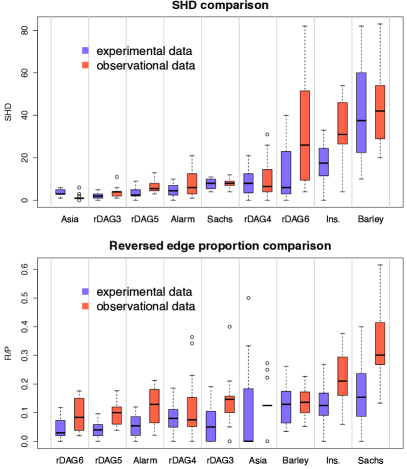
Figure 4: Comparison of SHD and reversed edge proportion between experimental and observational data with ARCS(CD).

Experimental versus observational. We also compared the performance of our method ARCS(CD) on experimental and observational data with the same sample size $n=5p$. Figure 4 plots the SHDs of ARCS(CD) on 20 datasets, with a side-by-side comparison between observational and experimental data. For some networks, such as rDAG6 and Ins., the estimated DAGs using experimental data had much lower SHDs than using the observational data. For some small networks, such as Asia, ARCS(CD) achieved a low SHD on observational data and the improvement when using experimental data was not substantial.

Because estimated DAGs did not have the same number of predicted edges, we further compared the reversed edge proportion ($\text{R}/\text{P}$). The DAGs estimated by ARCS(CD) had a lower R/P on the experimental than the observational data for all networks. The decrease in R/P with experimental interventions was remarkable, as Figure 4 shows. This finding supports the idea that experimental interventions help correct the reversed edges and distinguish equivalent DAGs. Note that for the 20 observational datasets generated from Asia ($p=8$, $s_{0}=8$), ARCS(CD) output 16 estimated DAGs with $\text{P}=8$ and $\text{R}=1$, resulting in a very thin interquantile range in the boxplots of Asia in Figure 4.

5.5 Effectiveness of BIC selection

Given an initial permutation, we use the BIC to choose tuning parameters $(\gamma,\lambda)$ before applying the ARCS algorithm (Section 4.4). In Tables III and IV, the number of predicted edges by ARCS(GES) is closer to $s_{0}$ than any other competing method in every network. This observation signifies the effectiveness of our parameter selection method by BIC. To further study its effect, we compared DAGs estimated with all values on a grid of $(\gamma,\lambda)$ by ARCS(CD) and ARCS(GES).

Figure 5 shows the histograms of the SHDs for all values of $(\gamma,\lambda)$ on Andes datasets with $(p,s_{0})=(223,338)$ and $n\in\{200,400\}$. The grey area in a histogram corresponds to values of $(\gamma,\lambda)$ that led to a lower SHD than the $(\gamma^{*},\lambda^{*})$ chosen by the BIC, i.e., it indicates the percentile of the SHD of the BIC selection among all choices of the tuning parameters. The smaller this percentile, the better the BIC selection performance.

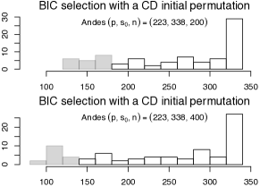
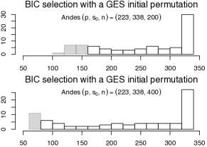
Figure 5: Performance of the BIC selection among a grid of $(\gamma,\lambda)$ given an initial permutation. Tuning parameters that lead to lower SHDs than the BIC selection are shown in gray.

Each histogram has a high spike of large SHD, corresponding to large values of $\lambda$ that generate almost empty graphs. The SHDs of ARCS(CD) with BIC selection corresponded to the $14^{\text{th}}$ and $16^{\text{th}}$ percentiles in low and high dimensions, respectively, and for ARCS(GES) the $16^{\text{th}}$ and $3^{\text{nd}}$ percentiles. These low percentiles confirm that the BIC selection works well for choosing the tuning parameters. Moreover, in our tests, the BIC usually selected $\gamma^{*}=2$, the smallest provided value for $\gamma$. Since for small $\gamma$, the MCP is closer to the $\ell_{0}$ penalty and far from the $\ell_{1}$ norm, this choice of $\gamma$ indicates the preference of concave penalties over $\ell_{1}$ in estimating sparse DAGs. Some of CD’s and GA’s inferior performances, such as CD on the Pigs network (Table I) and the overall performance of GA (Tables III and IV), were potentially caused by a bad choice of their tuning parameters. This demonstrates the importance of our data-driven selection scheme for a regularized likelihood method.

5.6 Random initialization with a high temperature

Recall that we started ARCS(CD) and ARCS(GIES) with $T^{(0)}=1$. To test its global search ability over the permutation space, we may initialize the annealing process with a random permutation and a high temperature, which we denote by ARCS(RND). For a random initial permutation, we do not need to preserve its properties, so we use a high initial temperature $T^{(0)}=100$ to help the algorithm traverse the search space.

We compared ARCS(RND) and ARCS(CD) on experimental data for nine networks. We chose ARCS(CD) due to its superior performance on these networks in the experimental setting (Table V). As shown in Figure 6, ARCS(RND) and ARCS(CD) had comparable performances on all networks. Both of them learned DAGs with small SHDs. ARCS(RND) was slightly better on rDAG4 and Ins., and slightly worse on Alarm and rDAG6. For the other networks, the two methods were quite comparable, demonstrating the effectiveness of ARCS(RND).

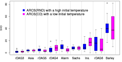
Figure 6: A comparison between ARCS(RND) with a high initial temperature and ARCS(CD) on experimental data.

The networks in this experiment had $p\leq 50$. For $p=50$, there are $50!\approx 3\times 10^{64}$ possible permutations. ARCS(RND) managed to learn a network structure within $10^{4}$ iterations, which is much smaller than $p!$. However, the performance of ARCS(RND) was not competitive on large networks. The reason is that for large $p$, it takes much more time for the annealing to thoroughly search the huge permutation space. Therefore, for large networks, it is better to initialize the ARCS algorithm with estimates from other local methods and choose a low temperature. Given a good initial estimate, ARCS searches over the permutation space and improves the accuracy of the initial estimate as demonstrated in Tables I, II and V. This study suggests that, by combining effective local and global searches under a regularized likelihood framework, our ARCS algorithm is a promising approach to the challenging problem of DAG structure learning.

6 Discussion

In this paper, we developed a method to learn Gaussian BN structures by minimizing the MCP regularized Cholesky score over topological sorts, through a joint iterative update on a permutation matrix and a lower triangular matrix. We search over the permutation space and optimize the network structure encoded by a lower triangular matrix given a topological sort. This approach relates BN learning problem to sparse Cholesky factorization, and provides an alternative formulation for the order-based search. Our method can serve as an improvement of a local search or a stand-alone method with a best-guess initial permutation. Although we formulated this order-based search for Gaussian BNs, it can potentially be extended to discrete BNs and other scoring functions. A main difference in the extension to discrete data is the proximal gradient step, where we can borrow the regularized multi-logit model in [36] or develop a continuous regularizer for multinomial likelihood.

For the simulated annealing step, there are several interesting aspects to investigate. For instance, various operators of moving from one permutation to another have been proposed for greedy order-based search, which could better guide the annealing process in traversing the search space. This paper focuses on numerical results, and shows the advantage and potential application of local search and global annealing in learning BNs. Left as future work are theoretical properties of our method, such as the consistency of the regularized Cholesky score and the convergence of ARCS with a good initial permutation.

Appendix A

A.1 Proof of Proposition 1

Since $A$ is positive definite, $A^{-1}$ is positive definite as well. Let us apply the Cholesky decomposition on $A^{-1}$, i.e., $A^{-1}=CC^{\top}$ where $C=\mathcal{C}(A^{-1})$. Therefore, $A=C^{-\top}C^{-1}$. Recall that $\mathcal{L}_{p}$ is the set of lower triangular matrices with positive diagonals. The goal is to show that the minimizer of $\mathscr{L}_{\text{chol}}(L;A)$ over $\mathcal{L}_{p}$, denoted by $L^{*}$, equals to $C$.

Letting $R=C^{-1}L$, we have $\log|R|=-\log|C|+\log|L|$, where $\log|C|$ is a constant. Since $C\in\mathcal{L}_{p}$ and $L\in\mathcal{L}_{p}$, we have $R\in\mathcal{L}_{p}$ as well. Also,

$$\operatorname{tr}(ALL^{\top}) =\operatorname{tr}(C^{-\top}C^{-1}\ LL^{\top})=\operatorname{tr}(RR^{T})=\left\|R\right\|_{F}^{2}.$$

Then,

$$\min_{L\in\mathcal{L}_{p}}\mathscr{L}_{\text{chol}}(L;A)=\min_{L\in\mathcal{L}_{p}}\left[\frac{1}{2}\operatorname{tr}(ALL^{\top})-\log|L|\right]$$

$$=\min_{R\in\mathcal{L}_{p}}\frac{1}{2}\Big{[}\left\|R\right\|_{F}^{2}-2\log|R|\Big{]}-\log|C|$$

$$=\min_{R\in\mathcal{L}_{p}}\frac{1}{2}\Big{[}\sum_{(i,j):i>j}R_{ij}^{2}+\sum_{i=1}^{p}\left(R_{ii}^{2}-2\log R_{ii}\right)\Big{]}-\log|C|.$$

The problem is separable over entries. Minimizing over off-diagonal entries, the unique minimizer is $R_{ij}^{*}=0$ for all $i>j$ (and clearly $i<j$). Optimizing over $R_{ii}$, we are minimizing $x\mapsto x^{2}-2\log x$ over $x>0$. The unique minimizer is attained at $x=1$, i.e. $R_{ii}^{*}=1$ for all $i$. Therefore the unique minimizer is $R^{*}=I_{p}$, i.e. $C^{-1}L^{*}=I_{p}$. In terms of the original variable, the minimizer is $L^{*}=C=\mathcal{C}(A^{-1})$.

Substituting $L^{*}=\mathcal{C}(A^{-1})$ into $\mathscr{L}_{\text{chol}}(L;A)$, we obtain the minimum value:

$$\mathscr{L}_{\text{chol}}^{*}(A) :=\mathscr{L}_{\text{chol}}(L^{*};A)=\frac{1}{2}\operatorname{tr}\left(AA^{-1}\right)-\log|A^{-\frac{1}{2}}|$$

$$=\frac{1}{2}\left(p+\log|A|\right).$$

The assertion $\mathscr{L}_{\text{chol}}^{*}(A)=\mathscr{L}_{\text{chol}}^{*}(PAP^{\top})$ follows by noting that $|P\widehat{\Sigma}P^{T}|=|P||\widehat{\Sigma}||P^{\top}|=|\widehat{\Sigma}|$.

A.2 Proof of Lemma 2

Recall $B=(\beta_{j})\in\mathbb{R}^{p\times p}$, $\Omega=\operatorname{diag}(\omega_{j}^{2})\in\mathbb{R}^{p\times p}$, we have the following experimental data log-likelihood:

$${~{}}\ell_{\mathcal{O}}(B,\Omega,P_{\pi}\mid\mathbf{X})$$

$$= {~{}}\sum_{j=1}^{p}\frac{1}{2\omega_{j}^{2}}\left\|\mathbf{X}_{\mathcal{O}_{\pi(j)},\pi(j)}-\mathbf{X}_{\mathcal{O}_{\pi(j)}}P_{\pi}^{\top}\beta_{j}\right\|^{2}+\frac{1}{2}|\mathcal{O}_{\pi(j)}|\log\omega_{j}^{2}$$

$$= {~{}}\frac{1}{2}\sum_{j=1}^{p}\bigg{[}\frac{1}{\omega_{j}^{2}}\left\|\mathbf{X}_{\mathcal{O}_{\pi(j)}}P_{\pi}^{\top}(e_{j}-\beta_{j})\right\|^{2}+|\mathcal{O}_{\pi(j)}|\log\omega_{j}^{2}\bigg{]}$$

$$= {~{}}\frac{1}{2}\sum_{j=1}^{p}\bigg{[}\frac{1}{\omega_{j}^{2}}\operatorname{tr}\left(P_{\pi}\mathbf{X}_{\mathcal{O}_{\pi(j)}}^{\top}\mathbf{X}_{\mathcal{O}_{\pi(j)}}P_{\pi}^{\top}(e_{j}-\beta_{j})(e_{j}-\beta_{j})^{\top}\right)$$

$${~{}~{}~{}~{}~{}~{}~{}~{}~{}~{}~{}~{}~{}~{}~{}~{}}+|\mathcal{O}_{\pi(j)}|\log\omega_{j}^{2}\bigg{]}.$$

Recall $L_{j}=(e_{j}-\beta_{j})/\omega_{j}\in\mathbb{R}^{p}$ and $L=(L_{j})\in\mathbb{R}^{p\times p}$. Define $|L_{j}|:=L_{jj}$. Recall $\widehat{\Sigma}^{j}:=\frac{1}{|\mathcal{O}_{\pi(j)}|}\mathbf{X}_{\mathcal{O}_{\pi(j)}}^{\top}\mathbf{X}_{\mathcal{O}_{\pi(j)}}$ and simplify $P_{\pi}$ as $P$. We have

$$\ell_{\mathcal{O}}(L,P) =\frac{1}{2}\sum_{j=1}^{p}|\mathcal{O}_{\pi(j)}|\cdot\left[\operatorname{tr}\big{(}P\widehat{\Sigma}^{j}P^{\top}L_{j}L_{j}^{\top}\big{)}-\log L_{jj}^{2}\right]$$

$$=\sum_{j=1}^{p}|\mathcal{O}_{\pi(j)}|\left[\frac{1}{2}\operatorname{tr}\left(P\widehat{\Sigma}^{j}P^{\top}L_{j}L_{j}^{\top}\right)-\log|L_{j}|\right]$$

$$=\sum_{j=1}^{p}|\mathcal{O}_{\pi(j)}|\mathscr{L}_{\text{chol}}\left(L_{j};P\widehat{\Sigma}^{j}P^{\top}\right),$$

where $\mathscr{L}_{\text{chol}}(L;A)$ is the Cholesky loss defined in (9).

A.3 Proof of Lemma 3

Fix $P$ and let $Z=\frac{1}{\sqrt{n}}\mathbf{X}P^{\top}$ so that $Z^{\top}Z=\frac{1}{n}P\mathbf{X}^{\top}\mathbf{X}P^{\top}=P\widehat{\Sigma}P^{\top}$. We can rewrite (1) as

$$\ell(L):=\ell(L,P)=\frac{n}{2}\left\|ZL\right\|_{F}^{2}-n\log|L|.$$

Let $\ell^{1}(L):=\frac{n}{2}\left\|ZL\right\|_{F}^{2}$ and $\ell^{2}(L):=-n\log|L|$. To compute the gradient of $\ell^{1}$ w.r.t. $L$, we perturb $L$ to $L+t\delta$ where $\delta\in\mathcal{L}_{p}$ and $t\in\mathbb{R}$. We have

$$\lim_{t\to 0}\frac{\ell^{1}(L+t\delta)-\ell^{1}(L)}{t} =\lim_{t\to 0}\Big{[}{n}\left\langle ZL,Z\delta\right\rangle+\frac{tn}{2}\left\|Z\delta\right\|_{F}^{2}\Big{]}$$

$$=n\big{\langle}ZL,Z\delta\big{\rangle}=n\big{\langle}Z^{\top}ZL,\delta\big{\rangle},$$

where $\langle A,B\rangle=\operatorname{tr}(A^{\top}B)$ for two matrices $A$ and $B$. Be definition, $\Pi_{\mathcal{L}}$ maps a $p\times p$ matrix to its lower triangular projection. Since $\delta\in\mathcal{L}_{p}$, $\langle Z^{\top}ZL,\delta\rangle=\langle\Pi_{\mathcal{L}}(Z^{\top}ZL),\delta\rangle$, and thus $\nabla\ell^{1}(L)=n\Pi_{\mathcal{L}}(Z^{\top}ZL)$.

For the second term, $\ell^{2}=-n\sum_{i=1}^{p}\log L_{ii}$, and thus $\nabla\ell^{2}(L)=-n\operatorname{diag}\left(\{1/L_{ii}\}_{i=1}^{p}\right)$ where $L\in\mathcal{L}_{p}$. Putting the pieces together gives the desired result.

A.4 Proof of Lemma 4

From (17), we have $\ell_{\mathcal{O}}=\ell_{\mathcal{O}}^{1}+\ell_{\mathcal{O}}^{2}$, where

$$\ell_{\mathcal{O}}^{1} :=\frac{1}{2}\sum_{j=1}^{p}|\mathcal{O}_{\pi(j)}|L_{j}^{\top}P\widehat{\Sigma}^{j}P^{\top}L_{j},$$

$$\ell_{\mathcal{O}}^{2} :=-\sum_{j=1}^{p}|\mathcal{O}_{\pi(j)}|\log L_{jj}.$$

Note that each term in $\ell_{\mathcal{O}}^{1}$ is a quadratic form in $L_{j}$. The gradient of $\ell^{1}_{\mathcal{O}}$ w.r.t. to $L_{j}$ is $|\mathcal{O}_{\pi(j)}|\Pi_{j}(P\widehat{\Sigma}^{j}P^{\top}L_{j})$, since $L_{ij}=0$ for $i<j$. It is also easy to see that $\nabla_{L_{j}}\ell^{2}_{\mathcal{O}}=-|\mathcal{O}_{\pi(j)}|\frac{e_{j}}{L_{jj}}$. Putting the pieces together, the gradient of $\ell_{\mathcal{O}}$ w.r.t. $L_{j}$ is $|\mathcal{O}_{\pi(j)}|\left(\Pi_{j}(P\widehat{\Sigma}^{j}P^{\top}L_{j})-\frac{e_{j}}{L_{jj}}\right)$.

A.5 Proof of Lemma 5

Recall the MCP function is defined as

$$\rho(x)=\begin{cases}\lambda|x|-\frac{x^{2}}{2\gamma},&\mbox{$|x|<\gamma\lambda$,}\\ \frac{1}{2}\gamma\lambda^{2},&\mbox{$|x|\geq\gamma\lambda$.}\end{cases}$$

It is not hard to see that $\rho(\lambda\gamma x)=\gamma\lambda^{2}\rho_{1}(x)$. It follows that

$${~{}~{}~{}~{}}\operatorname{\mathbf{prox}}_{t\rho}(\lambda\gamma x)$$

$$=\operatorname*{arg\,min}_{u}\Big{[}\rho(u)+\frac{1}{2t}(u-\lambda\gamma x)^{2}\Big{]}$$

$$=\lambda\gamma\cdot\operatorname*{arg\,min}_{v}\Big{[}\rho(\lambda\gamma v)+\frac{1}{2t}(\lambda\gamma v-\lambda\gamma x)^{2}\Big{]}$$

$$=\lambda\gamma\cdot\operatorname*{arg\,min}_{v}\Big{[}\gamma\lambda^{2}\rho_{1}(v)+\frac{\gamma^{2}\lambda^{2}}{2t}(v-x)^{2}\Big{]}$$

$$=\lambda\gamma\cdot\operatorname*{arg\,min}_{v}\Big{[}\rho_{1}(v)+\frac{\gamma}{2t}(v-x)^{2}\Big{]}$$

$$=\lambda\gamma\operatorname{\mathbf{prox}}_{(t/\gamma)\rho_{1}}(x),$$

where the second equality uses the change of variable $u=\lambda\gamma v$ and the fourth uses the fact that $\operatorname*{arg\,min}$ is invariant to rescaling the objective. This establishes (21).

Due to the symmetry of $\rho_{1}$, we have $\operatorname{\mathbf{prox}}_{\alpha\rho_{1}}(-x)=-\operatorname{\mathbf{prox}}_{\alpha\rho_{1}}(x)$, which is easy to see by a change of variable $u=-v$ in the defining optimization. Thus, it is enough to consider $x\geq 0$ which we assume in the following.

The function $h(u)=\rho_{1}(u)+\frac{1}{2\alpha}(u-x)^{2}$ is continuous and decreasing on $(-\infty,0]$, hence it achieves its minimum of $\frac{x^{2}}{2\alpha}$ over this interval at $u=0$. Over $(0,\infty)$, the function is differentiable with derivative $h^{\prime}(u)=(1-u)_{+}+\frac{1}{\alpha}(u-x)$ which is piecewise linear (or affine) with a break at $u=1$. The first segment of $h^{\prime}$ is a line connecting $(0,1-x/\alpha)$ to $(1,(1-x)/\alpha)$. The next segment is an always-increasing section starting at $(1,(1-x)/\alpha)$ and increasing with slope $1/\alpha$. See Figure 7(a). The behavior of $h^{\prime}$ for $u\in(0,1)$ determines the minimizer. We have four cases:

1. When both $1-x/\alpha>0$ and $(1-x)/\alpha>0$, that is $x<\min\{\alpha,1\}$, $h^{\prime}$ is increasing in $[0,1]$. Hence, $h^{\prime}>0$ over $[0,\infty)$ and the overall minimum of $h$ occurs at $u_{1}=0$.

2. When $1-x/\alpha\leq 0<(1-x)/\alpha$, that is, $\alpha\leq x<1$, then $h$ has a single critical point at $u_{2}=(x-\alpha)/(1-\alpha)$ before which it decreases and after which it increases. Hence, this is its unique minimizer.

3. When both $1-x/\alpha<0$ and $(1-x)/\alpha<0$, that is, $x>\max\{\alpha,1\}$, then, the only critical point occurs in the second linear segment and is $u_{3}=x$ which is the unique minimizer.

4. When $(1-x)/\alpha<0\leq 1-x/\alpha$, that is, $1<x\leq\alpha$, then both of the points $u_{2}$ and $u_{3}$ in cases 2 and 3 are critical points. The function drops in $(-\infty,u_{1})$ where $u_{1}=0$, increases in $(u_{1},u_{2})$, drops in $(u_{2},u_{3})$ and increases in $(u_{3},\infty)$. Thus, both $u_{1}$ and $u_{3}$ are local minima (while $u_{2}$ is a local maximum). The global minimum is determined by comparing $h(u_{1})=x^{2}/(2\alpha)$ and $h(u_{3})=1/2$. That is, if $x<\sqrt{\alpha}$, the global minimum is $u_{1}=0$ (Figure 7b); if $x>\sqrt{\alpha}$, the global minimum is $u_{3}=x$ (Figure 7c); if $x=\sqrt{\alpha}$, minimum is $\{u_{1},u_{3}\}=\{0,x\}$, which is not unique.

What left is the special case when both $1-x/\alpha=0$ and $(1-x)/\alpha=0$, i.e. $\alpha=x=1$, indicating the first segment of $h^{\prime}(u)$, $u\geq 0$, is flat as zero. Hence, minimizer of $h$ is any value in the interval $[0,1]$. We merge case 4 into cases 1 and 3 by revising the domains of $x$, and thus complete the derivation of (22).

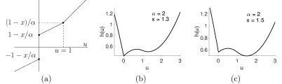
Figure 7: (a) The derivative $h^{\prime}(u)$ for $u\in(0,\infty)$ in a typical case. Note that $h^{\prime}$ is discontinuous at $0$. (b) and (c) Plots of $h(u)$ for two values of $(\alpha,x)$ that lead to case 4.

References

- [1] P. Spirtes and C. Glymour, “An Algorithm for Fast Recovery of Sparse Causal Graphs,” Social Science Computer Review, vol. 9, no. 1, pp. 62–72, 1991.
- [2] D. Heckerman, D. Geiger, and D. M. Chickering, “Learning Bayesian Networks: The Combination of Knowledge and Statistical Data,” Machine Learning, vol. 20, pp. 197–243, 1995.
- [3] J. Suzuki, “A Construction of Bayesian Networks from Databases Based on an MDL Scheme,” in Proceedings of the Ninth International Conference on Uncertainty in Artificial Intelligence, 1993.
- [4] I. Tsamardinos, L. E. Brown, and C. F. Aliferis, “The Max-Min Hill-Climbing Bayesian Network Structure Learning Algorithm,” Machine Learning, vol. 65, no. 1, pp. 31–78, 2006.
- [5] J. A. Gámez, J. L. Mateo, and J. M. Puerta, “Learning Bayesian Networks by Hill Climbing: Efficient Methods Based on Progressive Restriction of the Neighborhood,” Data Mining and Knowledge Discovery, vol. 22, pp. 106–148, 2011.
- [6] D. M. Chickering, “Optimal Structure Identification with Greedy Search,” Journal of Machine Learning Research, vol. 3, pp. 507–554, 2002.
- [7] P. Larrañaga, M. Poza, Y. Yurramendi, R. H. Murga, and C. M. H. Kuijpers, “Structure Learning of Bayesian Networks by Genetic Algorithms: A Performance Analysis of Control Parameters,” IEEE Transactions on Pattern Analysis and Machine Intelligence, vol. 18, no. 9, pp. 912–926, 1996.
- [8] M. Teyssier and D. Koller, “Ordering-Based Search: A Simple and Effective Algorithm for Learning Bayesian Networks,” in Proceedings of the 21st Conference on Uncertainty in Artificial Intelligence, 2005, pp. 584–590.
- [9] J. I. Alonso-Barba, L. delaOssa, and J. M. Puerta, “Structural Learning of Bayesian Networks Using Local Algorithms Based on the Space of Orderings,” Soft Computing, vol. 15, no. 10, pp. 1881–1895, 2011.
- [10] M. Scanagatta, C. P. de Campos, G. Corani, and M. Zaffalon, “Learning Bayesian Networks with Thousands of Variables,” in Advances in Neural Information Processing Systems, 2015, pp. 1864–1872.
- [11] M. Scanagatta, G. Corani, and M. Zaffalon, “Improved Local Search in Bayesian Networks Structure Learning,” in Proceedings of Machine Learning Research, vol. 73, 2017, pp. 45–56.
- [12] T. Silander and P. Myllymäki, “A Simple Approach for Finding the Globally Optimal Bayesian Network Structure,” in Proceedings of the 22nd Conference Annual Conference on Uncertainty in Artificial Intelligence, 2006, pp. 445–452.
- [13] M. Bartlett and J. Cussens, “Advances in Bayesian Network Learning using Integer Programming,” in Proceedings of the 29th Conference on Uncertainty in Artificial Intelligence, 2013, pp. 182–191.
- [14] C. Lee and P. van Beek, “Metaheuristics for Score-and-Search Bayesian Network Structure Learning,” in Proceedings of the 30th Canadian Conference on Artificial Intelligence, 2017, pp. 129–141.
- [15] M. Champion, V. Picheny, and M. Vignes, “Inferring Large Graphs Using -Penalized Likelihood,” Statistics and Computing, vol. 28, pp. 905–921, 2018.
- [16] N. Friedman and D. Koller, “Being Bayesian about Network Structure. A Bayesian Approach to Structure Discovery in Bayesian Networks,” Machine Learning, vol. 50, pp. 95–125, 2003.
- [17] B. Ellis and W. H. Wong, “Learning Causal Bayesian Network Structures from Experimental Data,” Journal of the American Statistical Association, vol. 103, no. 482, pp. 778–789, 2008.
- [18] G. F. Cooper and E. Herskovits, “A Bayesian Method for the Induction of Probabilistic Networks from Data,” Machine Learning, vol. 9, pp. 309–347, 1992.
- [19] D. M. Chickering, “Learning Bayesian Networks is NP-Complete,” in Learning from Data, ser. Lecture Notes in Statistics. Springer, 1996.
- [20] F. Fu and Q. Zhou, “Learning Sparse Causal Gaussian Networks with Experimental Intervention: Regularization and Coordinate Descent,” Journal of the American Statistical Association, vol. 108, pp. 288–300, 2013.
- [21] B. Aragam and Q. Zhou, “Concave Penalized Estimation of Sparse Gaussian Bayesian Networks,” Journal of Machine Learning Research, vol. 16, pp. 2273–2328, 2015.
- [22] B. Efron, T. Hastie, I. Johnstone, and R. Tibshirani, “Least Angle Regression,” The Annals of Statistics, vol. 32, no. 2, pp. 407–499, 2004.
- [23] P. Spirtes, C. Glymour, and R. Scheines, Causation, Prediction, and Search. Springer-Verlag, New York, 1993.
- [24] L. Vandenberghe and M. S. Andersen, “Chordal Graphs and Semidefinite Optimization,” Foundations and Trends in Optimization, vol. 1, no. 4, pp. 241–433, 2014.
- [25] C.-H. Zhang, “Nearly Unbiased Variable Selection under Minimax Concave Penalty,” The Annals of Statistics, vol. 38, no. 2, pp. 894–942, 2010.
- [26] J. Pearl, “Causal Diagrams for Empirical Research,” Biometrika, vol. 82, pp. 669–710, 1995.
- [27] J. Robins, “A New Approach to Causal Inference in Mortality Studies with a Sustained Exposure Period - Application to Control of the Healthy Worker Survivor Effect,” Mathematical Modelling, vol. 7, pp. 1393–1512, 1986.
- [28] N. Parikh and S. Boyd, “Proximal Algorithms,” Foundations and Trends in Optimization, vol. 1, no. 3, pp. 123–231, 2013.
- [29] G. Schwarz, “Estimating the Dimension of a Model,” The Annals of Statistics, vol. 6, no. 2, pp. 461–464, 1978.
- [30] M. Scutari. Bayesian network repository. Accessed: 2019-01-21. [Online]. Available: http://www.bnlearn.com/bnrepository/
- [31] B. Aragam, J. Gu, and Q. Zhou, “Learning Large-Scaled Bayesian Networks with the sparsebn Package,” Journal of Statistical Software, 2019, arXiv:1703.04025.
- [32] J. D. Ramsey, “Scaling up Greedy Causal Search for Continuous Variables,” arXiv:1507.07749, 2015.
- [33] M. Scutari, “Learning Bayesian Networks with the bnlearn R Package,” Journal of Statistical Software, vol. 35, no. 3, pp. 1–22, 2010.
- [34] A. Ghoshal and J. Honorio, “Learning Linear Structural Equation Models in Polynomial Time and Sample Complexity,” in Proceedings of Machine Learning Research, vol. 84, 2018, pp. 1466–1475.
- [35] A. Hauser and P. Bühlmann, “Characterization and Greedy Learning of Interventional Markov Equivalence Classes of Directed Acyclic Graphs,” The Journal of Machine Learning Research, vol. 13, pp. 2409–2464, 2012.
- [36] J. Gu, F. Fu, and Q. Zhou, “Penalized Estimation of Directed Acyclic Graphs from Discrete Data,” Statistics and Computing, vol. 29, pp. 161–176, 2019.