Probing local cosmic rays using Fermi-LAT observation of a mid-latitude region in the third Galactic quadrant

Abstract

The $\gamma$-ray observation of interstellar gas provides a unique way to probe the cosmic rays (CRs) outside the solar system. In this work, we use an updated version of Fermi-LAT data and recent multi-wavelength tracers of interstellar gas to re-analyze a mid-latitude region in the third Galactic quadrant and estimate the local CR proton spectrum. Two $\gamma$-ray production cross section models for $pp$ interaction, the commonly used one from Kamae et al. (2006) and the up-to-date one from Kafexhiu et al. (2014), are adopted separately in the analysis. Both of them can well fit the emissivity and the derived proton spectra roughly resemble the direct measurements from AMS-02 and Voyager 1, but rather different spectral parameters are indicated. A break at $4\pm 1~{}{\rm GeV}\;c^{-1}$ is shown if the cross section model by Kamae et al. (2006) is adopted. The resulting spectrum is $\lesssim 20\%$ larger than the AMS-02 observation above 15 GeV and consistent with the de-modulated spectrum within $2\%$. The proton spectrum based on the cross section model of Kafexhiu et al. (2014) is about $1.4-1.8$ times that of AMS-02 at $2-100~{}\rm GeV$, however the difference decreases to 20% below 10 GeV with respect to the de-modulated spectrum. A spectral break at $20\pm 11~{}{\rm GeV}\;c^{-1}$ is required in this model. An extrapolation down to 300 MeV is performed to compare with the observation of Voyager 1, and we find a deviation of $\lesssim 2.5\sigma$ for both the models. In general, an approximately consistent CR spectrum can be obtained using $\gamma$-ray observation nowadays, but we still need a better $\gamma$-ray production cross section model to derive the parameters accurately.

I Introduction

Cosmic rays (CRs) play a vital role in the Galactic ecosystem, because they heat and ionize the interstellar gas, and provide an additional support against the gravitational force together with the magnetic field (Ferrière, 2001; Grenier et al., 2015). Nowadays, there are some experiments aiming at collecting the CR particles, however due to the solar modulation, the intrinsic CR spectra in local interstellar space (LIS) below $\sim 10$ GeV/nuc can not be measured directly near the Earth (Gleeson and Axford, 1968). The Voyager 1 and Voyager 2 crossed the heliopause on 2012 August 25 (Stone et al., 2013) and 2018 November 5 respectively, and started to measure the CR spectra outside the heliosphere (Stone et al., 2013; Cummings et al., 2016), which are thought to be the same as the LIS ones (Kóta and Jokipii, 2014). But the LIS proton spectrum from $0.35~{}\rm GeV$ to $\sim 10~{}\rm GeV$ is still not available right now (Cummings et al., 2016).

The interaction of CRs with the interstellar gas will produce $\gamma$-ray photons. On one hand, these $\gamma$ rays can be a useful tracer of total gas column density (Lebrun et al., 1982; Grenier et al., 2005a; Ade et al., 2015; Mizuno et al., 2016; Abrahams et al., 2017; Remy et al., 2017, 2018a, 2018b), since the $\gamma$ rays are transparent to the interstellar medium (ISM) and also independent of the chemical and thermodynamic state. On the other hand, $\gamma$-ray observation provides a unique way to probe the Galactic CRs outside the solar system. Particularly, the observation of distant gas reflects the CR spectra there, which will shed light on the origin and propagation of CR or even help to find the site of CR acceleration (Aharonian, 2001; Casanova et al., 2010).

The Fermi Gamma-ray Space Telescope (Fermi) is launched on 2008 June 11, with a pair-conversion telescope, Large Area Telescope (LAT), on board (Atwood et al., 2009). Thanks to its unprecedented sensitivity and accurate calibration (Abdo et al., 2009a, b; Ackermann et al., 2012a), a plenty of researches have been done to constrain the CR spectra elsewhere in the Galaxy (Abdo et al., 2009c, 2010; Ackermann et al., 2011; Neronov et al., 2012; Ackermann et al., 2012b, c, d; Yang et al., 2014; Abrahams and Paglione, 2015; Yang et al., 2015; Tibaldo et al., 2015; Casandjian, 2015; Yang et al., 2016; Acero et al., 2016; Neronov et al., 2017; Shen et al., 2018; Aharonian et al., 2018). Interstellar gas in the mid-Galactic latitude region is a favorable target to study the LIS CRs, because the gas there is mostly not far from the sun (Abdo et al., 2009c). The first $\gamma$-ray analysis of local H i gas in Fermi era is performed in Abdo et al. (2009c) and it is found to be consistent with the Galprop prediction. Further efforts aim at deriving the LIS CR spectra using the $\gamma$-ray observation of all mid-Galactic regions down to 60 MeV (Casandjian, 2015; Strong, 2016). The results are quite close to the PAMELA spectrum after the solar modulation correction, when the systematic uncertainties are considered. Giant molecular clouds (GMCs) in the Gould Belt are also adopted to probe the LIS CR, because these clouds are nearby and bright in $\gamma$-ray sky. Some nearby GMCs have been analyzed Neronov et al. (2012); Yang et al. (2014); Neronov et al. (2017) and their emissivities are found to be similar, suggesting the $\gamma$-ray emission is mainly from the passive interaction with the Galactic CR sea which is also confirmed in (Ackermann et al., 2012c; Peng et al., 2019). The CR spectrum can therefore be obtained with the emissivities of $\rm H_{2}$, however point source contamination might be a problem in the low energy range due to their relatively small size (Yang et al., 2014).

Over the last few years, the quality of Fermi-LAT data has been improved, which not only provides a larger effective area particularly in the lower energy range, but also reduces the instrumental systematic uncertainties (Atwood et al., 2013). New multi-wavelength observations of ISM are available, e.g. the H i survey from Ben Bekhti et al. (2016), the dust opacity and extinction from (Aghanim et al., 2016; Ade et al., 2016a). Furthermore, the $\gamma$-ray production cross section model for $pp$ interaction is updated in Kafexhiu et al. (2014). Taking advantage of the updated observations and tools, we revisit the analysis of a mid-Galactic latitude region in the third quadrant which has be done in Abdo et al. (2009c). We choose this region because local atomic hydrogen dominates the gas column density in it (Abdo et al., 2009b), which enables us to directly calculate the number of atoms along the line of sight and therefore is less prone to the uncertainty of the dark gas and CO-to-$\rm H_{2}$ conversion factor. Comparing to the previous work in (Casandjian, 2015), we perform our analysis in a relatively clean region, use the updated ISM tracers to estimate the gas column density and more complete Fermi-LAT 8-year source catalog to reduce the point source contamination.

In this paper, data reduction, including the template generation and the analysis procedure, is described in Sec. II. In the Sec. III, the $\gamma$-ray spectrum and its systematic uncertainty are presented. We then extract the LIS proton spectrum using either the latest cross section model from Kafexhiu et al. (2014) or the popular one from Kamae et al. (2006), and compare them with the direct measurements of AMS-02 (Aguilar et al., 2015) and Voyager 1 (Cummings et al., 2016). Finally, a summary is given in Sec. IV.

II Data analysis

II.1 $\gamma$-ray data

The Fermi-LAT P8R3 data, based on the most recent iteration of the event-level analysis, are released recently. In this data version, the leak of charged particles through the scintillating ribbons is removed, and therefore the anisotropy problem of the background model in the previous version is solved (Bruel et al., 2018). We choose the Clean event class of P8R3 data. By using this data set, we can suppress the residual CR background at a reasonable cost of data. Photons observed from 2008 August 4 to 2018 November 22 (Fermi Mission Elapsed Time (MET) from 239557417 to 564539821) with energy between 75 MeV and 100 GeV are selected. We further exclude the reconstructed zenith angles over 85^∘ to reduce the contamination from the Earth’s limb, and then apply the recommended quality-filter cut $\rm(DATA\_QUAL>0)\&\&(LAT\_CONFIG==1)$, which removes the events collected outside science mode or during the time interval when either a solar flare or particle event happens. The events between July 14 and September 13 in each year are also excluded in order to remove the emission from the Sun in the region of interest (ROI) defined below.

We choose a rectangular area in the carrée projection centering at $(l,b)=(230^{\circ},41^{\circ})$ as our ROI. The photons in the ROI are partitioned into $240\times 152$ pixels with the bin size of 0.25^∘, as shown in the Fig. 1, and 25 logarithmically spaced energy bins to build a count cube.

Throughout this work, fermitools v1.0.0, the latest toolkit for Fermi-LAT data analysis, is used.

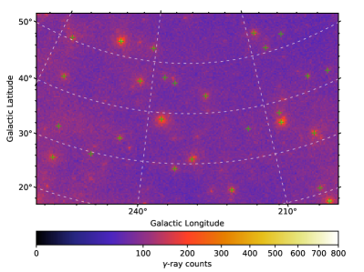
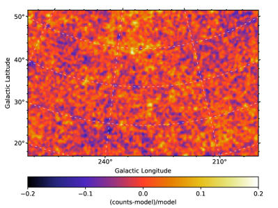
Figure 1: Count map (left) for $\gamma$ rays from 75 MeV to 100 GeV and residual map (right) showing the difference between the observed and modeled counts divided by the expected count map. The bright point sources which are fitted separately are marked as green crosses in the count map. The residual map is smoothed with a $1^{\circ}$ Gaussian kernel to reduce statistical fluctuation.

II.2 Components of the Galactic diffuse emission

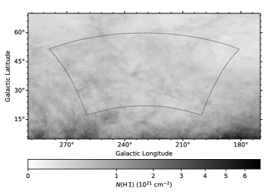
Figure 2: The H i column density in the source region. The spin temperature is assumed to be 125 K. The dashed line encloses the ROI of our analysis.

Galactic $\gamma$-ray diffuse emission originates from the interaction of CRs with interstellar gas and radiation field. The decay of $\pi^{0}$ mesons and the electron bremsstrahlung are responsible for the former component, while the inverse Compton (IC) process contributes to the latter one. Since all the diffuse emissions are merged into a single interstellar emission model gll_iem_v06.fits (Acero et al., 2016), we need to replace it with its composition to derive the $\gamma$-ray spectrum associated with H i. The main procedure of making each component is very similar to Shen et al. (2018) and will be described in the following. To take into account the photons reconstructed inside the ROI but originated from sources outside, we define $170^{\circ}\leq l\leq 290^{\circ}$, $5^{\circ}\leq b\leq 70^{\circ}$ as our source region (SR), within which we make the templates.

The atomic hydrogen contributes to the majority of the gas in the SR (Abdo et al., 2009c). We use the 21-cm hyperfine structure line data provided by the H i $4\pi$ survey (HI4PI) (Ben Bekhti et al., 2016), as it provides a better angular resolution compared to its predecessor (Kalberla et al., 2005). Even though HI4PI covers a wide local standard of rest (LSR) velocity range from $-600~{}\rm km\;s^{-1}$ to $600~{}\rm km\;s^{-1}$, we exclude the data with $|v_{\rm LSR}|\geq 70~{}\rm km\;s^{-1}$ following Abergel et al. (2014) to eliminate the H i emission from high-velocity clouds (HVCs) and extra-Galactic objects within our SR (Westmeier, 2018), concerning no dust thermal emission (Wakker and van Woerden, 1997) or $\gamma$-ray emission Tibaldo et al. (2015) of HVC has been found. To calculate the H i column density $N(\rm{H\,\textsc{i}})$, we assume the spin temperature $T_{\rm S}=125~{}\rm K$ in our baseline model Abdo et al. (2009c), and will try other $T_{\rm S}$ during the evaluation of systematic uncertainties. The final $N(\rm{H\,\textsc{i}})$ map is shown in Fig. 2.

Although our ROI is chosen to exclude bright molecular clouds, there are still some CO emissions at the edge of the SR. These clouds might influence our results in the lowest energy range due to the poor angular resolution. The CO lines observed by the CfA telescope (Dame et al., 2001) and optimized with moment masking method (Dame, 2011) are used in this work. We integrate the CO brightness temperature in the SR to construct the $W_{\rm CO}$ map. The pixels sampled at 0.25^∘ are linearly interpolated to 0.125^∘ (Abdo et al., 2010). We notice that CfA survey only observes the CO emission at $|b|<32^{\circ}$, which does not cover all of the SR, however the completeness is proven with the emission from dust and H i (Dame et al., 2001). We also do not find significant CO clouds appear in the Planck TYPE 1 CO map Ade et al. (2014) but are unobserved by CfA survey in our SR.

Ionized gas is also a component of the interstellar gas with a typical volume-averaged free electron density $n\approx 0.01-0.1~{}\rm cm^{-3}$. Since the diffuse warm ionized gas is 8 times more extended in scale height than H i (Gaensler et al., 2008), it will contribute to the gas column density in the SR. Based on the Planck emission measure map in Ade et al. (2016b), we adopt the method detailed in Westerhout (1958); Ackermann et al. (2012b) and the effective electron density $n_{\rm eff}=2~{}\rm cm^{-3}$ (Sodroski et al., 1997) to make H ii column density N(H ii).

Other than the gas of different phases directly traced by multi-wavelength observations, a missing component still exists in the total gas column density derived from dust thermal emission and $\gamma$ rays (Grenier et al., 2005a). This extra component, known as the dark neutral medium (DNM), consists of the optically thick H i and the $\rm H_{2}$ without CO emission (Grenier et al., 2005a; Ade et al., 2011; Murray et al., 2018). Despite little CO emission is observed in SR, it is still possible that DNM exists. We choose the latest 353 GHz dust opacity map (Aghanim et al., 2016) as our dust tracer template $D(l,b)$ and derive the DNM template using the iterative method described below. We first make an initial DNM map with all pixels being zero. Then a linear combination of gas and DNM templates is calculated as the expected total gas column density, i.e.

$$M(l,b) = D_{\rm DNM,prev}+y_{\rm{H\,\textsc{i}}}\left[N({\rm{H\,\textsc{i}}})+X_{\rm CO}W_{\rm CO}\right]$$ (1)

$$+ y_{\rm{H\,\textsc{ii}}}N({\rm{H\,\textsc{ii}}})+y_{\rm iso},$$

where $D_{\rm DNM,prev}$ represents the DNM map derived from previous iteration and $y_{\rm iso}$ is introduced to account for the residual noise and the uncertainty of dust map in the zero level (Abergel et al., 2014). The expected total density is fitted against the 353 GHz opacity map which minimizes the difference govern by

$$\chi_{\rm dust}^{2}=\sum_{l,b}\frac{\left[D(l,b)-M(l,b)\right]^{2}}{\sigma^{2}(l,b)},$$ (2)

where $\sigma(l,b)$ is defined to be proportional to $D(l,b)$ Ade et al. (2015); Tibaldo et al. (2015); Remy et al. (2017). Considering no CO emission appears in the ROI, we simply add the H i and CO together with a fixed CO-to-$\rm H_{2}$ conversion factor $X_{\rm CO}=0.9\times 10^{20}~{}\rm K\;\rm km\;s^{-1}$ (Casandjian, 2015) in eq.(1) to make the fitting easier to converge. After the optimization, the excess with more than $3\sigma$ deviation from the core of the residual map distribution is extracted as the new DNM template for the next iteration. The fitting and extraction procedure continue until the $\chi^{2}$ in eq.(2) stabilizes, and the $D_{\rm DNM}$ in the last iteration is our final template.

The final part in the Galactic diffuse model is the IC radiation. We adopt the same IC model as the one in the standard Fermi-LAT Galactic model (Acero et al., 2016), which is calculated with the CR propagation code Galprop (Strong and Moskalenko, 1998; Strong et al., 2000; Porter et al., 2008) using the parameter set named as ${\rm{}^{S}Y^{Z}6^{R}30^{T}150^{C}2}$ (Ackermann et al., 2012e). Different IC models will also be analyzed as we evaluate the systematic uncertainties.

Loop I is a circle-like structure with a diameter of $\sim 100^{\circ}$. It was discovered in a survey of radio continuum (Large et al., 1962) and is also visible in the $\gamma$-ray band (Grenier et al., 2005b; Casandjian et al., 2009). Although its $\gamma$-ray emission is contributed by the IC process as well, it is not contained in the Galprop IC model. We include the Loop I in our analysis since it locates on the edge of our ROI. We adopt a geometrical model Wolleben (2007) using the parameters from (Ackermann et al., 2014) as our Loop I template.

II.3 $\gamma$-ray analysis procedure

Instead of adopting the correlation-based method in Abdo et al. (2009c), we follow the well developed analysis scheme assuming the gas is transparent to $\gamma$ rays (Lebrun et al., 1983; Strong et al., 1988; Digel et al., 1996; Grenier et al., 2005a; Abdo et al., 2010; Casandjian, 2015). The $\gamma$-ray intensity $I_{\gamma}$ in the direction of $(l,b)$ at the energy $E$ is given by

$$I_{\gamma}(l,b,E) = q_{\rm\rm{H\,\textsc{i}}}(E)\,\left[N({\rm{H\,\textsc{i}}})(l,b)+X_{\rm CO}\,W_{\rm CO}(l,b)\right]$$ (3)

$$+ q_{\rm\rm{H\,\textsc{ii}}}(E)\,N({\rm{H\,\textsc{ii}}})(l,b)+q_{\rm DNM}(E)\,D_{\rm DNM}(l,b)$$

$$+ x_{\rm IC}(E)\,I_{\rm IC}(l,b,E)+x_{\rm LoopI}(E)\,I_{\rm LoopI}(l,b)$$

$$+ x_{\rm iso}(E)\,I_{\rm iso}(E)$$

$$+ x_{\rm ps}(E)\,\sum_{j=1}^{n_{\rm ps,nf}}S_{j}(E)\,\delta(l-l_{j},b-b_{j})$$

$$+ \sum_{k=1}^{n_{\rm ps,f}}S_{k}(E;\theta_{k})\,\delta(l-l_{k},b-b_{k}),$$

where $q$ stands for the $\gamma$-ray emissivity of the corresponding gas, and scaling factor $x$ is intended to fine tune the spectrum given in the map cube model. Since no CO emission in the ROI, we combine the $W_{\rm CO}$ with the H i column density using a fixed factor $X_{\rm CO}=0.9\times 10^{20}~{}\rm K\;\rm km\;s^{-1}$ (Casandjian, 2015). $I_{\rm iso}$ is the intensity of the isotropic background tabulated in iso_P8R3_CLEAN_V2.txt. The sources inside the SR listed in the Fermi-LAT 8-year point source list (FL8Y) are included, with the bright ones shown in Fig. 1. The spectrum for each source is $S(E;\theta)$ with the parameters being $\theta$. To limit the number of free parameters, sources with statistical significance smaller than 25 are merged into a single template based on the parameters given in the catalog and the others are left as individual templates. The number of point sources with spectral parameters freed is $n_{\rm ps,f}$ and the number of the remaining is $n_{\rm ps,nf}$.

The expected $\gamma$-ray intensity given above is convolved with the Fermi-LAT instrumental response functions (IRFs) with the gtsrcmaps, and the binned likelihood fitting is performed using the pyLikelihood (Mattox et al., 1996; James and Roos, 1975). Since the uncertainty of the energy measurement will distort spectral parameters especially in the lower energy range, we take the energy dispersion correction into account for all the $\gamma$-ray emitting components except the isotropic background.

We first perform a global fit before the bin-by-bin analysis, which helps to alleviate the overfitting problem and make the energy dispersion correction more accurate. In the global fit, we choose the LogParabola spectral type for all the emissivities of gas, and optimize both the normalizations and the spectral indexes. Because the spectral shape and spatial map of the IC emission are related to the CR electron distribution in the Milky Way, we only fit its normalization. The intensity of the standard isotropic background is derived based on the standard Galactic interstellar model (Acero et al., 2016), so instead of just varying its prefactor in the fitting, we adopt a PowerLaw scaling factor to adjust the spectral index as well. We set free normalizations of FL8Y sources with significance larger than 25. The spectral shapes of the sources $\geq 35\sigma$ are also fitted. Concerning the sources merged into a single template, we adopt a PowerLaw scaling factor to tune their prefactors and indexes as a whole.

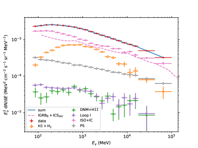
Figure 3: The intensity spectra for the observed counts and the components for our ROI in the baseline model. The uncertainties of the counts are only statistical, while the error bars of each component are obtained from the fittings. The pink dashed line shows the isotropic diffuse $\gamma$-ray background (IGRB) model B in Ackermann et al. (2015) plus the IC spectrum from ${\rm{}^{S}Y^{Z}6^{R}30^{T}150^{C}2}$ model.

A bin-by-bin fitting is performed based on the resultant model in the global fit. Since the inference in high energy range suffers from low statistics, we treat the six highest energy bins as two bins and fit three of them each time. All the spectral indexes are kept fixed during the optimization. Furthermore, we replace the indexes of DNM and H ii with that of H i, because the first two are much weaker than H i and their emissivities should have the same shape as H i. The normalization of IC model is also frozen to reduce the correlation with the isotropic background.

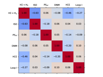
Figure 4: The correlation matrix between the normalizations of different large scale components in the baseline model derived in the global fitting. The $\rm PS_{nf}$ represents the single template for the weak point sources. We do not present the correlations of strong point sources, since they are fitted as individual point sources and are seldom correlated with the diffuse components.

Before presenting the results, we will first do some fit quality checks. Based on the best-fit parameters in each energy bin, we make a residual map (right panel of Fig. 1) and average intensities of different $\gamma$-ray emitting components (Fig. 3). To obtain the residual map, we subtract the sum of best-fit models in each energy bin from the observed count map, and then divide it by the predicted map. The maps are smoothed with $1^{\circ}$ Gaussian kernel to reduce the statistical fluctuation. We do not find any significant structure in the residual map, with the minimum and maximum deviation being $-0.15$ and $0.17$ respectively. In the intensity map, we adopted the average intensity of each component in the ROI along with its uncertainty obtained from the fittings. We combine the spectra of isotropic and IC components since both of them are structureless in the ROI. We also add the intensities of DNM and H ii together, considering that they are not as significant as other components and should have a similar spectral shape. The uncertainty of the combined components is calculated by summing quadratically the errors of individual contributions. The spectrum of observed counts and its statistical uncertainty in the figure are also given. As shown in the figure, the model can well describe the observed count spectrum. Since the H i gas is anti-correlated with some of the diffuse components, isotropic background in particular, as depicted in Fig. 4, the uncertainty of H i gas spectrum is larger than Poisson ones. Our $\rm ISO+IC$ intensity is larger than the isotropic diffuse $\gamma$-ray background (IGRB) model B in Ackermann et al. (2015) plus the IC spectrum from ${\rm{}^{S}Y^{Z}6^{R}30^{T}150^{C}2}$ model (pink dashed line) by around $\sim 10\%-50\%$. It might be explained by residual CR background and and the different IC models adopted in this work from Ackermann et al. (2015).

III Results and Discussion

III.1 Results of the baseline model and the systematic uncertainties

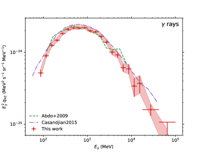
Figure 5: $\gamma$-ray emissivity per H i atom in the baseline model and its uncertainty. The red points and error bars indicate the best-fit values and $1\sigma$ statistical uncertainties in the baseline model. 95% upper limits are given when the TS value in that energy bin is smaller than 10. The red band shows the total errors including both the statistical and systematic uncertainties. The green dashed line and purple dot-dashed line illustrate the emissivity in (Abdo et al., 2009c) and (Casandjian, 2015), respectively.

The $\gamma$-ray emissivity per H i atom in each energy bin is obtained using the best-fit spectral parameters, which is illustrated in Fig. 5. The integral emissivities above 75 MeV and 100 MeV are $(1.63\pm 0.08)\times 10^{-26}~{}\rm ph\;s^{-1}\;sr^{-1}$ and $(1.46\pm 0.06)\times 10^{-26}~{}\rm ph\;s^{-1}\;sr^{-1}$ respectively. Comparing with Abdo et al. (2009c) (green dashed line), which adopted a similar ROI to ours, spectral shape is similar but the integral is smaller, which might be caused by the updated background and templates. Our emissivity is also consistent with Casandjian (2015) (purple dot-dashed line), which uses a larger ROI but older $\gamma$-ray data and gas tracers.

The $\gamma$-ray emissivity above is based on the templates described in Sec. II.2 and the standard Fermi-LAT IRFs. In order to investigate the systematic uncertainties associated with them, we substitute the $\gamma$-ray emitting templates and also propagate the uncertainty on effective area in the following. During the evaluation, the data analysis procedure is the same as that given in Sec. II.3.

A uniform spin temperature $T_{\rm S}=125~{}\rm K$ is used in the baseline model to convert the brightness temperature into the H i column density. A higher $T_{\rm S}$ means more electrons in hydrogen atoms are in the higher energy spin state, thus less absorption is experienced and smaller column density is expected. We try three different $T_{\rm S}$ values 100 K, 200 K and $\infty$ K, which will decrease the H i column density by $-1.5\%$, 2.1% and 5.3% on average respectively. This type of uncertainty causes the emissivity to shift between $\sim-2\%$ and $\sim 8\%$.

The IC model is calculated based on a specific propagation parameters with Galprop (Acero et al., 2016). Different parameters will lead to different spectral and spatial shapes, and thus affect the emissivity. We vary the IC model by using different Galprop parameter sets (Ackermann et al., 2012e; de Palma et al., 2013), whose identifications are ${\rm{}^{S}L^{Z}4^{R}20^{T}150^{C}2}$, ${\rm{}^{S}L^{Z}10^{R}30^{T}\infty^{C}5}$, ${\rm{}^{S}S^{Z}4^{R}20^{T}150^{C}2}$, and ${\rm{}^{S}S^{Z}10^{R}30^{T}\infty^{C}5}$. The IC templates only affect the emissivity in the high energy range, which leads to at most 2% difference above $\sim 50~{}\rm GeV$.

The uncertainty of the effective area ($A_{\rm eff}$) dominates the instrument-related systematic uncertainties. In our case, the largest relative uncertainty is 10% at 31.6 MeV, decreases to 3% at 100 MeV, stays at 3% until 100 GeV, and then increases to 15% at 1 TeV. We use the bracketing $A_{\rm eff}$ method to propagate the uncertainty to the spectral parameters. To investigate the largest influence, we replace the $A_{\rm eff}$ with the upper and lower bound of the uncertainty for the sources with spectral indexes freed except the isotropic background and the merged template for weak sources. It results in a $3\%-5\%$ change of the emissivity.

The total uncertainty including the statistical and systematic uncertainty is calculated with their root sum square, and is shown as a red band in Fig. 5.

III.2 LIS CR spectrum

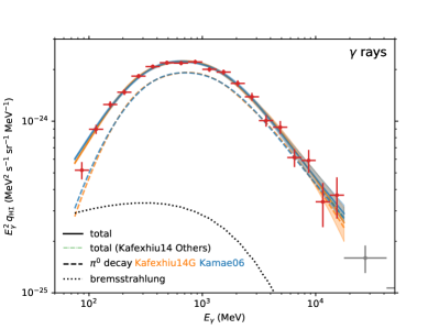
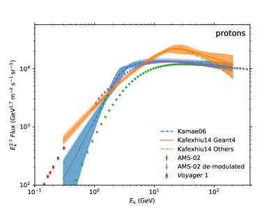
Figure 6: The $\gamma$-ray emissivity of H i in the baseline model along with the best-fit $\gamma$-ray (left) and proton spectra (right). The data used in the fittings are drawn as red points and the others as gray ones. The results based on the cross section model from Kafexhiu et al. (2014) and Kamae et al. (2006) are shown in orange and blue respectively. Only the statistical uncertainty of the baseline model is shown in left-hand figure. While in the right panel, the statistical and total errors are drawn with the dark and light color bands respectively. The extrapolated proton spectra are plot in dotted lines. The measurement from Voyager 1 (Cummings et al., 2016) and AMS-02 (Aguilar et al., 2015) are shown in red squares and green dots, while the de-modulated AMS-02 flux is shown in purple triangles. We also show the results using the parameterizations other than the EXPERIMENT+GEANT4 one with green dot-dashed lines in both figures.

Since the $\gamma$-ray emissivity of interstellar gas comes from the $\pi^{0}$ decay and bremsstrahlung, a model consisting of the two emission processes is needed to fit the $\gamma$-ray observation and derive the CR spectrum.

The $\gamma$-ray production cross section in the $pp$ collisions is updated in Kafexhiu et al. (2014). It takes advantage of the published experimental data for the proton kinetic energy below 2 GeV and some sophisticated Monte Carlo codes in the higher energy. We adopt the cross section parameterization EXPERIMENT+GEANT4 to account for the $\gamma$-ray emission from the process. Since the interaction between a proton and a heavier nucleus may also produce $\gamma$-ray photons, we scale the cross section with an energy-dependent enhancement factor as in Kafexhiu et al. (2014). Because of the large systematic uncertainty of the cross section model, we also employ the widely-used cross section from Kamae et al. (2006) and an enhancement factor of 1.78 (Casandjian, 2015) as an alternative. To avoid being cumbersome in the following, we define the $\gamma$-ray model containing the former cross section as KA14 model and containing the latter one as KK06 model. The CR protons are assumed to follow a smoothly broken power law spectral shape (Strong, 2016), i.e.

$${\rm d}F/{\rm d}p=A\,(p/p_{0})^{-\alpha_{1}}\,[1+(p/p_{\rm br})^{(\alpha_{2}-\alpha_{1})/\beta}]^{-\beta},$$ (4)

where $p$ is the momentum of a proton and $p_{0}$ is fixed to $3~{}{\rm GeV}\;c^{-1}$. The normalization $A$, spectral indexes $\alpha_{1}$, $\alpha_{2}$ and break momentum $p_{\rm br}$ will be optimized and the smoothness factor $\beta$ will be fixed to 0.2.

As to the bremsstrahlung emission, the cross section from Strong et al. (2000) is employed. We also include the bremsstrahlung emission from the CR electrons and positrons scattered by the heliums, which is a factor of 0.096 the abundance of hydrogen in the local ISM (Meyer, 1985). Since the bremsstrahlung is the subdominant component in our energy range, we simply use the all-electron spectrum for PDDE model in Orlando (2018), which is well fitted to the directly measured electron spectrum and some synchrotron observations between 40 MHz and 20 GHz.

We fit CR proton spectrum using the $\gamma$-ray emissivity of baseline model below 17.8 GeV. The data in the higher energy range are excluded due to the low statistics. The best-fit $\gamma$-ray models and the resultant proton spectra based on the two cross sections are shown in Fig. 6. Because the $\gamma$-ray data are only from 75 MeV, proton spectrum below $\sim 900~{}\rm MeV$ is not directly constrained by $\gamma$-ray emissivity (Kafexhiu et al., 2014). An extrapolation down to the kinetic energy of 300 MeV is performed based on the best-fit models and is indicated with dotted lines in the right panel. The statistical uncertainty of the proton spectra is shown in dark shaded regions, and the total errors including the systematic uncertainty propagated from the $\gamma$-ray emissivity is given with the light color band. To compare with the direct CR observations, we plot the proton measurements from AMS-02 (Aguilar et al., 2015) and Voyager 1 (Cummings et al., 2016) with green dots and red squares respectively. Also drawn in purple triangles is the de-modulated AMS-02 proton flux. To derive the solar modulation potential, the non-parametric method in Zhu et al. (2018) is adopted. We assume a spline interpolation of LIS proton spectrum and fit the proton spectra with and without correction to the AMS-02 and Voyager 1 measurements. It results in a potential of $\phi=0.57\pm 0.04~{}\rm GV$.

The KK06 model gives a reasonable fit to the baseline emissivity, with the $\chi^{2}/$dof being 18.3/15. The best-fit parameters of the proton spectrum are $A=(6.9\pm 2.0)\times 10^{2}\ {\rm m^{-2}\;s^{-1}\;sr^{-1}\;(GeV}\;c^{-1})^{-1}$, $\alpha_{1}=0.9\pm 1.0$, $\alpha_{2}=2.85\pm 0.07$, and $p_{\rm br}=4\pm 1~{}{\rm GeV}\;c^{-1}$. We find the spectral index after break matches that of AMS-02 between 45 GV and 336 GV, which is $2.849\pm 0.002$. This model provides a consistent proton spectrum with that observed by AMS-02 in the energy range where the solar modulation does not have strong impact. The maximum deviation is $\lesssim 20\%$ above 15 GeV. When we compare the result with the de-modulated proton spectrum, the difference drops to $2\%$ above 10 GeV which can be explained by the statistical and systematic uncertainties. A break at $\sim 4~{}\rm GeV$ in the best-fit model is also visible in the de-modulated spectrum. At the energy of $\sim 300$ MeV, the Voyager 1 measurement is approximately 3 times the value of the extrapolated one, corresponding to a $\sim 2.5\sigma$ deviation considering the uncertainties of the spectral parameters. This difference can be statistical or caused by the uncertainty of the cross section. If the first case is true, it suggests no strong modulation in the local ISM (Stone et al., 2013).

The KA14 model can explain the $\gamma$-ray observation as well, whose $\chi^{2}/$dof is 16.6/15 and the parameters are $A=(5.5\pm 0.1)\times 10^{2}\ {\rm m^{-2}\;s^{-1}\;sr^{-1}\;(GeV}\;c^{-1})^{-1}$, $\alpha_{1}=2.20\pm 0.08$, $\alpha_{2}=3.1\pm 0.3$, and $p_{\rm br}=20\pm 11~{}{\rm GeV}\;c^{-1}$. The best-fit spectrum has different shape from the direct measurement above 10 GeV, which is also found in Neronov et al. (2017). But concerning the large statistical errors in the break energy and the high-energy break, a spectral shape may still be consistent with the AMS-02 observation. The predicted proton flux is approximately $1.4-1.8$ times the data of AMS-02 at $2-100~{}\rm GeV$ with the maximum deviation shown at the break energy. The difference decreases to 18% at $\sim 180~{}\rm GeV$. We also try the other $pp$ collision cross-section parameterizations given in Kafexhiu et al. (2014), which are mainly different from the EXPERIMENT+GEANT4 one when the kinetic energy of proton is larger than 50 GeV, and find that their predictions are even softer after break and still can not solve the current problem (shown in green dotted-dashed lines in Fig. 6). When compared with the de-modulated spectrum below 10 GeV, the difference decreases to at most 20%. The extrapolation exceeds the measurement of Voyager 1 by $\sim 40\%$ at 300 MeV, which is $\sim 2\sigma$ larger. If it is the case, either a mild bending below $\sim 900~{}\rm MeV$ is needed or the CR in the local ISM is slightly more than that observed by Voyager 1.

IV Summary

The $\gamma$-ray observation can be used to derive the $\gamma$-ray emissivity of interstellar gas and thereby the CR spectrum. We choose a mid-latitude Galactic region as our ROI in this work to investigate the LIS CR spectrum. Using the recent version of Fermi-LAT data (Bruel et al., 2018), most complete point source catalog as well as the up-to-date multi-wavelength survey of interstellar gas (Ben Bekhti et al., 2016; Aghanim et al., 2016), we obtained the $\gamma$-ray emissivity of H i gas and its systematic uncertainties, which are illustrated in Fig. 5. Then two $\gamma$-ray production cross sections of $pp$ interaction, the commonly used one from Kamae et al. (2006) and the up-to-date one from Kafexhiu et al. (2014), are adopted to convert the emissivity into the CR spectrum.

Even though the two models can both provide reasonable fits to the data, they yield different proton spectra. The discrepancy between the spectra is $\lesssim 50\%$. It suggests a significant influence of cross section on reconstructing the proton spectrum.

The KK06 model gives a spectrum rather consistent with the AMS-02 measurement but smaller than the Voyager 1 measurement. The spectral index above the break is $2.85\pm 0.07$, which is consistent with the result from AMS-02 (Aguilar et al., 2015). There is $\lesssim 20\%$ deviation between the predicted spectrum and the AMS-02 measurement above 15 GeV, and the difference becomes as small as $2\%$ if we compare the prediction with the de-modulated data. A break at $p=4\pm 1~{}{\rm GeV}\;c^{-1}$ shown in our result is also visible in the de-modulated spectrum. An index of $0.9\pm 1.0$ is predicted in the low energy range. If an extrapolation is performed down to $\sim 300~{}\rm MeV$, the proton flux is only about 33% of the Voyager 1 measurement (Cummings et al., 2016), corresponding to a $\sim 2.5\sigma$ deviation.

The KA14 model yields a spectrum that deviates from the direct measurement in high energy (see also Neronov et al. (2017)). Specifically, about $1.4-1.8$ times the amount of directly measured protons are required between 2 GeV and 100 GeV. The difference becomes $\lesssim 20\%$ below 10 GeV when it is compared with the de-modulated spectrum. A break at $20\pm 11~{}{\rm GeV}\;c^{-1}$ is needed, with the indexes before and after the break being $2.20\pm 0.08$ and $3.1\pm 0.3$, respectively. The extrapolation exceeds the Voyager 1 measurement by $\sim 40\%$ at $\sim 300~{}\rm MeV$.

Nowadays, based on the $\gamma$-ray observation, a CR spectrum roughly resembling the direct measurement can be obtained, however the systematic uncertainty on the cross section (also shown in Casandjian (2015)) still prevents us from accurately determining the spectral parameters of CR protons. The situation is expected to change once a more accurate cross section model is available.