The annihilation number does not bound the -domination number from the above
Abstract
The -domination number of a graph is the minimum cardinality of a set such that every vertex from is adjacent to at least two vertices in . The annihilation number is the largest integer such that the sum of the first terms of the non-decreasing degree sequence of is at most the number of its edges. It was conjectured that holds for every connected graph . The conjecture was earlier confirmed, in particular, for graphs of minimum degree , for trees, and for block graphs. In this paper, we disprove the conjecture by proving that the -domination number can be arbitrarily larger than the annihilation number. On the positive side we prove the conjectured bound for a large subclass of bipartite, connected cacti, thus generalizing a result of Jakovac from [Discrete Appl. Math. 260 (2019) 178–187].
Keywords: -dominating set; -domination number; annihilation number; cactus graph
AMS Math. Subj. Class. (2010): 05C69, 05C07
1 Introduction
Let be the degree ordering of a graph . The annihilation number is the largest integer such that . This concept was first defined in [17], see also [11] for an earlier, closely related concept called Havel-Hakimi process. The -domination number of a graph is the minimum cardinality of a set such that every vertex from is adjacent to at least two vertices in . Now, the following conjecture relating these two concepts was posed.
If , then Caro and Roddity [5, Corollary 2] deduced from their main result that . Hence, holds for any graph with . Desormeaux, Henning, Rall, and Yeo [9] followed with a confirmation of the conjecture for trees (see also [16] for another proof of it). Moreover, they have also characterized the trees that attain the equality in the conjecture. Very recently, Jakovac [14] proved the conjecture for block graphs. In addition he proved:
Proposition 1.2 ([14])
If is a bipartite cactus such that every edge of belongs to a cycle, then .
In Section 2 we disprove Conjecture 1.1 by a subclass of connected cactus graphs with minimum degree . The construction further shows that the gap between the -domination number and the annihilation number can be arbitrarily large. Although the conjecture is wrong, it is still interesting to find classes of graphs which satisfy the conjecture. In Section 3 we prove several lemmas needed in the subsequent section. Then, in Section 4, we show that Conjecture 1.1 holds for bipartite connected cacti which (i) contain no sun at an outer cycle and (ii) the degree of the exit vertex of any outer -cycle is at least . (A sun at a cycle is obtained from the cycle by adding a pendant vertex to each of its vertices except one.) In this way we generalize Proposition 1.2. We conclude the paper with some open problems while in the rest of this section definitions and concepts needed are given.
1.1 Preliminaries
All graphs in this paper are undirected, finite and simple. We follow [1] for graph theoretical notation and terminology not defined here.
If is a graph, then set and . A graph is nontrivial if . For , the set of its neighbors is denoted by and called the neighborhood of , and the closed neighborhood of is . The degree of a vertex is denoted by . For a subset , we define . In the above notation we may omit the index provided that is clear from the context. A vertex of degree is a leaf while its only neighbor is called a support vertex. If has at least two neighbors which are leaves, then is referred to as a strong support vertex. The minimum and the maximum degree among the vertices of are denoted by and , respectively. If , then denotes the graph obtained from by deleting the vertices in and all edges incident with them. Moreover, if and , notations and will be used for the graph and , respectively. These and notations will also be used for sets of edges. A connected graph is a cactus if its cycles are pairwise edge-disjoint.
A vertex dominates the vertices contained in . A set is a dominating set if each vertex of is dominated or equivalently, if , where is the closed neighborhood of . The domination number is the minimum cardinality of a dominating set of . For , a -dominating set of a graph is a set such that each vertex from is adjacent to at least vertices in . There always exists at least one -dominating set in , since is clearly a -dominating set. The -domination number of is the minimum cardinality of a -dominating set of . Thus, a -dominating set is a usual dominating set and hence . The notion of the -dominating set was introduced by Fink and Jacobson [10], a survey on it up to 2012 can be found in [4]. It has been further investigated afterwards, [6, 15] are a couple of recent papers. In this paper we focus on the -domination number, cf. [3].
is an annihilation set of if and is an optimal annihilation set if . Obviously, any optimal annihilation set of a connected graph of order at least vertices contains all leaves. Assuming that is an optimal annihilation set, we denote by the minimum vertex degree over the set .
2 Counterexample to Conjecture 1.1
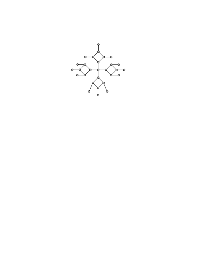
Let and . Then the graph is obtained in the following way. First, take a disjoint union of cycles , , add an additional vertex , and connect with an arbitrary but fixed vertex in each of the cycles. Second, in the so far constructed graph, add a pendant vertex to each of the vertices of degree . In Fig. 1 the graph is drawn.
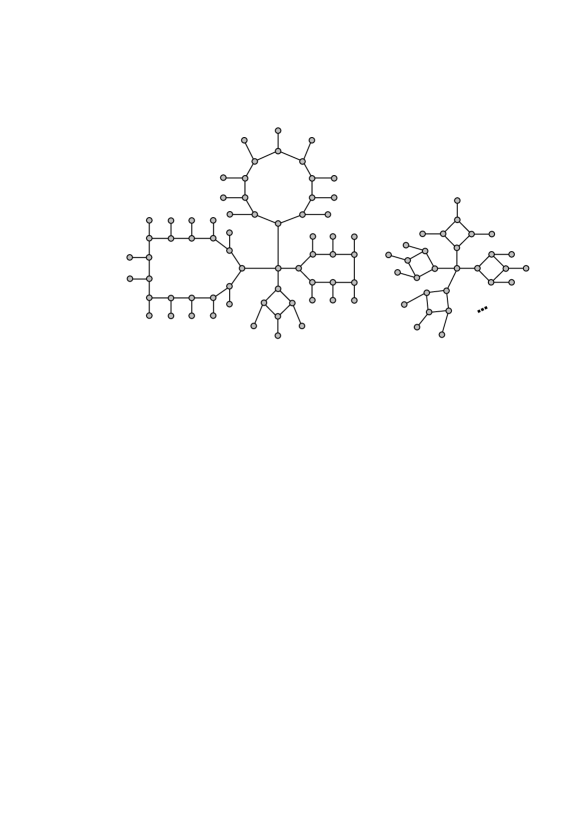
Consider first the sporadic counterexamples as shown in Fig. 2. It is straightforward to verify that and . Hence . Similarly, in the second example we have and . Therefore, .
The above examples generalize as follows.
Theorem 2.1
Let be a given positive integer, , and . If , then
Proof.
To shorten the presentation, set for the rest of the proof. Since to each of the constitutional cycles of exactly leaves are attached, as well as the edge to the vertex of degree , we get
Hence, since each leaf of is a member of its every optimal annihilation set and all the other vertices of such a set are of degree , we get
| (1) |
We now claim that . Let be a -dominating set of with . Then every leaf of lies in . Consider now a constitutional cycle of and suppose that . Then contains three consecutive vertices neither of them lying in . But then the middle of these three vertices, even if being adjacent to , is not -dominated. If follows that for . Consequently, . Since on the other hand it is easy to construct a -dominating set that has exactly vertices on , the claim is proved. Combining the claim with (1) we conclude that
∎
3 Some preliminary lemmas
In this section, we give some lemmas to be used in the next section. They give examples of how to obtain from a graph a smaller graph , such that implies . First we recall [14, Lemma 4].
Lemma 3.1
Assume that is a graph on at least four vertices and a strong support vertex which is the common neighbor of pendant vertices . If is a connected graph, then implies .
We proceed with new lemmas for which we define a function on a finite graph with
where denotes the number of leaves in . Note that for every nontrivial, finite, connected graph .
Lemma 3.2
Let be a connected graph with and which fulfils at least one of the following properties:
-
(i)
;
-
(ii)
contains an induced path whose internal vertices are of degree ;
-
(iii)
contains a pendant path .
Then, there exists a nontrivial connected graph with such that implies . Moreover, if is a connected cactus graph, then can be chosen to be a connected cactus graph as well.
Proof.
If is a cycle and , then set . If is a tree and its pendant vertex, then set . Hence in the rest of the proof we may assume that is neither a tree nor a cycle.
(i) Assume that . Since is neither a tree nor a cycle, there exists a cycle in and a vertex with . Let and . Then is connected, and . The deletion of an edge does not decrease the -domination number, so . Consider an optimal annihilation set of . Then . If , then ; if contains exactly one of and , then . In either case follows. In the third case, and . Let denote the set of vertices which have degree or in . Then because . Since , we have , and then there is a vertex which is not contained in . If is replaced with in , then we get a new annihilation set with . This proves and then .
As we have just proved the statement under the assumption (i), we can assume that in the sequel of the proof.
(ii) Let be an induced path such that . Set . Observe that , , and hence . Let be a minimum -dominating set of and define as follows:
-
(a)
; if ,
-
(b)
; otherwise.
In either case, is a -dominating set in . Hence, . Pick an optimal annihilation set of . Since and we have . Our assumption implies that every vertex with is contained in every optimal annihilation set of . Hence, either is an optimal annihilation set of and , or there is a vertex with . In the latter case, consider , and observe that . Therefore, . Then . This proves the statement under the assumption (ii).
(iii) Let be a pendant path of such that and . Since is connected, is also connected, and we have and . Let be a minimum -dominating set of . Then is -dominating set of . Thus, . Next, we choose an optimal annihilation set in . Since we have already proved (ii), we may assume that . Consider now the following two cases. If , then , and . Hence, satisfies , and . Then . In the second case assume . Then, . We define and observe that . Hence, is an annihilation set in and we may conclude . So .
To complete the proof note that all the above transformations result in a connected cactus graph , if is of the same type. ∎
Lemma 3.3
Let be a vertex of a nontrivial, connected graph and let be a vertex of a tree with radius at least , where . If is the graph obtained from the and by identifying and , then there exists a connected graph with such that implies .
Proof.
By Lemma 3.2(i) we may suppose throughout the proof that . Let be a vertex of at the maximum distance from . Since has radius at least , we have . Let , , , be the first vertices on the shortest -path in (and also in ). Since we infer that for .
If , then is a strong support vertex by the assumption on . Then lemma holds by Lemma 3.1. Hence assume in the rest that . Let and consider the graph . The graph is connected, , and . If is a minimum -dominating set of , then is -dominating set of . Thus, . Let be an optimal annihilation set in . Then . Consider . Then . This gives , and so . ∎
The subdivided star , , , is the graph on vertices which is constructed by subdividing edges of the star exactly once.
Lemma 3.4
Let be a cycle in a connected graph and let be a vertex of of degree . If is the graph obtained from and by identifying with the center of , then there exists a nontrivial connected graph with such that implies .
Proof.
Set and let be the center of . Let , , be the pendant paths attached to , and let , , be the leafs adjacent to , so that . If , then is a connected cactus graph with and . If is a minimum -dominating set of , then is a -dominating set of . Thus, . Next, let be an optimal annihilation set in . Then . Consider now . Then . This proves and then . ∎
4 A class of cacti for which Conjecture 1.1 holds
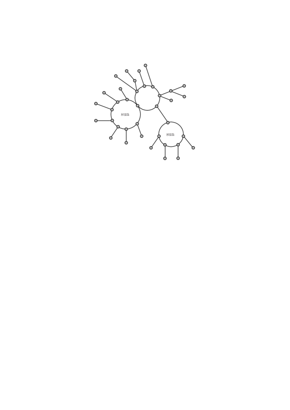
If and are subgraphs of a graph , then the distance between and is defined as , where is the standard distance between vertices and . Let and be cycles of a cactus graph . If and such that , then we say that and are exit vertices of cycles and , respectively. A cycle of is said to be an outer cycle if it has at most one exit vertex. In the case that is unicyclic, then we also declare its cycle to be outer. Hence, if a cactus graph is not a tree, then it contains at least one outer cycle. We say that there is a sun at an outer cycle of a cactus if at all of its vertices, but at the exit vertex, there is exactly one pendant vertex attached. In Fig. 3 a cactus that contains two suns is drawn.
With the above terminology in hands the main result of this section reads as follows.
Theorem 4.1
Let be a connected, bipartite cactus. If contains no sun at an outer cycle, and the exit vertex of every outer -cycle is of degree at least , then .
Proof.
We proceed by induction on the value of the function defined in the previous section. For we have , and . For the inductive hypothesis, let and assume that for every nontrivial graph with , we have , where and are connected, bipartite cactus graphs. If is a tree, then the result follows. Also, if is a cycle, then the statement is true. Thus, we may suppose that contains at least one cycle as a proper subgraph. We denote with , where is an even number, an outer cycle of , and with the exit vertex of .
In the rest of the proof we will consider subgraphs formed from by removing a set of vertices or edges and adding edges in such a way that will hold and such that will fulfil the assumptions of the theorem. Also, throughout the proof, will denote a minimum -domination set of , and an optimal annihilation set in . We are going to construct a -domination set and an annihilation set in that will satisfy . Applying our inductive hypothesis to , we will estimate that and consecutively . In this way the theorem will be proved.
Case 1: All vertices from have degree 2.
Let . Set . Then . Since , both vertices and belong to . Set .Then is a -dominating set of and hence . Since , then and are also both in . Set , Then . It follows that . So .
Case 2: contains a vertex of degree at least .
Since contains some vertices of degree at least , and is an outer cycle, there are trees attached to these vertices. We root each of these trees in the vertex of the tree that lies in . Amongst these trees select a tree such that has the largest height among the trees, where the height of is . Denote the height ot with , and let .
Subcase 2.1: .
Since , there exists a leaf such that . By Lemma 3.3 and our inductive hypothesis, the theorem holds.
Subcase 2.2: .
We consider Cases (a), (b), (c), (d), and (e) which are schematically presented in Fig. 2. All the other cases can be proved with the help of Lemma 3.1 and Lemma 3.2(ii).
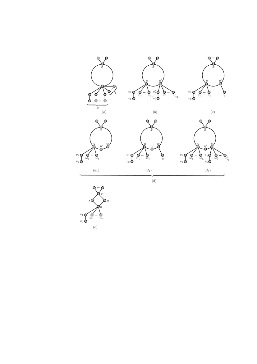
Case (a): In this case, we have a subdivided star , (), attached to the vertex in . By Lemma 3.4 and our inductive hypothesis for , the result holds.
In the following cases we will only consider subdivided stars with and , that is, the subdivided star . Set , where is the vertex of degree , are leaves adjacent to , and is the pendant path of length .
Case (b): In this case there are subdivided stars and with adjacent respective roots and on . Let and . Set
Then . Since , we have . Set further . Since is a -domination set of we get . Let be the neighbor of on different from . (Note that may be .). We now consider four subcases with respect to whether and belong to .
If and , we have . Let . Then , and we have .
If and , we have . Let . Then , and we have .
If and , we have . Let . Then , and we have .
If and , we have . Let . Then , and we have .
Case (c): In this case there exists a subdivided star whose vertex on has a neighbor on with an attended pendant vertex .
If , then let . Then . Setting we have . Independently of whether the neighbors of and in are inside or not, we have . Let . Then , and we have .
Suppose now that and let . If , then we can proceed as in the above case . Suppose next that . Setting we have . Let , and hence . If , then set . Then . If , then set . Then . So we have .
Case (d): In this case we have a subdivided star such that its vertex on , has a neighbor on of degree . We consider thres subcases.
Case (d1): In this subcase has another neighbor such that . If , select . Then . Since =1, we much have . Let . Since is a -dominating set of , we get . Independently of whether the neighbors of and in are inside or not, we have . Let . Then , and we have .
Consider now the case that . Setting we have . Let , and hence . If , then set . Then . If , then set . Then . So we have .
Case (d2): Suppose new that the other neighbor of has a pendant vertex . If , then let . Then . Since =1, we have . Set . Then is a -dominating set of and therefore . If , then we have . Set next . Then , and we have . If , we have . Setting , we have , and we have .
Let now . Setting we have . Let , and hence . If , then set and . If , then set and therefore . So we have .
Case (d3): Suppose now that at the other neighbor of we have another subdivided star . Set and hence . Setting we get . Independently of whether the neighbors of and in are inside or not, we have . Set further , so that , and .
Case (e): Let and let , where is attended with a subdivided star . Setting we have . Since , the vertices and belong to . Let . Then . Set further . Then , and .
Subcase 2.3: .
We need to consider only one case which is shown in Fig. 5, because, as we have already seen in Case 2.2, all the other cases for can be proved with the help of Lemma 3.1.
Assume that , and at least one of its neighbors in , is degree of , denote it with . Denote the child of with . Setting we have . Then , since it is leaf in . Setting we get . Independently of whether the neighbors of in are inside or not, we have . Let . Then , and we have . ∎
5 Concluding remarks
Based on the results of this paper, the following problem is very natural.
Problem 5.1
Characterize the cactus graphs for which Conjecture 1.1 holds true.
Note that the class of cacti in question does not contain bipartite cacti as a subclass since some of the counterexamples from Section 2 are bipartite. More generally, it would be interesting to know the answer to the following:
Problem 5.2
Characterize the graphs for which Conjecture 1.1 holds true.
As we already mentioned, in [9] trees were characterized for which the equality in Conjecture 1.1 holds. Hence we pose:
Problem 5.3
Characterize the cactus graphs for which the equality in Conjecture 1.1 holds. More generally, characterize the graphs with the same property.
Let denote the total domination number of a graph . (For an extensive information on see the book [13].) In [7, 9] a parallel conjecture to Conjecture 1.1 was posed for the total domination number, that is, it was conjectured that
| (2) |
holds for every nontrivial connected graph . This conjecture holds for graphs of minimum degree at least , and has been verified for trees [8] and for cactus graphs and block graphs [2]. The counterexamples to Conjecture 1.1 presented in this paper are far from being counterexamples for (2) since their total domination number is significantly smaller and, after all, the counterexamples to Conjecture 1.1 are cactus graphs for which (2) holds. Hence we are inclined to believe that (2) holds true.
Acknowledgments
Jun Yue was partially supported by the National Natural Science Foundation of China (No. 11626148 and 11701342) and the Natural Science Foundation of Shandong Province (No. ZR2016AQ01). Yongtang Shi was partially supported by the National Natural Science Foundation of China, Natural Science Foundation of Tianjin (No. 17JCQNJC00300), the China-Slovenia bilateral project “Some topics in modern graph theory” (No. 12-6), Open Project Foundation of Intelligent Information Processing Key Laboratory of Shanxi Province (No. CICIP2018005), and the Fundamental Research Funds for the Central Universities, Nankai University (63191516). Sandi Klavžar acknowledges the financial support from the Slovenian Research Agency (research core funding P1-0297 and projects J1-9109, N1-0095, N1-0108).
References
- [1] J. A. Bondy, U. S. R. Murty, Graph Theory, GTM 244, Springer, 2008.
- [2] Cs. Bujtás, M. Jakovac, Relating the total domination number and the annihilation number of cactus graphs and block graphs, Ars Math. Contemp. 16 (2019) 183–202.
- [3] Cs. Bujtás, S. Jaskó, Bounds on the -domination number, Discrete Appl. Math. 242 (2018) 4–15.
- [4] M. Chellali, O. Favaron, A. Hansberg, L. Volkmann, -domination and -independence in graphs: a survey, Graphs Combin. 28 (2012) 1–55.
- [5] Y. Caro, Y. Roditty, A note on the -domination number of a graph, Int. J. Math. Math. Sci. 13 (1990) 205–206.
- [6] P. Dankelmann, F. J. Osaye, Average eccentricity, -packing and -domination in graphs, Discrete Math. 342 (2019) 1261–1274.
- [7] E. DeLaVia, Written on the Wall II (Conjectures of Graffiti.pc), ttp://cms.dt.uh.edu/faculty/delavinae/research/wowII/.
- [8] W.~J.~Desormeaux, T.~W.~Haynes, M.~A.~Henning, Relating the annihilation number and the total domination number of a tree, Discrete Appl. Math. 161 (2013) 349–354.
- [9] W.~J.~Desormeaux, M.~A.~Henning, D.~F.~Rall, A.~Yeo, Relating the annihilation number and the $2$-domination number of a tree, Discrete Math. 319 (2014) 15–23.
- [10] J.~F.~Fink, M.~S.~Jacobson, $n$-domination in graphs, In: Y. Alavi, A. J. Schwenk (Eds.), Graph Theory with Applications to Algorithms and Computer Science, Wiley, New York (1985) 283–300.
- [11] J.~R.~Griggs and D.~J.~Kleitman, Independence and the Havel-Hakimi residue, Discrete Math. 127 (1994) 209–212.
- [12] A.~Hansberg, D.~Meierling, L.~Volkmann, Independence and $k$-domination in graphs, Int. J. Comput. Math. 5 (2011) 905–915.
- [13] M.~A.~Henning, A.~Yeo, Total Domination in Graphs, Springer, New York, 2013.
- [14] M.~Jakovac, Relating the annihilation number and the $2$-domination number of block graphs, Discrete Appl. Math. 260 (2019) 178–187.
- [15] R.~Li, Bounding the graphical parameters by the independent and $k$-domination numbers, Rom. J. Math. Comput. Sci. 8 (2018) 52–57.
- [16] J.~Lyle, S.~Patterson, A note on the annihilation number and $2$-domination number of a tree, J. Comb. Optim. 33 (2017) 968–976.
- [17] R.~D.~Pepper, Binding Independence, Ph.D. thesis, University of Houston, Houston, Texas, 2004.