Self-intersection of the Fallback Stream in Tidal Disruption Events

Abstract

We propose a semi-analytical model for the self-intersection of the fallback stream in tidal disruption events (TDEs). When the initial periapsis is less than about 15 gravitational radii, a large fraction of the shocked gas is unbound in the form of a collision-induced outflow (CIO). This is because large apsidal precession causes the stream to self-intersect near the local escape speed at radius much below the apocenter. The rest of the fallback gas is left in more tightly bound orbits and quickly joins the accretion flow. We propose that the CIO is responsible for reprocessing the hard emission from the accretion flow into the optical band. This picture naturally explains the large photospheric radius (or low blackbody temperature) and typical line widths for optical TDEs. We predict the CIO-reprocessed spectrum in the infrared to be $L_{\nu}\propto\nu^{\sim 0.5}$, shallower than a blackbody. The partial sky coverage of the CIO also provides a unification of the diverse X-ray behaviors of optical TDEs. According to this picture, optical surveys filter out a large fraction of TDEs with low-mass blackholes due to lack of a reprocessing layer, and the volumetric rate of optical TDEs is nearly flat wrt. the blackhole mass in the range $M\lesssim 10^{7}\mathrm{M_{\odot}}$. This filtering also causes the optical TDE rate to be lower than the total rate by a factor of $\sim$10 or more. When the CIO is decelerated by the ambient medium, radio emission at the level of that in ASASSN-14li is produced, but the timescales and peak luminosities can be highly diverse. Finally, our method paves the way for global simulations of the disk formation process by injecting gas at the intersection point according to the prescribed velocity and density profiles.

1 Introduction

Tidal disruption events (TDEs) hold promise for probing the otherwise dormant supermassive blackholes (BHs) at the centers of most galaxies (Rees, 1988). The story starts with simple initial conditions: a star, of certain mass and radius, approaches the BH on a parabolic orbit of certain specific angular momentum. The star can be treated as a point mass until it reaches the tidal radius where the tidal forces exceed the star’s self-gravity. The hydrodynamical disruption phase, despite its complexity, is understood to at least order-unity level, thanks to decades of analytical and numerical studies (e.g., Lacy et al., 1982; Carter & Luminet, 1983; Rees, 1988; Evans & Kochanek, 1989; Laguna et al., 1993; Ayal et al., 2000; Lodato et al., 2009; Stone et al., 2013; Guillochon & Ramirez-Ruiz, 2013; Tejeda et al., 2017; Goicovic et al., 2019; Steinberg et al., 2019; Gafton & Rosswog, 2019). The result is that the post-disruption stellar debris acquires a spread of specific orbital energy, which is roughly given by the gradient of the BH’s gravitational potential across the star at the tidal radius. This means that roughly half of the stellar debris is unbound and the other half is left in highly eccentric bound orbits.

After the disruption phase, the star is tidally stretched into a very long thin stream and the evolution of the stream structure in the transverse and longitudinal directions are decoupled (Kochanek, 1994). Thus, the system enters the free-fall phase where each stream segment follows its own geodesic like a test particle (Coughlin et al., 2016). Then, after passing the apocenters of the highly eccentric orbits, the bound debris falls back towards the BH at a rate given by the distribution of specific energy (Evans & Kochanek, 1989; Phinney, 1989). Due to relativistic apsidal precession, the bound debris, after passing the pericenter, collides violently with the still in-falling stream (see Fig. 1). It has been shown that shocks at the self-intersection point is the main cause of orbital energy dissipation and the subsequent formation of an accretion disk (Rees, 1988; Kochanek, 1994; Hayasaki et al., 2013; Guillochon et al., 2014; Shiokawa et al., 2015; Bonnerot et al., 2016). However, the aftermath of the self-intersection is an extremely complex problem, which depends on the interplay among magnetohydrodynamics, radiation, and general relativity in 3D. No numerical simulations to date have been able to provide a deterministic model for TDEs with realistic star-to-BH mass ratio and high eccentricity (see Stone et al., 2018a, for a review). Many simulations consider either an intermediate-mass BH (e.g. Guillochon et al., 2014; Evans et al., 2015; Shiokawa et al., 2015; Sa̧dowski et al., 2016) or the disruption of a low-eccentricity (initially bound) star (e.g. Bonnerot et al., 2016; Hayasaki et al., 2016). It is unclear how to extrapolate the simulation results to realistic configurations and provide an answer to the following questions: How long does it take for the bound gas to form a circular accretion disk (if at all)? How much radiative energy is released from the system? What fraction of the radiation is emitted in the optical, UV or X-ray bands?

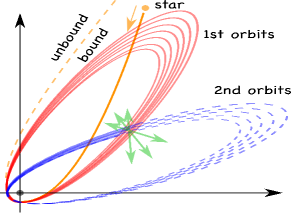
Figure 1: The star was initially in a parabolic orbit (orange curve). After the tidal disruption, the bound materials are in highly eccentric elliptical orbits of different semimajor axes (red curves) but have nearly the same apsidal precession angle per orbit. Materials in their second orbits (blue curves) collide with what is still in the first orbit. The subject of this paper is to study the dynamics of the shocked gas after the collision.

The hope lies in the rapidly growing sample of TDE candidates discovered by recent UV-optical surveys, such as GALEX (Gezari et al., 2008, 2009), SDSS (van Velzen et al., 2011), Pan-STARRS (Gezari et al., 2012; Chornock et al., 2014; Blanchard et al., 2017), PTF (Arcavi et al., 2014; Blagorodnova et al., 2017; Hung et al., 2018), ASAS-SN (Holoien et al., 2014, 2016), and ZTF (van Velzen et al., 2018a), see the open TDE catalog http://tde.space. These events have highly diverse properties in terms of peak optical luminosities, lightcurve shapes, emission line profiles, and optical/X-ray flux ratios. Still, they provide a number of important clues for understanding the dynamics of UV-optical selected TDEs: (1) the photospheric radius of the (thermal) optical emission is typically $\sim$$10^{14}$–$10^{15}\rm\,cm$; (2) the typical widths of H$\alpha$ and/or He II emission lines in the optical band and CIV, NV, SiIV aborption lines in the UV band (e.g. Blagorodnova et al., 2018) are of order $\sim$$10^{4}\rm\,km/s$; (3) the rise/fade timescale is of order $\sim$months; (4) the total energy radiated in the UV-optical band is typically $\lesssim$$10^{51}\rm\,erg$, which is much smaller than the energy budget of the system ($\gtrsim$$10^{53}\rm\,erg$ even for disruption of low-mass stars).

The photospheric radius is much larger than the tidal radius (of order $\sim$$10^{13}\rm\,cm$), and the velocity inferred from line widths is much smaller than the Keplerian/escape velocity near the tidal radius. These properties are inconsistent with the wind-reprocessed emission from a circularized accretion disk near the tidal radius (Strubbe & Quataert, 2009; Miller, 2015). The low radiative efficiency in the optical band is known as the “missing energy” puzzle (Piran et al., 2015; Stone & Metzger, 2016; Lu & Kumar, 2018), whose solution depends on the source of the optical emission. Based on the arguments that the photospheric radius is of the same order as the semimajor axis of the most bound orbit and that the line width roughly agrees with the Keplerian velocity at the same radius, Piran et al. (2015) proposed that the optical emission is powered by the dissipation of orbital energy by stream self-intersection. An alternative phonomelogical model proposed by Metzger & Stone (2016) is that only a small fraction $f_{\rm in}\ll 1$ of the fall-back gas actually accretes onto the BH and the rest $(1-f_{\rm in})$ is blown away by the gravitational energy released from the accreting gas. In this model, if the energy efficiency of accreting gas is $\eta_{\rm acc}=0.1\eta_{\rm acc,-1}$, then the accretion fraction of order $f_{\rm in}\sim 10^{-2}\eta_{\rm acc,-1}^{-1}$. However, these models do not consider the detailed dynamics of the stream self-intersection and disk formation.

In this paper, we consider the stream kinematics in a semi-analytical way and explore the diverse consequences of the stream self-intersection. This approach is similar to Dai et al. (2015) who studied the location and gas velocity at the self-intersection point in a post-Newtonian way (only considering the lowest-order apsidal precession). However, we evolve the system in full general relativity before and after the self-intersection and study the properties of the shocked gas that are unbound, accreting, and plunging. More importantly, instead of assuming inelastic collision as in Dai et al. (2015), we use the realistic equation of state for radiation-dominated gas to model the intersection, motivated by the local simulation of colliding streams by Jiang et al. (2016). Thus, our approach provides a more comprehensive and self-consistent picture of the dynamics and multiwavelength emission from TDEs.

This paper is organized as follows. In §2, we calculate the location of the self-intersection point and the velocities of the two streams before the collision. In §3, we perform hydrodynamical simulation of the collision process. In §4, we consider the fate of the shocked gas after the self-intersection. Implications of TDE dynamics on the multiwavelength observations will be considered in §5. We discuss a number of issues in our modeling in §6. A summary is provided in §7. Unless otherwise specified, we use geometrical units where the gravitational constant and speed of light are $G=c=1$.

2 Self-Intersection of the Fallback Stream

We consider a star of mass $M_{*}=m_{*}\mathrm{M_{\odot}}$ and radius $R_{*}=r_{*}R_{\odot}$ interacting with a BH of mass $M=10^{6}M_{6}\mathrm{M_{\odot}}$. The gravitational radius of the BH is $r_{\rm g}\equiv M$. We take the pericenter of the star’s initial orbit to be $r_{\rm p}=r_{\rm T}/\beta$, where $\beta$ is a free impact parameter describing the depth of penetration and the $r_{\rm T}$ is the Newtonian Roche tidal radius defined as (Hills, 1975)

$${r_{\rm T}\over r_{\rm g}}\equiv{R_{*}\over r_{\rm g}}\left({M\over M_{*}}\right)^{1/3}=46.7\,M_{6}^{-2/3}m_{*}^{-1/3}r_{*}.$$ (1)

The lower limit of the impact parameter $\beta_{\rm min}$ is of order unity, but to obtain its exact value corresponding to marginal disruption, one must take into account relativistic tidal forces and realistic stellar structure/rotation (these will be discussed later in §5.3). After the disruption, the stellar debris attains a spread of specific orbital energy for the stellar debris $\mathcal{E}\in(-\eta_{\rm max}\mathcal{E}_{\rm T},+\eta_{\rm max}\mathcal{E}_{\rm T})$, where we have defined the Newtonian tidal energy

$$\mathcal{E}_{\rm T}\equiv{r_{\rm g}R_{*}\over r_{\rm T}^{2}}=2.13\times 10^{-4}M_{6}^{1/3}m_{*}^{2/3}r_{*}^{-1},$$ (2)

and $\eta_{\rm max}$ is a constant of order unity containing the uncertainties due to stellar structure/rotation and the detailed relativistic disruption process. The Newtonian orbital period of the leading edge ($\eta=\eta_{\rm max}$) is $P_{\rm min}\simeq(41\mathrm{\,d})\,\eta_{\rm max}^{-3/2}M_{6}^{1/2}m_{*}^{-1}r_{*}^{3/2}$.

The bound materials corresponding to $\mathcal{E}<0$ form an elongated thin stream which collides with itself due to apsidal precession (Fig. 1). Since the width of the stream is much smaller than the pericenter radius (e.g., Kochanek, 1994; Coughlin et al., 2016), a given stream segment, characterized by its specific energy $\mathcal{E}=\eta\mathcal{E}_{\rm T}$ and pericenter radius $r_{\rm p}=r_{\rm T}/\beta$ ($\eta\leq\eta_{\rm max}$ and $\beta\gtrsim 1$ are free parameters), moves along a certain geodesic until it collides with the still in-falling gas. Note that we define $\mathcal{E}$ and $r_{\rm p}$ based on Newtonian quantities $\mathcal{E}_{\rm T}$ and $r_{\rm T}$ only for convenience reason, our treatment of the orbital kinematics is fully general relativistic.

In this paper, we consider the simplest case of a non-spinning BH (the effects of BH spin will be discussed in §6). In spherical coordinates for the Schwarzschild spacetime, the initial position of the stream segment is $(t=0,\ r=r_{\rm p},\ \theta=0,\ \phi=0)$ and the proper time of the stream segment starts as $\tau=0$. We align the orbital plane with the equatorial plane of the coordinate system, so $\dot{\theta}\equiv\mathrm{d}\theta/\mathrm{d}\tau=0$. The specific angular momentum of is given by

$$\ell=r_{\rm p}\sqrt{(1+\mathcal{E})^{2}/\mu_{\rm p}-1},\ \mu_{\rm p}\equiv 1-2r_{\rm g}/r_{\rm p},$$ (3)

where $1+\mathcal{E}$ is the total energy including rest mass. Hereafter, the time derivative of any quantity $Q$ with respect to the stream segment’s proper time $\tau$ is denoted by $\dot{Q}$. Measuring the proper time in units of $r_{\rm g}$, we write the geodesic equations

$$\begin{split}\dot{t}&={1+\mathcal{E}\over 1-2r_{\rm g}/r},\ \dot{\phi}=\ell r_{\rm g}/r^{2},\\ \dot{r}^{2}&=(1+\mathcal{E})^{2}-\left(1-{2r_{\rm g}\over r}\right)\left(1+{\ell^{2}\over r^{2}}\right),\\ \ddot{r}&=-{r_{\rm g}^{2}\over r^{2}}+{\ell^{2}r_{\rm g}\over r^{3}}\left(1-{3r_{\rm g}\over r}\right).\end{split}$$ (4)

We use a Leapfrog method to integrate the above geodesic equations with timestep $\delta\tau=r_{\rm g}/30$. Since these two colliding flows have similar specific energies $\eta_{1}\approx\eta_{2}$, the radius for self-intersection $r_{\rm I}$ is approximately given by $\phi(r_{\rm I})=\uppi$.

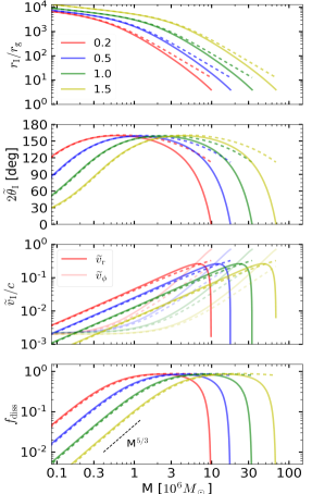
Figure 2: The self-intersection radius, full angle, velocity, and efficiency of orbital energy dissipation as a function of the BH’s mass. The red, blue, green, and yellow curves are for stellar masses of $m_{*}=0.2$, $0.5$, $1.0$, $1.5$ (shown in the legend of the first panel). For all panels, we use the same the impact parameter $\beta=1.0$ ($r_{\rm p}=r_{\rm T}/\beta$) and orbital energy parameter $\eta=1.0$ ($\mathcal{E}=\eta\mathcal{E}_{\rm T}$). The solid curves are from general relativistic (GR) calculations and the dashed curves are the corresponding post-Newtonian results given by Dai et al. (2015). The cut-off of each curve on the high BH mass end is due to direct capture of the star by the BH. In the third panel, we show the radial component $\widetilde{v}_{\rm r}$ in darker curves and transverse component $\widetilde{v}_{\phi}$ in lighter curves, both measured by a local stationary observer at the intersecting point.

For a stationary observer at the intersecting point $r_{\rm I}$, we define $\mu_{\rm I}\equiv 1-2r_{\rm g}/r_{\rm I}$, so the local differential length in the radial direction is $\mathrm{d}\widetilde{r}=\mu_{\rm I}^{-1/2}\mathrm{d}r$ and the local differential time is $\mathrm{d}\widetilde{t}=\mu_{\rm I}^{1/2}\mathrm{d}t=\mu_{\rm I}^{-1/2}(1+\mathcal{E})\mathrm{d}\tau$. In the following, we consider the stream-intersection process in the comoving frame of a local stationary observer at radius $r_{\rm I}$ (LSO frame hereafter), in which any quantity $Q$ is denoted with a tilde $\widetilde{Q}$. Then, the radial and transverse velocities of the colliding streams in the LSO frame are

$$\begin{split}\widetilde{v}_{\rm r}&={\mathrm{d}\widetilde{r}\over\mathrm{d}\widetilde{t}}=\mu_{\rm I}^{-1}{\mathrm{d}r\over\mathrm{d}t}={\dot{r}(r_{\rm I})\over 1+\mathcal{E}},\\ \widetilde{v}_{\rm\phi}&=r_{\rm I}{\mathrm{d}\widetilde{\phi}\over\mathrm{d}\widetilde{t}}={r_{\rm I}\mu_{\rm I}^{1/2}\over 1+\mathcal{E}}\dot{\phi}(r_{\rm I}).\end{split}$$ (5)

The intersecting half angle $\widetilde{\theta}_{\rm I}$ in the LSO frame is given by

$$\mathrm{tan}\,\widetilde{\theta}_{\rm I}={\widetilde{v}_{\rm r}\over\widetilde{v}_{\rm\phi}}={\dot{r}(r_{\rm I})\over\mu_{\rm I}^{1/2}r_{\rm I}\dot{\phi}(r_{\rm I})}.$$ (6)

In Fig. 2, we compare the self-intersection radius, angle, and velocities from our general relativistic calculations with the corresponding lowest-order post-Newtonian results by Dai et al. (2015). We take $\beta=1.0$ and $\eta=1.0$ to be our fiducial parameters. We consider four different stellar masses of $m_{*}=0.2$, $0.5$, $1.0$, $1.5$ and the corresponding zero-age main-sequence stellar radii $r_{*}=0.23$, $0.46$, $0.89$, $1.63$ are taken from Tout et al. (1996) assuming solar metallicity, with errors of a few percent. As expected, we find that, for more massive BHs, the self-intersection occurs closer to the event horizon and the intersecting velocity is larger (the interaction is more violent).

If one assumes that two colliding flows have equal cross-sections and that the collision is completely inelastic, then the radial 4-velocity component $\dot{r}(r_{\rm I})$ gets dissipated and that the transverse 4-velocity component $r_{\rm I}\dot{\phi}(r_{\rm I})$ survives. In this case, we can quantify the efficiency of orbital energy dissipation by defining

$$f_{\rm diss}=\left({\mu_{\rm I}^{1/2}\over\sqrt{1-\widetilde{v}_{\rm r}^{2}-\widetilde{v}_{\rm\phi}^{2}}}-{\mu_{\rm I}^{1/2}\over\sqrt{1-\widetilde{v}_{\rm\phi}^{2}}}\right)(1-\mu_{\rm I}^{1/2})^{-1},$$ (7)

which describes the change in orbital energy divided by the gravitational binding energy at radius $r_{\rm I}$. This (maximum possible) dissipation efficiency is shown in the fourth panel of Fig. 2. In the low BH mass limit $M_{6}\ll 1$, the dissipation of orbital energy by shocks is extremely weak and we asymptotically have $f_{\rm diss}\propto M^{5/3}$ (marked as a black dashed line in the fourth panel), which agrees with the result of Bonnerot et al. (2017a). In those cases, if the circularization is still dominated by stream self-intersection, then the orbit stays highly eccentric for roughly $f_{\rm diss}^{-1}$ rounds and hence the circularization timescale is roughly $f_{\rm diss}^{-1}P_{\rm min}\propto M^{-7/6}$ (since $P_{\rm min}\propto M^{1/2}$). Other mechanisms, e.g. the magneto-rotational instability, may cause angular momentum exchange and drive circularization on a shorter timescale (Chan et al., 2018). As we discuss later in §5.1, TDEs by low-mass BHs typically generates long-lasting eccentric accretion disks which produce long-duration transients. On the other hand, for high-mass BHs $M_{6}\gtrsim 1$, stream intersection causes strong dissipation of orbital energy and hence the orbit may quickly circularize.

In the next section, we show that completely inelastic collision, as assumed by e.g. Dai et al. (2015), is a poor description of the stream dynamics, because the shocked gas is highly optically thick and hence evolves in a nearly adiabatic manner (Jiang et al., 2016).

3 Hydrodynamical Simulations of the Self-Intersecting Shocks

We numerically simulate the stream-stream collision in a special inertia frame described as follows. In the LSO frame, the 4-velocity of the outward-moving stream is $(\widetilde{u}_{\alpha})=(\widetilde{u}_{t},\widetilde{u}_{r},\widetilde{u}_{\theta},\widetilde{u}_{\phi})=\widetilde{\Gamma}(1,\widetilde{v}_{r},0,\widetilde{v}_{\phi})$, where the Lorentz factor is $\widetilde{\Gamma}\equiv(1-\widetilde{v}^{2})^{-1/2}$ and $\widetilde{v}^{2}=\widetilde{v}_{\rm r}^{2}+\widetilde{v}_{\phi}^{2}$. Our simulation box is centered at the self-intersecting point and is moving at velocity $\widetilde{v}_{\phi}$ with respect to the local stationary observer in the $\hat{\phi}$ direction. Thus, in the comoving frame of the simulation box (hereafter the SB frame), the two streams collide head-on with each of them moving at 4-velocity $\bar{u}_{\rm c}=\widetilde{\Gamma}\widetilde{v}_{r}$ and Lorentz factor $\bar{\Gamma}_{\rm c}=(1+\widetilde{\Gamma}^{2}\widetilde{v}_{\rm r}^{2})^{1/2}$, which means

$$\bar{v}_{\rm c}={\widetilde{\Gamma}\widetilde{v}_{r}\over\sqrt{1+\widetilde{\Gamma}^{2}\widetilde{v}_{r}^{2}}}.$$ (8)

Hereafter, any quantity $Q$ in the SB frame is denoted with an overhead bar $\bar{Q}$. In all possible cases, the incoming velocities of the streams in the SB frame are sub-relativistic $\bar{v}_{\rm c}<0.3c$ (see Fig. 2). Due to extreme stretch and adiabatic cooling, the initial streams are dynamically cold with sound speed much less than the bulk velocity $\bar{v}_{\rm c}$. Another property of the initial streams is that the transverse size is much less than the orbital size $\sim$$r_{\rm I}$ (Kochanek, 1994; Coughlin et al., 2016; Bonnerot et al., 2017a). These properties of the problem enable us to use a single non-relativistic hydrodynamic simulation in a flat spacetime to capture the structure of the shocked gas, which is self-similar within a region of size $\ll r_{\rm I}$.

In our simulation, we use an adiabatic ideal gas equation of state $P\propto\rho^{4/3}$. This is motivated by: (1) the high-density shocked gas is radiation pressure dominated, and (2) the shocked gas is highly optically thick before most of the heat is converted back to bulk motion via $PdV$ work (Jiang et al., 2016). The radiative efficiency of the shocked gas is estimated in Appendix B. Since we are concerned with the fate of the majority of the gas with fallback time $\lesssim 10P_{\rm min}$, the adiabatic assumption is a good one. For simplicity, we assume that the two colliding streams have the same cross-section and that there is no offset in the transverse direction. We will discuss the validity of these assumptions and consequences of relaxing them in §6.

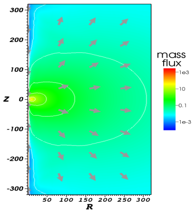
Figure 3: Quasi-steady profiles of the velocity vector field (arrows) and mass flux $\bar{\rho}\bar{v}$ (color image and contours) time t = 0.8, which is 7.5 times the shock-crossing time of the entire simulation domain (or 1200 times the shock-crossing time of the initial streams). At large distances $\gg 10$ from the shocks, velocity vectors are nearly in the radial direction in most directions. This figure is generated with the open source visualization tool VisIt by Childs et al. (2012).

We perform the simulation with the non-relativistic hydrodynamics module of PLUTO (Mignone et al., 2007), solving the mass and momentum conservation equations in 2D cylindrical coordinates ($R,\,z$). The $R$-axis corresponds to the $\hat{\phi}$ direction in the BH rest frame, and the $z$-axis is parallel to the $\hat{r}$ direction in the BH rest frame. The size of our simulation box is $0\leq R\leq 320$ and $-320\leq z\leq 320$. Two identical steady streams are injected in the form of top-hat jets moving in opposite directions at $z=-320$ and $z=320$ in the radius range $0\leq R\leq 1$. The other boundary conditions are as follows: $R=0$ axis-symmetric, $R=320$ outflow, $z=-320$ and $z=320$ outflow (except for the inner cylinder $R\leq 1$ where the streams are injected). The resolution is $\delta R=\delta z=0.125$ ($N_{\rm R}=N_{\rm z}/2=2560$), which means the initial stream is resolved by 8 cells in the transverse direction. The initial streams have mass density 1, pressure $(4/3)^{-1}$, and velocities $\pm 3000$ (all in machine units, since the problem is scale-free in the non-relativistic limit). Since the adiabatic sound speed of the stream is unity, the Mach number is $3000\gg 1$ and hence the streams are effectively cold. The pressure of the ambient medium matches that of the streams. The mass density of the ambient medium is extremely small $10^{-8}$, so the shocked gas expands as if in vacuum. We run the simulation with time step $\delta t\simeq 6\times 10^{-6}$ for a sufficiently long time $t=0.8$ (or 7.5 times the domain crossing time) so that the structure of the shocked gas within a sphere of radius 320 has relaxed to a nearly stable configuration.

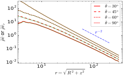
Figure 4: Thick red curves show the radial profiles of the mass flux $\bar{\rho}\bar{v}$ at different polar angles $\bar{\theta}\equiv\mathrm{arctan}(R/z)=30^{\rm o},\ 45^{\rm o},\ 60^{\rm o}$, and $90^{\rm o}$ at t = 0.8. We also over-plot the radial component of the mass flux $\bar{\rho}\bar{v}_{r}$ in thin green curves, which overlap with the red curves. This means that at sufficiently large radii $r>3$, the velocity vectors of the expanding shocked gas are nearly in the radial direction. We can also see that the mass flux is higher near the equatorial plane ($\bar{\theta}\sim 90^{\rm o}$) than that near the poles ($\bar{\theta}\lesssim 30^{\rm o}$). The mass flux profiles asymptotically approach the inverse-square law since $\bar{v}\approx\,$const and $\bar{\rho}\propto r^{-2}$.

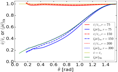
Figure 5: The angular profiles of the velocity and mass flux at three spheres of radii $r=\sqrt{R^{2}+z^{2}}=75$, $150$ and $300$. The polar angle $\bar{\theta}$ is defined as $\bar{\theta}=\mathrm{arctan}(R/z)$. The velocity profiles are normalized by the speed of the incoming stream $\bar{v}_{c}=3000$. At all three radii, the velocity profiles are nearly flat with $\bar{v}\approx\bar{v}_{c}$ at most angles, so we simplify them as an isotropic function $\bar{v}(\bar{\theta})=\bar{v}_{c}$ (yellow curve). The mass flux profiles shown here are simply peak-normalized to illustrate the equatorial concentration near $60^{\rm o}\lesssim\bar{\theta}\leq 90^{\rm o}$. We fit the mass flux profile at $r=300$ with a fourth-order polynomial function (green curve), which is then re-normalized in eq. (10) such that $2\uppi\int_{0}^{\uppi}\bar{\rho}_{\rm n}\sin\bar{\theta}\mathrm{d}\bar{\theta}=1$.

The large-scale structure of the system at $t=0.8$ is shown in Fig. 3. We see that the two streams collide at $z=0$ and the shocked gas expands in a roughly spherical way to radii much larger than the stream width (which equals to unity). In Fig. 4, we show the radial profiles of the mass flux at different polar angles $\bar{\theta}=30^{\rm o},\ 45^{\rm o},\ 60^{\rm o}$, and $90^{\rm o}$. The angular profiles of the velocity and mass flux at three different radii $r=75$, $150$ and $300$ are shown in Fig. 5. We can see that, at large distances from the shocks $r\gtrsim 100$, the velocity profile is very flat but the mass flux is heavily concentrated near the equatorial plane $60^{\rm o}\lesssim\bar{\theta}\leq 90^{\rm o}$. In the following, we simplify the velocity angular profile as isotropic

$$\bar{v}(\bar{\theta})=\bar{v}_{c},$$ (9)

and hence the density angular profile is the same as the mass flux profile. We use a fourth-order polynomial fit to the normalized density angular profile given by

$$\begin{split}\bar{\rho}_{\rm n}&=\sum_{i=0}^{4}q_{i}x^{i},\ q_{0}=1.051\times 10^{-2},\ q_{1}=0.1103,\\ q_{2}&=-0.2017,\ q_{3}=0.2434,\ q_{4}=-0.08436,\end{split}$$ (10)

where $x\equiv\mathrm{min}(\bar{\theta},\,\uppi-\bar{\theta})$ and $2\uppi\int_{0}^{\uppi}\bar{\rho}_{\rm n}\sin\bar{\theta}\mathrm{d}\bar{\theta}=1$.

In the following, we Lorentz transform the velocity and mass flux angular profiles of the shocked gas from the SB frame back to the LSO frame. For a fluid element moving with speed $\bar{v}_{c}$ in an arbitrary ($\bar{\theta},\bar{\phi}$) direction ($\bar{\theta}$ being the polar angle and $\bar{\phi}$ being the azimuthal angle), we write its four-velocity in Cartesian components $(\bar{u}_{\alpha})=\bar{\gamma}(1,\bar{v}_{x},\bar{v}_{y},\bar{v}_{z})$, where $\bar{\gamma}=(1-\bar{v}^{2}_{c})^{-1/2}$, $\bar{v}_{x}=\bar{v}_{c}\sin\bar{\theta}\cos\bar{\phi}$, $\bar{v}_{y}=\bar{v}_{c}\sin\bar{\theta}\sin\bar{\phi}$, and $\bar{v}_{z}=\bar{v}_{c}\cos\bar{\theta}$. The simulation box is moving at velocity $\widetilde{v}_{\phi}$ and the corresponding Lorentz factor is $\widetilde{\Gamma}_{\phi}\equiv(1-\widetilde{v}_{\phi}^{2})^{-1/2}$, so the 4-velocity in the LSO frame is

$$\begin{split}\widetilde{u}_{t}&=\widetilde{\Gamma}_{\phi}\bar{u}_{t}+\widetilde{\Gamma}_{\phi}\widetilde{v}_{\phi}\bar{u}_{x},\ \ \widetilde{u}_{y}=\bar{u}_{y},\\ \widetilde{u}_{x}&=\widetilde{\Gamma}_{\phi}\widetilde{v}_{\phi}\bar{u}_{t}+\widetilde{\Gamma}_{\phi}\bar{u}_{x},\ \ \widetilde{u}_{z}=\bar{u}_{z}.\end{split}$$ (11)

Then, the specific angular momentum and specific energy of this fluid element in the Schwarzschild spacetime are

$$\ell(\bar{\theta},\bar{\phi})=r_{\rm I}\sqrt{\widetilde{u}_{x}^{2}+\widetilde{u}_{y}^{2}},\ 1+\mathcal{E}(\bar{\theta},\bar{\phi})=\mu_{\rm I}^{1/2}\widetilde{u}_{t},$$ (12)

In the next section, we discuss what fraction of the shocked gas is unbound, plunging, or accreting.

4 Fate of the shocked gas after the self-intersection

When the shocked gas expands to a distance much greater than the stream width, the internal pressure becomes low enough that the motion of individual fluid elements is approximately ballistic. If the geodesic reaches infinity or inside the event horizon, we call the fluid element “unbound” or “plunging”, respectively. Those fluid elements with bound but non-plunging geodesics are denoted as “accreting.” The geodesic of a fluid element moving in the ($\bar{\theta},\bar{\phi}$) direction at $r_{\rm I}$ has specific angular momentum $\ell(\bar{\theta},\bar{\phi})$ and specific energy $1+\mathcal{E}(\bar{\theta},\bar{\phi})$, which are given by eq. (12). We note that the marginally bound parabolic orbit for the Schwarzschild spacetime has specific angular momentum $\ell_{\rm mb}=4r_{\rm g}$ and pericenter radius $r_{\rm mb}=4r_{\rm g}$ (Bardeen et al., 1972), so the stream self-intersection radius must always be greater than $4r_{\rm g}$ (see Fig. 2).

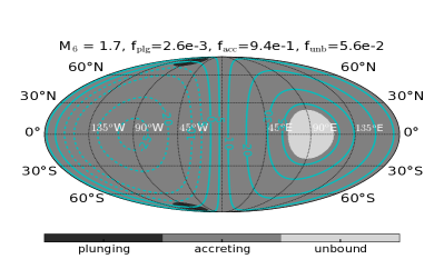
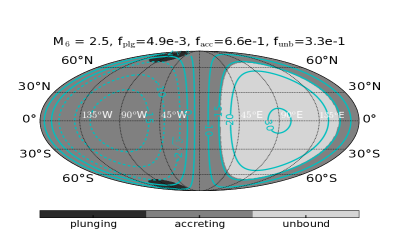
Figure 6: Fate of the shocked gas expanding in different directions ($\bar{\theta}$, $\bar{\phi}$) in the simulation box frame — plunging (black), accreting (dark grey), and unbound (light gray). Here the polar angles $\bar{\theta}=0$ and $\uppi$ correspond to latitudes $90^{\rm o}$ N and $90^{\rm o}$ S, respectively. The azimuthal angles $\bar{\phi}=0$ and $\uppi$ correspond to longitudes $90^{\rm o}$ E and $90^{\rm o}$ W. The mass fraction for the three different fates ($f_{\rm plg}$, $f_{\rm acc}$, $f_{\rm unb}$) are shown in the map title. The upper and lower panels are for BH masses $M_{6}=1.7$ and $2.5$, respectively. We fix the star’s mass $m_{*}=0.5$, impact parameter $\beta=1.0$ ($r_{\rm p}=r_{\rm T}/\beta$) and orbital energy parameter $\eta=1.0$ ($\mathcal{E}=\eta\mathcal{E}_{\rm T}$). The cyan contours are for the specific angular momentum in units of $r_{\rm g}$ projected in the direction of the star’s initial orbital angular momentum. The specific angular momenta of the pre-disruption star are $\ell_{*}=r_{\rm p}\sqrt{1/\mu_{\rm p}-1}=9.0r_{\rm g}$ and $10.2r_{\rm g}$ for BH masses of $M_{6}=1.7$ and $2.5$, respectively. We see that the collision causes significant angular momentum redistribution.

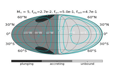
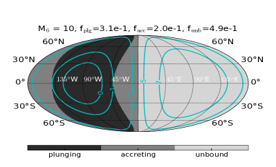
Figure 7: The same as Fig. 6, but for different BH masses $M_{6}=5$ (upper panel) and $10$ (lower panel). The specific angular momenta of the pre-disruption star are $\ell_{*}=12.7r_{\rm g}$ and $16.0r_{\rm g}$ for the two cases of BH masses $M_{6}=5$ and $10$, respectively.

In Fig. 6 and 7, we show the Mollweide projection map of fate in terms of the polar angle $\bar{\theta}$ and azimuthal angle $\bar{\phi}$ in the simulation box frame. Here the polar angle $\bar{\theta}=0$ and $\uppi$ correspond to latitudes $90^{\rm o}$ N and $90^{\rm o}$ S, respectively. The azimuthal angle $\bar{\phi}=0$ and $\uppi$ correspond to longitudes $90^{\rm o}$ E and $90^{\rm o}$ W. The unbound (“unb”), accreting (“acc”), and plunging (“plg”) regions are shown in light grey, dark grey, and black, respectively. For the four cases with different BH masses $M_{6}=1.7,\ 2.5,\ 5,$ and $10$, we fix the star’s mass $m_{*}=0.5$, impact parameter $\beta=1.0$ ($r_{\rm p}=r_{\rm T}/\beta$) and orbital energy parameter $\eta=1.0$ ($\mathcal{E}=\eta\mathcal{E}_{\rm T}$). The cyan contours show the distribution of specific angular momentum (in units of $r_{\rm g}$) projected in the direction of the star’s initial orbital angular momentum. Note that, when determining the fate of a certain fluid element, we take into account its total specific energy and total specific angular momentum. Subsequently, the out-of-plane component of the angular moment will be further damped by shocks within the “accreting” gas. If cooling is efficient, then more gas is expected to plunge into the horizon. We also note that not all fluid elements marked as “plunging” will necessarily fall directly into the horizon. For instance, those moving in the ($\bar{\theta}\sim 0$, $\bar{\phi}\sim\uppi/2$) direction (near the north pole of Fig. 6 and 7) will most likely run into the “accreting” gas. The detailed dynamical evolution of the bound gas is studied in a separate work (Bonnerot & Lu, 2019).

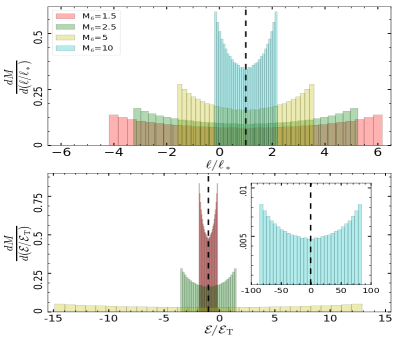
Figure 8: Distributions of specific angular momentum projected along the star’s initial angular momentum (upper panel) and specific orbital energy (lower panel) after the stream self-intersection, for four cases with different BH masses $M_{6}=1.5$, 2.5, 5.0, and 10 (while keeping $\beta=1.0$, $\eta=1.0$, and $m_{*}=0.5$ fixed). Each bin of the histograms is weighted by the gas mass (fraction) within its indicated specific energy or angular momentum range. The overall normalization is such that the integration over all bins is unity. Before the collision, the stream has specific angular momentum $\ell_{0}\approx\ell_{*}=r_{\rm p}\sqrt{1/\mu_{\rm p}-1}$ and orbital energy $-\mathcal{E}_{\rm T}$. Then, the stream collision leads to large spreads of specific angular momentum and orbital energy centered around the initial values. The fluid elements with $\ell<0$ have counter-rotating orbits and those with $\mathcal{E}>0$ are unbound. In the $M_{6}=10$ case (subplot in the lower panel), the fastest moving unbound gas has speed $v_{\rm max}\simeq 0.3$.

In Fig. 8, we show the mass-weighted distributions of specific angular momentum projected along the star’s initial angular momentum and specific orbital energy, for four cases with $M_{6}=1.5$, 2.5, 5, and 10 (while keeping $\beta=1.0$, $\eta=1.0$, and $m_{*}=0.5$ fixed). Before the collision, the stream has specific angular momentum $\ell_{0}\approx\ell_{*}=r_{\rm p}\sqrt{1/\mu_{\rm p}-1}$ and orbital energy $-\mathcal{E}_{\rm T}$. The collision causes a spread of specific angular momentum by $\Delta\ell/\ell_{*}\sim$ a few, and the corresponding spread in the Keplerian circularization radius is about a factor of 10. In some cases (e.g. $M_{6}=1.5$ and 2.5), a large fraction of shocked gas is in counter-rotating orbits ($\ell<0$) and will subsequently collide with the forward-rotating gas ($\ell>0$) at a wide range of radii. The spread in specific orbital energy after the collision is very sensitive to the BH mass, with $\Delta\mathcal{E}/\mathcal{E}_{\rm T}\sim 1$ for $M_{6}=1.5$ but $\Delta\mathcal{E}/\mathcal{E}_{\rm T}\sim 100$ for $M_{6}=10$. For the $M_{6}=1.5$ case, there is no unbound gas. For BH mass $M_{6}\gtrsim 2$, a large fraction of the shocked gas is unbound ($\mathcal{E}>0$). For a highly eccentric Keplerian orbit, the eccentricity is given by $e=\sqrt{1-2|\mathcal{E}|\ell^{2}/r_{\rm g}^{2}}\approx 1-|\mathcal{E}|\ell^{2}/r_{\rm g}^{2}$. We can see that strong shocks due to self-intersection increase the product $|\mathcal{E}|\ell^{2}$ by one order of magnitude or more, and hence the accreting fraction of gas should quickly circularize.

In Fig. 9, we show the mass fractions of the unbound, accreting, and plunging gas as a function of BH mass, for four stellar masses $m_{*}=0.2$, $0.5$, $1.0$, and $1.5$ (while keeping $\beta=1.0$ and $\eta=1.0$ fixed). We find that, above a critical BH mass (to be quantified shortly), the unbound fraction quickly rises from $0\%$ to a maximum of $50\%$. At the same time, the accreting fraction drops from $100\%$ to $50\%$. For higher mass BHs, the plunging fraction quickly rises at the expense of the dropping accreting fraction, while the unbound fraction stays roughly unchanged at $\sim$$50\%$. There is a maximum mass $M_{\rm max}$ above which no accretion is possible, because the entire star plunges into the event horizon.

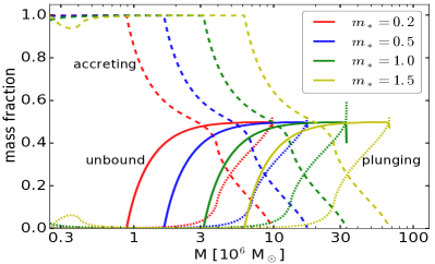
Figure 9: The mass fractions of the unbound (solid), plunging (dashed), and accreting (dotted) gas for different stellar masses $m_{*}=0.2$, $0.5$, $1.0$, and $1.5$. In all cases, we fix the impact parameter $\beta=1.0$ ($r_{\rm p}=r_{\rm T}/\beta$) and orbital energy parameter $\eta=1.0$ ($\mathcal{E}=\eta\mathcal{E}_{\rm T}$). The small bump (or dip) in the plunging (or accreting) fraction for $m_{*}=1.5$ and $M_{6}\sim 0.3$ is because the velocity before the collision has comparable $\hat{r}$ and $\hat{\phi}$ components: $v_{r}\sim v_{\phi}$. See Fig. 20 for the map of fate for this case.

In this paper, we call the unbound fraction of the shocked gas the “collision-induced outflow” (CIO), which has important observational consequences (see the next section). The launching of CIO can be understood in the following Newtonian picture. If the intersection occurs at $r_{\rm p}\ll r_{\rm I}\lesssim r_{\rm a}/3$ ($r_{\rm a}$ being the apocenter radius), then the two streams typically collide at a large angle $2\theta_{\rm I}\gtrsim 90^{\rm o}$ near the local escape speed $|v_{\rm r}\hat{r}+v_{\rm\phi}\hat{\phi}|=\sqrt{v_{\rm r}^{2}+v_{\rm\phi}^{2}}\simeq v_{\rm esc}\simeq\sqrt{2r_{\rm g}/r_{\rm I}}$. The radial velocity component is dissipated by shocks, and then the shocked gas adiabatically expands at speed $\sim$$v_{\rm r}$ in a roughly spherical manner in the SB frame moving at velocity $v_{\rm\phi}\hat{\phi}$. Going back to the LSO frame, we find the fastest moving shocked gas in the ($\bar{\theta}=\uppi/2$, $\bar{\phi}=0$) direction with velocity $(v_{\rm r}+v_{\rm\phi})\hat{\phi}$ and speed $v_{\rm r}+v_{\rm\phi}>\sqrt{v_{\rm r}^{2}+v_{\rm\phi}^{2}}\simeq v_{\rm esc}$. We see that CIO is a generic feature of gas streams colliding near the local escape speed of the intersection point. In Fig. 10, we show the asymptotic kinetic energy and mass-weighted mean speed of the CIO for a number of cases, assuming the total amount of unbound mass to be $f_{\rm unb}m_{*}\mathrm{M_{\odot}}$.

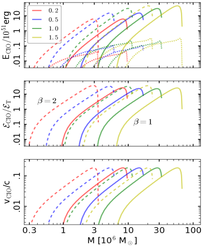
Figure 10: The asymptotic total kinetic energy (upper panel), mean specific energy (middle panel), and mean speed (lower panel) of the CIO for a number of cases with different stellar masses ($m_{*}=0.2$, 0.5, 1.0, and 1.5 as marked in the legend) and impact parameters $\beta=1$ (solid curved) and $2$ (dashed curves). In the upper panel, the dotted lines show the kinetic energy dissipated by collisions within the CIO (see Fig. 11 and 12), which is only a small fraction of the total kinetic energy. We find that, when the unbound fraction is high $f_{\rm unb}\gtrsim 20\%$, the total kinetic energy spans a wide range from $\sim$$10^{50}\rm\,erg$ up to $\sim$$10^{52}\rm\,erg$. When the (mass-weighted) mean specific energy is greater than $\mathcal{E}_{\rm T}$, the CIO is more powerful than the unbound tidal debris. The (mass-weighted) mean speed varies from $\sim$$0.01c$ to $\sim$$0.1c$.

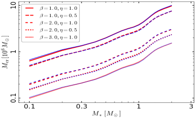
Figure 17: The critical mass above which the unbound fraction exceeds $20\%$, for a number of cases with parameters indicated in the legend. The red curves from numerical calculations almost overlap with the blue curves given by eq. (13).

We define the critical BH mass $M_{\rm cr}$ above which the mass fraction of unbound gas is more than $20\%$, i.e. $f_{\rm unb}(M_{\rm cr})=20\%$. After exploring an extensive grid of parameters (see Fig. 17 in the Appendix), we find

$$M_{\rm cr}\simeq(4.6\times 10^{6}\,\mathrm{M_{\odot}})\,\eta^{0.4}\beta^{-1.7}m_{*}^{-1/2}r_{*}^{3/2}.$$ (13)

This can be translated to a critical pericenter radius

$$r_{\rm p,cr}/r_{\rm g}\simeq 17\,\eta^{-4/15}\beta^{2/15},$$ (14)

below which $f_{\rm unb}\gtrsim 20\%$. If we choose the critical unbound fraction to be $30\%$ (instead of $20\%$), the scalings in the above equations stay the same but the normalization changes to $M_{\rm cr}\simeq 5.3\times 10^{6}\,\mathrm{M_{\odot}}$ (and $r_{\rm p,cr}/r_{\rm g}\simeq 15$). The precise value of the critical unbound fraction is unimportant, because $f_{\rm unb}$ is very sensitive to the BH mass near $M\sim M_{\rm cr}$.

The maximum Schwarzschild BH mass for tidal disruption to occur outside the event horizon can be estimated by requiring $r_{\rm p}=r_{\rm T}/\beta>r_{\rm mb}=4r_{\rm g}$ (since typically $|\mathcal{E}|\ll 1$, see eq. 2),

$$M_{\rm max}\simeq(4.0\times 10^{7}\,\mathrm{M_{\odot}})\,\beta^{-3/2}m_{*}^{-1/2}r_{*}^{3/2}.$$ (15)

Note that the maximum BH mass depends on the minimum impact parameter $\beta_{\rm min}$ at which the relativistic tidal forces exceeds the star’s self-gravity. In the limit $R_{*}\ll 4r_{\rm g}$, the local gravitational-field gradients can described by the relativistic tidal tensor in Fermi normal coordinates. For the Schwarzschild spacetime, the criterion for marginal tidal disruption can be written as

$$r_{\rm p}\approx r_{\rm mb}\approx 5^{1/3}\xi_{*}r_{\rm T},$$ (16)

where the $5^{1/3}$ factor comes from relativistic tidal stretching in the radial direction (Kesden, 2012) and the parameter $\xi_{*}\sim 1$ accounts for the internal structure of the star. We will discuss the choice of $\xi_{*}$ for different stellar masses in §5.3 on TDE demographics. The marginal disruption case occurs when $\ell\approx 4r_{\rm g}$ and $r_{\rm p}\approx 4r_{\rm g}$, which gives the minimum impact parameter $\beta_{\rm min}\approx 5^{-1/3}\xi_{*}^{-1}\simeq 0.6\,\xi_{*}^{-1}$ and the maximum mass for non-spinning BHs associated with TDEs $M_{\rm max,Sch}\approx(8.9\times 10^{7}\mathrm{\mathrm{M_{\odot}}})\,\xi_{*}^{3/2}m_{*}^{-1/2}r_{*}^{3/2}$. We can see that relativistic tidal forces are slightly better at disrupting stars than in the Newtonian approximation. In realistic situations, the precise $\beta_{\rm min}$ (and hence $M_{\rm max}$) will depend on the stellar structure, BH’s spin, star’s spin, and the misalignment between the star’s orbital and the BH’s spin angular momenta, etc. Fortunately, the precise value of $\beta_{\rm min}$ may not be important from the observational point of view, because those TDEs with BH mass close to $M_{\rm max}$ should be quite dim due to their low accreting fraction (most gas is either unbound or plunging, see Fig. 9).

5 Observations

In previous sections, we have described a semi-analytical model for the TDE dynamics, including the fluid properties at the stream self-intersection point and the fate of the shocked gas moving in different directions. In this section, we first discuss the circularization of the fallback stream and the formation of accretion disk in §5.1 and then we consider the observational implications of the unbound gas (when $f_{\rm unb}\neq 0$) in §5.2. TDE demographics will be discussed in §5.3.

5.1 Circularization of the fallback mass

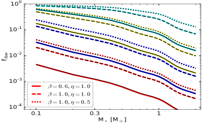
Figure 18: The efficiency of orbital energy dissipation $f_{\rm diss}$ as defined in eq. (7), for $M_{6}=0.03$ (red), 0.1 (blue), 0.3 (yellow) and 1 (cyan curves). For each BH mass, we consider three cases with $(\beta,\eta)=(0.6,1)$ [solid], $(1,1)$ [dashed], and $(1,0.5)$ [dotted curves]. These thick colored curves from numerical calculations overlap with the black thin curves, which are from the analytical expression in eq. (17).

For main-sequence stars disrupted by low-mass BHs ($M_{6}\ll 1$), the stream self-crossing occurs near the apocenter and the shocks only dissipate a small fraction of the orbital energy (see the fourth panel of Fig. 2, and Bonnerot et al., 2016; Chen & Shen, 2018). After exploring an extensive grid of parameters (see Fig. 18 in the Appendix), we find the dissipation efficiency in eq. (7) can be written in the following analytical form for $M_{6}\lesssim 1$

$$f_{\rm diss}=1-{1\over 1+x},\ \mathrm{where}\ x=0.27\,\eta^{-1}\beta^{3}M_{6}^{5/3}m_{*}^{1/3}r_{*}^{-2}.$$ (17)

Note that in the limit $x\ll 1$ ($f_{\rm diss}\approx x$), if the dissipation of orbital energy is only due to stream intersection, then the circularization timescale can be roughly estimated by $f_{\rm diss}^{-1}P_{\rm min}\simeq(152\mathrm{\,d})\,\eta^{-1/2}\beta^{3}M_{6}^{-7/6}m_{*}^{-4/3}r_{*}^{7/2}$. For an average star ($m_{*}\lesssim 1$) disrupted by low-mass BHs $M_{6}\ll 1$, this timescale is much longer than the durations of typical TDEs discovered in recent UV-optical surveys. We also see that tidal disruptions of red giants ($r_{*}\gg 1$) will likely have very long circularization timescales as well, unless they are in deeply penetrating orbits ($\beta\gg 1$).

If MHD turbulence develops rapidly, shear due to magnetic stresses may cause dissipation of orbital energy at a rate (per unit mass) $\dot{\mathcal{E}}_{\rm vis}\sim\alpha\Omega_{\ell}v_{\rm A}^{2}$ (Svirski et al., 2017), where $\alpha\sim 0.1$ is the viscous parameter (Shakura & Sunyaev, 1973), $\Omega_{\ell}(r)=\ell_{*}/r^{2}$ is the local orbital angular frequency, and $v_{\rm A}=\sqrt{B^{2}/4\uppi\rho^{2}}$ is the Alfvén speed. Due to conservation of flux along the stream, the magnetic field strength evolves with radius as $B\propto H(r)^{-2}$, where $H(r)$ is the stream thickness at radius $r$. Right after the disruption, the marginally bound part of the stream moves as $r\propto t^{2/3}$ and the stream length stretches as $r^{2}$, so we obtain the stream density evolution $\rho\propto r^{-2}H(r)^{-2}$ and hence the total viscous heating $\Delta\mathcal{E}_{\rm vis}\sim\dot{\mathcal{E}}_{\rm vis}t\propto r^{3/2}H(r)^{-2}$. The evolution of stream thickness $H(r)$ may be highly complex, depending on tidal forces, self-gravity, magnetic fields, and recombination of hydrogen (Kochanek, 1994; Guillochon et al., 2014; Coughlin et al., 2016). In the limiting case of equilibrium between self-gravity and gas pressure, we have $H\propto\sqrt{P/\rho^{2}}\propto\rho^{-1/6}$ and hence $H(r)\propto r^{1/2}$ (Coughlin et al., 2016), where we have taken a polytropic index of 5/3 which is appropriate before magnetic pressure overwhelms gas pressure or the recombination of hydrogen. In this regime, $\Delta\mathcal{E}_{\rm vis}\propto r^{1/2}$ and most dissipation occurs near the largest radii at which the scaling $H(r)\propto r^{1/2}$ holds. In the other limit where tidal forces dominate over self-gravity, we have $H(r)\propto r$ and $\Delta\mathcal{E}_{\rm vis}\propto r^{-1/2}$, which means that most dissipation occurs near the smallest radii at which the scaling $H(r)\propto r$ holds.

For $\beta\sim\eta\sim 1$, we provide a conservative estimate of the viscous dissipation by assuming the scaling $\Delta\mathcal{E}_{\rm vis}\propto r^{1/2}$ up to the apocenter radius of the most tightly bound orbit $r_{\rm a}$ and obtain

$$\Delta\mathcal{E}_{\rm vis,max}\sim\alpha\,v_{\rm A}^{2}({r_{\rm T}})\sqrt{r_{\rm a}\over r_{\rm T}}.$$ (18)

Since $\alpha\sqrt{r_{\rm a}/r_{\rm T}}\sim\alpha(M/M_{*})^{1/6}\sim 1$, we obtain $\Delta\mathcal{E}_{\rm vis,max}\sim v_{\rm A}^{2}({r_{\rm T}})$, where $v_{\rm A}$ is the Alfvén speed near radius $r_{\rm T}$. The magnetic field may be amplified in the tidal disruption process due to forced differential rotation (Bonnerot et al., 2017b) and the total magnetic energy may be written as $f_{\rm B}GM_{*}^{2}/R_{*}$, where $GM_{*}^{2}/R_{*}$ is the work done by tidal forces and $f_{\rm B}\ll 1$ is the conversion efficiency. Then, we obtain $\Delta\mathcal{E}_{\rm vis,max}\lesssim f_{\rm B}GM_{*}/R_{*}\sim 2\times 10^{-6}f_{\rm B}\ll\mathcal{E}_{\rm T}$, where $\mathcal{E}_{\rm T}$ is the typical orbital energy of the stream (eq. 2). Therefore, the dissipation of orbital energy due to viscous shear is highly inefficient over the orbital timescale.

We also note that dissipation by the nozzle shock operating near the pericenter may also be inefficient, because the ratio between the velocity components perpendicular and inside the star’s orbital plane is of order $H/r\ll 1$. However, this picture may be changed by strong apsidal precession (which causes oblique compression) if the pericenter is close to the horizon $r_{\rm p}\lesssim 10r_{\rm g}$.

Therefore, we conclude that TDEs by low-mass BHs ($M_{6}\ll 1$) have circularization timescale $t_{\rm cir}\gg P_{\rm min}$, which is much longer than the typical duration of the current sample of TDEs discovered by UV-optical surveys. This has important implications on TDE demographics, which will be discussed in §5.3.

In the following, we focus on TDEs by relatively high-mass BHs $M_{6}\gtrsim 1$ where the dissipation of orbital kinetic energy is dominated by stream self-intersection because $f_{\rm diss}\sim 1$. As shown in Fig. 8, the distributions of specific angular momentum and orbital energy are broadened by the collision. The eccentricity $e\simeq 1-|\mathcal{E}|\ell^{2}/r_{\rm g}^{2}$ drops to the level of $1-e\sim 0.1$ due to the increase of the product $|\mathcal{E}|\ell^{2}$ by typically one order of magnitude. Subsequently, the bound gas (and a small fraction of the unbound gas, see §5.2) will collide violently at a wide range of radii between $\sim$$r_{\rm p}$ and $\sim$$r_{\rm I}$ over a timescale $\Omega_{\rm K}^{-1}(r_{\rm I})=c^{-1}\sqrt{r_{\rm I}^{3}/r_{\rm g}}<P_{\rm min}$, where $\Omega_{\rm K}(r_{\rm I})$ is the Keplerian angular frequency for a circular orbit at $r_{\rm I}$. Thus, orbital circularization due to exchange of energy and angular momentum occurs rapidly after the initial stream self-intersection. The detailed dynamics is highly complicated due to the interplay among gas, radiation (providing cooling), and magnetic fields (providing viscosity). This is explored in a separate work (Bonnerot & Lu, 2019).

The most interesting situation is when a significant fraction of the shocked gas becomes unbound in the form of CIO, which occurs for BH masses in the range $M_{\rm cr}<M<M_{\rm max}$. The CIO carries away (positive) energy of $\mathcal{E}\gtrsim\mathcal{E}_{\rm T}$ (see Fig. 8 and 10), and the rest of the shocked gas is left in more tightly bound orbits. The (positive) angular momentum carried away by the CIO is a factor of a few greater than that before the collision, so the remaining bound gas typically have negative angular momentum and hence rotates in the opposite direction of the initial star. Due to subsequent shocks, the counter-rotating gas will quickly settle into circular orbits not at radius $2r_{\rm p}$ but with a radial spread of at least one order of magnitude (even without viscosity).

5.2 Collision-induced Outflow (CIO)

For BH masses in the range $M_{\rm cr}<M<M_{\rm max}$, we find a large fraction of gas is launched in the form of a wide-angle CIO. In the following, we first study the morphology of the CIO (§5.2.1), and then discuss the observational implications of the CIO, including reprocessing the extreme-UV (EUV) or soft X-ray disk emission into the optical band (§5.2.2) and radio emission from the shock driven into the ambient medium (§5.2.3).

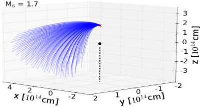
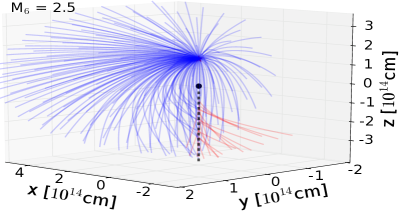
Figure 11: The free-fall trajectories of $\sim$200 fluid elements nearly uniformly distributed within the unbound cone, for two cases with $M_{6}=1.7$ (upper panel), $M_{6}=2.5$ (lower panel). The other parameters $\beta=1.0$, $\eta=1.0$, and $m_{*}=0.5$ are fixed. The integration time (after the stream intersection) for the $M_{6}=1.7$ case is $1.9\,$d and for the $M_{6}=2.5$ case it is $2.2\,$d. For the $M_{6}=2.5$ case, a small fraction of the fluid elements collide with others within the integration time and their free-fall trajectories after the collision (shown in red) are inaccurate. The blue curves show the trajectories without or before collisions. The stream self-intersection point is marked by a red star (at $x=y=0$, $z=r_{\rm I}$) and the BH is marked by a black circle (at $x=y=z=0$).

5.2.1 Morphology of the CIO

We discretize the unbound cone uniformly into $\sim$200 beams and then integrate the geodesics of each beam over longer timescales. We ignore the internal pressure of the CIO based on strong adiabatic cooling during the expansion. The CIO morphologies are shown in Figs. 11 and 12. We see that, within a distance of $\sim$$10^{14}\,$cm, the unbound gas expands into complex morphology and covers a large fraction of the sky viewed from the BH. A small portion of the unbound gas will collide with each other (all along the negative z axis due to BH’s gravitational focusing) and further dissipate their kinetic energy via shocks. For the low BH mass (but $M>M_{\rm cr}$ or $f_{\rm unb}\gtrsim 20\%$) cases, the self-intersection point is far from the event horizon and the gas in the unbound cone is ejected mildly above the local escape speed, so their trajectories are strongly affected by the BH’s gravity (see Fig. 11). For the high BH mass cases, the violent shocks at the intersection point launches unbound gas well above the local escape speed, so their trajectories are almost a straight line (see Fig. 12).

In the Newtonian picture (appropriate at distances $\gg r_{\rm g}$), the peak mass fallback rate of the stream can be estimated

$$\dot{M}_{\rm fb,max}\simeq(3\mathrm{\,\mathrm{M_{\odot}}\,yr^{-1}})\,\eta_{\rm max}^{3/2}M_{6}^{-1/2}m_{*}^{2}r_{*}^{-3/2},$$ (19)

where we have assumed a flat mass distribution over specific energy between $-\eta_{\rm max}\mathcal{E}_{\rm T}$ and $\eta_{\rm max}\mathcal{E}_{\rm T}$ after tidal disruption (e.g. Evans & Kochanek, 1989; Guillochon & Ramirez-Ruiz, 2013). This peak fallback rate lasts for a duration roughly given by the period of the most bound orbit $P_{\rm min}\simeq(41\mathrm{\,d})\,\eta_{\rm max}^{-3/2}M_{6}^{1/2}m_{*}^{-1}r_{*}^{3/2}$. During this time, the time-averaged mass feeding rate to the self-intersecting point is $\dot{M}_{\rm max}\simeq\dot{M}_{\rm fb,max}$ (from both colliding streams). We note that this feeding rate is not constant but modulated by twice the free-fall timescale $2t_{\rm ff}(r_{\rm I})=2\sqrt{r_{\rm I}^{3}/r_{\rm g}}/c=(3.7\mathrm{\,d})(r_{\rm I}/10^{3}r_{\rm g})^{3/2}M_{6}$ in the Newtonian picture, because each segment of length $\sim$$2r_{\rm I}$ will collide with the next segment of the same length. From Figs. 2 and 9, we see that for BH masses $M\gtrsim M_{\rm cr}$, the intersection radius is much below the apocenter radius $r_{\rm I}\ll r_{\rm a}$, so the modulation timescale is much less than the orbital period $2t_{\rm ff}(r_{\rm I})\ll P_{\rm min}$. This discrete mass injection may modulate the optical lightcurve during the early rise segment but not near the peak, because the CIO has highly complex structure with a broad velocity distribution such that the optical flux near the peak is contributed by multiple shells (via photon diffusion, see §5.2.2). On the other hand, if the inner accretion disk is not blocked by the large CIO column for some viewing angles, then the X-ray lightcurve may be strongly affected by the variable mass feeding rate to the accretion disk, provided that the viscous timescale is comparable or shorter than $2t_{\rm ff}(r_{\rm I})$. We also note that hydrodynamic interaction between the fallback stream and the accretion flow may modify the stream’s trajectory and cause the modulation to be non-periodic.

In the next subsection, we show that the CIO generates the optical emission from TDEs. We take an order-of-magnitude approach by assuming that the mass outflowing rate from the self-intersecting point to be steady and the unbound gas expands in a roughly spherical manner at radius $\gg r_{\rm I}$. We ignore the hydrodynamical effects of the wind/radiation from the inner accretion disk. Modeling the full radiative hydrodynamics is left for future works.

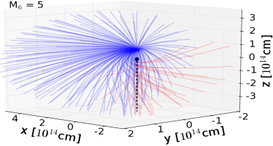
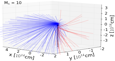
Figure 12: The same as Fig. 11 but for $M_{6}=5$ (upper panel), $M_{6}=10$ (lower panel). The integration time (after the stream intersection) for the $M_{6}=5$ case is $2.2\,$d and for the $M_{6}=10$ case it is $2.5\,$d. Blue curves show the free-fall trajectories without or before collisions and red curves show the (inaccurate) trajectories after the collisions.

5.2.2 Optical emission from TDEs

Optically bright TDEs came as a surprise because the radiation from the inner disk has characteristic temperature

$$\left(\lambda_{\rm Edd}L_{\rm Edd}\over 4\uppi r_{\rm T}^{2}\sigma_{\rm SB}\right)^{1\over 4}\simeq 2.6\times 10^{5}\mathrm{\,K}{\lambda_{\rm Edd}^{1/4}M_{6}^{1/12}m_{*}^{1/6}\over r_{*}^{1/2}},$$ (20)

where $\sigma_{\rm SB}$ is the Stefan-Boltzmann constant and $\lambda_{\rm Edd}$ is the Eddington factor given by the disk bolometric luminosity over the Eddington luminosity $L_{\rm Edd}\simeq 1.5\times 10^{44}\,M_{6}\rm\,erg\,s^{-1}$ (for solar metallicity). TDEs selected as UV-optical transients have photospheric radii $\sim$$10^{14}$–$10^{15}\,\mathrm{cm}\gg r_{\rm T}$ and color temperatures $\sim$a few$\times 10^{4}\,\mathrm{K}$ much less than that given by eq. (20). In the following, we show that the CIO naturally provides the long-sought “reprocessing layer” which absorbs the higher frequency radiation from the inner disk and re-emits at lower frequencies (Loeb & Ulmer, 1997; Guillochon et al., 2014; Metzger & Stone, 2016).

We study the temperature structure of the CIO by assuming a steady-state spherically symmetric structure heated from the bottom at radius $r_{\rm in}\sim\,$a few$\times r_{\rm I}$. We assume the received heating power to be $L_{\rm in}$, which could be in the form of hard emission or wind from the accretion flow.

When the CIO reaches distances $\gg r_{\rm I}$, for a crude estimate, we assume the density and velocity distributions of the outflowing gas to be roughly uniform within a cone of solid angle $\Omega$. Then, the density profile is given by

$$\begin{split}\rho(r)&\simeq{\dot{M}_{\rm max}f_{\rm unb}\over\Omega r^{2}v}\simeq 1.5\times 10^{-12}\mathrm{\,g\,cm^{-3}}{K\over r_{14}^{2}},\\ K&\equiv{2\uppi\over\Omega}{f_{\rm unb}\over 0.5}{\eta_{\rm max}^{3/2}m_{*}^{2}\over M_{6}^{1/2}r_{*}^{3/2}v_{9}},\end{split}$$ (21)

where $f_{\rm unb}$ is the unbound fraction (Fig. 9), $v=10^{9}v_{9}\rm\,cm\,s^{-1}$ is the mass-weighted mean velocity (see the third panel of Fig. 10), and $K$ is the dimensionless “wind constant” which depends on many parameters.

The photon-trapping radius $r_{\rm tr}$, where photon diffusion time equals to the dynamical expansion time, is given by the scattering optical depth $\tau_{\rm s}\simeq\kappa_{\rm s}\rho(r_{\rm tr})r_{\rm tr}\simeq c/v$, i.e.

$$r_{\rm tr}\simeq 1.7\times 10^{14}Kv_{9}\mathrm{\,cm},$$ (22)

where $\kappa_{\rm s}=0.34\rm\,cm^{2}\,g^{-1}$ is the Thomson scattering opacity for solar metallicity. Here we have assumed that the Rosseland-mean opacity roughly equals to the scattering opacity. The scattering photospheric radius $r_{\rm scat}=5.1\times 10^{15}\rm\,cm$ is typically not important in determining the optical appearance of a TDE.

In the radius range $r_{\rm in}<r<r_{\rm tr}$, photons are advected by the expanding wind and the radiation energy density evolves as $U(r)\propto\rho^{4/3}\propto r^{-8/3}$ (Strubbe & Quataert, 2009). Above the radius $r_{\rm tr}$, photons rapidly diffuse away from the local fluid. Since the diffusive flux is given by $F_{\rm diff}\simeq Uc/\tau_{\rm s}\propto r^{-2}$, we have $U(r)\propto r^{-3}$ for $r>r_{\rm tr}$. The normalization for the above scalings for radiation energy density is given by $L_{\rm in}=4\uppi r_{\rm in}^{2}U(r_{\rm in})v$, which means

$$U(r)=8.0\times 10^{5}\mathrm{\,erg\,cm^{-3}}{L_{\rm in,44}r_{\rm in,14}^{2/3}\over r_{14}^{8/3}v_{9}}\mathrm{min}\left[1,\left(r_{\rm tr}\over r\right)^{1/3}\right].$$ (23)

We assume that the radiation is well thermalized near $r_{\rm in}$, so the radiation spectrum is nearly a blackbody up to $r_{\rm tr}$ and the radiation temperature profile is

$$T(r)\simeq 1.0\times 10^{5}\,\mathrm{K}\,{L_{\rm in,44}^{1/4}r_{\rm in,14}^{1/6}\over r_{14}^{2/3}v_{9}^{1/4}}\ \ (\mathrm{for}\ r<r_{\rm tr}).$$ (24)

At larger radii $r>r_{\rm tr}$, the temperature profile depends on whether the majority of photons get thermalized due to a combination of scattering and absorption. In the following, we describe a semi-analytical way of capturing the effect of frequency-dependent thermalization.

At each radius, we define a blackbody temperature $T_{\rm BB}\equiv(U/a)^{1/4}$, which is the temperature the radiation field would have if LTE is achieved. Since the emissivity and absorption opacity are strongly frequency-dependent (due to bound-free edges and lines), it is difficult to achieve an equilibrium between emission and absorption at all frequencies. Instead, we define a rough LTE criterion (see Nakar & Sari, 2010) which is applicable at $r>r_{\rm tr}$,

$$\eta(r)\equiv{U(r)c/4\uppi\over\int\mathrm{d}\nu\,\mathrm{min}\left[B_{\nu}(T_{\rm BB}),j_{\nu}(T_{\rm BB})\,ct_{\rm diff}\right]},$$ (25)

where $B_{\nu}(T_{\rm BB})$ is the Planck function at temperature $T_{\rm BB}$, $j_{\nu}(T_{\rm BB})$ is obtained from Cloudy by assuming the gas is under a thermal radiation bath of temperature $T_{\rm BB}$, and the diffusion time is given by $t_{\rm diff}=\tau_{\rm s}r/c$. Then we dopt a critical value $\eta_{\rm crit}=5/4$ such that the radiation is considered to be in LTE at radii where $\eta(r)<\eta_{\rm crit}$ and non-LTE otherwise. This critical value means that equilibrium between emission and absorption is achieved at about 80% of the frequencies near the peak of the overall spectrum. Thus, the frequency-averaged thermalization radius $r_{\rm th}$ is given by

$$\eta(r_{\rm th})=\eta_{\rm crit}.$$ (26)

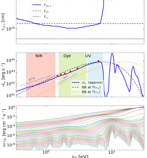
Figure 13: Two possible TDE cases with parameters $(K,v_{9},r_{\rm in,14},L_{\rm in,44})=(1,1,1,1)$ (left panels) and $(3,1,1,3)$ (right panels). Upper Panels: Frequency-dependent thermalization radius given by eq. (28). Note that for the highest frequencies $\gtrsim 20$ eV (left) and $\gtrsim 10$ eV (right), the opacity (due to HeII/HI Ly$\alpha$ and their bound-free transition) is so high that $r_{\rm th,\nu}$ is beyond our radial grid, so our results are unreliable. The trapping radius (eq. 22) and thermalization radius (eq. 26) are shown as dotted and dashed lines. Middle Panels: Spectrum of the escaping photons. We mark the three observational windows: UV ($1700$–$2900\rm\,\AA$), Optical ($3000$–$7000\rm\,\AA$), and NIR ($0.8$–$2.5\rm\,\mu m$). The shallower behavior $\nu L\nu\propto\nu^{1.5}$ (left panel) or $\propto\nu^{1.8}$ (right panel) in the NIR is caused by the increasing $r_{\rm th,\nu}$ towards lower frequencies (due to free-free opacity, see eq. 31), which is a robust prediction of our model. For comparison, we show two blackbody (BB) spectra at temperature $T(r_{\rm th})$ (black dashed) and $T(r_{\rm tr})$ (orange dashed). Data points are the SEDs for two TDEs ASASSN-14li (cyan, left panel, Holoien et al., 2016) and PS1-10jh (red, right panel, Gezari et al., 2012) near peak luminosity. Lower Panels: The (artificially broadened) emissivity at different radii, from $r_{\rm tr}$ (uppermost) to $30r_{\rm tr}$ (lowermost).

Then, the two characteristic radii $r_{\rm tr}$ and $r_{\rm th}$ determine the radial profile of the radiation temperature $T(r)$, which has three power-law segments: $T\propto r^{-2/3}$ ($r_{\rm in}<r<r_{\rm tr}$), $T\propto r^{-3/4}$ ($r_{\rm tr}<r<r_{\rm th}$, assuming $r_{\rm th}<r_{\rm scat}$), and $T=\rm const$ ($r>\mathrm{max}(r_{\rm tr},r_{\rm th})$). Note that in the case where $r_{\rm tr}>r_{\rm th}$, the middle segment does not exist. The mean photon energy the observer sees is given by $2.7k_{\rm B}T[\mathrm{max}(r_{\rm tr},r_{\rm th})]$. With the radiation temperature $T(r)$, energy density $U(r)$, and density $\rho(r)$ at each radius (for a logarithmic radial grid), we use Cloudy to compute the degree of ionization for each chemical species and their energy-level population, under Solar abundance.

We make use of the volumetric emissivity $j_{\nu}(r)$ (for a logarithmic frequency grid) output from Cloudy. At radius $r>r_{\rm tr}$, the energy of photon are still significantly modified by electron scattering. This is because the local intensity distribution is anisotropic with an outwards diffusive flux. This intensity anisotropy means that, at a given radius, an electron scatters more outward-going photons than inward-going ones, and hence photons overall exert a force on this electron. Since the electron is moving outwards at velocity $v$, this force due to photon scattering is doing work to accelerate the electron (of course, this electron is dynamically coupled with a proton such that the actual acceleration is small). The net effect of the photon-electron momentum transfer is that, photons lose a fraction $\sim$$v/(c\tau)$ of energy over each scattering (see Appendix C). Since it takes $\tau^{2}$ scatterings for each photon to escape, the total amount of energy loss is $\sim$$\tau v/c$. We are interested in the region at $r>r_{\rm tr}$ or $\tau<c/v$, so photons lose energy by less than a factor of 2 (and hence overall adiabatic cooling is not important) but this energy shift is important for the transport of line photons by effectively broadening the lines (Pinto & Eastman, 2000; Roth et al., 2016). We take a broadening factor of

$$\sigma=\mathrm{max}(\tau v/c,v/\sqrt{2}c),$$ (27)

and perform a Gaussian kernel smoothing over the Cloudy output of $j_{\nu}(r)$ at each radius.

Now we have all the ingredients to calculate the specific luminosity of the escaping photons from the wind. For each frequency $\nu$, the thermalization radius $r_{\rm th,\nu}$ is given by the equilibrium between emission and absorption, i.e.

$$j_{\nu}(r_{\rm th,\nu})ct_{\rm diff}=B_{\nu}(T_{\rm BB}(r_{\rm th,\nu})),$$ (28)

which is equivalent to the effective absorption optical depth $\tau_{*,\nu}\simeq\sqrt{\tau_{\rm a,\nu}(\tau_{\rm a,\nu}+\tau_{\rm s})}\simeq 1$ (Rybicki & Lightman, 1979). Then, the specific luminosity is roughly given by

$$L_{\nu}\simeq 4\uppi r_{\rm th,\nu}^{3}4\uppi j_{\nu}(r_{\rm th,\nu})\simeq 4\uppi r_{\rm th,\nu}^{2}{4\uppi B_{\nu}(T_{\rm BB}(r_{\rm th,\nu}))\over\tau_{\rm s}(r_{\rm th,\nu})},$$ (29)

where $\tau_{\rm s}(r_{\rm th,\nu})=\kappa_{\rm s}\rho(r_{\rm th,\nu})r_{\rm th,\nu}$. As shown in Fig. 13, our model can reproduce the optical and UV spectral-energy distributions (SEDs) of typical TDE candidates such as ASASSN-14li and PS1-10jh. One robust prediction of our wind reprocessing model is that the SED in the NIR band is softer than that in the optical-UV, typically $L_{\nu}\propto\nu^{\sim 0.5}$. This can be explained as follows.

The absorption opacity in the NIR continuum is dominated by free-free transitions (ignoring the Gaunt factor, Rybicki & Lightman, 1979)

$$\kappa_{\rm low\,\nu}\simeq(1.1\times 10^{17}\mathrm{\,cm^{2}\,g^{-1}})\,\rho T^{-3/2}(h\nu/\mathrm{eV})^{-2},$$ (30)

where the density $\rho$ and temperature $T$ are in units of $\rm g/cm^{3}$ and $\rm K$, respectively. In the limit $\kappa_{\rm low\,\nu}\ll\kappa_{\rm s}$, the effective opacity is given by $\kappa_{\rm*,\nu}\simeq\sqrt{\kappa_{\rm low\,\nu}\kappa_{\rm s}}$ (Rybicki & Lightman, 1979), so the frequency-dependent thermalization radius is given by $\kappa_{\rm*,\nu}\rho r_{\rm th,\nu}\simeq 1$, i.e.,

$$r_{\rm th,\nu}\simeq(3.9\times 10^{14}\mathrm{\,cm})\,(h\nu/\mathrm{eV})^{-1/2}K^{3/4}T_{4.5}^{-3/8},$$ (31)

where $T=10^{4.5}T_{4.5}\rm\,K$ is the electron temperature at the thermalization radius (the final results depends very weakly on $T$). The above equation agrees reasonably well with Fig. 13.

At frequencies with $r_{\rm th,\nu}<r_{\rm tr}$, thermalization occurs below the trapping radius, and the escaping specific luminosity is given by $L_{\nu}=4\uppi r_{\rm tr}^{2}(4\uppi)B_{\nu}(T(r_{\rm tr}))/\tau_{\rm s}(r_{\rm tr})$, which has a blackbody shape at temperature $T(r_{\rm tr})$. However, at frequencies with $r_{\rm th,\nu}>r_{\rm tr}$, thermalization occurs above the trapping radius, and eq. (29) gives

$$\begin{split}\nu L_{\nu}\simeq(2.4\times 10^{41}\mathrm{\,erg\,s^{-1}})\,(h\nu/\mathrm{eV})^{3/2}K^{5/4}T_{4.5}^{-1/8},\end{split}$$ (32)

which applies for at low frequencies (such that $r_{\rm th,\nu}>r_{\rm tr}$)

$$h\nu<(5.2\mathrm{\,eV})\,K^{-1/2}T_{4.5}^{-3/4}v_{9}^{-2}.$$ (33)

This behavior $L_{\nu}\propto\nu^{0.5}$ should be observable in the NIR (see Figs. 4 and 5 of Roth et al., 2016). This effect is analogous to the radio/infrared free-free absorption in the wind of Wolf-Rayet stars (Wright & Barlow, 1975; Crowther, 2007). The weak dependence on the electron temperature $T^{-1/8}$ means that eq. (32) can be used to measure the “wind parameter” $K\propto\dot{M}/v$ for individual TDEs, similar to measuring the mass-loss rate from Wolf-Rayet stars.

5.2.3 Other pieces of information — lines and X-rays

The observed H$\alpha$ and HeII emission lines have complex and sometimes double-peaked or boxy structures (e.g. Arcavi et al., 2014; Holoien et al., 2016, 2018a; Blagorodnova et al., 2018). They have been modeled with the reprocessed emission from an elliptical disk (Liu et al., 2017; Holoien et al., 2018a). However, these elliptical disks may be highly unstable on timescales $\sim$months because each annulus undergoes apsidal precession at a different rate. In our picture, the emission line profiles are mainly controlled by the bulk motion of the line formation region of the CIO (at a few times the trapping radius $r_{\rm tr}$), which can either be blue- or red-shifted depending on the observer’s line of sight. We also note that, if the line formation region has large scattering optical depth, the line profile may be further modified by Comptonization (Roth & Kasen, 2018). The N III and O III emission lines in some TDEs, e.g. AT2018dyb (Leloudas et al., 2019), are probably due to Bowen fluorescence, which requires a large flux of (unseen) EUV photons.

The partial sky coverage of the CIO provides a unification of the diverse X-ray properties of optically selected TDEs. When the line of sight to the inner accretion disk is not blocked by the CIO, the observer should see optical emission as well as the EUV or soft X-ray emission from the inner accretion disk or its wind (Strubbe & Quataert, 2009; Dai et al., 2018; Curd & Narayan, 2019). When the line of sight is only blocked by the region of the CIO with modest optical depth, the observer may see blueshifted absorption lines from high ionization species (e.g. Brown et al., 2018; Blagorodnova et al., 2018). When the line of sight is blocked by the highly optically thick region of CIO, the observer only sees optical emission initially. Then, as the CIO’s mass outflowing rate drops with time, the trapping radius shrinks and hence the EUV and soft X-ray photons from the inner disk suffer less adiabatic loss. As a result, the soft X-ray flux (on the Wien tail) should gradually rise and the spectrum hardens on timescales of $\sim 1\,$yr (Margutti et al., 2017; Gezari et al., 2017; Holoien et al., 2018b).

5.2.4 Radio emission from non-jetted TDEs

In this subsection, we discuss the radio emission from the adiabatic shock driven by the CIO into the circum-nuclear medium (CNM). As shown in Fig. 10, the CIO has kinetic energies from $E_{\rm k}\sim$$10^{50}\rm\,erg$ up to $\sim$$10^{52}\rm\,erg$ and mean speed between $v_{0}\sim$$0.01c$ and $\sim$$0.1c$. In the following, we simplify the complex CIO structure as a thin shell covering a solid angle $\Omega$ within which the density and velocity distributions are uniform. We assume that the ambient medium has a power-law density profile in the radial direction $n=n_{\rm pc}r_{\mathrm{pc}}^{-k}$ ($k<3$), where $r_{\rm pc}=r/\mathrm{pc}$. We also ignore sideway expansion of the shocked region since $\Omega\sim 2\uppi$, so the system is one dimensional.

When the CIO reaches a radius $r$, the total number of shocked electrons from the CNM is given by

$$N(r)=\int^{r}\Omega r^{2}n(r)\mathrm{d}r={\Omega\over 3-k}N_{\rm pc}r_{\rm pc}^{3-k},$$ (34)

where $N_{\rm pc}\equiv n_{\rm pc}\times(1\mathrm{\,pc})^{3}$ is a reference number of electrons. We ignore the acceleration of particles by the reverse shock (driven into the ejecta) because it is much weaker than the forward shock (driven into the CNM). The deceleration radius $r_{\rm dec}$ is given by $E_{\rm k}=(1/2)N(r_{\rm dec})m_{\rm p}v_{0}^{2}$ ($m_{\rm p}$ being proton mass), which means

$$r_{\rm dec,pc}^{3-k}={3-k\over\Omega}{2E_{\rm k}\over N_{\rm pc}m_{\rm p}v_{0}^{2}}.$$ (35)

We smoothly connect the free-expansion phase with the Sedov-Taylor phase by using the following velocity profile

$$v(r)=v_{0}\,\mathrm{min}\left[1,(r/r_{\rm dec})^{(k-3)/2}\right],$$ (36)

and hence the shock reaches radius $r$ at time

$$t(r)={r_{\rm dec}\over v_{0}}\,\mathrm{min}\left[{r\over r_{\rm dec}},{2\over 5-k}\left(r\over r_{\rm dec}\right)^{5-k\over 2}+{3-k\over 5-k}\right].$$ (37)

The electron number density in the shocked region is $4n(r)$ and the mean energy per proton is $(1/2)m_{\rm p}v(r)^{2}$, so the thermal energy density is $2n(r)m_{\rm p}v(r)^{2}$. We assume that a fraction $\epsilon_{\rm B}\ll 1$ of the thermal energy is shared by magnetic fields, so the magnetic field strength is

$$B(r)=\left[16\uppi\,\epsilon_{\rm B}n(r)m_{\rm p}v(r)^{2}\right]^{1/2}.$$ (38)

We assume that electrons share a fraction $\epsilon_{\rm e}\ll 1$ of the thermal energy and that they are accelerated to a power-law momentum distribution with index $p$. We expect particle acceleration from non-relativistic shocks to give $2<p<3$, both theoretically (Bell, 1978; Blandford & Eichler, 1987; Malkov & Drury, 2001; Park et al., 2015; Caprioli & Spitkovsky, 2014) and observationally (Chevalier, 1998; Green, 2014; Zanardo et al., 2014). For fast shocks where the mean energy per electron $\epsilon_{\rm e}m_{\rm p}v^{2}/2\gg m_{\rm e}c^{2}$ ($m_{\rm e}$ being electron mass), the majority of the particle number and kinetic energy are both concentrated near a relativistic minimum momentum $\gg m_{\rm e}c$. For slow shocks where $\epsilon_{\rm e}m_{\rm p}v^{2}/2\lesssim m_{\rm e}c^{2}$, most particles have non-relativistic momenta but the majority of kinetic energy is in mildly relativistic particles with Lorentz factor $\gamma\sim 2$. We are interested in the number density of ultra-relativistic electrons. These two regimes above can be smoothly connected by assuming a power-law Lorentz factor distribution $\mathrm{d}N/\mathrm{d}\gamma\propto\gamma^{-p}$ above the minimum Lorentz factor (Granot et al., 2006; Sironi & Giannios, 2013)

$$\gamma_{\rm m}=\mathrm{max}\left[2,{p-2\over p-1}{\epsilon_{\rm e}m_{\rm p}v(r)^{2}\over 2m_{\rm e}c^{2}}\right].$$ (39)

Then the normalization is given by the total energy of these relativistic electrons being $\epsilon_{\rm e}N(r)m_{\rm p}v(r)^{2}/2$, i.e.,

$$\mathrm{d}N/\mathrm{d}\gamma={\epsilon_{\rm e}m_{\rm p}v(r)^{2}\over 2m_{\rm e}c^{2}}{(p-2)N(r)\over\gamma_{\rm m}^{2}}(\gamma/\gamma_{\rm m})^{-p}.$$ (40)

An electron of Lorentz factor $\gamma\gg 1$ has characteristic synchrotron frequency

$$\nu(\gamma)={3\over 4\uppi}{\gamma^{2}eB\over m_{\rm e}c},$$ (41)

where $e$ is the electron charge. Since the peak specific power is $P_{\nu,\rm max}\simeq e^{3}B/m_{\rm e}c^{2}$, the specific luminosity at frequency $\nu$ in the optically thin regime is given by

$$L_{\nu}\simeq\gamma{\mathrm{d}N\over\mathrm{d}\gamma}{e^{3}B\over m_{\rm e}c^{2}}.$$ (42)

The synchrotron self-absorption frequency $\nu_{\rm a}$ and the corresponding Lorentz factor $\gamma_{\rm a}$ are defined where the optical depth $\alpha_{\nu_{\rm a}}\Delta\ell_{\rm r}\sim 1$ ($\Delta\ell_{\rm r}$ being the radial thickness of the emitting region). The volumetric emissivity at $\nu_{\rm a}$ is given by $j_{\nu_{\rm a}}=\alpha_{\nu_{\rm a}}2kT\nu_{\rm a}^{2}/c^{2}$ (in the Rayleigh-Jeans limit $h\nu_{\rm a}\ll kT$), where $kT\simeq\gamma_{\rm a}m_{\rm e}c^{2}$ is the temperature of electrons responsible for absorption. Assuming $\gamma_{\rm a}>\gamma_{\rm m}$ (which will later be shown to be true for non-relativistic shocks), we can write the specific luminosity as $4\uppi j_{\nu_{\rm a}}\Omega r^{2}\Delta\ell_{\rm r}$, and hence

$$L_{\nu_{\rm a}}=\left.L_{\nu}\right|_{\nu_{\rm a}}\simeq 4\uppi\Omega r^{2}{2kT\nu_{\rm a}^{2}\over c^{2}}.$$ (43)

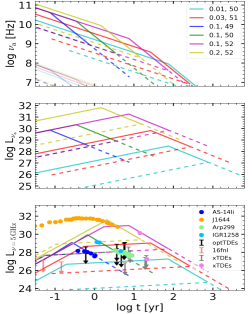
Figure 14: Radio emission from the CIO interacting with the CNM for the case of $k$=1.5, $p$=2.4, $\epsilon_{\rm e}$=0.1, $\epsilon_{\rm B}$=0.01, and $\Omega$=2$\uppi$. The solid and dotted curves are for $n_{\rm pc}$=100 and $3\rm\,cm^{-3}$. Upper panel: The evolution of the synchrotron self-absorption frequency $\nu_{\rm a}$ as a function of time for different cases with initial velocities $v_{0}/c=0.01,\ 0.03,\ 0.1,\ 0.2$ and kinetic energies $\mathrm{log}\,E_{\rm k}\mathrm{/erg}=49,\ 50,\ 51,\ 52$. The fainter curves show $\nu(\gamma_{\rm m})$ which is always much smaller than $\nu_{\rm a}$ (and in some cases always below $10^{6}\,$Hz). Middle panel: The evolution of the peak specific luminosity (in $\rm erg\,s^{-1}\,Hz^{-1}$) with time for the cases indicated in the upper panel. Lower panel: The lightcurve at $5\,$GHz for the cases indicated in the upper panel. We also show the measured fluxes or upper limits at $5\,$GHz for several TDEs in the lower panel, including ASASSN-14li (blue circles, Alexander et al., 2016), Swift J1644+57 (gold circles, Zauderer et al., 2013; Eftekhari et al., 2018), Arp299 (green circles, Mattila et al., 2018), IGR1258 (light blue circles, Irwin et al., 2015; Perlman et al., 2017), iPTF16fnl (red upper limits, Blagorodnova et al., 2017), other optical selected TDEs (black upper limits, van Velzen et al., 2013), X-ray selected TDEs (light blue circles and grey upper limits, Bower et al., 2013).

Combining eqs. (42) and (43), we see that the Lorentz factor $\gamma_{\rm a}$ corresponding to the self-absorption frequency is determined by

$$\left.{\mathrm{d}N\over\mathrm{d}\gamma}\right|_{\gamma_{\rm a}}\simeq{9\Omega r^{2}B\over 2\uppi e}\gamma_{\rm a}^{4},$$ (44)

which gives

$$\gamma_{\rm a}^{4+p}\simeq{2\uppi(p-2)\over 9(3-k)}{e\mathcal{N}_{\rm pc}\over B}{\epsilon_{\rm e}m_{\rm p}v(r)^{2}\over 2m_{\rm e}c^{2}}r_{\rm pc}^{1-k}\gamma_{\rm m}^{p-2},$$ (45)

where we have defined a reference column density $\mathcal{N}_{\rm pc}=n_{\rm pc}\times 1\,$pc. If $\nu(\gamma_{\rm m})\ll\nu_{\rm a}$ and synchrotron/inverse-Compton cooling are negligible, the synchrotron spectrum when the shock is at radius $r$ is given by (Granot & Sari, 2002)

$$L_{\nu}\simeq\begin{cases}L_{\nu_{\rm a}}(\nu/\nu_{\rm a})^{5/2},\ &\mathrm{for}\ \nu(\gamma_{\rm m})<\nu<\nu_{\rm a},\\ L_{\nu_{\rm a}}(\nu/\nu_{\rm a})^{(1-p)/2},\ &\mathrm{for}\ \nu>\nu_{\rm a}.\end{cases}$$ (46)

In Fig. 14, we show the radio emission from CIO colliding with the CNM for a number of cases. We denote the average velocity $v_{0}$ in units of $c$ and the kinetic energy (with unit $\rm erg$) in log-scale. The three cases with $(v_{0},E_{\rm k})=(0.01,50),\ (0.03,51),\ (0.1,52)$ are motivated by the mean velocities and kinetic energies in Fig. 10. The case with $(v_{0},E_{\rm k})=(0.2,52)$ is for comparison with that with $(v_{0},E_{\rm k})=(0.1,52)$, and we see that an outflow with higher velocity generates brighter and earlier-peaked radio emission. The cases with $(v_{0},E_{\rm k})=(0.1,49)$ and (0.1, 50) are motivated by the fact that the CIO velocity profile is non-uniform with a fraction of the mass moving faster than the mean velocity. We find that the faster portion of the ejecta generates bright radio emission at early time. For each combination of $(v_{0},E_{\rm k})$, we take two different CNM density normalizations $n_{\rm pc}=100$ and $3\rm\,cm^{-3}$. As expected, we find that, for higher CNM densities, the radio emission is brighter and peaks earlier.

We also show the data from several TDEs for comparison but do not intend to search for the best-fit parameters for individual cases. The upper limits for iPTF16fnl (Blagorodnova et al., 2017) reported at $15\,$GHz have been scaled by a factor of $(5/15)^{(1-p)/2}$ (assuming $\nu_{\rm a}>5\,$GHz). The upper limits for the X-ray selected TDEs reported at $3\,$GHz by Bower et al. (2013) are not scaled.

Even though we keep the following parameters fixed $k$=1.5, $p$=2.4, $\epsilon_{\rm e}$=0.1, $\epsilon_{\rm B}$=0.01, and $\Omega$=2$\uppi$, the radio luminosity and duration are extremely diverse. Generally, we expect TDEs with CIO to have some radio emission at the level of ASASSN-14li lasting for years up to centuries. We also note that radio emission from the jetted TDE Swift J1644+57 (Bloom et al., 2011; Burrows et al., 2011; Zauderer et al., 2011) is much brighter (and peaks earlier) than that from the CIO, because this source was powered by a relativistic jet pointing towards the observer. For off-axis jetted TDEs, the radio emission due to the CIO may be mistaken as a signature of jets (a possible way of distinguishing between them is to resolve the motion of the radio emitting region by long-baseline interferometry).

Another possible source of wide-angle outflow is the wind expected from super-Eddington accretion in TDEs with BH masses $M\lesssim 10^{7}\mathrm{M_{\odot}}$ (Strubbe & Quataert, 2009; Sa̧dowski et al., 2014; Jiang et al., 2017). In fact, the super-Eddington wind may be more powerful than the CIO, because the energy efficiency of the CIO is only $\sim$$r_{\rm g}/r_{\rm I}\sim 0.001$ to 0.01. Thus, we expect TDEs with strong super-Eddington wind to generate radio emission comparable to or even brighter than that in our $(v_{0},E_{\rm k})=(0.2,52)$ case. Late-time radio observations can potentially test whether super-Eddington accretion flows generate jets or winds. We note that the unbound tidal debris typicall has very small solid angle (Guillochon et al., 2014), so its radio emission (and reprocessing of the high-energy photons from the disk) is much weaker than that of the CIO. It is less likely that the radio emission from ASASSN-14li is caused by the unbound tidal debris (Krolik et al., 2016), unless the star was in a very deeply penetrating $\beta\gg 1$ orbit (Yalinewich et al., 2019).

Finally, we note that the CIO may interact with a pre-existing accretion disk (or the broad line region), if the BH was active before the TDE. If the accretion disk gas is sufficiently dense, the shocks become radiative and bright optical emission like in PS16dtm (Blanchard et al., 2017) may be generated.

5.3 TDE demographics

TDE demographics, in terms of the total TDE rate as a function of BH mass and properties of the disrupted star, has been considered by Stone & Metzger (2016) and Kochanek (2016). In this section, we focus on the rate of optically bright TDEs only, based on the picture that the CIO reprocesses the disk emission from the EUV into the optical band.

We differentiate the TDE rate with three parameters, stellar mass $m_{*}=M_{*}/\mathrm{M_{\odot}}$, impact parameter $\beta$, and BH mass $M$, in the following way

$${\mathrm{d}\dot{n}\over\mathrm{d}m_{*}\,\mathrm{d}\beta\,\mathrm{d}\mathrm{log}M}=\mathcal{R}M_{6}^{\alpha}m_{*}^{-1/12}r_{*}^{1/4}{\mathrm{d}n_{*}\over\mathrm{d}m_{*}}{\mathrm{d}P\over\mathrm{d}\beta}{\mathrm{d}n_{\rm BH}\over\mathrm{d}\mathrm{log}M},$$ (47)

where $\mathcal{R}$ is the normalization rate per BH in units of $\mathrm{yr}^{-1}$, the normalized stellar mass function satisfies $\int(\mathrm{d}n_{*}/\mathrm{d}m_{*})\mathrm{d}m_{*}=1$, the probability distribution of the impact parameter has also been normalized $\int(\mathrm{d}P/\mathrm{d}\beta)\mathrm{d}\beta=1$, and the BH mass function (BHMF) $\mathrm{d}n_{\rm BH}/\mathrm{d}\mathrm{log}M$ has unit $\rm[Mpc^{-3}\,dex^{-1}]$. The factor $m_{*}^{-1/12}r_{*}^{1/4}$ is because stars with a larger tidal radius are slightly preferred roughly by a factor of $r_{\rm T}^{1/4}$ (MacLeod et al., 2012).

The power-law dependence on the BH mass $M^{\alpha}$ depends, in a non-trivial way, on the stellar density and velocity profiles near the center of individual galaxies. The index $\alpha$ is empirically derived by combining the surface brightness profiles of a sample of galaxies with BH masses inferred from galaxy scaling relations (e.g. Magorrian & Tremaine, 1999; Wang & Merritt, 2004; Stone & Metzger, 2016). There is a core-cusp bimodal distribution of central surface brightness profiles of early-type galaxies used for TDE rate calculations (Lauer et al., 2007). The most recent work by Stone & Metzger (2016) gives $\alpha\simeq-0.25$ for samples of only cusp or core galaxies. For comparison, we also show the results for $\alpha\simeq-0.5$ which do not affect our conclusions qualitatively. We caution that the above studies typically assume a spherically symmetric and time-independent galactic potential, nearly isotropic stellar velocity distribution (except for the loss cone), and the refilling of the loss cone by two-body relaxation only. Other factors, such as massive perturbers, aspherical potential, binary BHs, resonant relaxation, may strongly affect the estimated TDE rate (e.g. Vasiliev & Merritt, 2013; Merritt, 2013). Therefore, we leave the normalization factor $\mathcal{R}$ as a free parameter, which roughly means the (per-BH) rate of TDEs for M-dwarf stars disrupted by $\sim$$10^{6}\mathrm{M_{\odot}}$ BHs.

In loss-cone dynamics, the probability distribution for the impact parameter $\mathrm{d}P/\mathrm{d}\beta$ has two regimes. In the “pinhole” regime (far from the BH), the change in stars’ angular momentum per orbit $\Delta\ell$ is much larger than the size of the loss-cone $\ell_{\rm lc}\simeq\sqrt{2r_{\rm g}r_{\rm T}}$, so $\mathrm{d}P/\mathrm{d}\beta$ simply depends on the “area” of the loss cone per unit change in $\beta$, i.e. $\mathrm{d}P/\mathrm{d}\beta\propto\beta^{-2}$. In the “diffusive” regime (near the BH), $\Delta\ell\ll\ell_{\rm lc}$ and hence stars are always disrupted near the boundary of the loss-cone with minimum penetration depth, i.e. $\mathrm{d}P/\mathrm{d}\beta$ is nearly a $\delta$-function. The fraction of TDEs in the pinhole regime $f_{\rm pin}$ depends on the detailed stellar density profile near the BH and has large uncertainty at each BH mass. Following Kochanek (2016), we take

$$f_{\rm pin}\simeq\left(1+M_{7}^{1/2}\right)^{-1},$$ (48)

which is very similar to the fitting result by Stone & Metzger (2016) in the range of BH masses of interest. Then the probability distribution of $\beta$ is given by

$${\mathrm{d}P\over\mathrm{d}\beta}\simeq\begin{cases}f_{\rm pin}\beta^{-2}\beta_{\rm min},\ &\mathrm{for}\ \beta>\beta_{\rm min}\\ (1-f_{\rm pin})\,\delta(\beta-\beta_{\rm min}),\ &\mathrm{for}\ \beta\approx\beta_{\rm min}.\end{cases}$$ (49)

According to eq. (16), the minimum impact parameter is $\beta_{\rm min}\simeq 0.6\,\xi_{*}^{-1}$, which includes relativistic tidal forces for the Schwarzschild spacetime (Kesden, 2012) and $\xi_{*}$ depends on the star’s internal structure. We note that $\xi_{*}$ is not well measured in general relativity even for polytropic stars. Hydrodynamic simulations of disruptions with polytropic or realistic stellar structures in the Newtonian limit ($r_{\rm g}\ll r_{\rm p}$, Guillochon & Ramirez-Ruiz, 2013; Mainetti et al., 2017; Goicovic et al., 2019) show that the star loses about half of the mass when $\xi_{*}\simeq 0.5$ (for polytropic index 4/3) or $\xi_{*}\simeq 1.0$ (for polytropic index 5/3). The former is appropriate for radiative stars with $m_{*}>1.2$ and the latter is good for convective stars with $m_{*}<0.3$ (see a similar treatment by Phinney, 1989). For stars in between $0.3<m_{*}<1.2$, we take a linear interpolation in log$\,m_{*}$ space. Thus,

$$\beta_{\rm min}\simeq\begin{cases}0.6,\ &\mathrm{if}\ m_{*}<0.3,\\ 0.6+\mathrm{log}\,(m_{*}/0.3),\ &\mathrm{if}\ 0.3<m_{*}<1.2,\\ 1.2,\ &\mathrm{if}\ m_{*}>1.2.\end{cases}$$ (50)

We also note that the maximum impact parameter is taken to be infinity, because a star’s orbit can have arbitrarily low angular momentum. The effect of stars being swallowed by the event horizon will be taken into account later when integrating over the BHMF.

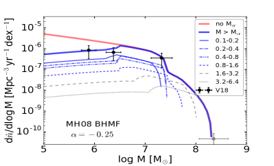
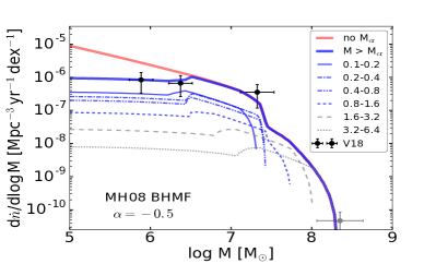
Figure 15: The rate of optically bright TDEs as a function of BH mass is shown in thick blue curve, based on the BHMF of Merloni & Heinz (2008). The upper and lower panels are for $\alpha=-0.25$ and $-0.5$, respectively. The other parameters are fixed: $\mathcal{R}=6\times 10^{-4}\rm\,yr^{-1}$, $\eta=1$, $m_{\rm*,max}=6.4$. The total TDE rate without requiring $M>M_{\rm cr}$ (or the launching of CIO) is shown in red curve. We decompose the TDE rates into six (logarithmic) stellar mass bins as shown in thinner curves: $m_{*}\in(0.1,0.2)$, $(0.2,0.4)$, $(0.4,0.8)$, $(0.8,1.6)$, $(1.6,3.2),(3.2,6.4)$. Including up to the $(1.6,3.2)$ or $(3.2,6.4)$ bin means we are considering a stellar population of relatively young age $\sim$$500\,$Myr or $\sim$$100\,$Myr, respectively. If we take away these two high-mass bins, then the stellar population has age $\sim$$3\,$Gyr. The observationally inferred rates by van Velzen (2018, V18) are shown for comparison. The grey point near $\mathrm{log}M\sim 8.3$ only contains the TDE candidate ASASSN-15lh.

We take the Kroupa initial mass function (IMF, Kroupa, 2001) truncated at $m_{\rm*,max}$ (related to the age of the stellar population)

$${\mathrm{d}n_{*}\over\mathrm{d}m_{*}}=\begin{cases}a_{1}m_{*}^{-1.3},\ &\mathrm{if}\ m_{\rm*,min}<m_{*}<0.5,\\ a_{2}m_{*}^{-2.3},\ &\mathrm{if}\ 0.5<m_{*}<m_{\rm*,max},\\ 0,\ &\mathrm{otherwise}.\end{cases}$$ (51)

The two constants $a_{1}$ and $a_{2}$ are given by the continuity at $m_{*}=0.5$ and normalization $\int(\mathrm{d}n_{*}/\mathrm{d}m_{*})\mathrm{d}m_{*}=1$. We ignore compact stellar remnants since they are fewer in number and are typically swallowed as a whole for $M\gtrsim 2\times 10^{5}\mathrm{M_{\odot}}$. We also ignore red giants, because they have long fallback time $P_{\rm min}\sim 11\mathrm{\,yr}\,M_{7}^{1/2}m_{*}^{-1}(r_{*}/10)^{3/2}$ (and even longer circularization time) and do not have an optically thick layer of gas to reprocess the hard disk emission into the optical band (see §5.2.2). The rate of TDEs contributed by binary stars is lower than that from single stars by a factor of $\sim$$f_{\rm bi}f_{\rm pin}(R_{*}/a)^{3/4}\ll 1$, where $f_{\rm bi}$ is the binary fraction near the galactic center and $a$ is the semimajor axis of the binary orbit. Tidal breakup of the binary has a larger Roche radius $r_{\rm T,b}\simeq(a/R_{*})r_{\rm T}$ and hence occurs at a higher rate than that for single stars by a factor of $\sim$$(a/R_{*})^{1/4}$ (MacLeod et al., 2012). However, stellar disruption is only possible at high impact parameter $\beta\gtrsim a/R_{*}$ in pinhole regime, which means the disruption rate is a factor of $f_{\rm pin}R_{*}/a$ smaller than the tidal breakup rate.

The Kroupa IMF extends down to $m_{*}=0.08$ and then becomes shallower $\mathrm{d}n_{*}/\mathrm{d}m_{*}\propto m_{*}^{0.3}$ for lower mass brown dwarfs. However, TDEs of such low-mass objects likely do not generate much optical emission, the reason being as follows. The mass of the reprocessing CIO can be estimated by $M_{\rm CIO}\sim\rho A\Delta t$ (Lu & Kumar, 2018), where $\rho\simeq(\kappa r_{\rm ph})^{-1}$ is the gas density, $A\simeq L_{\rm opt}/\sigma_{\rm SB}T^{4}\simeq\Omega r_{\rm ph}^{2}$ is the surface area of the optical photosphere, $\kappa$ is the effective absorption opacity, $r_{\rm ph}$ is the photospheric radius, $L_{\rm opt}$ and $T$ are the optical luminosity and blackbody temperature, and $\Delta t$ is the peak duration. Since half of the star’s mass is in unbound tidal debris and only half of the bound mass may be ejected as CIO, we obtain a lower limit for the star’s mass $M_{*}\gtrsim 4M_{\rm CIO}$. Putting in conservative numbers, we obtain

$$M_{*}\gtrsim(0.18\,\mathrm{M_{\odot}})\,{L_{\rm opt,43}^{1/2}v_{9}\over T_{4.5}^{2}\kappa_{-2}}\sqrt{\Omega\over 2\uppi}{\Delta t\over 10\rm\,d}.$$ (52)

Fast transients with $\Delta t\lesssim 10\,$d and $L_{\rm opt}\lesssim 10^{43}\rm\,erg\,s^{-1}$ are increasingly likely to have been missed by current surveys. In the following, we take the conservative minimum stellar mass of $m_{\rm*,min}=0.1$. Larger $m_{\rm*,min}$ will lead to lower rates of optically bright TDEs.

We plug eqs. (49), (51) and a given BH mass function into eq. (47) and calculate the integrated volumetric TDE rate

$$\begin{split}\dot{n}=&\,\mathcal{R}\int_{m_{\rm*,min}}^{m_{\rm*,max}}\mathrm{d}m_{*}\,{r_{*}^{1/4}\over m_{*}^{1/12}}{\mathrm{d}n_{*}\over\mathrm{d}m_{*}}\int_{\beta_{\rm min}}^{\infty}\mathrm{d}\beta\,{\mathrm{d}P\over\mathrm{d}\beta}\\ &\,\int_{M_{\rm cr}}^{M_{\rm max}}\mathrm{d}\mathrm{log}M\,M^{\alpha}{\mathrm{d}n_{\rm BH}\over\mathrm{d}\mathrm{log}M},\end{split}$$ (53)

where the minimum BH mass for CIO launching $M_{\rm cr}$ is given by eq. (13) and the BH mass above which the entire star gets swallowed is given by eq. (15).

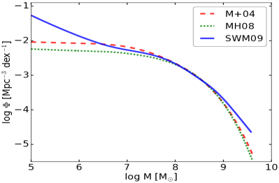
Figure 19: The BHMFs from Marconi et al. (2004, M+04), Merloni & Heinz (2008, MH08), and Shankar et al. (2009, SWM09) used in this paper are shown in red (dashed), green (dotted), and blue (solid) curves.

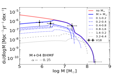
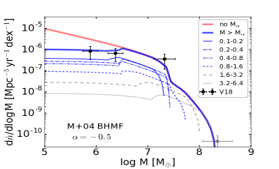
Figure 21: The rate of optically bright TDEs as a function of BH mass, for the BHMF by Marconi et al. (2004). The rate normalization constant is $\mathcal{R}=4\times 10^{-4}\rm\,yr^{-1}$. All other parameters are the same as in Fig. 15.

The BHMF for $M\lesssim 10^{6.5}\mathrm{M_{\odot}}$ is highly uncertain even in the local Universe. Evolutionary models are constructed by inferring BH growth by the “observed” bolometric luminosity function of active galactic nuclei (AGN). Various treatments of bolometric corrections, radiative efficiency of the accretion disks, and AGN duty cycles may give different results. In this paper, we take two different BHMFs for the local Universe by Merloni & Heinz (2008, MH08) and Shankar et al. (2009, SWM09), as shown in Fig. 19 in the Appendix. The main difference between the two lies in the low-mass end: the MH08 mass function is nearly flat while the SWM09 mass function rapidly diverges as $\mathrm{d}n_{\rm BH}/\mathrm{d}\mathrm{log}M\propto M^{-0.6}$. Fig. 15 and Fig. 16 shows the TDE demographics for these two BHMFs, respectively. The BHMF can also be directly calculated by applying correlations between BH mass, bulge luminosity and stellar velocity distribution for galaxies in the local Universe, as done by Marconi et al. (2004). We also tried using their BHMF and found that it gives similar results as the MH08 mass function, as shown in Fig. 21 in the Appendix.

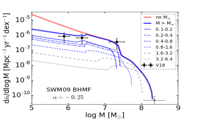
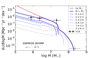
Figure 16: The rate of optically bright TDEs as a function of BH mass, for the BHMF by Shankar et al. (2009). The rate normalization constant is $\mathcal{R}=3\times 10^{-4}\rm\,yr^{-1}$. All other parameters are the same as in Fig. 15.

On the low BH-mass side, the predicted rate of optically bright TDEs is nearly flat with respect to the BH mass. This is because those TDEs with $M<M_{\rm cr}$ have been filtered out due to insufficient amount of CIO being launched. Our results roughly agree with the rate given by van Velzen (2018), which was based on the “V/V_max” method and the BH masses are inferred from galaxy scaling relations with updated stellar velocity dispersion by Wevers et al. (2017). We also show the total TDE rate without requiring $M>M_{\rm cr}$ (red curves), which rises more rapidly towards the low-mass end. This is because TDEs favor smaller BHs by the factor $M^{\alpha}$ (we have taken $\alpha=-0.25$ or $-0.5$) and the BHMF model of Shankar et al. (2009) diverges towards the low-mass end (the MH08 model has a shallower behavior). Unfortunately, the current small-number statistics are not able to discriminate between the two scenarios (shown in blue and red curves) at a significant confidence level.

Thus, our picture predicts that the majority of TDEs by BHs with $M\lesssim 10^{6}\mathrm{M_{\odot}}$ are not optically bright and will hence be missed by current optical transient surveys. The rate of optically bright TDEs is a factor of $\sim$10 or more lower than the total TDE rate. Some of these missing TDEs should be observable by wide field-of-view soft X-ray surveys like eROSITA (Cappelluti et al., 2011) and Einstein Probe (Yuan et al., 2015). Our picture can be tested by comparing the detection rates of TDEs in the X-ray and optical bands, although one should keep in mind that low BH-mass TDEs may have a long circularization timescale due to weak apsidal precession (see §5.1).

On the high BH-mass end, the optically bright TDE rate is strongly suppressed due to stars being swallowed by the event horizon, which has been used as a supportive evidence for the existence of BH event horizon (Lu et al., 2017) and that the observed candidates are actually TDEs (van Velzen, 2018). We note that the grey data point near $\mathrm{log}M\sim 8.3$ only contains the TDE candidate ASASSN-15lh, whose nature is still being debated (Dong et al., 2016; Leloudas et al., 2016; Krühler et al., 2018). In our picture, it can be explained by disruption of a relatively massive star $m_{*}\sim 5$ by a non-spinning BH. Disruption of a Sun-like star by a rapidly spinning BH is also possible, because $\beta_{\rm min}$ can be smaller than $0.6\,\xi_{*}^{-1}$ for a prograde orbit (Kesden, 2012; Leloudas et al., 2016).

Finally, we note that rare post-starburst galaxies are over-represented in the current sample of TDE host galaxies by a factor of $\sim$20 to $\sim$100 (Arcavi et al., 2014; French et al., 2016; Law-Smith et al., 2017; Graur et al., 2018), which may be due to higher stellar density concentration near the galactic centers (e.g. Law-Smith et al., 2017; Stone et al., 2018b). Our method also applies to the group of post-starburst galaxies (with a higher rate normalization constant $\mathcal{R}$), as long as their BHMF is similar to that of the entire galaxy population. An important difference is that the age of the stellar population near the centers of post-starburst galaxies may be significantly younger than that for the other normal galaxies, ranging from 100 Myr to 1 Gyr. This will affect the TDE rate on the high BH-mass end. Another potential difference is that the pinhole fraction $f_{\rm pin}$ may be lower for more cuspy (steeper) stellar density distribution in post-starburst galaxies (Stone et al., 2018b).

6 Discussion

In this section, we discuss a number of issues that require further thoughts in future works.

(1) The stream self-intersection may be delayed due to Lense-Thirring (LT) precession, if the BH’s spin is misaligned with the angular momentum of the stellar orbit (e.g. Kochanek, 1994; Dai et al., 2013; Guillochon & Ramirez-Ruiz, 2015; Hayasaki et al., 2016). For highly eccentric orbits, the angle by which the orbital angular momentum vector precesses over one period is $(\Delta\omega)_{\rm LT}\approx 4\uppi a(r_{\rm g}/2r_{\rm p})^{3/2}\sin i$ (to leading post-Newtonian order), where $a$ is the dimensionless spin of the BH and $i$ is the inclination angle ($i=0$ for spin-orbit alignment). For a given orbit, we express the maximum ratio of the stream width over the distance to the BH as $(H/r)_{\rm max}=f_{\rm H}\beta R_{*}/r_{\rm T}$, where $f_{\rm H}$ describes possible broadening of the stream due to apsidal/LT precession, hydrogen recombination, and magnetic fields. Then, intersection may be avoided for a particular orbit when $(\Delta\omega)_{\rm LT}\gtrsim(H/r)_{\rm max}$, i.e.

$$M_{6}^{4/3}m_{*}^{1/6}r_{*}^{-3/2}\gtrsim 1\,f_{\rm H}\,a^{-1}\beta^{-1/2}.$$ (54)

We can see that TDEs by slowly spinning $a\ll 1$ low-mass $M_{6}\lesssim 1$ BHs are expected to have prompt intersection between the first and second orbits (as shown in Fig. 1). For rapidly spinning high-mass BHs, intersection may be avoided promptly (if $f_{\rm H}\sim 1$) but will eventually occur with a delay. From the point of view of an observer who defines $t=0$ as the moment of stream intersection, the delay itself is not important, since the mass flux of the stream stays unchanged. On the other hand, as long as the intersection occurs between two adjacent orbits (the n-th and the n+1-th, as found by Guillochon & Ramirez-Ruiz, 2015), the intersection radius ($r_{\rm I,LT}$) under LT precession is roughly the same as that without LT precession ($r_{\rm I}$). This is because for most TDEs the apsidal precession angle ($3\uppi r_{\rm g}/r_{\rm p}$) is much larger than the LT precession angle. Thus, the intersection radius $r_{\rm I}$, angle $\widetilde{\theta}_{\rm I}$ and velocity $\widetilde{v}_{\rm I}$ calculated in the Schwarzschild spacetime are similar to those for spinning BHs. Therefore, our model for the hydrodynamical collision process, including redistribution of angular momentum/specific energy and the possibility of launching the CIO, should be largely applicable.

(2) TDE demographics on the high BH-mass end depends on the spin distribution. In the case where the star’s initial angular momentum is parallel to the BH’s spin angular momentum, the pericenter radius of the marginally bound parabolic orbit is $r_{\rm mb}=(1+\sqrt{1-a})^{2}r_{\rm g}$ (Bardeen et al., 1972), where $-1<a<1$ is the spin parameter of the BH ($a<0$ for retrograde orbits). The marginal disruption case corresponds to $r_{\rm p}\approx r_{\rm mb}\approx 5^{1/3}\xi_{*}r_{\rm T}$, which gives the maximum mass for Kerr BHs hosting TDEs

$$M_{\rm max,Kerr}=(8.9\times 10^{7}\mathrm{M_{\odot}})\left(2\over 1+\sqrt{1-a}\right)^{3}{\xi_{*}^{3/2}r_{*}^{3/2}\over m_{*}^{1/2}}.$$ (55)

We can see that the $M_{\rm max,Kerr}$ is strongly affected by the BH spin only when $a\gtrsim 0.5$. The maximum BH mass is also affected by the age of the stellar population ($m_{\rm*,max}$, stellar interior structure $\xi_{*}$, and the number of evolved subgiants). It may be difficult to extract the information on the BH spin distribution from TDE rate on the high BH-mass end. We also note that the critical mass $M_{\rm cr}$ (above which significant amount of CIO is launched) is mainly affected by the spin-independent de Sitter term of the apsidal precession, so the TDE demographics on the low BH-mass end should be insensitive to the BH spin distribution.

(3) We have assumed that the two colliding streams have the same cross-section and that there is no offset in the transverse direction. This is reasonable provided that (i) all processes occurring when the fallback stream passes near the pericenter $r\sim r_{\rm p}$ before the collision are largely reversible and that (ii) the angular stream widths $H/r$ are larger than than the amount of LT precession per orbit. However, there could be many irreversible processes occurring near the pericenter, including: (i) apsidal and LT precession causing the tidal compression to be oblique (instead of perpendicular to the orbital velocity); (ii) mass loss along with the bounce following the tidal compression; (ii) viscosity causing exchange of angular momentum between adjacent shear layers. The general relativistic evolution of the fallback stream over multiple orbits is still an open question, mainly because the extremely large aspect ratio makes it a challenging task for numerical simulations. If these irreversible processes are indeed important and eq. (54) is satisfied, our current model needs two additional parameters: the ratio of the cross-sections of the two colliding streams and the fractional offset in the transverse direction. The hydrodynamics of the stream-stream collision and the subsequent expansion of the shocked gas may be largely modified. This is out of the scope of the current work and should be studied in the future.

(4) The energy radiated in the UV-optical band is typically $\lesssim$$10^{51}\,$erg, which is much smaller than the energy budget of the system, even assuming radiatively inefficient accretion (Piran et al., 2015; Lu & Kumar, 2018). In our picture, this “missing energy” puzzle may be explained in two possible scenarios. The first is that the disk bolometric emission is capped near the Eddington level for an extended amount of time ($\gg P_{\rm min}$) but the CIO reprocesses the disk emission in to the UV-optical band only for a timescale of order $P_{\rm min}$ (then the reprocessed emission moves into the EUV and soft X-ray as the trapping radius shrinks). Since the observed peak UV-optical luminosity is also near the Eddington limit (e.g. Wevers et al., 2017), the efficiency for reprocessing, defined as the observed UV-optical luminosity divided by the intrinsic disk luminosity, is required to be of order unity in this case. The second scenario is that the disk bolometric emission significantly exceeds the Eddington limit (as in the simulations by Jiang et al., 2017), but the reprocessing efficiency is much less than unity. The reason for a low reprocessing efficiency could be that, if $r_{\rm tr}\gg r_{\rm in}$, photons are trapped in the expanding CIO and hence their energy is adiabatically lost in the form of $PdV$ work. However, detailed radiation-hydrodynamic simulations are needed to distinguish between these two scenarios.

7 Summary

We have described a semi-analytical model for the dynamics of TDEs, including the properties of the fallback stream before the self-intersection and the fate of the shocked gas after the intersection. We circumvent the computational challenge faced by previous TDE simulation works by assuming that the post-disruption bound stream follows the geodesics in the Schwarzschild spacetime until the self-intersection. Then we numerically simulate the (non-relativistic) hydrodynamical collision process in a local box at the intersection point. Since the cross-sections of the two colliding streams are much smaller than the size of the orbit and the streams are pressureless (or cold) before the collision, the collision process and the expanding structure of the shocked gas are self-similar. This allows us to explore a wide range of TDE parameter space in terms of the stellar mass, BH mass, and impact parameter. Our method provides a way for global simulations of the disk formation process by injecting gas at the intersection point according to the velocity and density profiles (eqs. 9 and 10) shown in this paper.

The most important observational implication is that a large fraction of the fallback gas can be launched in the form of a collision-induced outflow (CIO) when the BH mass is above a critical value $M_{\rm cr}$ (eq. 13). We propose that the CIO is responsible for reprocessing the accretion disk emission from the EUV or soft X-ray to the optical band. This picture can naturally explain the large photospheric radius of $\sim$$10^{14}$–$10^{15}\,$cm (or low blackbody temperature of a few$\times 10^{4}\,$K), and the typical widths of the H and/or He emission lines. We predict the CIO-reprocessed spectrum in the infrared to be $L_{\nu}\propto\nu^{\sim 0.5}$, shallower than a blackbody. A blackbody fit to the optical SED, as commonly done in the literature, may underestimate the true color temperature. Our picture is different from that of Piran et al. (2015) in that the radiation energy ultimately comes from the accretion flow rather than the stream collision (which is shown to be nearly adiabatic, Jiang et al., 2016). Our model is also different from that of Metzger & Stone (2016) in that we identify the physical origin of the “reprocessing layer” and that this layer is aspherical.

The partial sky coverage of the CIO provides a natural unification of the diverse X-ray behaviors of the optically selected TDEs. Depending on the observer’s line of sight, an optically bright TDE may show strong X-ray emission (when the inner disk is not veiled) or weak/no X-ray emission (when the inner disk is veiled), which agrees with the large range of X-ray to optical peak flux ratios: $\sim$$10^{-4}$ for iPTF16fnl (Blagorodnova et al., 2017), $\sim$$10^{-2}$ for AT2018zr (van Velzen et al., 2018a), and $\sim$1 for ASASSN-14li (Holoien et al., 2016). As the CIO’s mass outflowing rate drops with time, the X-ray fluxes for veiled TDEs may gradually rise with time, as observed in ASASSN-15oi and -15lh (Margutti et al., 2017; Gezari et al., 2017; Holoien et al., 2018b). Our picture is different from those of Dai et al. (2018) and Curd & Narayan (2019) which describe that the X-ray to optical flux ratio is controlled by the observer’s viewing angle with respect to rotational axis of the accretion disk (instead of the CIO’s outflowing direction).

In cases where the CIO is launched (BH mass $M>M_{\rm cr}$), the rest of the fallback gas is left in more tightly bound orbits with higher (sometimes negative) specific angular momentum than the original star, and hence the circularization process is expected to occur on timescale of order $\sim$$P_{\rm min}$ after the onset of intersection. If this is confirmed by future simulations, then it explains the rise/fade timescale ($\sim$months) of optically bright TDEs. We note that the circularization radius of the accreting gas may be different from $2r_{\rm p}$ (as generally assumed in the literature, e.g. Rees, 1988; Strubbe & Quataert, 2009; Shen & Matzner, 2014). Another unexpected prediction is that, in some cases, the accretion disk rotates in the opposite direction as that of the initial star.

The total kinetic energy of the CIO spans a wide range from $\sim$$10^{50}$ up to a few$\times 10^{52}\,$erg (in rare cases). The mass-weighted mean speed varies from $\sim$$0.01c$ to $\sim$$0.1c$. The shocks driven into the ambient medium by this outflow can produce radio emission with highly diverse timescales and peak luminosities, depending on the density profile of the ambient medium, CIO’s velocity and energy, and microphysics of particle acceleration/magnetic field amplification by the shocks. The radio emission from ASASSN-14li and a few other TDE candidates may be from the afterglow of the CIO (instead of the unbound tidal debris, which typically has a much narrower solid angle).

We also find that the volumetric rate of optically bright TDEs is nearly flat with respect to the BH mass in the range $M\lesssim 10^{7}\mathrm{M_{\odot}}$. This is because TDEs with $M<M_{\rm cr}$ have been filtered out due to lack of significant amount of CIO. Our results roughly agree with the BH mass function of optically selected TDEs obtained by van Velzen (2018). This filtering leads to an optical TDE rate that is a factor of $\sim$10 or more lower than the total TDE rate (without requiring $M<M_{\rm cr}$). For TDEs by BHs with $M<M_{\rm cr}$, the stream self-intersection becomes less and less efficient at dissipating the orbital energy and other mechanisms such as MHD turbulence may be responsible for driving the formation of a circular disk. The circularization timescale of these TDEs may be much longer than $P_{\rm min}$. Some of them should be observable by wide field-of-view X-ray surveys like eROSITA (Cappelluti et al., 2011) and Einstein Probe (Yuan et al., 2015). Our model can be tested by comparing the rates of TDEs in the X-ray and optical bands.

8 acknowledgments

We are grateful for the discussions with with Eliot Quataert and Tony Piro on the radiative transfer in a reprocessing wind, with Brian Metzger and Dan Kasen on the absorption opacity, and with Sterl Phinney on the effects of stellar interior structure. We also thank Phil Hopkins, Bing Zhang, Shri Kulkarni, Brad Cenko, Sjoert van Velzen, and Jim Fuller for useful conversations. We are indebted to Brian Metzger and Pawan Kumar for reading an earlier version of the manuscript and providing valuable comments. We acknowledge the Texas Advanced Computing Center (TACC) at The University of Texas at Austin for providing HPC resources that have contributed to the research results reported within this paper. This research benefited from interactions at the ZTF Theory Network Meeting, funded by the Gordon and Betty Moore Foundation through Grant GBMF5076 and by the National Science Foundation under Grant No. NSF PHY-1748958. WL was supported by the David and Ellen Lee Fellowship at Caltech.

Appendix A Supplemental Figures

In the Appendix, we provide a number of figures to support the main content. Their descriptions are in the captions.

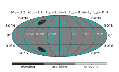
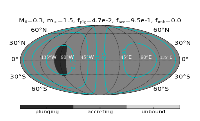
Figure 20: The map of fate for the shocked gas expanding in different directions for two cases with stellar masses $m_{*}=1.0$ (upper panel) and $1.5$ (lower panel). The other conditions are the same: BH mass $M_{6}=0.3$, impact parameter $\beta=1.0$, and orbital energy parameter $\eta=1.0$. In these two cases, the plunging regions are far from the poles ($\bar{\theta}\sim 0$ or $\uppi$), because the velocity before the collision has comparable $\hat{r}$ and $\hat{\phi}$ components: $\widetilde{v}_{\phi}\sim\widetilde{v}_{r}$ (see the third panel of Fig. 2). The specific angular momenta of the pre-disruption star are $\ell_{0}\approx 6.5r_{\rm g}$ (upper panel) and $8.0r_{\rm g}$ (lower panel).

Appendix B Low Radiative Efficiency of Self-intersection Shocks

We justify the usage of adiabatic equation of state for our hydrodynamic simulation in §3. At the collision point, the Thomson scattering optical depth of the stream in the transverse direction is given by $\tau_{\rm st}\simeq 2\kappa_{\rm s}\rho H$, where $H$ is the radius of the stream (assuming cylindrical shape), $\rho$ is the gas density, and $\kappa_{\rm s}=0.34\rm\,cm^{2}\,s^{-1}$ is the scattering opacity. The mass flowing rate of the stream is $\dot{M}_{\rm fb}\simeq\uppi H^{2}\rho v$, and hence

$$\tau_{\rm st}\simeq{2\kappa_{\rm s}\dot{M}\over\uppi Hv}\sim 6\times 10^{3}{\dot{M}_{\rm fb}\over\rm\mathrm{M_{\odot}}\,yr^{-1}}{10R_{\odot}\over H}{0.1c\over v},$$ (56)

where we have used conservative values for the flow velocity $v$, transverse radius $H$, and mass flowing rate (see eq. 19). After the collision, the pressure of the shocked gas is dominated by radiation, and adiabatic expansion converts internal energy back into (roughly spherical) bulk motion over a radius of $r$$\,\sim\,$a few$\times H$. Beyond this radius, the gas expands with nearly constant velocity $v$ and the density drops with radius as $\rho\propto r^{-2}$ (see Fig. 4). Radiation is advected by the expanding shocked gas until the photon trapping radius $r_{\rm tr}\simeq\kappa_{\rm s}\dot{M}/(4\uppi c)$. The radiative efficiency, i.e. the ratio between the emergent luminosity and the total kinetic power, is roughly given by

$$\left(H\over r_{\rm tr}\right)^{2/3}\sim 5\times 10^{-2}\left(\dot{M}_{\rm fb}\over\rm\mathrm{M_{\odot}}\,yr^{-1}\right)^{-{2/3}}\left(H\over 10R_{\odot}\right)^{2/3}.$$ (57)

We see that the stream self-intersection is radiatively inefficient.

Appendix C Photon Down-scattering in Diffusion Region

Consider photons diffusing through a scattering slab in the $\hat{\boldsymbol{x}}$ direction. For a general form of angular dependence for the intensity

$$I(x,\mu)=\sum_{n=0}^{\infty}I_{n}(x)P_{n}(\mu),\ \ \mu\equiv\cos\theta\in[-1,1],$$ (58)

where $I=\int\mathrm{d}\nu I_{\nu}$, $P_{n}(\mu)$ are the Legendre polynomials (only the first three terms are important here) $P_{0}=1$, $P_{1}=\mu$, $P_{2}=(3\mu^{2}-1)/2$, and the orthonormality gives $\int P_{m}P_{n}\mathrm{d}\mu=2\delta_{mn}/(2n+1)$ ($\delta_{mn}$ being the Kronecker delta). The energy density, flux, and pressure of the radiation field are given by the different moments of intensity $U=(2\uppi/c)\int I(\mu)\mathrm{d}\mu=4\uppi I_{0}/c$, $F=2\uppi\int I(\mu)\mu\mathrm{d}\mu=4\uppi I_{1}/3$, and $P=(2\uppi/c)\int I(\mu)\mu^{2}\mathrm{d}\mu=(4\uppi/3c)(2I_{2}/5+I_{0})$. Now take an electron moving at velocity $\beta c$ and Lorentz factor $\gamma$ in the $\hat{\boldsymbol{x}}$ direction. We Lorentz transform the radiation field from the lab frame to the comoving frame of the electron, where quantities are denoted with a prime (^′). In the comoving frame, the electron gains momentum $\Delta p^{\prime}$ over time $\Delta t^{\prime}$ due to scattering

$$\begin{split}{\Delta p^{\prime}\over\Delta t^{\prime}}&={2\uppi\sigma_{\rm T}\over c}\int\mathrm{d}\mu^{\prime}\mu^{\prime}\int\mathrm{d}\nu^{\prime}I^{\prime}_{\nu^{\prime}}(\mu^{\prime})\\ &={2\uppi\gamma^{2}\sigma_{\rm T}\over c}\int\mathrm{d}\mu I(\mu)(\mu-\beta)(1-\beta\mu),\end{split}$$ (59)

where $\sigma_{\rm T}$ is the Thomson cross-section. Making use of the orthonormality relations, the integral above can be expressed in terms of $I_{0}$, $I_{1}$, and $I_{2}$ and hence $U$, $F$, and $P$. Going back to the lab frame, the electron gains energy at a rate given by

$${\Delta E\over\Delta t}=\beta c{\Delta p^{\prime}\over\Delta t^{\prime}}=\gamma^{2}\beta\sigma_{\rm T}c\left[(1+\beta^{2}){F\over c}-\beta(U+P)\right],$$ (60)

which is at the expense of radiation energy. Therefore, the fractional energy loss of a photon under each scattering (over a timescale $\lambda_{\rm mfp}/c$) is given by

$${\delta\nu\over\nu}=-{\Delta E\over\Delta t}{\lambda_{\rm mfp}\over c}{n_{\rm e}\over U}=-\gamma^{2}\beta\left[(1+\beta^{2}){F\over Uc}-\beta\left(1+{P\over U}\right)\right],$$ (61)

where the mean free path is $\lambda_{\rm mfp}=(n_{\rm e}\sigma_{\rm T})^{-1}$. In the limit of isotropic radiation field $F=0$ and $P/U=1/3$, the result $\delta\nu/\nu=4\gamma^{2}\beta^{2}/3$ agrees with Rybicki & Lightman (1979, eq. 7.16a). In the diffusion region of the (non-relativistic) CIO, $r_{\rm tr}<r<r_{\rm scat}$, the diffusive flux is given by $F\simeq Uc/\tau_{\rm s}\gg\beta$ ($\tau_{\rm s}$ being the scattering optical depth), so the fractional energy shift per scattering is

$$\delta\nu/\nu\simeq\beta F/(Uc)=\beta/\tau.$$ (62)

Since a typical photon undergoes $\sim$$\tau^{2}$ scatterings before escaping, the cumulative fractional energy shift is $\tau^{2}\delta\nu/\nu\sim\beta\tau$. This justifies eq. (27).

References

- Alexander et al. (2016) Alexander K. D., Berger E., Guillochon J., Zauderer B. A., Williams P. K. G., 2016, ApJL, 819, L25
- Arcavi et al. (2014) Arcavi I., et al., 2014, ApJ, 793, 38
- Ayal et al. (2000) Ayal S., Livio M., Piran T., 2000, ApJ, 545, 772
- Bardeen et al. (1972) Bardeen J. M., Press W. H., Teukolsky S. A., 1972, ApJ, 178, 347
- Begelman (1979) Begelman M. C., 1979, MNRAS, 187, 237
- Bell (1978) Bell A. R., 1978, MNRAS, 182, 147
- Blagorodnova et al. (2017) Blagorodnova N., et al., 2017, ApJ, 844, 46
- Blagorodnova et al. (2018) Blagorodnova N., et al., 2018, preprint, (arXiv:1809.07446)
- Blanchard et al. (2017) Blanchard P. K., et al., 2017, ApJ, 843, 106
- Blandford & Begelman (2004) Blandford R. D., Begelman M. C., 2004, MNRAS, 349, 68
- Blandford & Eichler (1987) Blandford R., Eichler D., 1987, Physics Reports, 154, 1
- Bloom et al. (2011) Bloom J. S., et al., 2011, Science, 333, 203
- Bonnerot & Lu (2019) Bonnerot C., Lu W., 2019, arXiv e-prints, p. arXiv:1906.05865
- Bonnerot et al. (2016) Bonnerot C., Rossi E. M., Lodato G., Price D. J., 2016, MNRAS, 455, 2253
- Bonnerot et al. (2017a) Bonnerot C., Rossi E. M., Lodato G., 2017a, MNRAS, 464, 2816
- Bonnerot et al. (2017b) Bonnerot C., Price D. J., Lodato G., Rossi E. M., 2017b, MNRAS, 469, 4879
- Bower et al. (2013) Bower G. C., Metzger B. D., Cenko S. B., Silverman J. M., Bloom J. S., 2013, ApJ, 763, 84
- Brown et al. (2018) Brown J. S., et al., 2018, MNRAS, 473, 1130
- Burrows et al. (2011) Burrows D. N., et al., 2011, Nature, 476, 421
- Cappelluti et al. (2011) Cappelluti N., et al., 2011, Memorie della Societa Astronomica Italiana Supplementi, 17, 159
- Caprioli & Spitkovsky (2014) Caprioli D., Spitkovsky A., 2014, ApJ, 783, 91
- Carter & Luminet (1983) Carter B., Luminet J.-P., 1983, A&A, 121, 97
- Chan et al. (2018) Chan C.-H., Krolik J. H., Piran T., 2018, ApJ, 856, 12
- Chen & Shen (2018) Chen J.-H., Shen R.-F., 2018, preprint, (arXiv:1806.08093)
- Chevalier (1998) Chevalier R. A., 1998, ApJ, 499, 810
- Childs et al. (2012) Childs H., et al., 2012, VisIt: An End-User Tool For Visualizing and Analyzing Very Large Data
- Chornock et al. (2014) Chornock R., et al., 2014, ApJ, 780, 44
- Coughlin et al. (2016) Coughlin E. R., Nixon C., Begelman M. C., Armitage P. J., 2016, MNRAS, 459, 3089
- Crowther (2007) Crowther P. A., 2007, ARA&A, 45, 177
- Curd & Narayan (2019) Curd B., Narayan R., 2019, MNRAS, 483, 565
- Dai et al. (2013) Dai L., Escala A., Coppi P., 2013, ApJL, 775, L9
- Dai et al. (2015) Dai L., McKinney J. C., Miller M. C., 2015, ApJL, 812, L39
- Dai et al. (2018) Dai L., McKinney J. C., Roth N., Ramirez-Ruiz E., Miller M. C., 2018, ApJL, 859, L20
- Dong et al. (2016) Dong S., et al., 2016, Science, 351, 257
- Eftekhari et al. (2018) Eftekhari T., Berger E., Zauderer B. A., Margutti R., Alexander K. D., 2018, ApJ, 854, 86
- Evans & Kochanek (1989) Evans C. R., Kochanek C. S., 1989, ApJL, 346, L13
- Evans et al. (2015) Evans C., Laguna P., Eracleous M., 2015, ApJL, 805, L19
- Ferland et al. (2017) Ferland G. J., et al., 2017, Revista Mexicana de Astronomía y Astrofísica, 53, 385
- French et al. (2016) French K. D., Arcavi I., Zabludoff A., 2016, ApJL, 818, L21
- Gafton & Rosswog (2019) Gafton E., Rosswog S., 2019, arXiv e-prints, p. arXiv:1903.09147
- Gezari et al. (2008) Gezari S., et al., 2008, ApJ, 676, 944
- Gezari et al. (2009) Gezari S., et al., 2009, ApJ, 698, 1367
- Gezari et al. (2012) Gezari S., et al., 2012, Nature, 485, 217
- Gezari et al. (2017) Gezari S., Cenko S. B., Arcavi I., 2017, ApJL, 851, L47
- Goicovic et al. (2019) Goicovic F. G., Springel V., Ohlmann S. T., Pakmor R., 2019, arXiv e-prints, p. arXiv:1902.08202
- Granot & Sari (2002) Granot J., Sari R., 2002, ApJ, 568, 820
- Granot et al. (2006) Granot J., et al., 2006, ApJ, 638, 391
- Graur et al. (2018) Graur O., French K. D., Zahid H. J., Guillochon J., Mandel K. S., Auchettl K., Zabludoff A. I., 2018, ApJ, 853, 39
- Green (2014) Green D. A., 2014, Bulletin of the Astronomical Society of India, 42, 47
- Guillochon & Ramirez-Ruiz (2013) Guillochon J., Ramirez-Ruiz E., 2013, ApJ, 767, 25
- Guillochon & Ramirez-Ruiz (2015) Guillochon J., Ramirez-Ruiz E., 2015, ApJ, 809, 166
- Guillochon et al. (2014) Guillochon J., Manukian H., Ramirez-Ruiz E., 2014, ApJ, 783, 23
- Hayasaki et al. (2013) Hayasaki K., Stone N., Loeb A., 2013, MNRAS, 434, 909
- Hayasaki et al. (2016) Hayasaki K., Stone N., Loeb A., 2016, MNRAS, 461, 3760
- Hills (1975) Hills J. G., 1975, Nature, 254, 295
- Holoien et al. (2014) Holoien T. W.-S., et al., 2014, MNRAS, 445, 3263
- Holoien et al. (2016) Holoien T. W.-S., et al., 2016, MNRAS, 455, 2918
- Holoien et al. (2018a) Holoien T. W.-S., et al., 2018a, preprint, (arXiv:1808.02890)
- Holoien et al. (2018b) Holoien T. W.-S., Brown J. S., Auchettl K., Kochanek C. S., Prieto J. L., Shappee B. J., Van Saders J., 2018b, MNRAS, 480, 5689
- Hung et al. (2018) Hung T., et al., 2018, ApJS, 238, 15
- Irwin et al. (2015) Irwin J. A., Henriksen R. N., Krause M., Wang Q. D., Wiegert T., Murphy E. J., Heald G., Perlman E., 2015, ApJ, 809, 172
- Jiang et al. (2016) Jiang Y.-F., Guillochon J., Loeb A., 2016, ApJ, 830, 125
- Jiang et al. (2017) Jiang Y.-F., Stone J., Davis S. W., 2017, preprint, (arXiv:1709.02845)
- Kesden (2012) Kesden M., 2012, Phys. Rev. D, 85, 024037
- Kochanek (1994) Kochanek C. S., 1994, ApJ, 422, 508
- Kochanek (2016) Kochanek C. S., 2016, MNRAS, 461, 371
- Krolik et al. (2016) Krolik J., Piran T., Svirski G., Cheng R. M., 2016, ApJ, 827, 127
- Kroupa (2001) Kroupa P., 2001, MNRAS, 322, 231
- Krühler et al. (2018) Krühler T., et al., 2018, A&A, 610, A14
- Lacy et al. (1982) Lacy J. H., Townes C. H., Hollenbach D. J., 1982, ApJ, 262, 120
- Laguna et al. (1993) Laguna P., Miller W. A., Zurek W. H., Davies M. B., 1993, ApJL, 410, L83
- Lauer et al. (2007) Lauer T. R., et al., 2007, ApJ, 664, 226
- Law-Smith et al. (2017) Law-Smith J., Ramirez-Ruiz E., Ellison S. L., Foley R. J., 2017, ApJ, 850, 22
- Leloudas et al. (2016) Leloudas G., et al., 2016, Nature Astronomy, 1, 0002
- Leloudas et al. (2019) Leloudas G., et al., 2019, arXiv e-prints, p. arXiv:1903.03120
- Liu et al. (2017) Liu F. K., Zhou Z. Q., Cao R., Ho L. C., Komossa S., 2017, MNRAS, 472, L99
- Lodato et al. (2009) Lodato G., King A. R., Pringle J. E., 2009, MNRAS, 392, 332
- Loeb & Ulmer (1997) Loeb A., Ulmer A., 1997, ApJ, 489, 573
- Lu & Kumar (2018) Lu W., Kumar P., 2018, ApJ, 865, 128
- Lu et al. (2017) Lu W., Kumar P., Narayan R., 2017, MNRAS, 468, 910
- MacLeod et al. (2012) MacLeod M., Guillochon J., Ramirez-Ruiz E., 2012, ApJ, 757, 134
- Magorrian & Tremaine (1999) Magorrian J., Tremaine S., 1999, MNRAS, 309, 447
- Mainetti et al. (2017) Mainetti D., Lupi A., Campana S., Colpi M., Coughlin E. R., Guillochon J., Ramirez-Ruiz E., 2017, A&A, 600, A124
- Malkov & Drury (2001) Malkov M. A., Drury L. O., 2001, Reports on Progress in Physics, 64, 429
- Marconi et al. (2004) Marconi A., Risaliti G., Gilli R., Hunt L. K., Maiolino R., Salvati M., 2004, MNRAS, 351, 169
- Margutti et al. (2017) Margutti R., et al., 2017, ApJ, 836, 25
- Mattila et al. (2018) Mattila S., et al., 2018, Science, 361, 482
- McKinney et al. (2014) McKinney J. C., Tchekhovskoy A., Sadowski A., Narayan R., 2014, MNRAS, 441, 3177
- Merloni & Heinz (2008) Merloni A., Heinz S., 2008, MNRAS, 388, 1011
- Merritt (2013) Merritt D., 2013, Classical and Quantum Gravity, 30, 244005
- Metzger & Stone (2016) Metzger B. D., Stone N. C., 2016, MNRAS, 461, 948
- Mignone et al. (2007) Mignone A., Bodo G., Massaglia S., Matsakos T., Tesileanu O., Zanni C., Ferrari A., 2007, ApJS, 170, 228
- Miller (2015) Miller M. C., 2015, ApJ, 805, 83
- Nakar & Sari (2010) Nakar E., Sari R., 2010, ApJ, 725, 904
- Narayan & Yi (1994) Narayan R., Yi I., 1994, ApJL, 428, L13
- Osterbrock & Flather (1959) Osterbrock D., Flather E., 1959, ApJ, 129, 26
- Park et al. (2015) Park J., Caprioli D., Spitkovsky A., 2015, Physical Review Letters, 114, 085003
- Perlman et al. (2017) Perlman E. S., et al., 2017, ApJ, 842, 126
- Phinney (1989) Phinney E. S., 1989, IAU Sympo., 136, 543
- Pinto & Eastman (2000) Pinto P. A., Eastman R. G., 2000, ApJ, 530, 757
- Piran et al. (2015) Piran T., Svirski G., Krolik J., Cheng R. M., Shiokawa H., 2015, ApJ, 806, 164
- Rees (1988) Rees M. J., 1988, Nature, 333, 523
- Roth & Kasen (2018) Roth N., Kasen D., 2018, ApJ, 855, 54
- Roth et al. (2016) Roth N., Kasen D., Guillochon J., Ramirez-Ruiz E., 2016, ApJ, 827, 3
- Rybicki & Lightman (1979) Rybicki G. B., Lightman A. P., 1979, Radiative processes in astrophysics
- Sa̧dowski et al. (2014) Sa̧dowski A., Narayan R., McKinney J. C., Tchekhovskoy A., 2014, MNRAS, 439, 503
- Sa̧dowski et al. (2016) Sa̧dowski A., Tejeda E., Gafton E., Rosswog S., Abarca D., 2016, MNRAS, 458, 4250
- Shakura & Sunyaev (1973) Shakura N. I., Sunyaev R. A., 1973, A&A, 24, 337
- Shankar et al. (2009) Shankar F., Weinberg D. H., Miralda-Escudé J., 2009, ApJ, 690, 20
- Shen & Matzner (2014) Shen R.-F., Matzner C. D., 2014, ApJ, 784, 87
- Shiokawa et al. (2015) Shiokawa H., Krolik J. H., Cheng R. M., Piran T., Noble S. C., 2015, ApJ, 804, 85
- Sironi & Giannios (2013) Sironi L., Giannios D., 2013, ApJ, 778, 107
- Soltan (1982) Soltan A., 1982, MNRAS, 200, 115
- Steinberg et al. (2019) Steinberg E., Coughlin E. R., Stone N. C., Metzger B. D., 2019, arXiv e-prints,
- Stone & Metzger (2016) Stone N. C., Metzger B. D., 2016, MNRAS, 455, 859
- Stone et al. (2013) Stone N., Sari R., Loeb A., 2013, MNRAS, 435, 1809
- Stone et al. (2018a) Stone N. C., Kesden M., Cheng R. M., van Velzen S., 2018a, preprint, (arXiv:1801.10180)
- Stone et al. (2018b) Stone N. C., Generozov A., Vasiliev E., Metzger B. D., 2018b, MNRAS, 480, 5060
- Strubbe & Quataert (2009) Strubbe L. E., Quataert E., 2009, MNRAS, 400, 2070
- Svirski et al. (2017) Svirski G., Piran T., Krolik J., 2017, MNRAS, 467, 1426
- Tejeda et al. (2017) Tejeda E., Gafton E., Rosswog S., Miller J. C., 2017, MNRAS, 469, 4483
- Tout et al. (1996) Tout C. A., Pols O. R., Eggleton P. P., Han Z., 1996, MNRAS, 281, 257
- Vasiliev & Merritt (2013) Vasiliev E., Merritt D., 2013, ApJ, 774, 87
- Wang & Merritt (2004) Wang J., Merritt D., 2004, ApJ, 600, 149
- Wang et al. (2018) Wang T., Yan L., Dou L., Jiang N., Sheng Z., Yang C., 2018, MNRAS, 477, 2943
- Wevers et al. (2017) Wevers T., van Velzen S., Jonker P. G., Stone N. C., Hung T., Onori F., Gezari S., Blagorodnova N., 2017, MNRAS, 471, 1694
- Wright & Barlow (1975) Wright A. E., Barlow M. J., 1975, MNRAS, 170, 41
- Yalinewich et al. (2019) Yalinewich A., Steinberg E., Piran T., Krolik J. H., 2019, arXiv e-prints, p. arXiv:1903.02575
- Yuan et al. (2015) Yuan W., et al., 2015, preprint, (arXiv:1506.07735)
- Zanardo et al. (2014) Zanardo G., et al., 2014, ApJ, 796, 82
- Zauderer et al. (2011) Zauderer B. A., et al., 2011, Nature, 476, 425
- Zauderer et al. (2013) Zauderer B. A., Berger E., Margutti R., Pooley G. G., Sari R., Soderberg A. M., Brunthaler A., Bietenholz M. F., 2013, ApJ, 767, 152
- van Velzen (2018) van Velzen S., 2018, ApJ, 852, 72
- van Velzen et al. (2011) van Velzen S., et al., 2011, ApJ, 741, 73
- van Velzen et al. (2013) van Velzen S., Frail D. A., Körding E., Falcke H., 2013, A&A, 552, A5
- van Velzen et al. (2018b) van Velzen S., Stone N. C., Metzger B. D., Gezari S., Brown T. M., Fruchter A. S., 2018b, preprint, (arXiv:1809.00003)
- van Velzen et al. (2018a) van Velzen S., et al., 2018a, preprint, (arXiv:1809.02608)