On the statistical distributions of substance moving through the nodes of a channel of network

Abstract

We discuss a model of motion of substance through the nodes of a channel of a network. The channel can be modeled by a chain of urns where each urn can exchange substance with the neighboring urns. In addition the urns can exchange substance with the network nodes and the new point is that we include in the model the possibility for exchange of substance among the urns (nodes) and the environment of the network. We consider stationary regime of motion of substance through a finite channel (stationary regime of exchange of substance along the chain of urns) and obtain a class of statistical distributions of substance in the nodes of the channel. Our attention is focused on this class of distributions and we show that for the case of finite channel the obtained class of distributions contains as particular cases truncated versions of the families of distributions of Katz, Ord, Kemp, etc. The theory for the case of infinite chain of urns is presented in the Appendix.

1 Introduction

Research on the mathematical models of complex systems intensified much in the last years. Just several examples are connected to networks [1], [2]; population dynamics [3] - [5]; biology and physiology [6] - [20]; social dynamics [21], [22] ; etc. [23] - [31]. Models of flows in networks are widely used in the study of various kinds of problems, e.g, flows in computer networks [32], flows in financial networks [33], flows in electrical and communication networks [34], transportation problems [35]-[37], etc.. At the beginning the research was focused on problems such as maximal flows in a network. Then the field of research expanded to: shortest path finding, self-organizing network flows, facility layout and location, modeling and optimization of scalar flows in networks [40], optimal electronic route guidance in urban traffic networks [41], isoform identification of RNA [42], memory effects [43], etc. (see, e.g., [44] - [49]). Below we shall discuss the motion of substance in a channel of a network on the basis of a discrete - time model in presence of possibility for exchange of substances: (i) between the channel and the network and (ii) between the channel and the environment of the network. The discussed model extends the model studied in [50] and has many potential applications, e.g., (i) to model flow of a substance through a channel and use of part of the substance in some industrial process in the nodes of the channel or (ii) to model human migration flows. The application (ii) is important as the probability and deterministic models of human migration are interesting from the point of view of applied mathematics [51] - [55] and the human migration flows are very important for taking decisions about economic development of regions of a country [56] - [61]. Human migration is studied in connection with , e.g.,: (i) migration networks [50], [62] - [68]; (ii) ideological struggles [69], [70] ; (iii) waves and statistical distributions in population systems [71] - [74]. Models, similar to human migration models are used also in other research areas [75], [76]. We shall connect below a class of flows in a channel of network to a class of statistical distributions occurring in a chain of urns, i.e., we shall discuss also an appropriate urn model of the studied network flow. This is an interesting connection as many important results in probability theory may be derived from urn models and the urn models are much applied in the research on various problems, e.g., from genetics, clinical trials, biology, social dynamics, military theory, etc. [77] - [83].

The text of the paper is organized as follows.

• Sect.2: we formulate the model of motion of substance in a finite channel of nodes in a network. The new point is that in the model equations terms are included that account for the possibility for exchange of substance among the nodes of the channel and the environment of the network.

• Sect.3: we discuss distributions connected to the stationary regime of motion of substance through the channel of nodes (stationary regime of motion of substance through the chain of urns).

• Sect. 4: Several concluding remarks.

• Appendix A contains the description of the case of infinitely long channel of nodes (infinite number of urns in the chain of urns) that is interesting also from the point of view of the probability theory.

2 Formulation of the model

We study a network consisting of nodes connected by edges. In more detail we consider a channel in this network and the channel can be modeled by chain of urns Each urn of the chain of urns is placed at a node of the network. The urns are connected, i.e., one can take substance from one of the urns and can put this substance in the previous or in the next urn from the chain of urns. There can be also exchanges: (i) between the urns and the network and (ii) between an urn and the environment of the network.

Figure 1: Processes connected with the $i$-th urn of the chain of urns $i=0,\dots,N$. Note that the urns with numbers $0$ and $N$ are connected only to one of the other urns. These tho urns may exchange substance only with one of the other urns.

The possible exchange processes for the $i$-th urn are shown in Fig. 2. The $i$-th urn can exchange substance with the $(i-1)$-th and with the $(i+1)$-st urn. The $i$-th urn can also exchange substance with the network nodes outside the channel and with the environment of the network. Let us denote as: (i) ”leakage”: the process of motion of substance from the urn to a node of the network or to the environment of the network; (ii) ”pumping”: the process of motion of substance from the network or from the environment of the network to the urn.

We assume further that the sequence of urns consists of a chain of $N+1$ urns (labeled from $0$ to $N$) connected by corresponding edges (ways for motion of the substance). Each edge connects two urns and each urn is connected to two edges except for the $0$-th urn and $N$-th urn that are connected to one edge. We shall consider discrete time and let us assume below that the time intervals have equal length. At each time interval the substance in an urn of the chain of urns can participate in one of the following four processes:

(1.)

the substance remains in the same urn;

(2.)

the substance moves to the previous or to the next urn (i.e., the substance may move from the urn $m$ to the urn $m+1$ or from the urn $m$ to the urn $m-1$);

(3.)

the substance”leaks” from the urn $m$: this means that the ”leaked” substance does not belong anymore to the sequence of urns. Such substance may spread through the network or through environment of the network. Thus we have two kinds of ”leakage”: (i) leakage from the urn $m$ to nodes of the network and (ii) leakage from the urn $m$ to the environment of the network;

(4.)

the substance is”pumped” to the urn $m$. Two kinds of ”pumping” are possible: (i) pumping from the network to the urn $m$ and (ii) pumping to from the environment of the network to the urn $m$ ;

Let us formalize mathematically the above considerations. Before starting this we note that a particular case of the model formulated here was discussed in [50] but for convenience of the reader we shall write the entire model below as the final equations are more complicated that the model equations from [50] .

We consider discrete time $t_{k}$, $k=0,1,2,\dots$ and denote the amount of the substance in the $i$-th urn of the chain at the beginning of the time interval $[t_{k},t_{k}+\Delta t]$ as $x_{i}(t_{k})$. For the processes happening in this time interval in the $n$-th urn of the chain we shall use the following notations:

1.

$i^{e}_{n}(t_{k})$ and $o^{e}_{n}(t_{k})$ are the amounts of inflow and outflow of substance from the environment to the $n$-th urn of the chain (the upper index $e$ denotes that the quantities are for the environment);

2.

$o^{c}_{n}(t_{k})$ is the amount of outflow of substance from the $n$-th urn of the chain to the $(n+1)$-th urn of the chain (the upper index $c$ denotes that the quantities are for the chain of urns);

3.

$i^{c}_{n}(t_{k})$ is the amount of the inflow of substance from the $(n+1)$ urn of the chain to the $n$-th urn of the chain;

4.

$o^{n}_{n}(t_{k})$ and $i^{n}_{n}(t_{k})$ are the amounts of outflow and inflow of substance between the $n$-th urn of the chain and the network (the upper index $n$ denotes that the quantities are for the network).

For the $0$-th urn we have exchange of substance with the environment (inflow and outflow); exchange of substance with the next urn of the chain (inflow and outflow) and exchange (inflow and outflow) of substance with the network. Thus the change of the amount of substance in the $0$-th node of the channel is described by the relationship

$$x_{0}(t_{k+1})=x_{0}(t_{k})+i^{e}_{0}(t_{k})-o^{e}_{0}(t_{k})-o^{c}_{0}(t_{k})+i^{c}_{0}(t_{k})-o^{n}_{0}(t_{k})+i^{n}_{0}(t_{k})$$ (2.1)

For the urns of the chain numbered by $i=1,\dots,N-1$ there is exchange of substance with the environment, exchange of substance with the network and exchange of substance with $(i-1)$-st and $(i+1)$-st urns of the chain of urns. Thus the change of the amount of substance in the $i$-th urn of the channel is described by the relationship

$$x_{i}(t_{k+1})=x_{i}(t_{k})+i^{e}_{i}(t_{k})-o^{e}_{i}(t_{k})+o^{c}_{i-1}(t_{k})-i^{c}_{i-1}(t_{k})-o^{c}_{i}(t_{k})+i^{c}_{i}(t_{k})-$$

$$o^{n}_{i}(t_{k})+i^{n}_{i}(t_{k}),\ \ \ i=1,\dots,N-1$$

For the $N$-th urn of the channel there is exchange of substance with the environment, exchange of substance with the network and exchange of substance with $(N-1)$-st urn of the chain of urns. Thus the change of the amount of substance in the $N$-th urn of the chin of urns is described by the relationship

$$x_{N}(t_{k+1})=x_{N}(t_{k})+i^{e}_{N}(t_{k})-o^{e}_{N}(t_{k})+o^{c}_{N-1}(t_{k})-i^{c}_{N-1}(t_{k})-$$

$$o^{n}_{N}(t_{k})+i^{n}_{N}(t_{k})$$ (2.3)

Eqs.(2.1) - (2) describe the general case of motion of substance along a chain of urns connected to a network and to the environment of this network. The addition with respect to [50] is that we shall allow below an exchange of substance between and urn and environment of the network. Thus we will obtain statistical distributions that contain as particular cases the statistical distributions studied in [50].

We shall continue our study by consideration of the following particular case of the quantities from the system of equations (2.1) - (2):

• Exchange between the chain of urns and the environment of the network

  $$i^{e}_{0}(t_{k}) = \sigma_{0}(t_{k})x_{0}(t_{k});\ \ o^{e}_{0}(t_{k})=\mu_{0}(t_{k})x_{0}(t_{k})$$

  $$i^{e}_{i}(t_{k}) = \sigma_{i}(t_{k})x_{i}(t_{k});\ \ o^{e}_{i}(t_{k})=\mu_{i}(t_{k})x_{i}(t_{k}),\ i=1,\dots,N-1$$

  $$i^{e}_{N}(t_{k}) = \sigma_{N}(t_{k})x_{N}(t_{k});\ \ o^{e}_{N}(t_{k})=\mu_{N}(t_{k})x_{i}(t_{k})$$ (2.4)

• Exchange between the chain of urns and the network

  $$i^{n}_{0}(t_{k}) = \epsilon_{0}(t_{k})x_{0}(t_{k});\ \ o^{n}_{0}(t_{k})=\gamma_{0}(t_{k})x_{0}(t_{k})$$

  $$i^{n}_{i}(t_{k}) = \epsilon_{i}(t_{k})x_{i}(t_{k});\ \ o^{n}_{i}(t_{k})=\gamma_{i}(t_{k})x_{i}(t_{k}),\ i=1,\dots,N-1$$

  $$i^{n}_{N}(t_{k}) = \epsilon_{N}(t_{k})x_{N}(t_{k});\ \ o^{n}_{N}(t_{k})=\gamma_{N}(t_{k})x_{N}(t_{k})$$ (2.5)

• Exchange within the chain of urns

  $$o^{c}_{0}(t_{k}) = f_{0}(t_{k})x_{0}(t_{k});\ i^{c}_{0}(t_{k})=\delta_{1}(t_{k})x_{1}(t_{k})$$

  $$o^{c}_{i}(t_{k}) = f_{i}(t_{k})x_{i}(t_{k});\ i^{c}_{i}(t_{k})=\delta_{i+1}(t_{k})x_{i+1}(t_{k}),\ i=1,\dots,N-2$$

  $$o^{c}_{N-1}(t_{k}) = f_{N-1}(t_{k})x_{N-1}(t_{k});\ i^{c}_{N-1}(t_{k})=\delta_{N}(t_{k})x_{N}(t_{k})$$ (2.6)

For this particular case the system of equation (2.1) - (2) becomes

$$x_{0}(t_{k+1})=x_{0}(t_{k})+\sigma_{0}(t_{k})x_{0}(t_{k})-\mu_{0}(t_{k})x_{0}(t_{k})-f_{0}(t_{k})x_{0}(t_{k})+$$

$$\delta_{1}(t_{k})x_{1}(t_{k})-\gamma_{0}(t_{k})x_{0}(t_{k})+\epsilon_{0}(t_{k})x_{0}(t_{k})$$ (2.7)

$$x_{i}(t_{k+1})=x_{i}(t_{k})+\sigma_{i}(t_{k})x_{i}(t_{k})-\mu_{i}(t_{k})x_{i}(t_{k})+f_{i-1}(t_{k})x_{i-1}(t_{k})-$$

$$\delta_{i}(t_{k})x_{i}(t_{k})-f_{i}(t_{k})x_{i}(t_{k})+\delta_{i+1}(t_{k})x_{i+1}(t_{k})-\gamma_{i}(t_{k})x_{i}(t_{k})+\epsilon_{i}(t_{k})x_{i}(t_{k}),$$

$$i=1,\dots,N-1$$

$$x_{N}(t_{k+1})=x_{N}(t_{k})+\sigma_{N}(t_{k})x_{N}(t_{k})-\mu_{N}(t_{k})x_{i}(t_{k})+f_{N-1}(t_{k})x_{N-1}(t_{k})-$$

$$\delta_{N}(t_{k})x_{N}(t_{k})-\gamma_{N}(t_{k})x_{N}(t_{k})+\epsilon_{N}(t_{k})x_{N}(t_{k})$$

Below we shall consider the case of absence of inflow from $i+1$-st urn to the $i$-th urn (no flow of substance in the direction opposite to the direction from the $0$-th urn to the $N$-th urn of the chain of urns). In this case the system of equations (2) - (2) becomes

$$x_{0}(t_{k+1})=x_{0}(t_{k})+\sigma_{0}(t_{k})x_{0}(t_{k})-\mu_{0}(t_{k})x_{0}(t_{k})-f_{0}(t_{k})x_{0}(t_{k})-$$

$$\gamma_{0}(t_{k})x_{0}(t_{k})+\epsilon_{0}(t_{k})x_{0}(t_{k})$$ (2.10)

$$x_{i}(t_{k+1})=x_{i}(t_{k})+\sigma_{i}(t_{k})x_{i}(t_{k})-\mu_{i}(t_{k})x_{i}(t_{k})+f_{i-1}(t_{k})x_{i-1}(t_{k})-$$

$$f_{i}(t_{k})x_{i}(t_{k})-\gamma_{i}(t_{k})x_{i}(t_{k})+\epsilon_{i}(t_{k})x_{i}(t_{k}),$$

$$i=1,\dots,N-1$$ (2.11)

$$x_{N}(t_{k+1})=x_{N}(t_{k})+\sigma_{N}(t_{k})x_{N}(t_{k})-\mu_{N}(t_{k})x_{i}(t_{k})+f_{N-1}(t_{k})x_{N-1}(t_{k})-$$

$$\gamma_{N}(t_{k})x_{N}(t_{k})+\epsilon_{N}(t_{k})x_{N}(t_{k})$$

We note that the system of equations (2) - (2) contains as particular case the system of equations (2.8) - (2.10) from [50]. We shall study the stationary case of the model equations (2) - (2) in more detail below.

3 Distributions of substance for stationary regime of motion of substance through the chain of urns

We consider the case of stationary motion of the substance through the chain of urns. In this case $x_{i}(t_{k+1})=x_{i}(t_{k})$, $i=0,\dots,N$ and the system of equations (2) - (2) becomes

$$\bigg{[}\sigma_{0}(t_{k})-\mu_{0}(t_{k})-f_{0}(t_{k})-\gamma_{0}(t_{k})+\epsilon_{0}(t_{k})\bigg{]}x_{0}(t_{k})=0$$ (3.1)

$$\bigg{[}\mu_{i}(t_{k})+f_{i}(t_{k})+\gamma_{i}(t_{k})-\sigma_{i}(t_{k})-\epsilon_{i}(t_{k})\bigg{]}x_{i}(t_{k})=f_{i-1}(t_{k})x_{i-1}(t_{k}),$$

$$i=1,\dots,N-1$$ (3.2)

$$\bigg{[}\mu_{N}(t_{k})+\gamma_{N}(t_{k})-\sigma_{N}(t_{k})-\epsilon_{N}(t_{k})\bigg{]}x_{N}(t_{k})=f_{N-1}(t_{k})x_{N-1}(t_{k})$$ (3.3)

Below we discuss the model described by Eqs.(3.1) - (3.3) for the case when the parameters of the model are time independent (i.e., when $\sigma_{i}(t_{k})=\sigma$; $\mu_{i}(t_{k})=\mu_{i}$; $\gamma_{i}(t_{k})=\gamma_{i}$; $\epsilon_{i}(t_{k})=\epsilon_{i}$; $f_{0}(t_{k})=f_{0}$; $i=0,\dots,N$. These parameters do not depend on the time but they may depend on $i$ and also on other parameters connected to the network and to the environment of the network. In this case the system of model equations becomes

$$\bigg{[}\sigma_{0}-\mu_{0}-f_{0}-\gamma_{0}+\epsilon_{0}\bigg{]}x_{0}=0$$ (3.4)

$$\bigg{[}\mu_{i}+f_{i}+\gamma_{i}-\sigma_{i}-\epsilon_{i}\bigg{]}x_{i}=f_{i-1}x_{i-1},\ \ i=1,\dots,N-1$$ (3.5)

$$\bigg{[}\mu_{N}+\gamma_{N}-\sigma_{N}-\epsilon_{N}\bigg{]}x_{N}=f_{N-1}x_{N-1}$$ (3.6)

We obtain from the system of equations (3.4) - (3.6) the following relationships for the corresponding class of statistical distributions:

$$f_{0} = \sigma_{0}-\mu_{0}-\gamma_{0}+\epsilon_{0};\ \ x_{i}=x_{0}\prod\limits_{k=1}^{i}\frac{f_{k-1}}{\mu_{k}+f_{k}+\gamma_{k}-\sigma_{k}-\epsilon_{k}}$$

$$x_{N} = x_{0}\frac{f_{N-1}}{\mu_{N}+\gamma_{N}-\sigma_{N}-\epsilon_{N}}\prod\limits_{k=1}^{N-1}\frac{f_{k-1}}{\mu_{k}+f_{k}+\gamma_{k}-\sigma_{k}-\epsilon_{k}}$$

$$x = \sum\limits_{i=0}^{N}x_{i}=x_{0}\Bigg{[}1+\sum\limits_{i=1}^{N-1}\prod\limits_{k=1}^{i}\frac{f_{k-1}}{\mu_{k}+f_{k}+\gamma_{k}-\sigma_{k}-\epsilon_{k}}+$$ (3.7)

$$\frac{f_{N-1}}{\mu_{N}+\gamma_{N}-\sigma_{N}-\epsilon_{N}}\prod\limits_{k=1}^{N-1}\frac{f_{k-1}}{\mu_{k}+f_{k}+\gamma_{k}-\sigma_{k}-\epsilon_{k}}\Bigg{]}$$

Eqs.(3) leads to a class of statistical distributions as follows. We have $x_{i}$ and $x$ and we can consider the statistical distribution $y_{i}=x_{i}/x$ of the amount of substance along the urns of the chain of urns. $y_{i}$ can be considered as probability values of distribution of a discrete random variable $\zeta$: $y_{i}=p(\zeta=i)$, $i=0,\dots,N$. For this distribution we obtain

$$y_{0}=\frac{1}{1+\sum\limits_{l=1}^{N-1}\prod\limits_{k=1}^{l}\frac{f_{k-1}}{\mu_{k}+f_{k}+\gamma_{k}-\sigma_{k}-\epsilon_{k}}+\frac{f_{N-1}}{\mu_{N}+\gamma_{N}-\sigma_{N}-\epsilon_{N}}\prod\limits_{k=1}^{N-1}\frac{f_{k-1}}{\mu_{k}+f_{k}+\gamma_{k}-\sigma_{k}-\epsilon_{k}}},$$

$$y_{i}=\frac{\prod\limits_{k=1}^{i}\frac{f_{k-1}}{\mu_{k}+f_{k}+\gamma_{k}-\sigma_{k}-\epsilon_{k}}}{1+\sum\limits_{l=1}^{N-1}\prod\limits_{k=1}^{l}\frac{f_{k-1}}{\mu_{k}+f_{k}+\gamma_{k}-\sigma_{k}-\epsilon_{k}}+\frac{f_{N-1}}{\mu_{N}+\gamma_{N}-\sigma_{N}-\epsilon_{N}}\prod\limits_{k=1}^{N-1}\frac{f_{k-1}}{\mu_{k}+f_{k}+\gamma_{k}-\sigma_{k}-\epsilon_{k}}},$$

$$i=1,\dots,N-1,$$

$$y_{N}=\frac{\frac{f_{N-1}}{\mu_{N}+\gamma_{N}-\sigma_{N}-\epsilon_{N}}\prod\limits_{k=1}^{N-1}\frac{f_{k-1}}{\mu_{k}+f_{k}+\gamma_{k}-\sigma_{k}-\epsilon_{k}}}{1+\sum\limits_{l=1}^{N-1}\prod\limits_{k=1}^{l}\frac{f_{k-1}}{\mu_{k}+f_{k}+\gamma_{k}-\sigma_{k}-\epsilon_{k}}+\frac{f_{N-1}}{\mu_{N}+\gamma_{N}-\sigma_{N}-\epsilon_{N}}\prod\limits_{k=1}^{N-1}\frac{f_{k-1}}{\mu_{k}+f_{k}+\gamma_{k}-\sigma_{k}-\epsilon_{k}}}.$$

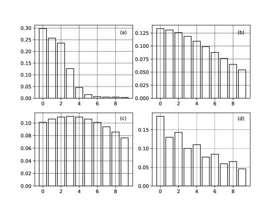
To the best of our knowledge the class of distributions (3) was not discussed by other authors. The corresponding class of distributions for the case $N=\infty$ is discussed in Appendix A. Several shapes of the distributions from the class (3) can be seen in Fig. 3 (note that the classes of distributions (3) and (3.10) are closely connected).

We note that the system of equations (3.4) - (3.6) is connected to the system of equations

$$x_{i}=F_{i}x_{i-1},i=1,\dots,N$$ (3.9)

where $F_{i}$ is a function of $i$ and eventually also a function of other variables and parameters. This connection can be easily proved. Let $f_{0}=\mu_{0}+\gamma_{0}-\sigma_{0}-\epsilon_{0}$ and we choose $f_{i}=\frac{f_{i-1}}{F_{i}}-\mu_{i}-\gamma_{i}+\sigma_{i}+\epsilon_{i}$; $i=1,\dots,N-1$; and $\gamma_{N}=\frac{f_{N-1}}{F_{N}}-\mu_{n}+\sigma_{N}+\epsilon_{n}$. Then Eq.(3.4) is satisfied and Eqs.(3.5) and (3.6) are transformed to Eq.(3.9).

Figure 2: Members of the family of truncated distributions (3.10) for the case of chain consisting of 10 urns. Horizontal axis - $k$. Vertical axis: probability $p(k)$. Figure (a): $F_{i}=2-\sin(i)$. Figure (b): $F_{i}=\exp(-0.02i)$ Figure (c): $F_{i}=1.07-\tanh(0.02i)$. Figure (d): $F_{i}=0.9+0.2(-1)^{i}$.

Eq.(3.9) leads to a class of statistical distributions as follows. From Eq.(3.9) we obtain $x_{i}=x_{0}\prod\limits_{k=1}^{i}F_{k}$ and then the amount of substance in the chain of urns will be $x=x_{0}\left[1+\sum\limits_{i=1}^{N}\prod\limits_{k=1}^{i}F_{k}\right]$. We can consider the statistical distribution $y_{i}=x_{i}/x$ of the amount of substance along the urns of the chain of urns. $y_{i}$ can be considered as probability values of distribution of a discrete random variable $\zeta$: $y_{i}=p(\zeta=i)$, $i=0,\dots,N$. For this distribution we obtain

$$y_{0}=\frac{1}{1+\sum\limits_{l=1}^{N}\prod\limits_{k=1}^{l}F_{k}};\ \ y_{i}=\frac{\prod\limits_{k=1}^{i}F_{k}}{1+\sum\limits_{l=1}^{N}\prod\limits_{k=1}^{l}F_{k}},\ i=1,\dots,N$$ (3.10)

The distribution (3.10) is closely connected to the distribution (3) as

$$F_{i}=\frac{f_{i-1}}{\mu_{i}+f_{i}+\gamma_{i}-\sigma_{i}-\epsilon_{i}};\ \ F_{N}=\frac{f_{N-1}}{\mu_{N}+\gamma_{N}-\sigma_{N}-\epsilon_{N}}.$$

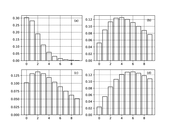
Because of the presence of the functions $F_{k}$ the shapes of the distributions from the class (3.10) (and the shapes of distributions from class (3) respectively) can be quite different one from another. Several shapes are shown in Fig.2. Appendix A contains the theory for the case $N=\infty$. The class of distributions (3.10) has many interesting particular cases. In Appendix A we show that for the case of infinite distributions the class of distributions (generated by the equations corresponding to Eq.(3) or Eq.(3.10) from the finite case discussed in the main text) contains as particular cases the Katz family of distributions, extended Katz family of distributions,Sundt and Jewell family of distributions, Ord family of distributions, and Kemp family of distributions.

Figure 3: Members of Kemp family of truncated distributions for a chain of 10 urns. Case $p=3$, $q=2$ in Eq.(A.15). Horizontal axis - $k$. Vertical axis: probability $p(k)$. Figure (a): $\lambda=0.4$, $a_{1}=0.8$, $a_{2}=0.7$, $a_{3}=1.2$, $b_{1}=0.6$, $b_{2}=0.3$, $b_{2}=0.4$. Figure (b): The values of the parameters are the same as in Figure (a) except for the value of the parameter $\lambda$ that is $\lambda=0.75$. The effect of increasing value of $\lambda$ is increasing the probability at the tail of the distribution. Figure (c): The values of the parameters are the same as in Figure (b) except for the value of the parameter $b_{3}$ which is $b_{3}=0.9$. The effect of the increasing value of $b_{1}$ is opposite to the effect of increasing value of $\lambda$ from Figure (b). Figure (d): The values of the parameters are the same as in Figure (b) except for the value of the parameter $a_{1}$ which is $a_{1}=1.4$.

These families contain numerous named distributions and some of them are listed in Appendix A. Here in the main text we consider the case of finite $N$ and because of this we obtain families of truncated distributions. For the case of relationship corresponding to the Katz family of distributions [84],[85] the Katz family of truncated distributions is obtained

$$y_{k}=\frac{\alpha+\beta(k-1)}{k}y_{k-1},k=1,\dots,N;\ \ y_{0}=\frac{1}{1+\sum\limits_{j=1}^{N}\prod\limits_{l=1}^{j}\frac{\alpha+\beta(l-1)}{l}}$$ (3.11)

Above $F_{k}=\frac{\alpha+\beta(k-1)}{k}$, and $\alpha$ and $\beta$ are parameters. The restrictions on the parameters are $\alpha>0$, $\beta<1$ (as $\beta\geq 1$ does not yield a valid distribution). If $\alpha+\beta n<0$, then $p_{n+j}$ is understood to be equal to zero for all $j>0$.

Let $F_{k}=\frac{\alpha+\beta(k-1)}{\gamma+k-1}$, $k=1,\dots,N$. Then we obtain the extended Katz family of truncated distributions [86] given by

$$y_{k}=\frac{\alpha+\beta(k-1)}{\gamma+k-1}y_{k-1},k=1,\dots,N;\ \ y_{0}=\frac{1}{1+\sum\limits_{j=1}^{N}\prod\limits_{l=1}^{j}\frac{\alpha+\beta(l-1)}{\gamma+l-1}}$$ (3.12)

In Eq.(3.12) $\alpha>0$, $\beta<1$ and $\gamma>0$. The resulting distribution will be named truncated hyper-negative binomial distribution as the corresponding distribution for $N=\infty$ has the name hyper-negative binomial distribution [87]. When $\beta\to 0$ in Eq.(3.12) we obtain a distribution we shall call truncated hyper-Poisson distribution because the corresponding distribution for the case $N=\infty$ was called hyper-Poisson distribution [88].

Another particular case of the distribution (3.10) is the Sundt and Jewell family of truncated distributions named after the corresponding family of distributions for the case $N=\infty$ [89], [90]. This family of distributions is obtained when

$$F_{k}=a+\frac{b}{k},k=1,\dots,N;\ \ y_{0}=\frac{1}{1+\sum\limits_{j=1}^{N}\prod\limits_{l=1}^{j}\left(a+\frac{b}{l}\right)}$$ (3.13)

Above $a$ and $b$ are parameters.

The Ord’s family of truncated distributions named after the Ord’s family of distributions [91] - [93] is obtained when

$$F_{k} = \frac{[(a+b_{0})+(b_{1}-1)k+b_{2}k(k-1)]-(k-a)}{(a+b_{0})+(b_{1}-1)k+b_{2}k(k-1)},k=1,\dots,N$$

$$y_{0} = \frac{1}{1+\sum\limits_{j=1}^{N}\prod\limits_{l=1}^{j}\frac{[(a+b_{0})+(b_{1}-1)l+b_{2}l(l-1)]+(l-a)}{(a+b_{0})+(b_{1}-1)l+b_{2}l(l-1)}}$$ (3.14)

In (3) $a$ and $b_{k}$ are parameters.

Finally we note that the Kemp’s family of truncated distributions named after Kemp’s family of distributions for the case $N=\infty$ [85], [94] is also a particular case of the the family of distributions (3.10) when

$$F_{k} = \frac{\lambda(a_{1}+k)\dots(a_{p}+k)}{(b_{1}+k)\dots(b_{q}+k)(b_{q+1}+k)},k=1,\dots,N$$

$$y_{0} = \frac{1}{1+\sum\limits_{j=1}^{N}\prod\limits_{l=1}^{j}\frac{\lambda(a_{1}+l)\dots(a_{p}+l)}{(b_{1}+l)\dots(b_{q}+l)(b_{q+1}+l)}}$$ (3.15)

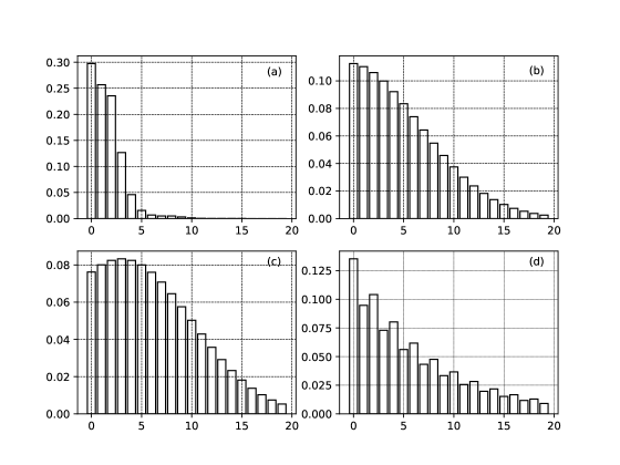
In (3) $\lambda$, $a_{i}$ and $b_{i}$ are parameters. Several members of the Kemp family of truncated distributions are shown in Fig. 3.

4 Concluding remarks

We discuss in this article a model of motion of substance in a chain of urns with possibility for exchange of substance among the chain of urns, the surrounding network and the environment of this network. Our attention was focused on the analytical results connected to this urn model. Such analytical results can be obtained, e.g., for the case of stationary motion of the substance through the chain of urns. For the case of infinite length of the chain of urns we obtain a family of discrete distributions that contains as particular cases many other families of discrete distributions, e.g., the families of distributions of Katz, Ord, and Kemp (see the Appendix). We write several characteristic quantities of the obtained family of distributions, e.g., mean and standard deviation. For the case of finite length of the chain of urns we obtain a family of distributions that are the truncated version of the discrete distributions of the family of distributions obtained for the case of chain of urns of infinite length. In analogy to the case of infinite chain of urns we name some subfamilies of distributions for the case of finite chain of urns as Katz, Ord, Kemp, etc. families of truncated distributions.

The discussed urn model has different practical applications. Let us discuss briefly just one of these applications: motion of migrants through a migration channel. In this case the chain of urns corresponds to the chain of countries that form the migration channel. The substance that is presented in the urns and moves between them corresponds to the migrants that move between the countries of the migration channel. The pumping process corresponds to inflow of migrants in the countries of the channel. This inflow can come from the network (countries from the same continent where the migration channel is positioned) or from the environment of the network (corresponding to the countries from the other continents). The process of leakage corresponds to outflow of migrants from the channel. This outflow can be to the countries from the continent where the channel is positioned (leakage to the network). The outflow can be also to the countries from other continents (outflow to the environment of the network). The obtained family of distributions corresponds to the distribution of migrants along the countries of the migration channel for the case of stationary regime of motion of migrants in the migration channel.

Appendix A Statistical distributions of substance for the case of chain of urns containing infinite number of urns

The model of infinite chain of urns corresponding to the model of finite chain of urns described by by Eqs.(3.1) - (3.3) is

$$\bigg{[}\sigma_{0}(t_{k})-\mu_{0}(t_{k})-f_{0}(t_{k})-\gamma_{0}(t_{k})+\epsilon_{0}(t_{k})\bigg{]}x_{0}(t_{k})=0,$$ (A.1)

$$\bigg{[}\mu_{i}(t_{k})+f_{i}(t_{k})+\gamma_{i}(t_{k})-\sigma_{i}(t_{k})-\epsilon_{i}(t_{k})\bigg{]}x_{i}(t_{k})=f_{i-1}(t_{k})x_{i-1}(t_{k}),$$

$$i=1,\dots,\infty.$$ (A.2)

Let us consider the case when the parameters of the model are time independent (i.e., when $\sigma_{i}(t_{k})=\sigma$; $\mu_{i}(t_{k})=\alpha_{i}$, $i=0,\dots,N$; $\gamma_{i}(t_{k})=\gamma_{i}$; $\epsilon_{i}(t_{k})=\epsilon_{i}$; $f_{0}(t_{k})=f_{0}$; $i=0,\dots,N$). In this case the system of model equations becomes

$$\bigg{[}\sigma_{0}-\mu_{0}-f_{0}-\gamma_{0}+\epsilon_{0}\bigg{]}x_{0}=0$$ (A.3)

$$\bigg{[}\mu_{i}+f_{i}+\gamma_{i}-\sigma_{i}-\epsilon_{i}\bigg{]}x_{i}=f_{i-1}x_{i-1},\ \ i=1,\dots,\infty$$ (A.4)

From Eqs. (A.3) and (A.4) we obtain the relationships

$$f_{0} = \sigma_{0}-\mu_{0}-\gamma_{0}+\epsilon_{0};$$

$$x_{i} = x_{0}\prod\limits_{k=1}^{i}\frac{f_{k-1}}{\mu_{k}+f_{k}+\gamma_{k}-\sigma_{k}-\epsilon_{k}},$$

From Eqs. (A) we obtain

$$x = \sum\limits_{l=0}^{\infty}x_{l}=x_{0}\Bigg{[}1+\sum\limits_{l=1}^{\infty}\prod\limits_{k=1}^{l}\frac{f_{k-1}}{\mu_{k}+f_{k}+\gamma_{k}-\sigma_{k}-\epsilon_{k}}\Bigg{]}$$ (A.6)

We can consider the statistical distribution $y_{i}=x_{i}/x$ of the amount of substance along the urns of the sequence of urns. $y_{i}$ can be considered as probability values of distribution of a discrete random variable $\zeta$: $y_{i}=p(\zeta=i)$, $i=1,\dots,\infty$. For this distribution we obtain

$$y_{0} = \frac{1}{1+\sum\limits_{l=1}^{\infty}\prod\limits_{k=1}^{l}\frac{f_{k-1}}{\mu_{k}+f_{k}+\gamma_{k}-\sigma_{k}-\epsilon_{k}}}$$

$$y_{i} = \frac{\prod\limits_{k=1}^{i}\frac{f_{k-1}}{\mu_{k}+f_{k}+\gamma_{k}-\sigma_{k}-\epsilon_{k}}}{1+\sum\limits_{l=1}^{\infty}\prod\limits_{k=1}^{l}\frac{f_{k-1}}{\mu_{k}+f_{k}+\gamma_{k}-\sigma_{k}-\epsilon_{k}}},\ \ i=1,\dots,\infty$$ (A.7)

To the best of our knowledge the class of distributions (A) was not discussed by other authors.

Note that the above parameters don’t depend on the time but they can depend on $i$ and on other parameters. Eqs. (A.3) and (A.4) are connected to the equation

$$x_{i}=F_{i}x_{i-1},i=1,\dots,\infty$$ (A.8)

where $F_{i}$ is a function of $i$ and eventually also a function of other variables and parameters. This connection can be easily shown. Let $f_{0}=\mu_{0}+\gamma_{0}-\sigma_{0}-\epsilon_{0}$; $f_{i}=\frac{f_{i-1}}{F_{i}}-\mu_{i}-\gamma_{i}+\sigma_{i}+\epsilon_{i}$;  $i=1,\dots,$. Then Eq.(A.3) is satisfied and Eq.(A.4) is transformed to Eq.(A.8). Eq.(A.8) leads to a class of statistical distributions as follows. From Eq.(A.8) we obtain $x_{i}=x_{0}\prod\limits_{k=1}^{i}F_{k}$ and then the amount of substance in the chain of urns will be $x=x_{0}\left[1+\sum\limits_{l=1}^{\infty}\prod\limits_{k=1}^{l}F_{k}\right]$.

We can consider the statistical distribution $y_{i}=x_{i}/x$ of the amount of substance along the urns of the sequence of urns. $y_{i}$ can be considered as probability values of distribution of a discrete random variable $\zeta$: $y_{i}=p(\zeta=i)$, $i=1,\dots,\infty$. For this distribution we obtain

$$y_{0}=\frac{1}{1+\sum\limits_{l=1}^{\infty}\prod\limits_{k=1}^{l}F_{k}};\ \ y_{i}=\frac{\prod\limits_{k=1}^{i}F_{k}}{1+\sum\limits_{l=1}^{\infty}\prod\limits_{k=1}^{l}F_{k}},\ i=1,\dots,\infty$$ (A.9)

We can write Eq.(A.8) as follows

$$y_{i}=F_{i}y_{i-1}$$ (A.10)

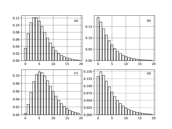
(Note that $F_{i}=\frac{f_{i-1}}{\mu_{i}+f_{i}+\gamma_{i}-\sigma_{i}-\epsilon_{i}}$ for the case of distribution (A)). Several members of the family of distributions (A.9) are shown in Fig. 10.

Figure 4: Members of the family of distributions (A.9). Horizontal axis - $k$. Vertical axis: probability $p(k)$. Figure (a): $F_{i}=2-\sin(i)$. Figure (b): $F_{i}=\exp(-0.02i)$ Figure (c): $F_{i}=1.07-\tanh(0.02i)$. Figure (d): $F_{i}=0.9+0.2(-1)^{i}$.

Particular case of the distributions defined by Eq.(A.10) is the Katz family of distributions [84]

$$y_{k}=\frac{\alpha+\beta(k-1)}{k}y_{k-1},\ \ k=1,\dots$$ (A.11)

Above $F_{k}=\frac{\alpha+\beta(k-1)}{k}$, and $\alpha$ and $\beta$ are parameters. The restrictions on the parameters are $\alpha>0$, $\beta<1$ (as $\beta\geq 1$ does not yield a valid distribution). If $\alpha+\beta n<0$, then $p_{n+j}$ is understood to be equal to zero for all $j>0$. The Katz family of distributions contains the following important distributions [84], [85]:

• Binomial distribution : For $\beta<0$ one obtains the binomial distribution with $\alpha=\frac{nq}{p}$, $\beta=-\frac{q}{p}$,

• Poisson distribution: It is obtained when $\beta=0$ and $\alpha=\theta$,

• Negative binomial distribution: It is obtained when $0<\beta<1$ and $\alpha=\frac{jP}{P+1}$; $\beta=\frac{P}{P+1}$.

The three distributions above are particular cases of the class of distributions defined by Eq.(A.10).

Let $F_{k}=\frac{\alpha+\beta(k-1)}{\gamma+k-1}$, $k=1,\dots$. Then we obtain the extended Katz family of distributions [86] given by

$$y_{k}=\frac{\alpha+\beta(k-1)}{\gamma+k-1}y_{k-1},\ \ k=1,\dots$$ (A.12)

In Eq.(A.12) $\alpha>0$, $\beta<1$ and $\gamma>0$. The resulting distribution was called hyper-negative binomial distribution [87]. When $\beta\to 0$ in Eq.(A.12) one obtains the hyper-Poisson distribution [88]. Several members of the Katz family of distributions and extended Katz family of distributions are shown in Fig.11.

Figure 5: Members of Katz family of distributions (Figures (a) and (b)) and of extended Katz families of distributions (Figures (c) and (d)). Horizontal axis - $k$. Vertical axis: probability $p(k)$. Figure (a): $\alpha=2.2$, $\beta=0.6$. Figure (b): $\alpha=0.9$, $\beta=0.75$. Figure (c): a member of the extended Katz family of distributions. The values of $\alpha$ and $\beta$ are the same as in Figure (a). The additional parameter $\gamma$ of the extended Katz family of distributions has value $\gamma=0.3$. The presence of the parameter $\gamma$ leads to increasing probability in the tail of the distribution and to change of the shape of distribution. Figure (d): another member of the extended Katz family of distributions. Values of parameters $\alpha$ and $\beta$ are the same as in Figure (b). The value of parameter $\gamma$ is $\gamma=0.8$.

Another particular case of (A.10) is the Sundt and Jewell family of distributions. It is obtained when [89], [90]

$$F_{k}=a+\frac{b}{k},k=1,\dots.$$ (A.13)

The Ord’s family of distributions [91] - [93] is obtained when

$$F_{k}=\frac{[(a+b_{0})+(b_{1}-1)k+b_{2}k(k-1)]-(k-a)}{(a+b_{0})+(b_{1}-1)k+b_{2}k(k-1)}.$$ (A.14)

In (A.14) $a$ and $b_{k}$ are parameters. Ord obtained the following kinds of distributions: hypergeometric, negative hyper-geometric (beta-binomial), beta-Pascal, binomial, Poisson, negative binomial, discrete Student’s t. All these case of distributions from the Ord’s family of distributions are also particular cases of the lass of distributions (A.9).

Finally we note that the Kemp’s family of distributions (the generalized hypergeometric probability distributions) [85], [94] is also a particular case of the the family of distributions (A.9) when

$$F_{k}=\frac{\lambda(a_{1}+k)\dots(a_{p}+k)}{(b_{1}+k)\dots(b_{q}+k)(b_{q+1}+k)}.$$ (A.15)

In (A.15) $\lambda$, $a_{i}$ and $b_{i}$ are parameters. Dacey [95] (see Table 2 there) lists 41 named distributions that belong to the Kemp’s family of distributions. Let us mention some of them as they are also particular cases of the class of distributions (A.9) (or (A)). The distributions we mention here are: Binomial distribution, Generalized Poisson Binomial distribution, Poisson distribution, Hyper-Poisson distribution, Geometric distribution, Pascal distribution, Negative Binomial distribution, Polya-Eggenberger distribution, Stirling distributions of first and second kind, Hypergeometric, Inverse Hypergeometric and Negative Hypergeometric distributions, Polya and Inverse Polya distributions, Hermite distribution, Neuman distribution of type A, B, and C, Waring distribution, Yule distribution.

References

- [1] R. Albert, A. -L. Barabasi. Rev. Mod. Phys. 74 (2002), 47 - 97
- [2] S. Boccaletti, V. Latora, Y. Moreno, M. Chavez, D. U. Hwang. Physics Reports 424 (2006) 175 - 308.
- [3] Z. I. Dimitrova, N. K. Vitanov. Journal of Physics A: Mathematical and General 34 (2001) 7459 - 7473
- [4] Z. I. Dimitrova, N. K. Vitanov. Physica A 300 (2001) 91 - 115
- [5] Z. I. Dimitrova, N. K.Vitanov. Theoretical Population Biology 66 (2004), 1 - 12.
- [6] E. V. Nikolova, V. K. Kotev, G. S. Nikolova. EMBEC & NBC 2017. IFMBE Proceedings 65, Springer, Singapore, 209 - 212 (2018).
- [7] E. V. Nikolova. AIP Conference Proceedings 1978 (2018), 470050.
- [8] T. B. Ivanov, E. V. Nikolova. Advanced Computing in Industrial Mathematics. Studies in Computational Intelligence 681, 61 - 74, Springer, Cham (2017).
- [9] E. Nikolova, T. Ivanov. Series on Biomechanics 29 (2015) 78 - 84
- [10] S. Tabakova, E. Nikolova, S. Radev. AIP Conference Proceedings 1629 (2014), 336 - 343.
- [11] E. Nikolova. Compt. rend. Acad. bulg. Sci. 65 (2012) 33 - 40.
- [12] V. Petrov, E. Nikolova, O. Wolkenhauer. IET Systems Biology 1 (2007) No. 1, 2 - 9
- [13] V. Petrov, E. Nikolova, J. Timmer. Journal of Theoretical and Applied Mechanics 34 (2004), 55 - 78
- [14] E. Nikolova, E. Goranova, Z. Dimitrova. Compt. rend. Acad. bulg. Sci. 69 (2016) 1213 - 1222
- [15] I. Jordanov, E. Nikolova. Journal of Theoretical and Applied Mechanics 43 (2013) 69 - 76
- [16] E. Nikolova, V. Petrov. Compt. rend. Acad. bulg. Sci. 63 (2010) 1421 - 1428
- [17] E. Nikolova, V. Petrov, I. Edissonov. Journal of Theoretical and Applied Mechanics 41 (2011), 83 - 92
- [18] I. Edissonov, E. Nikolova, S. Ranchev. Compt. rend. Acad. bulg. Sci. 61 (2008), 1401 - 1406
- [19] E. Nikolova. Compt. rend. Acad. bulg. Sci. 59 (2006) 143 - 150
- [20] E. V. Nikolova, J. Timmer, V. G. Petrov. Series on Biomechanics 24 (2009),79 - 100
- [21] Z.I. Dimitrova. M. Ausloos. Open Physics 13 (2015) 218 - 225
- [22] N. K. Vitanov, M. Ausloos. Journal of Applied Statistics 42 (2015) 2686 - 2693
- [23] Z. I. Dimitrova. Journal of Theoretical and Applied Mechanics 45 (2015), 79 - 92
- [24] M. Ausloos, A. Gadomski, N. K. Vitanov. Physica Scripta 89 (2014), 108002
- [25] K. Vitanov, M. Slavtchova-Bojkova. Annual of Sofia University ”St. Kliment Ohridski”, Faculty of Mathematics and Informatics 104 (2018) 193 - 200
- [26] N. K. Vitanov, Z. I. Dimitrova. Communications in Nonlinear Science and Numerical Simulation 15 (2010) 2836 - 2845
- [27] N. K. Vitanov, Z. I. Dimitrova, H. Kantz. Applied Mathematics and Computation 216 (2010) 2587 - 2595
- [28] N. K. Vitanov, Z. I. Dimitrova, K. N. Vitanov. Applied Mathematics and Computation 269 (2015) 363 - 378
- [29] Z. Dimitrova. Journal of Theoretical and Applied Mechanics 42, No. 3 (2012) 3 – 22
- [30] I. P. Jordanov. Compt. rend. Acad. bulg. Sci. 61 (2008) 307 - 314
- [31] N. K. Vitanov, M. Ausloos. Knowledge epidemics and population dynamics models for describing idea diffusion, pp. 69 - 125 in Models of science dynam-ics, edited by A. Scharnhorst, K. Börner, P. van den Besselaar. Berlin, Springer, 2012
- [32] B. Li, J. Springer, G. Bebis, M. H. Gunes. Journal of Network and Computer Applications 36 (2013) 567 - 581
- [33] M. Eboli. Financial applications of flow network theory. pp. 21 - 29 in A. N. Proto, M. Squillante, J. Kacprzyk (Eds.). Advanced Dynamics modeling of economic and social systems. Springer, Berlin, pp. 2-13.
- [34] W. -K. Chen. Flows in networks. Imperial College Press, London, 2003.
- [35] L. D. Ford, Jr., D. R. Fulkerson. Flows in networks. Princeton University Press, Princeton, NJ, 1962.
- [36] V Tejedor, O Benichou, R Voituriez. Phys. Rev. E 83 (2011) 066102.
- [37] W.-K. Chan. Theory of nets: Flows in networks. Wiley, New York, 1990.
- [38] G. Ruhe. Algorithmic aspects of flows in networks. Springer, Netherlands, 1991.
- [39] M. T. Todinov. Flow networks. Analysis and optimization of repairable flow networks, networks with disturbed flows, static flow networks and reliability networks. Elsevier, Amsterdam, 2013.
- [40] L. Ambrosio, A. Bressan, D. Helbing, A. Klar, E. Zuazua (Eds.). Modeling and optimisation of flows on networks. Springer, Heidelberg, 2010.
- [41] N. H. Gartner, G. Improta (Eds.) Urban traffic networks. Dynamic flow modeling and control. Springer, Berlin, 1995.
- [42] E. Bernard, L. Jacob, J. Mairal, J.-P. Vert. Bioinformatics 30 (2014) 2447 – 2455.
- [43] M. Rossvall, A.C. Esquivel, A. Lancichinetti, J. D. West, R. Lambiotte. Memory in network flows and its effects on spreading dynamics and community detection. Nature Communications 5 (2014) Article No. 4630.
- [44] G. Masson, B. W. Jordan, Jr. Networks 2 (1972) 191 - 209.
- [45] W. C. Jordan, M. A. Turnquist. Transportation Science 17 (1983), 123 - 145.
- [46] D. Helbing, L. Buzna, A. Johansson, T. Werner. Transportation Science 39 (2005) 1 - 24.
- [47] J. E. Aronson. Annals of Operation Research 20 (1989) 1 - 66.
- [48] M. Treiber, A. Kesting. Traffic flow dynamics: Data, models, and simulation. Springer, Berlin, 2013.
- [49] M. Skutella. An introduction to network flows over time. pp. 451 - 482 in W. Cook, L. Lovasz, J. Vygen (Eds.) Research trends in combinatorial optimization. Springer, Berlin, 2009.
- [50] N. K. Vitanov, K. N. Vitanov. Physica A 509 (2018) 635-650.
- [51] F. J. Willekens. SA Journal of Demography 7 (1999) 31 - 43.
- [52] H. -P. Blossfeld, G. Rohwer. Techniques of event history modeling: new approaches to casual analysis. Lawrence Erlbaum, New Jersey, 2002.
- [53] D. S. Hachen. Sociological Methods and Research 17 (1988) 21 - 54.
- [54] J. Raymer. Environment and Planning A 39 (2007) 985 - 995.
- [55] M. J. Greenwood. Modeling migration, in K. Kemp-Leonard, (Ed.) Encyclopedia of social measurement, vol. 2, Elsevier, Amsterdam, 2005, pp. 725 - 734.
- [56] E. S. Lee. Demography 3 (1966) 47 - 57.
- [57] R. Armitage. Population Trends 43 (1986) 31-40.
- [58] I. Bracken, J. J. Bates. Environment and Planning A 15 (1983) 343-355.
- [59] J. R. Harris, M. P. Todaro. The American Economic Review 60 (1970) 126 - 142.
- [60] J. H. Simon. The economic consequences of migration. The University of Michigan Press, Ann Arbor, MI, 1999.
- [61] G. J. Borjas. International Migration Review 23 (1989) 457 - 485.
- [62] J. T. Fawcet. International Migration Review 23 (1989) 671 - 680.
- [63] D. T. Gurak, F. Caces. Migration networks and the shaping of migration systems. pp. 150 - 176 in M. M. Kitz, L. L. Lim, H. Zlotnik (Eds.) International migration systems: A global approach. Clarendon Press, Oxford, 1992.
- [64] N. K. Vitanov, K. N. Vitanov. Mathematical Social Sciences 80 (2016) 108 - 114
- [65] N. K. Vitanov, K. N. Vitanov, T. Ivanova. Box model of migration in channels of migration networks, in Advanced Computing in Industrial Mathematics, edited by K. Georgiev et al., Studies in Computational Intelligence No. 728, Springer, Berlin, (2018), pp. 203 - 215.
- [66] N. K. Vitanov, R. Borisov. Journal of Theoretical and Applied Mechanics 48, No. 3 (2018) 74 - 84.
- [67] N. K. Vitanov, R. Borisov. Statistical characteristics of a flow of Substance in a channel of network that contains three arms. in: Georgiev K., Todorov M., Georgiev I. (eds.). Advanced Computing in Industrial Mathematics. BGSIAM 2017. Studies in Computational Intelligence, vol 793. Springer, Cham (2018), pp. 421 - 432.
- [68] N. K. Vitanov, K. N. Vitanov. Physica A 490 (2018) 1277 - 1294.
- [69] N. K. Vitanov, Z. I. Dimitrova, M. Ausloos. Physica A 389 (2010) 4970 - 4980.
- [70] N. K. Vitanov, M. Ausloos, G. Rotundo. Advances in Complex Systems 15, Supplement 1 (2012) Article number 1250049.
- [71] N. K. Vitanov, I. P. Jordanov, Z. I. Dimitrova. Communications in Nonlinear Science and Numerical Simulation 14 (2009) 2379 - 2388.
- [72] N. K. Vitanov, I. P. Jordanov, Z. I. Dimitrova. Applied Mathematics and Computation 215 (2009) 2950 - 2964.
- [73] N. K. Vitanov, Z. I. Dimitrova, K. N. Vitanov. Computers & Mathematics with Applications 66 (2013) 1666 - 1684.
- [74] N. K. Vitanov, K. N. Vitanov. Computers & Mathematics with Applications 68 (2013) 962 - 971.
- [75] A. Schubert, W. Glänzel. Scientometrics 6 (1984) 149 – 167.
- [76] N. K. Vitanov. Science dynamics and research production. Indicators, Indexes, statistical laws, and mathematical models. Springer, Cham, 2016.
- [77] N. Johnson, S. Kotz. Urn models and their applications. An approach to modern discrete probability theory. New York, Wiley, 1977.
- [78] G. H. Weiss. Biometrics, 21 (1965) 481 - 490.
- [79] K. Dietz. Journal of Applied Probability, 3 (1966) 375 - 382.
- [80] P. Clifford, A. Sudbury. Biometrika, 60 (1973) 581 - 588.
- [81] L. J. Wei. Journal of the American Statistical Association, 73 (1978) 559 - 563.
- [82] A. Bagchi, A. K. Pal. SIAM Journal on Algebraic Discrete Methods, 6 (1985) 394 - 405.
- [83] S. Boucheron, D. Gardy. Random Structures & Algorithms, 10 (1997) 43 - 67.
- [84] L. Katz. Unified treatment of a broad class of discrete probability distributions. In G. P. Patil (Ed.) Classical and Contagious Discrete Distributions. Statistical Publishing Society, Calcutta, 1965, pp. 175 - 182.
- [85] N. L. Johnson, A. W. Kemp, S. Kotz. Univariate discrete distributions. Wiley, Hoboken, New Jersey, 2005.
- [86] J. Gurland, R. C. Tripathi. Estimation of parameters on some extensions of the Katz family of discrete distributions involving hypergeometric functions. In G. P. Patil, S. Kotz, J. K. Ord (Eds.) Statistical distributions in scientific work, Vol. 1: Models and structures. Reidel, Dordrecht, 1975, pp. 59 - 82.
- [87] M. A. Yousry, R. C. Srivastava. Biometrical Journal, 29 (1987) 875 - 884.
- [88] G. E. Bardwell, E. L. Crow. Journal of the American Statistical Association 59 (1964) 133 - 141.
- [89] B. Sundt, W. S. Jewell. ASTIN Bulletin, 18 (1981) 27 - 39.
- [90] G. E. Willmot. ASTIN Bulletin, 18, (1988) 17 – 29.
- [91] J. K. Ord. Journal of the Royal Statistical Society, Series A, 130 (1967) 232 - 238.
- [92] J. K. Ord. Biometrika, 54 (1967) 649 - 656.
- [93] J. K. Ord. Families of frequency distributions. London, Griffin, 1972.
- [94] A. W. Kemp. Sankhya, Series A, 30 (1968) 401 - 410.
- [95] M. F. Dacey. Sankhya, Series B, 34 (1972) 243 - 250.