Group connectivity in COSMOS: a tracer of mass assembly history

Abstract

Cosmic filaments are the channel through which galaxy groups assemble their mass. Cosmic connectivity, namely the number of filaments connected to a given group, is therefore expected to be an important ingredient in shaping group properties.
The local connectivity is measured in COSMOS around X-Ray detected groups between redshift 0.5 and 1.2. To this end, large-scale filaments are extracted using the accurate photometric redshifts of the COSMOS2015 catalogue in two-dimensional slices of thickness 120 comoving Mpc centred on the group’s redshift. The link between connectivity, group mass and the properties of the brightest group galaxy (BGG) is investigated. The same measurement is carried out on mocks extracted from the lightcone of the hydrodynamical simulation Horizon-AGN in order to control systematics.
More massive groups are on average more connected. At fixed group mass in low-mass groups, BGG mass is slightly enhanced at high connectivity, while in high mass groups BGG mass is lower at higher connectivity. Groups with a star-forming BGG have on average a lower connectivity at given mass. From the analysis of the Horizon-AGN simulation, we postulate that different connectivities trace different paths of group mass assembly: at high group mass, groups with higher connectivity are more likely to have grown through a recent major merger, which might be in turn the reason for the quenching of the BGG. Future large-field photometric surveys, such as Euclid and LSST, will be able to confirm and extend these results by probing a wider mass range and a larger variety of environment.

1 Introduction

In the local Universe, a large fraction of the stellar mass resides in galaxy groups and clusters. These environments are the place of a wide variety of quenching processes, mostly depending on the group mass, leading to different galaxy population contents (e.g. Gobat et al., 2015; Treyer et al., 2018). These processes are first connected to the availability and physical state of the intra-cluster gas. The infalling cold gas can be gravitationally heated (e.g. Birnboim & Dekel, 2003; Kereš et al., 2005), maintained hot via feedback from Active Galaxy Nuclei (AGN, Dubois et al., 2013), and therefore not available anymore for accretion and star formation. Other processes are related to interactions between gas and galaxies, such as ram-pressure stripping (Gunn & Gott, 1972), or between galaxies, including galaxy mergers, galaxy harassment (Moore et al., 1996) or tidal interactions (Byrd & Valtonen, 1990). In addition, the infalling gas in the group or cluster can be diverted towards the central galaxy or its satellites, depending on their relative mass (e.g. Simha et al., 2009) and the relaxation state of the group, a process often leading to satellite quenching by starvation (e.g. van de Voort et al., 2017) due to tidal effect in the neighbourhood of the most massive galaxy.

Groups are not isolated structures but they keep accreting matter – including small galaxies, but also gas (Kauffmann et al., 2010) – from the large-scale cosmic web they are connected to. Therefore, investigating the link between the large-scale cosmic web and group properties is an essential question for galaxy formation but also cosmology. On the one hand, the mean number of filaments branching out from groups – namely their local connectivity – depends on the growth factor and therefore the Dark Energy equation of state. Precise measurement of this quantity provides a topologically robust alternative to constrain cosmology, as it can be shown to depend on moments of the hierarchy of the N-point correlation functions (Codis et al., 2018). The disconnection of filaments with cosmic time is driven both by gravitational clustering and by dark energy which will stretch and disconnect neighbouring filaments through the increased expansion of voids.

On the other hand, the geometry and anisotropy of the large-scale environment is connected to the nature, history and dynamics of matter infall, knowledge of which, in turn, is essential to shape the mass assembly of groups and clusters. Several works have already emphasized the link between the large-scale environment and the properties of groups and their central galaxies (e.g. Scudder et al., 2012; Luparello et al., 2015; Zehavi et al., 2018), although some others conclude on the absence of correlation for high-mass halos (Jung et al., 2014). The variety of definitions for the large-scale environment can be one of the reasons for these conflicting conclusions. On a similar note, the measured correlation between the quenching of the central galaxy and the fraction of quenched satellites in the group, introduced as ’galactic conformity’ by Weinmann et al. (2006), and either confirmed or debated since then (e.g. Kauffmann et al., 2013; Hearin et al., 2016; Hartley et al., 2015; Treyer et al., 2018), can be interpreted as an environmental process, in which the properties of both central and satellite galaxies of a given group depend on the mass assembly history of their host halo, which depends on the large-scale environment. In fact, the geometry of matter infall on groups being for the most part filamentary, this environmental question must be addressed primarily from the perspective of the cosmic web. Several questions are still unanswered: where do the groups sit in the cosmic web as a function of their mass? Can the filaments penetrate deeply into halos and preferentially feed the central galaxies, or are the satellites bringing in all the accreted gas? What fraction of the mass load and the angular momentum is advected by how many filaments (e.g. Pichon et al., 2011; Tillson et al., 2011; Danovich et al., 2012, 2015)? Can we understand cosmic connectivity as a function of the rareness of the nodes and prominence of filaments? How is (stellar or AGN) feedback impacted by the number of connected filaments? Observationally, detecting filaments around groups is an essential first step to address these questions.

This quest has therefore raised the interest of many and is now a growing field of investigation, with various methods of filament detections, including weak lensing (Dietrich et al., 2005; Jauzac et al., 2012; Gouin et al., 2017), stacking thermal Sunyaev-Zel’dovich detection (Bonjean et al., 2018) or galaxy overdensity (Zhang et al., 2013) between clusters pairs, X-Ray emission (Dietrich et al., 2012; Parekh et al., 2017) or measurement of the local elongation spotted in the galaxy density distribution (Darvish et al., 2015; Durret et al., 2016). Beyond trying to understand the process of mass assembly in the largest virialized structures of the Universe, the motivation for hunting matter in filaments is also to create a comprehensive census of the baryonic matter in the Universe. Although these first detections are encouraging, a more systematic study is needed in order to draw statistically significant conclusions on the impact of the large-scale environment on galaxy group properties. These studies require a complete catalogue of accurate galaxy redshifts in order to precisely identify filaments, and a volume large enough to host both a significant number of massive structures and a large variety of large-scale environments. Large spectroscopic surveys are promising for this purpose, but are for now limited to low redshift (see e.g. Poudel et al., 2017, for a study in the SDSS). An alternative is to rely on photometric data. As shown in Laigle et al. (2018), filaments can be reliably extracted from photometric redshifts by relying on two-dimensional slices, the thickness of which is calibrated based on the typical redshift accuracy. As an example, extracting filaments from photometric redshifts around massive clusters has been already successfully done in the CFHTLS T0007 data (Sarron et al., 2019) at low redshift ($0.15<z<0.70$).

In this work, we rely on the wealth of photometric data from the COSMOS field to perform the filament extraction around intermediate-mass groups at higher redshift, and we make use of a robust group catalogue which has been extracted from X-Ray photometry (Finoguenov et al., 2007; Gozaliasl et al., 2019). The correlation between group connectivity, group mass and the BGG properties is first quantified both in the observations and the corresponding mocks. In the second step, the Horizon suite (Dubois et al., 2014) is used to interpret the observational results. The paper is organised as follows. Section 2 describes the observed and simulated datasets and the tools used to extract the skeleton. Section 3 presents the measurements both from the observed and simulated catalogues, and an extensive assessment of the robustness of the results. Section 4 provides an interpretation of the observational results based on the Horizon-AGN simulation. Section 5 summarizes the results and outlines future works. Appendix A gives more details on the connectivity measurement in the simulation and in COSMOS. We use a standard $\Lambda$CDM cosmology with a Hubble constant $H_{0}=70.4$ km$\cdot$s${}^{-1}\cdot{\rm Mpc}^{-1}$, total matter density $\Omega_{\rm m}=0.272$ and dark energy density $\Omega_{\Lambda}=0.728$. Unless specified otherwise, errorbars are the errors on the mean derived from bootstrap resampling.

2 Dataset and extraction methods

Let us first present briefly the observational dataset, the simulations and the ridge extraction tools used to quantify the connectivity of groups, and the robustness of this extraction with respect to photometric redshift uncertainty.

2.1 The COSMOS dataset

The analysis presented here is based on the COSMOS dataset (Scoville et al., 2007). The cosmic web is extracted using the photometric redshift of the COSMOS2015 catalogue (Laigle et al., 2016), which is also used for deriving galaxy masses. Groups are extracted from the X-Ray photometry as described in Finoguenov et al. (2007) and Gozaliasl et al. (2019). The observed catalogue of groups, their associated BGG and filaments in COSMOS is called $\mathscr{C}_{\rm cosmos}$ in the following analysis.

Name	Data	Group selection	$z$ and mass ranges	CW extraction and persistence	comments
$\mathscr{C}_{\rm cosmos}$	COSMOS field	X-Ray	0.5$<z<$1.2	in 2D slices (120Mpc), 1.5$\sigma$	photo-$z$ and
	1.38 deg2	86 groups	13.38 $<\log M_{\rm group}/{\rm M}_{\odot}$	from galaxies, $M_{*}>10^{10}{\rm M}_{\odot}$	masses
$\mathscr{C}_{\rm Hzagn\,2D}^{\rm phot}$	Horizon-AGN ligthcone	AdaptaHOP	0.5$<z<$1.2	in 2D slices (120Mpc), 1.5$\sigma$	photo-$z$ and
	1 deg2	76 groups	13.3 $<\log M_{\rm group}/{\rm M}_{\odot}$	from galaxies, $M_{*}>10^{10}{\rm M}_{\odot}$	masses
$\mathscr{C}_{\rm Hzagn\,2D}^{\rm true}$	Horizon-AGN ligthcone	AdaptaHOP	0.5$<z<$1.2	in 2D slices (120Mpc), 1.5$\sigma$	intrinsic-$z$
	1 deg2	76 groups	13.3 $<\log M_{\rm group}/{\rm M}_{\odot}$	from galaxies, $M_{*}>10^{10}{\rm M}_{\odot}$	and masses
$\mathscr{C}_{\rm Hzagn\,3D}$	Horizon-AGN snapshots	AdaptaHOP	3 snapshots, $z=0.63,\,0.81,\,1.03$	in 3D, 5$\sigma$	intrinsic-$z$
	$3\times 100^{3}$ (Mpc$/h$)3	1115 groups	13.0 $<\log M_{\rm group}/{\rm M}_{\odot}$	from all DM halos	and masses

Table 1: A summary of all the catalogues used in this study, the data selection, the group and CW extraction methods and the persistence thresholds used in DisPerSE.

2.1.1 COSMOS2015 redshifts and stellar masses

The COSMOS2015 catalogue provides apparent magnitudes in 30 bands from ultra-violet (UV) to infra-red (IR). The photometric data include the optical COSMOS-20 subaru survey (Capak et al., 2007; Ilbert et al., 2009), Subaru Suprime-Cam data (Taniguchi et al., 2007, 2015), the $u^{*}$-band data from the Canada-Hawaii-France Telescope (CFHT/MegaCam), NIR photometry from the UltraVISTA survey (DR2, McCracken et al., 2012), the $Y$ band from the Hyper Suprime-Cam at Subaru telescope (Miyazaki et al., 2012) and mid-IR data in the four IRAC channels (i.e. in a wavelength range between $\sim 3$ and $8\,\mu$m) from the SPLASH program (PI: Capak). Galaxy photometry in optical and NIR has been extracted using SExtractor (Bertin & Arnouts, 1996) in dual image mode, using as the detection image a $\chi^{2}$ sum of the four NIR images of UltraVISTA DR2 and the $z^{++}$-band (taken with Subaru Suprime-Cam). We removed from the catalogue all the objects which are flagged as belonging to a polluted area or for which the photometry is possibly contaminated by the light of saturated stars, meaning that only objects in $\cal{A}^{\rm UVISTA}$&$\cal{A}^{\rm!OPT}$&$\cal{A}^{\rm COSMOS}$ are kept, according to the notations in Table 7 of Laigle et al. (2016).

Photometric redshifts (photo-$z$), stellar masses and absolute magnitudes have been computed using LePhare (Arnouts et al., 2002; Ilbert et al., 2006) with a configuration similar to Ilbert et al. (2013). The stellar mass completeness of the sample is estimated from the $K_{\rm s}$ magnitude following Pozzetti et al. (2010). At redshift $z=1.2$, the sample is 90% complete down to $M_{\rm lim}=10^{9.2}{\rm M}_{\odot}$. However, in this work, only galaxies more massive than $10^{10}{\rm M}_{\odot}$ are used to extract the filament distribution over the redshift range $0.5<z<1.2$. Because our analysis relies on a global extraction of the filaments – in contrast to previous works which are based on a local search around groups –, a large enough comoving area is required, which sets the lower limit of our redshift range to $z\sim 0.5$. The upper limit is defined by the rapid increase of the redshift uncertainties at $z\sim 1.2$ (see Fig. 14 of Laigle et al., 2016).

A large spectroscopic redshift catalogue is also available on the COSMOS field, as the result of the common effort of several spectroscopic follow-up campaigns since 2007 (e.g. Lilly et al., 2007; Kartaltepe et al., 2010; Le Fèvre et al., 2015; Comparat et al., 2015). This spectroscopic sample is essential for the calibration of the photometric redshifts and for a better determination of group redshifts.

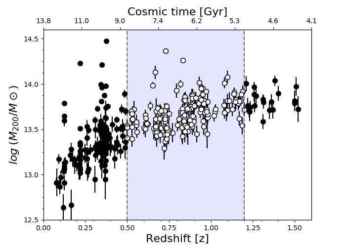
Figure 1: The halo mass of X-ray groups ($M_{200}$) in the COSMOS field as a function of redshift (filled and open circles). The highlighted area represents the groups with a redshift range of $0.5<z<1.2$, which is used in this study (open circles).

2.1.2 The X-Ray group catalogue

The initial catalogues of the X-Ray galaxy groups in COSMOS were presented in Finoguenov et al. (2007) and George et al. (2011). These catalogues combined the available Chandra and XMM-Newton data (with improvements in the photometric datasets) used for identification of galaxy groups, with confident identification reaching out to $z\sim 1.0$. The COSMOS galaxy group catalogue we rely on is a combination of an updated version of the initial group catalogues and a new catalogue of 73 groups described in Gozaliasl et al. (2019) and Gozaliasl et al. in preparation, which combines data of all X-ray observations from Chandra and XMM-Newton in the 0.5-2 keV band, with robust group identification up to $z\sim 1.53$. However, for the purpose of this study and for the reason explained above, we limit our selection to $z\sim 0.5-1.2$ (highlighted area in Fig. 1).

Group halo mass is the total mass (commonly called $M_{200}$, but we call it $M_{\rm group}$ in the rest of this paper), determined using the scaling relation $L_{X}-M_{200}$ with weak lensing mass calibration as presented by Leauthaud et al. (2010). The radius of the group $R_{200}$ is defined as the radius enclosing $M_{200}$ with a mean overdensity of $\Delta\sim 200$ times the critical background density. Fig. 1 presents the group mass $\log(M_{200}/{\rm M}_{\odot})$ as function of the redshift and cosmic time. Gozaliasl et al. (2019) discussed the mass completeness of the group sample given the surface brightness limitation of the X-Ray dataset. Over the redshift range $0.5<z<1.2$, the evolution of the group mass limit is weak and lies within the observational uncertainties, being around $\log M_{\rm group}/{\rm M}_{\odot}\sim 13.38$ at $z\sim 0.5$ and $\log M_{\rm group}/{\rm M}_{\odot}\sim 13.5$ at $z\sim 1.2$.

The redshift of the group is the redshift of the peak of the galaxy distribution within the group radius, while slicing the lightcone with a redshift step of 0.05. In most cases, this redshift determination is strengthened by the presence of spectroscopic redshifts. The brightest group galaxy (BGG in the following) is identified from the COSMOS2015 photometry as being the most massive galaxy within $R_{200}$, with a redshift that agrees with that of the hosting group (Gozaliasl et al., 2019). More than $\sim 80\%$ of the BGGs have secure spectroscopic redshifts. Group centers from the X-Ray emission are determined with an accuracy of $\sim 5\arcsec$, using the smaller scale emission detected by Chandra data. The BGG does not always sit at the peak of the X- Ray centre emission. As described in Gozaliasl et al. (2019), the off-central BGG probably reside in groups which are more likely to have experienced a recent halo merger.

As described in Gozaliasl et al. (2019), a quality flag has been assigned to each group depending on the robustness of the extraction and the potential availability of spectroscopic redshift. In our study, we keep only group with a flag of 1, 2, and 3. Over the redshift range $0.5<z<1.2$ and considering only groups with a BGG galaxies more massive than $\log M_{*}/{\rm M}_{\odot}=10$ and in a non-flagged area, we are left with 86 groups containing around 900 galaxies, over 1.38 deg² (or $\sim$62 groups per square degree).

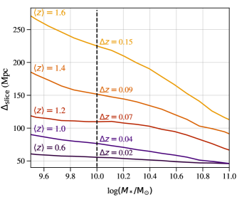
Figure 2: Minimal slice thickness $\Delta_{\rm slice}$ in comoving Mpc which has to be chosen in $\mathscr{C}_{\rm cosmos}$ for the purpose of cosmic web extraction in 2D, as a function of masses and for different redshifts (from $\langle z\rangle=1.6$ to $\langle z\rangle=0.6$, yellow to dark blue lines). Here $\Delta_{\rm slice}$ is the comoving thickness corresponding to $\Delta{z}=2\times 1\sigma_{z}$, where $\sigma_{z}$ is the redshift uncertainty of the lowest mass galaxies in the sample. Above each line is also indicated $\Delta{z}$ corresponding to the galaxies in the $10^{10}{\rm M}_{\odot}$ bin.

2.2 The Horizon-AGN simulation

The Horizon-AGN (Dubois et al., 2014) cosmological hydrodynamical simulation is used both to assess the quality of the observational measurements and to provide an interpretative framework. Therefore, several catalogues are built from the simulation. We first make use of the mock catalogue which has been generated from the Horizon-AGN simulated lightcone. Two versions of this catalogue are built: $\mathscr{C}_{\rm Hzagn\,2D}^{\rm phot}$ and $\mathscr{C}_{\rm Hzagn\,2D}^{\rm true}$, for which cosmic web filaments are extracted either from the photometric quantities (redshift and masses, Laigle et al., 2019) or intrinsic ones respectively. Comparing the results from these catalogues allows to quantify the impact of photometric noise and to assess the quality of the connectivity measurement from observations (Section 2.4).
Furthermore, in order to interpret the data (Section 4), and in particular to probe how AGN feedback comes into play, an additional catalogue is used: $\mathscr{C}_{\rm Hzagn\,3D}$, built from the Horizon-AGN snapshot outputs. The simulation is described in the following section, and a summary of all the catalogues used in this study is presented in Table 1.

2.2.1 Description of the simulation

The Horizon-AGN simulation run has been performed with ramses, an adaptative-mesh refinement code introduced by Teyssier (2002). The size of the simulation box is $L_{\rm box}=100\,h^{-1}\,\mathrm{Mpc}$ on a side, and the volume contains $1024^{3}$ dark matter (DM) particles (which corresponds to a DM mass resolution of $M_{\mathrm{DM,res}}=8\times 10^{7}\,{\rm M}_{\odot}$). The initially grid is adaptatively refined down to $1$ physical kpc, leading to a typical number of $6.5\times 10^{9}$ leaf cells at $z=1$. The refinement is triggered when the number of DM particles becomes greater than 8 or the total baryonic mass reaches 8 times the initial DM mass resolution in a cell.

A uniform UV background is switched on at $z_{\rm reion}=10$ following Haardt & Madau (1996). Gas cools down to $10^{4}\,\rm K$ via H, He and metals (following Sutherland & Dopita, 1993). Star particles are created in regions where gas number density is above $n_{0}=0.1\,\rm H\,cm^{-3}$, following a Schmidt law: $\dot{\rho}_{*}=\epsilon_{*}{\rho_{\rm g}/t_{\rm ff}}$, where $\dot{\rho}_{*}$ is the star formation rate mass density, $\rho_{\rm g}$ the gas mass density, $\epsilon_{*}=0.02$ the constant star formation efficiency and $t_{\rm ff}$ the gas local free-fall time. A subgrid model for feedback from stellar winds and supernova (both type Ia and II) is implemented with mass, energy, and metal releases in the surrounding gas. Horizon-AGN also follows galactic black hole formation, with black hole energy release in either quasar or radio mode depending on the accretion rate (see Dubois et al., 2012, for more details).
Out of the entire Horizon suite, we mostly use the Horizon-AGN simulation in this paper. However, we will briefly compare it to its identical twin without AGN feedback, Horizon-noAGN (Peirani et al., 2017), to highlight the impact of such a feedback on the properties of BGGs.

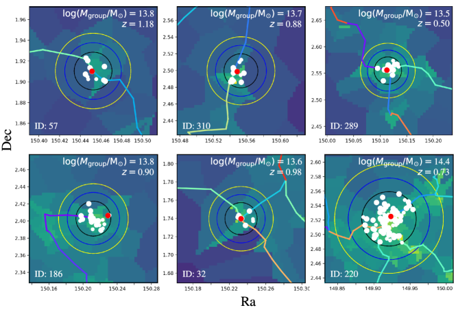
Figure 3: Example of the connectivity of groups of different masses at different redshifts in $\mathscr{C}_{\rm cosmos}$. Each panel is 4 comoving Mpc wide, and the x- and y-axis indicate respectively right ascension and declination. The black, blue and yellow circles are drawn respectively at $1\times$, $1.5\times$ and $2\times$ the virial radius of the group. The connectivity at a given radius is defined as the number of filaments crossing the corresponding circle. Galaxies are represented by white disks. Large and small disks correspond to galaxies more massive and less massive than $10^{10}{\rm M}_{\odot}$ respectively. Only galaxies identified as members of the group and with $\log M_{\rm*}/{\rm M}_{\odot}>9.5$ are shown. The BGG is in red. Distinct filaments have different colours. The background density is estimated from the Delaunay tessellation.

2.2.2 The snapshot catalogue: $\mathscr{C}_{\rm Hzagn\,3D}$

In order to identify galaxies from the stellar particles distribution, we run the AdaptaHOP halo finder (Aubert et al., 2004) on the snapshots. Local stellar particle density is computed from the 20 nearest neighbours, and we keep in the catalogue galaxies with a density threshold equal to 178 times the average matter density at that redshift.

We then extract DM halos from the DM particle distribution following the same procedure as for galaxies, but with a density threshold of 80 times the average matter density. Only halos with more than 100 particles are kept in the catalogue. The centre of the halo is temporarily defined as the densest particle in the halo, and then refined with the shrinking sphere method (Power et al., 2003) in order to recursively find the centre of mass of the halo.

Each galaxy is associated with its closest main halo, and to match the observational definition, the BGG is identified as the most massive galaxy within the virial radius of the main halo. In order to increase the statistics, this group catalogue (called $\mathscr{C}_{\rm Hzagn\,3D}$ in the following) is built by joining the data from three snapshot outputs at $z=0.63,\,0.81,\,1.03$ . This results in 1115 groups with $M_{\rm group}>10^{13}{\rm M}_{\odot}$. In order to get the quenching efficiency for the BGG (Section 4), the galaxy catalogue is matched with its counterpart in the Horizon-noAGN simulation $\mathscr{C}_{\rm Hznoagn\,3D}$. The matching procedure is fully described in Peirani et al. (2017) and Beckmann et al. (2017). The matching procedure identifies 876 groups of $\mathscr{C}_{\rm Hznoagn\,3D}$ which have a counterpart in $\mathscr{C}_{\rm Hznoagn\,3D}$. For these groups, the quenching efficiency due to AGN feedback is defined for matched galaxies as: $\xi=\log(M_{*\,{\rm Hz-noAGN}}/M_{*\,{\rm Hz-AGN}})$. This quenching efficiency is therefore 0 when the galaxy mass is the same in Horizon-AGN and Horizon-noAGN.

TreeMaker (Tweed et al., 2009) is used to build merger trees from the halo catalogues. Each halo in a given snapshot at a given redshift is connected to its main progenitors at higher redshift and its child at lower redshift. Merger trees are built over 38 snapshots in the redshift range $z=\left[0.63,5.87\right]$ corresponding to a time step of about $\sim 200$ Myrs. For each group, we look at its merger history by following back in time its merger tree. The halo is assumed to have encountered a major merger of ratio greater than ($1:x$) if the mass ratio of the second to the main progenitors is greater than $1/x$.

2.2.3 The lightcone catalogues: $\mathscr{C}_{\rm Hzagn\,2D}^{\rm true}$ and $\mathscr{C}_{\rm Hzagn\,2D}^{\rm phot}$

The Horizon-AGN lightcone has been extracted on-the-fly as described in Pichon et al. (2010). Gas cells have been replaced by gas particles, and treated as stars and DM particles. The lightcone projected area is 5 deg² below $z=1$, and 1 deg² above. AdaptaHOP has been run on the lightcone over the redshift range $0<z<4$ with the same method as described above. Photometry is computed for each galaxy in the same filter pass-bands as those available in the COSMOS2015 catalogue, as fully described in Laigle et al. (2019). We simply recall here the main features of this catalogue. For a given galaxy, each of its stellar particles is linked to a single stellar population (SSP) obtained with the stellar population synthesis model of Bruzual & Charlot (2003), with a Chabrier initial mass function (IMF, Chabrier, 2003). The galaxy spectrum is the sum of the contributions of the individual SSP. Dust attenuation is also accounted for. From this virtual photometry, photometric redshifts and masses have been derived with Lephare (Arnouts et al., 2002) with the same configuration as in COSMOS, and the performance of the simulated catalogue is very similar to the observed one in terms of redshift and mass accuracy (Laigle et al., 2019). $\mathscr{C}_{\rm Hzagn\,2D}^{\rm true}$ is the catalogue which makes use of the exact galaxy redshifts and masses, while $\mathscr{C}_{\rm Hzagn\,2D}^{\rm photo}$ uses the photometric redshifts and masses. In order to mimic COSMOS data, we keep only groups more massive than $10^{13.3}{\rm M}_{\odot}$ and containing a BGG more massive than $10^{10}{\rm M}_{\odot}$. We are left with 76 groups over 1 deg², which is slightly more than in COSMOS. However cosmic variance is expected to be quite important on these small fields, and the COSMOS group density should be corrected for the small variation of the group mass limit to be fully comparable to the simulated group density.

2.3 Extraction of filaments and connectivity estimator

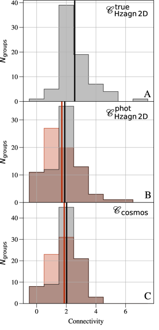
Figure 4: Distribution of group connectivity using a filament extraction based on true-$z$ (panel A) and photo-$z$ (panel B) from the Horizon-AGN simulation. The panel C shows the PDF of the connectivity in the COSMOS dataset. The grey and pink histograms correspond to the distribution with ${\rm 1a}-\pazocal{C}$ groups classed as 2$-\pazocal{C}$ or 1$-\pazocal{C}$ respectively (see text for details). Black and red lines correspond to the mean of the grey and pink histograms respectively.

2.3.1 Extraction of the filaments in 3D

To identify the cosmic network from the density field, we use the persistence based filament tracing algorithm (DisPerSE, Sousbie, 2011), which identifies ridges from the density field as the special lines connecting topologically robust pairs of saddle-peak critical points. Therefore, the extraction is global in the sense that what determines the presence of a filament at a given location is not only the amplitude of the overdensity with respect to the local background, but also the distribution of matter on a larger scale (that is, the presence of a saddle point or a peak further away). In the following, we call “nodes” the maxima of the density field (where filaments are crossing). In Sousbie et al. (2011), DisPerSE was successfully used to extract filaments around an X-Ray detected group at $z=0.083$. For the 3D extraction of the filaments in Horizon-AGN, the density field is reconstructed from the Delaunay tessellation on the entire sample of DM halos (Schaap & van de Weygaert, 2000).

Each filament is defined as a set of connected small segments linking extrema to saddle points. The set of filaments is called the skeleton in the following. Persistence is defined as the difference in density at the two critical points within a pair. Expressed in terms of numbers of $\sigma$, persistence quantifies the significance of the critical pairs in the Delaunay tessellation of a random discrete Poisson distribution. Thus, the filtering of low-persistence structures ensures that the extraction is robust with respect to noise. We choose a 5$\sigma$ persistence threshold to extract filaments in 3D from Horizon-AGN.

2.3.2 Extraction of the filaments in 2D

For the observed catalogue ($\mathscr{C}_{\rm cosmos}$) and the simulated ones from the lightcone ($\mathscr{C}_{\rm Hzagn2D}^{\rm true}$ and $\mathscr{C}_{\rm Hzagn2D}^{\rm phot}$), filaments of the cosmic web are identified from the 2D density field, computed from the Delaunay Tessellation of the galaxy distribution, following Laigle et al. (2018). However, we introduce two changes compared to this previous extraction.

Choice of the slice thickness

We consider slices of a fixed comoving thickness 120 Mpc instead of 75 Mpc (as was chosen in Laigle et al. (2018)). The motivation is to increase the redshift range of the study (up to $z\sim 1.2$ instead of $z\sim 0.9$) while keeping the thickness of the slices calibrated on the typical redshift uncertainty of the lowest mass galaxies in our mass-limited sample ($\Delta_{z}\sim$0.07, that is about 120 cMpc, at $z\sim 1.2$ for $\log M_{*}/{\rm M}_{\odot}\sim 10$). As shown in Laigle et al. (2018), there is no truly optimal slice thickness for extracting filaments (within some range), allowing for a flexible choice without degrading the quality of the extraction. It should in practice primarily be guided by the photometric redshift uncertainties of the lowest mass galaxies in the sample. More specifically, the slice thickness is taken as $2\times$ the $\sigma_{z}$ uncertainty of the 5000 lowest mass galaxies in the redshift and mass bin considered. In order to get a constant slice thickness over the whole redshift range, we calibrate the slice thickness on the lowest mass galaxies at $z\sim 1.2$. As shown in Fig. 2, this implies considering slices of thickness $\sim$120 comoving Mpc. Note that the slice thickness should also be larger than the velocity dispersion in large groups ($\sim 1000$ km/s), which is still small in $\Delta_{z}$ compared to the adopted thickness slices.

The second major change with respect to the analysis in Laigle et al. (2018) concerns the centering of the slices. Because our study is focused on the extraction of filaments around groups, we perform an individual extraction of the filaments for all the groups in our catalogue, each of the groups being put at the center of its own slice. This requirement ensures an optimal extraction of the filaments around all the groups.

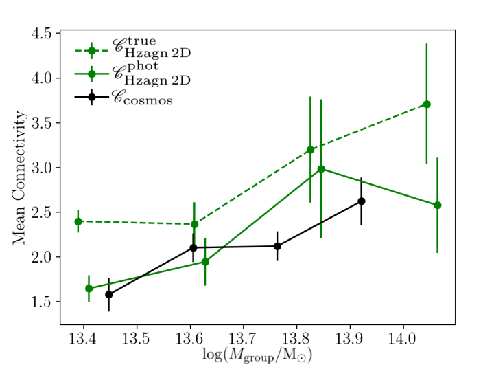
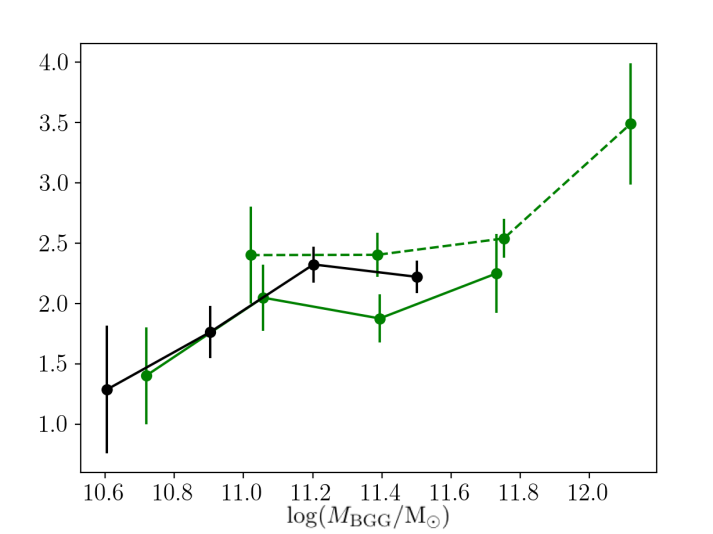
Figure 5: Mean connectivity plotted against group mass $M_{\rm group}$ (left) and BGG mass $M_{\rm BGG}$ (right) for COSMOS data (black line) and the Horizon-AGN simulation (green line) for both photo-z (solid line) and true-z (dashed line) filament extractions. Photometric masses are also used to compute the relation between mean connectivity and BGG mass in the Horizon-AGN mock dataset, which is the reason for the horizontal offset between the solid and dashed curves on the right panel. Errorbars are the error on the mean computed from bootstrap resampling.

Choice of the persistence threshold in 2D

Laigle et al. (2018) chose a persistence threshold of 2$\sigma$ for slice thickness of 75 Mpc at the same mass complenetess as ours. This choice was justified by comparing in mocks the 2D photometric skeleton with the projected 3D one. As shown on their Fig. A.1, minimizing the number of unmatched filaments in the reference and in the reconstructed skeletons implies decreasing the persistence threshold with increasing slice thickness (at a given mass completeness). Therefore, we use in this work a persistence threshold of 1.5$\sigma$ .

2.3.3 Method to measure the connectivity

In the skeleton produced by DisPerSE, two filaments joining the same node can become extremely close to one another, but still counted separately, as they both are topologically robust. However, physically they represent a single filament. Therefore, in order to avoid double counting filaments, they are merged in the final skeleton and a bifurcation point is added at the merging location.
The same ID is then attributed to all segments belonging to the same filaments. Connectivity $\pazocal{C}$ is subsequently defined as the number of segments with different IDs crossing the 1.5$\times$ virial radius circle around the group center. The same definition is taken in 3D and 2D. In appendix A we confirm on the observational dataset that varying this radius does not significantly change the measurement of connectivity and the signal presented hereafter.

Fig. 3 presents six groups in the COSMOS field, with varying masses, redshifts and connectivity, plotted over the underlying density field estimated from the Delaunay Tessellation. Distinct filaments are shown in different colours. The BGG is coloured in red, while the other galaxies in the group are coloured in white. On all these panels, the groups are associated with a peak of the galaxy density distribution, i.e. they are sitting on a node of the cosmic web. The bottom right panel is an example of the highest connectivity found (${4}-\pazocal{C}$, i.e. the group is connected to 4 filaments), while the bottom left panel shows an example of the lowest connectivity found that is still associated with a peak in the distribution (${1}-\pazocal{C}$, i.e. the group is connected to only 1 filament). While a $1-\pazocal{C}$ connectivity is unlikely to happen in theory, this case is found in observations because low persistence filaments were removed from the skeleton. Therefore this group is connected to more filaments, however all but one were too noisy to pass the persistence threshold selection.

2.4 Impact of photo-$z$ errors: insights from mocks

The degradation of the global filament extraction when working with photo-$z$ has already been investigated in Laigle et al. (2018). However we focus here on the degradation of the 2D-connectivity measurement, thanks to the comparison of $\mathscr{C}_{\rm Hzagn2D}^{\rm phot}$ and $\mathscr{C}_{\rm Hzagn2D}^{\rm true}$. The grey histograms on the top and middle panels of Fig. 4 present the PDF of group connectivity from the Horizon-AGN simulation, either using the true galaxy redshift (panel A, $\mathscr{C}_{\rm Hzagn2D}^{\rm true}$) or the photo-$z$ (panel B, $\mathscr{C}_{\rm Hzagn2D}^{\rm phot}$) to extract the 2D cosmic web. The vertical solid black lines give the mean of each distribution. Photo-$z$ errors tend to decrease the global connectivity, as they introduce shot noise in the density measurement and therefore disconnect the field.

In practice, when the measure is performed from photo-$z$ ($\mathscr{C}_{\rm cosmos}$ and $\mathscr{C}_{\rm Hzagn2D}^{\rm phot}$), a non-negligible number of groups are found which are not connected to filaments. Another non-negligible number of groups are embedded in filaments but not associated with a peak of the galaxy density distribution above the persistence threshold (1a$-\pazocal{C}$). Finally, others are associated with a peak of the galaxy distribution, but associated to only 1 filament (1b$-\pazocal{C}$), because the other filaments have been removed when filtering the pairs of critical points below the persistence threshold. These cases are unlikely to occur when connectivity is computed from true galaxy redshifts and are mostly due to noise in the photo-$z$. Indeed, their fractions is almost null in $\mathscr{C}_{\rm Hzagn2D}^{\rm true}$ (top panel), and in particular no 1a$-\pazocal{C}$ case is found.
It is debatable if groups embedded in filaments but not associated with a peak of the density distribution (1a$-\pazocal{C}$) should be counted as 1$-\pazocal{C}$ or 2$-\pazocal{C}$, as there are formally 2 filaments branching out of these groups. The comparative analysis from the detailed mocks suggests these groups should sit at a density peak in the absence of photo-$z$ errors. Therefore in the following we make the choice to consider them as 2$-\pazocal{C}$ (grey histograms on Fig. 4) instead of 1$-\pazocal{C}$ (pink histograms). Appendix A.1 discusses this issue in more details. For each measurement based on $\mathscr{C}_{\rm cosmos}$ presented in the following, we also checked that the result is not strongly dependent on this choice.

Figure 6: The BGG mass against group mass for groups with connectivity smaller than 2 (blue line), connectivity of 2 (red line) and connectivity greater than 2 (yellow line). Two groups of connectivity greater than 2 have their mass higher than 10${}^{14}{\rm M}_{\odot}$. When they are included in the measurement of the last mass bin, we get the yellow triangle marker. The dashed lines correspond to the same measurements, but when classifying the 1a$-\pazocal{C}$ as 1$-\pazocal{C}$ instead of 2$-\pazocal{C}$. The bottom panel shows the distribution of groups in bins of connectivity and group mass. In the corner of each 2D-bin is indicated the number of groups in this bin.

3 Group connectivity in COSMOS

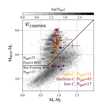
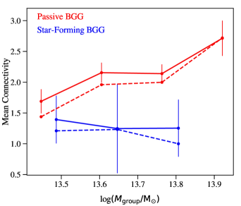
Figure 7: Left: $M_{NUV}-M_{r}$/$M_{r}-M_{J}$ distribution for the entire galaxy population in 0.5$<z<$1.2 and $M_{*}>10^{10}{\rm M}_{\odot}$ in COSMOS (grey area), and for the BGGs only in the same redshift and mass ranges (coloured circles). Circles are coloured according to their connectivity (from low to high connectivity, blue to yellow respectively, according to the binning shown in Fig. 6), and their sizes reflect the group masses. The solid line is the usual separation between passive and star-forming galaxies (see text). For clarity, only errorbars for the low-connectivity BGGs are shown. Right: Mean connectivity as a function of group mass in COSMOS, for groups with a passive BGG (red line) and groups with a star-forming one (blue line). The dashed lines correspond to the same measurements, but when classifying the 1a$-\pazocal{C}$ groups as 1$-\pazocal{C}$ instead of 2$-\pazocal{C}$.

The grey histograms on the middle and bottom panels of Fig. 4 show the distribution of the connectivity in the full redshift range $0.5<z<1.2$ in the Horizon-AGN and COSMOS datasets. We measure $\langle\pazocal{C}\rangle=2.02$ ; ${\rm RMS}\left(\pazocal{C}\right)=0.92$ in $\mathscr{C}_{\rm cosmos}$, $\langle\pazocal{C}\rangle=2.56$ ; ${\rm RMS}\left(\pazocal{C}\right)=1.10$ in $\mathscr{C}_{\rm Hzagn2D}^{\rm true}$ and $\langle\pazocal{C}\rangle=1.89$ ; ${\rm RMS}\left(\pazocal{C}\right)=1.18$ in $\mathscr{C}_{\rm Hzagn2D}^{\rm phot}$.

3.1 Mean connectivity and group mass dependency

The mean group connectivity as a function of group mass can now be measured. In both COSMOS and the Horizon-AGN datasets, the group mass $M_{\rm group}$ is defined as the total mass, i.e. the sum of DM and baryonic mass. The left panel of Fig. 5 displays this measurement in the mock ($\mathscr{C}_{\rm Hzagn2D}^{\rm phot}$ and $\mathscr{C}_{\rm Hzagn2D}^{\rm true}$, green solid and dashed lines resp.) and in COSMOS ($\mathscr{C}_{\rm cosmos}$, black line). Group mass bins are split to contain an approximately equivalent number of groups in each bin. Unsurprisingly and as discussed above, the measurement performed with true-$z$ lies above the one with photo-$z$. The COSMOS and photo-$z$ Horizon-AGN datasets are however in very good agreement. As expected from theoretical predictions (Codis et al., 2018), more massive groups have, on average, a higher connectivity.

3.2 Impact of connectivity on BGG mass assembly

The impact of the connectivity on the mass assembly of the BGG is now investigated. Our purpose is to quantify if there is any correlation between connectivity and the BGG properties (mass and type) beyond the trend driven by the group mass (which scales with connectivity). The adopted strategy is therefore to look at each of these quantities in bins of group mass.

3.2.1 Mass of the BGG

The overall evolution of mean connectivity as a function of BGG mass is first measured. This result is displayed in the right panel of Fig. 5. As a consequence of the assumptions made at the SED-fitting stage when computing masses from photometry (Laigle et al., 2019), the BGG photometric masses are systematically underestimated with respect to their intrinsic mass in Horizon-AGN, which is the reason for the horizontal offset between the solid and dashed green curves. Taking into account this systematic, as well as the lowering of the connectivity when computed from photometric redshifts, brings $\mathscr{C}_{\rm Hzagn2D}^{\rm phot}$ in good agreement with $\mathscr{C}_{\rm cosmos}$ within the errorbars (green and black curves respectively). As expected, the connectivity is higher when the BGG is more massive. At first order this result is a natural consequence of the scaling of group mass with connectivity, given the known correlation between group mass and mass of the BGG.

In order to investigate if there is an additional correlation between connectivity and BGG mass (beyond the effect driven by group mass), the top panel of Fig. 6 presents the BGG mass as a function of group mass in 3 different connectivity bins. The bottom panel presents how groups are distributed within the mass and connectivity bins. Group mass bin are uniformly distributed in logarithm scale between $10^{13.38}{\rm M}_{\odot}$ and $10^{14.02}{\rm M}_{\odot}$. At fixed group mass in the low mass bins ($M_{\rm group}\lesssim 10^{13.7}{\rm M}_{\odot}$), there is a significant trend for the BGG to have higher mass at higher connectivity. In the highest mass bins, the mass of the BGG for groups with $\pazocal{C}\geq 3$ (yellow solid line) is on average lower as those with $\pazocal{C}=2$ (red line). Note that two groups in the highest connectivity bin have their mass higher than $10^{14}{\rm M}_{\odot}$, and are therefore not included by default on the highest mass bin. Including them (yellow triangle marker) in the highest mass bin sensibly biases the mass distribution of groups in this connectivity bin (compared to the medium connectivity bin). In despite of this, the mean BGG mass is still lower than the one in the medium connectivity bin (compare the last red circle marker and the yellow triangle marker). We also checked that this measurement is not strongly dependent on the choice we made to consider 1a$-\pazocal{C}$ groups as 2$-\pazocal{C}$ (compare solid and dashed lines).

Although this result needs more statistics to be confirmed, it suggests that low-mass groups build more efficiently the mass of their BGG at high connectivity, while in high mass group there is a stagnation of the BGG mass assembly at high connectivity. Altogether, this suggests that connectivity might trace different assembly histories of groups.

3.2.2 Type of the BGG

To further probe the link between connectivity and the mass assembly of the BGG, the relationship between connectivity and group mass is investigated in COSMOS by splitting the group population as a function of the type of their BGG. The classification between star-forming and passive galaxies is performed according to the $M_{NUV}-M_{r}$/$M_{r}-M_{J}$ diagram as shown in the left panel of Fig. 7 (as done in Williams et al., 2009; Ilbert et al., 2013; Laigle et al., 2016). Quiescent galaxies are those with $\left[M_{NUV}-M_{r}>3(M_{r}-M_{J})+1\right]\&\left[M_{NUV}-M_{r}>3.1\right]$. Most of the BGG are passive, however 13 of them are classified as star-forming, with group mass ranging from $10^{13.41}{\rm M}_{\odot}$ to $10^{13.89}{\rm M}_{\odot}$. In this mass range, the mean connectivity of groups with a passive BGG is $\langle\pazocal{C}_{\rm pass}\rangle=$2.09, while it is $\langle\pazocal{C}_{\rm sf}\rangle=$1.3 for the groups with a star-forming BGG. In the left panel of Fig. 7, circles representing BGG are color-coded according to the connectivity of their group, and their size scales with the mass of the group. Although some groups with a passive BGG have a low connectivity, no star-forming BGG except one (in the vicinity of the separation line) are in the highest connectivity bin.

As a complement, the right panel of Fig. 7 presents the mean connectivity, as a function of group mass, of groups with either a passive or a star-forming BGG. At a fixed group mass, the mean connectivity of groups with a passive BGG is higher than for groups with a star-forming BGG. This result suggests that higher connectivity implies a higher chance for the BGG to be quenched. The analysis of the Horizon-AGN simulation in the following Section 4 will help interpreting this result.

4 Interpretation and discussion

4.1 Summary of the observational findings

The observational results presented in the previous section confirm first that connectivity scales as a function of group mass. The agreement of this result with theoretical predictions is also indirectly a quality assessment of the filament extraction from photo-$z$ redshift in COSMOS. The relation between BGG mass and connectivity is at first order a natural consequence of the relation between group mass and connectivity.

We also investigated the correlation between connectivity and the properties of the BGG (mass and type) beyond the trend which could be deduced from the correlation between connectivity and group mass. We found that, in low mass groups ($M_{\rm group}\lesssim 10^{13.7}{\rm M}_{\odot}$), the mass of the BGG is on average higher if the connectivity is higher. This trend reverses above this mass, with BGGs in highly connected groups ($\pazocal{C}\geq 3$) being on average less massive than their counterparts in groups of the same mass (Fig. 6). In addition, even if passive galaxies are found both at low and high connectivity, BGGs hosted by highly connected groups are always passive (Fig. 7), suggesting a quenching process connected with (but not necessarily caused by) a high connectivity.

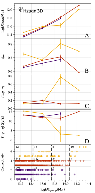
Figure 8: Group properties as a function of group mass in Horizon-AGN, in 3 different connectivity bins. Panel A: mean BGG mass; Panel B: mean quenching efficiency due to AGN feedback; Panel C: fraction of groups with a major merger of ratio (1:2) during the last 6 Gyrs; Panel D: mean time in Gyrs since the last major merger of ratio (1:3). Bottom panel: the distribution of groups in bins of connectivity and group mass. The number of groups in each bin is indicated on the top left of the cell. The groups of a given colour set are used to build the curves of the same colour in the panels $A$, $B$, $C$ and $D$.

Several physical processes might be responsible for this trend. First, assuming gas accretion rate scales with connectivity, one can expect that higher gas infall along more filaments triggers stronger feedback within the BGG. This feedback could in turn prevent stellar mass growth. This interpretation is appealing, as it could both explain the trend at low group mass (higher connectivity groups host more massive galaxies, because more matter is efficiently accreted onto the BGG) and the reverse of this trend at high group mass (the higher accretion rate in high connectivity triggers stronger AGN feedback). These findings might also be an outcome of assembly bias, in which higher connectivity might be a tracer of recent group mergers. As a matter of fact, when two groups of connectivity $n$ and $m$ respectively are merging along a filament, their others filaments are likely to not merge in the same timescale. The net connectivity resulting of the merger will therefore be $n+m-2$. As long as both $n$ and $m$ are greater than 2, the resulting connectivity will be higher than the mean connectivity of the 2 progenitors. Mergers are violent events. The merger of two halos -and consequently their two central galaxies- might shock-heat the gas, but also increase the velocity dispersion, enhance black hole growth and in particular be the reason for stronger AGN feedback (e.g. Di Matteo et al., 2005). Although mergers can temporally trigger bursts of star formation (e.g. Di Matteo et al., 2007; Martin et al., 2017), the merger-enhanced AGN activity can in the long term durably quench the galaxies (e.g. Springel et al., 2005; Dubois et al., 2016). This interpretation from mergers is consistent with previous works finding that SFR is enhanced in isolated groups compared to groups embedded in larger structures (e.g. Scudder et al., 2012, where AGN however have been explicitly excluded from the sample; Luparello et al., 2015).

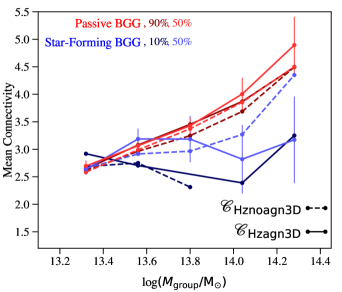
Figure 9: Mean connectivity as a function of group mass in the Horizon-AGN (solid line) and Horizon-noAGN (dashed line) for passive (red) and star-forming (blue) BGGs, while chosen the two extreme thresholds (from dark to light colours) to separate the passive population from the star-forming one (see text for details). For clarity, only errobars on the lighest curves are shown.

4.2 Interpretation from Horizon-AGN

We also conduct complementary measurements in the Horizon-AGN simulation with the $\mathscr{C}_{\rm Hzagn3D}$ catalogue in order to understand the observational results.

Mean connectivity is first measured as a function of group mass both for groups with a passive and star-forming BGG. Separating passive and star-forming BGGs from the $M_{NUV}-M_{r}$/$M_{r}-M_{J}$ diagram is less easy in Horizon-AGN than in COSMOS, as there is residual star-formation even in the passive systems (Kaviraj et al., 2017). For this reason we decided to sort galaxies based on their specific Star-Formation Rate (sSFR) and to define the star-forming sequence as the galaxies with the highest sSFR and the passive sequence as the galaxies with the lowest sSFR (note that the trend does not change when galaxies are sorted according to their SFR rather than their sSFR). Fig. 9 shows the mean connectivity as a function of group mass in $\mathscr{C}_{\rm Hzagn3D}$ (solid line), for the groups with a passive (red lines) and star-forming (blue lines) BGG, while choosing two extreme thresholds (in percentage of the total population) to separate the star-forming from the passive BGGs. Overall, whatever the chosen threshold, a trend qualitatively similar to the observations is found in the simulation: the mean connectivity of groups with a star-forming BGG is lower than the one with a passive BGG, especially at high group mass. However, we note that the typical group mass for which a difference between the mean connectivity of the star-forming and passive populations is measurable ($\log M_{\rm group}>10^{13.8}{\rm M}_{\odot}$) is higher than in $\mathscr{C}_{\rm cosmos}$ ($\log M_{\rm group}>10^{13.5}{\rm M}_{\odot}$). We carry out the same measurement in the simulation without AGN feedback (dashed line) and a weaker trend emerges, suggesting that AGN feedback is important to durably quench the galaxies at high connectivity, but might not be the only driver of the trend.

We turn then to measuring the mean BGG mass as a function of group mass, in bins of connectivity (panel A of Fig. 8). As found in observations, the high-mass groups in the highest connectivity bins tend to have a lower mean BGG mass than those in the intermediate connectivity bins, although the trend is not very significant. We do not find a significant reversal of this trend at low group mass (the fact that more connected groups have a more massive BGG at fixed group mass).
In order to understand the role AGN feedback plays in driving this trend, the mean quenching efficiency due to AGN feedback is also displayed as a function of group mass, in distinct connectivity bins. A strong signal for quenching efficiency to be higher in high connectivity groups is detected (panel B of Fig. 8).
We then measure, in each connectivity bins, the fraction of groups with a recent major merger of ratio greater than ($1:2$) (panel C of Fig. 8). There is a significant signal for this fraction to be higher at higher connectivity. Finally, we measure in bins of group mass the average time spent since the last major merger with a mass ratio greater than ($1:3$) (panel D of Fig. 8). At a given group mass, there is a significant signal for the halos in the highest connectivity bin to have encountered a major merger more recently than in the lower connectivity bins.

Consistently with the observational results at high group mass, our measurements support a scenario in which high connectivity is associated with a stagnation of star formation. In addition, we found higher AGN quenching efficiency at higher connectivity. Furthermore, the groups with the highest connectivity are found to have more likely encountered a major merger recently. These measurements are consistent with a scenario in which mergers might be responsible for populating the high connectivity bin. As mergers favour black hole growth (Hopkins et al., 2008; Schawinski et al., 2010; Dubois et al., 2016) and AGN activity, AGN feedback might be stronger in high connectivity groups and more efficient in quenching the BGG. Further measurements, including the black hole growth and AGN activity, gas inflows and outflows, BGG morphology and redshift evolution of the signal, are still required to fully confirm this scenario. These measurements are beyond the scope of this paper and will be carried out in a upcoming work.

5 Summary and conclusion

The number of filaments connected to a given group (within 1.5 times the virial radius) has been measured in COSMOS around X-Ray detected groups in the redshift range $0.5<z<1.2$. Its correlation with group mass, BGG mass and type has been investigated. The summary of our findings is as follows:

• In COSMOS, groups are found to be connected on average to 2 filaments, and up to 4 filaments. A small fraction of X-ray-detected groups do not lie at a peak of the galaxy distribution as extracted by DisPersE;

• A mock photometric catalogue extracted from the Horizon-AGN lightcone has been used to test the impact of photo-$z$ errors on connectivity. We found that connectivity is systematically underestimated when using photo-$z$ with respect to exact redshifts. Conversely, the distribution of the connectivity in COSMOS and in the virtual mock photometric Horizon-AGN catalogue agree well;

• Group mass and BGG mass increase with increasing group connectivity. This result is measured both in COSMOS and in Horizon-AGN, and is in agreement with our current model of structure formation;

• At fixed group mass, the mass assembly of the BGG also depends on connectivity. Star-forming BGG are only found in groups of low and medium connectivity. At high group mass, groups with higher connectivity have a lower mass BGG than their counterpart with lower connectivity. A consistent result is found in Horizon-AGN. In the simulation, AGN feedback quenching efficiency is higher at higher connectivity. Groups in the highest connectivity bin had on average a major merger more recently than at lower connectivity. Alltogether, these findings suggest that different connectivity values trace different histories of group assembly;

• Given the correlation between group center and projected skeleton nodes, our finding suggest that nodes of the 3D skeleton can also be used to predict the loci of X-ray groups, as originally suggested by Sousbie et al. (2011) for clusters.

These findings are qualitatively consistent both in simulations and observational data (see also Sarron et al., 2019, for consistent measurements in the CFHTLS). They underline the role played by the large-scale environment (as quantified by connectivity) in shaping a diversity of BGG properties. More observations will be needed to make this statement more statistically significant.

In closing, this study is a first step towards understanding the impact of the large-scale environment on group mass assembly. In order to know precisely what is the physical process beyond the measured correlation between connectivity and BGG mass and type, more detailed measurements from hydrodynamical simulations are essential. Upcoming 3D spectroscopic redshift surveys, including 4MOST (de Jong et al., 2012), DESI (DESI Collaboration et al., 2016), PFS (Takada et al., 2014), MSE (McConnachie et al., 2016), provided they allow to extract reliable group catalogues, and photometric redshifts surveys including DES (Rykoff et al., 2016), Euclid (Laureijs et al., 2011), WFIRST (Spergel et al., 2013), LSST (LSST Dark Energy Science Collaboration, 2012), KiDs (de Jong et al., 2013) will also prove crucial to extending this pilot study on larger sample and confirming the impact of large-scale environment on group mass assembly.

Beyond the implication for galaxy formation, cosmology would also benefit from group connectivity measurement as demonstrated by Codis et al. (2018). Although it is not possible to make a strong statement on the Dark Energy equation of state from the COSMOS data, the large-scale coverage of Euclid and LSST should allow such statistics.

.1 Impact of radius choice to measure connectivity

We check that our results do not depend on the chosen radius to measure the connectivity. The left panel of Fig. 10 presents the mean connectivity as a function of group mass when measuring the connectivity within 1, 1.5 or 2$\times$ the virial radius of the group. The solid line corresponds to the measurement chosen in the main text. This Figure illustrates that the measured trend of increasing connectivity with group mass does not strongly depend on the chosen radius.

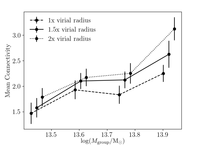
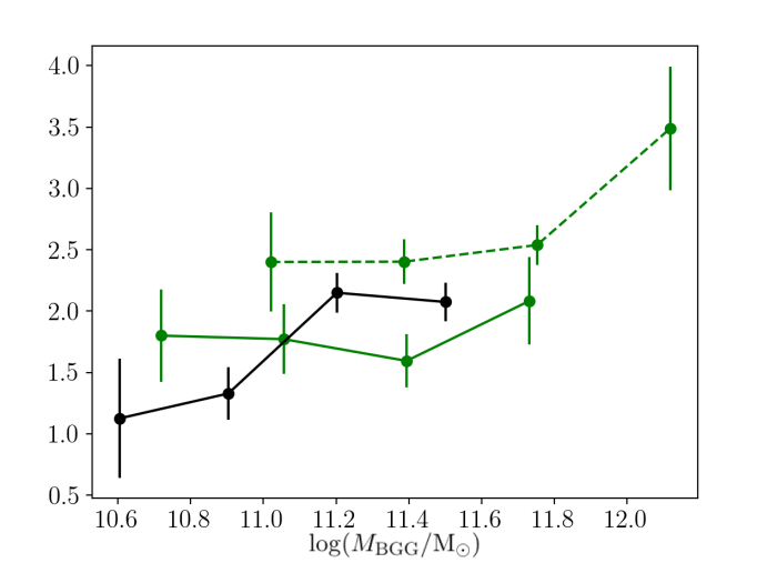
Figure 10: Left: Mean connectivity as a function of group mass, for different radii to measure connectivity in $\mathscr{C}_{\rm cosmos}$. Right: Mean connectivity as a function of BGG mass when counting type-1b connectivity as connectivity 1 (instead of connectivity 2 as done in the main text) for $\mathscr{C}_{\rm cosmos}$ (black line), $\mathscr{C}_{\rm Hzagn2D}^{\rm phot}$ (solid green line), and $\mathscr{C}_{\rm Hzagn2D}^{\rm phot}$ (dashed green line).

Appendix A Counting filaments in COSMOS

A.1 Connectivity 1 versus 2

As discussed in Section 2.4, groups embedded in a filament which do not sit at a peak of the density field (i.e. which are not sitting on a node of the cosmic web) can in principle be assigned a connectivity of either $\pazocal{C}=1$ (1a$-\pazocal{C}$) or $\pazocal{C}=2$. However we also found that photo-$z$ uncertainties tend to decrease connectivity. In other words, the fact that the group does not sit at a peak of the density field might just be due to shot noise driven by photo-$z$ uncertainties. This is confirmed by the fact that 1a$-\pazocal{C}$ is not found when measuring the connectivity from the galaxy distribution with exact redshift. This fact has driven our choice to consider 1a$-\pazocal{C}$ as $2-\pazocal{C}$ in the subsequent measurements.
The right panel of Fig. 10 presents the measurement of mean connectivity versus BGG mass when considering 1a$-\pazocal{C}$ as $1-\pazocal{C}$ (instead of $2-\pazocal{C}$, as was done in the right panel of Figure 5). In this case, the strength of the signal (increase of connectivity for higher BGG masses) decreases when using photo-$z$ (solid line) while it is unchanged when using the intrinsic redshift (dashed line).

References

- Arnouts et al. (2002) Arnouts S., et al., 2002, MNRAS, 329, 355
- Aubert et al. (2004) Aubert D., Pichon C., Colombi S., 2004, MNRAS, 352, 376
- Beckmann et al. (2017) Beckmann R. S., et al., 2017, MNRAS, 472, 949
- Bertin & Arnouts (1996) Bertin E., Arnouts S., 1996, Astronomy and Astrophysics Supplement Series, 117, 393
- Birnboim & Dekel (2003) Birnboim Y., Dekel A., 2003, MNRAS, 345, 349
- Bonjean et al. (2018) Bonjean V., Aghanim N., Salomé P., Douspis M., Beelen A., 2018, A&A, 609, A49
- Bruzual & Charlot (2003) Bruzual G., Charlot S., 2003, MNRAS, 344, 1000
- Byrd & Valtonen (1990) Byrd G., Valtonen M., 1990, ApJ, 350, 89
- Capak et al. (2007) Capak P., et al., 2007, ApJ Sup., 172, 99
- Chabrier (2003) Chabrier G., 2003, PASP, 115, 763
- Codis et al. (2018) Codis S., Pogosyan D., Pichon C., 2018, MNRAS, 479, 973
- Comparat et al. (2015) Comparat J., et al., 2015, A&A, 575, A40
- DESI Collaboration et al. (2016) DESI Collaboration et al., 2016, preprint, (arXiv:1611.00036)
- Danovich et al. (2012) Danovich M., Dekel A., Hahn O., Teyssier R., 2012, MNRAS, 422, 1732
- Danovich et al. (2015) Danovich M., Dekel A., Hahn O., Ceverino D., Primack J., 2015, MNRAS, 449, 2087
- Darvish et al. (2015) Darvish B., Mobasher B., Sobral D., Hemmati S., Nayyeri H., Shivaei I., 2015, ApJ, 814, 84
- Di Matteo et al. (2005) Di Matteo T., Springel V., Hernquist L., 2005, Nature, 433, 604
- Di Matteo et al. (2007) Di Matteo P., Combes F., Melchior A.-L., Semelin B., 2007, A&A, 468, 61
- Dietrich et al. (2005) Dietrich J. P., Schneider P., Clowe D., Romano-Díaz E., Kerp J., 2005, A&A, 440, 453
- Dietrich et al. (2012) Dietrich J. P., Werner N., Clowe D., Finoguenov A., Kitching T., Miller L., Simionescu A., 2012, Nature, 487, 202
- Dubois et al. (2012) Dubois Y., Devriendt J., Slyz A., Teyssier R., 2012, MNRAS, 420, 2662
- Dubois et al. (2013) Dubois Y., Pichon C., Devriendt J., Silk J., Haehnelt M., Kimm T., Slyz A., 2013, MNRAS, 428, 2885
- Dubois et al. (2014) Dubois Y., et al., 2014, MNRAS, 444, 1453
- Dubois et al. (2016) Dubois Y., Peirani S., Pichon C., Devriendt J., Gavazzi R., Welker C., Volonteri M., 2016, MNRAS, 463, 3948
- Durret et al. (2016) Durret F., et al., 2016, A&A, 588, A69
- Finoguenov et al. (2007) Finoguenov A., et al., 2007, ApJ Sup., 172, 182
- George et al. (2011) George M. R., et al., 2011, ApJ, 742, 125
- Gobat et al. (2015) Gobat R., et al., 2015, A&A, 581, A56
- Gouin et al. (2017) Gouin C., Gavazzi R., Codis S., Pichon C., Peirani S., Dubois Y., 2017, A&A, 605, A27
- Gozaliasl et al. (2019) Gozaliasl G., et al., 2019, MNRAS, 483, 3545
- Gunn & Gott (1972) Gunn J. E., Gott III J. R., 1972, ApJ, 176, 1
- Haardt & Madau (1996) Haardt F., Madau P., 1996, ApJ, 461, 20
- Hartley et al. (2015) Hartley W. G., Conselice C. J., Mortlock A., Foucaud S., Simpson C., 2015, MNRAS, 451, 1613
- Hearin et al. (2016) Hearin A. P., Behroozi P. S., van den Bosch F. C., 2016, MNRAS, 461, 2135
- Hopkins et al. (2008) Hopkins P. F., Cox T. J., Kereš D., Hernquist L., 2008, ApJ Sup., 175, 390
- Ilbert et al. (2006) Ilbert O., et al., 2006, A&A, 457, 841
- Ilbert et al. (2009) Ilbert O., et al., 2009, ApJ, 690, 1236
- Ilbert et al. (2013) Ilbert O., McCracken H. J., Le Fevre O., Capak P., Dunlop J., et al. 2013, A&A, 556, A55
- Jauzac et al. (2012) Jauzac M., et al., 2012, MNRAS, 426, 3369
- Jung et al. (2014) Jung I., Lee J., Yi S. K., 2014, ApJ, 794, 74
- Kartaltepe et al. (2010) Kartaltepe J. S., et al., 2010, ApJ, 709, 572
- Kauffmann et al. (2010) Kauffmann G., Li C., Heckman T. M., 2010, MNRAS, 409, 491
- Kauffmann et al. (2013) Kauffmann G., Li C., Zhang W., Weinmann S., 2013, MNRAS, 430, 1447
- Kaviraj et al. (2017) Kaviraj S., et al., 2017, MNRAS, 467, 4739
- Kereš et al. (2005) Kereš D., Katz N., Weinberg D. H., Davé R., 2005, MNRAS, 363, 2
- LSST Dark Energy Science Collaboration (2012) LSST Dark Energy Science Collaboration 2012, preprint, (arXiv:1211.0310)
- Laigle et al. (2016) Laigle C., et al., 2016, ApJ Sup., 224, 24
- Laigle et al. (2018) Laigle C., et al., 2018, MNRAS, 474, 5437
- Laigle et al. (2019) Laigle C., et al., 2019, MNRAS,
- Laureijs et al. (2011) Laureijs R., et al., 2011, preprint, (arXiv:1110.3193)
- Le Fèvre et al. (2015) Le Fèvre O., et al., 2015, A&A, 576, A79
- Leauthaud et al. (2010) Leauthaud A., et al., 2010, ApJ, 709, 97
- Lilly et al. (2007) Lilly S. J., et al., 2007, ApJ Sup., 172, 70
- Luparello et al. (2015) Luparello H. E., Lares M., Paz D., Yaryura C. Y., Lambas D. G., Padilla N., 2015, MNRAS, 448, 1483
- Martin et al. (2017) Martin G., Kaviraj S., Devriendt J. E. G., Dubois Y., Laigle C., Pichon C., 2017, MNRAS, 472, L50
- McConnachie et al. (2016) McConnachie A., Babusiaux C., Balogh M., Driver S., Côté et al. 2016, preprint, (arXiv:1606.00043)
- McCracken et al. (2012) McCracken H. J., et al., 2012, A&A, 544, A156
- Miyazaki et al. (2012) Miyazaki S., et al., 2012, in Society of Photo-Optical Instrumentation Engineers (SPIE) Conference Series. p. 0, doi:10.1117/12.926844
- Moore et al. (1996) Moore B., Katz N., Lake G., Dressler A., Oemler A., 1996, Nature, 379, 613
- Parekh et al. (2017) Parekh V., Durret F., Padmanabh P., Pandge M. B., 2017, MNRAS, 470, 3742
- Peirani et al. (2017) Peirani S., et al., 2017, MNRAS, 472, 2153
- Pichon et al. (2010) Pichon C., Thiébaut E., Prunet S., Benabed K., Colombi S., Sousbie T., Teyssier R., 2010, MNRAS, 401, 705
- Pichon et al. (2011) Pichon C., Pogosyan D., Kimm T., Slyz A., Devriendt J., Dubois Y., 2011, MNRAS, 418, 2493
- Poudel et al. (2017) Poudel A., Heinämäki P., Tempel E., Einasto M., Lietzen H., Nurmi P., 2017, A&A, 597, A86
- Power et al. (2003) Power C., Navarro J. F., Jenkins A., Frenk C. S., White S. D. M., Springel V., Stadel J., Quinn T., 2003, MNRAS, 338, 14
- Pozzetti et al. (2010) Pozzetti L., et al., 2010, A&A, 523, A13
- Rykoff et al. (2016) Rykoff E. S., et al., 2016, ApJ Sup., 224, 1
- Sarron et al. (2019) Sarron F., Adami C., Durret F., Laigle C., 2019, arXiv e-prints,
- Schaap & van de Weygaert (2000) Schaap W. E., van de Weygaert R., 2000, A&A, 363, L29
- Schawinski et al. (2010) Schawinski K., Dowlin N., Thomas D., Urry C. M., Edmondson E., 2010, ApJ Let., 714, L108
- Scoville et al. (2007) Scoville N., et al., 2007, ApJ Sup., 172, 1
- Scudder et al. (2012) Scudder J. M., Ellison S. L., Mendel J. T., 2012, MNRAS, 423, 2690
- Simha et al. (2009) Simha V., Weinberg D. H., Davé R., Gnedin O. Y., Katz N., Kereš D., 2009, MNRAS, 399, 650
- Sousbie (2011) Sousbie T., 2011, MNRAS, 414, 350
- Sousbie et al. (2011) Sousbie T., Pichon C., Kawahara H., 2011, MNRAS, 414, 384
- Spergel et al. (2013) Spergel D., et al., 2013, preprint, (arXiv:1305.5422)
- Springel et al. (2005) Springel V., Di Matteo T., Hernquist L., 2005, ApJ Let., 620, L79
- Sutherland & Dopita (1993) Sutherland R. S., Dopita M. A., 1993, ApJ Sup., 88, 253
- Takada et al. (2014) Takada M., et al., 2014, PASJ, 66, R1
- Taniguchi et al. (2007) Taniguchi Y., et al., 2007, ApJ Sup., 172, 9
- Taniguchi et al. (2015) Taniguchi Y., et al., 2015, PASJ, 67, 104
- Teyssier (2002) Teyssier R., 2002, A&A, 385, 337
- Tillson et al. (2011) Tillson H., Miller L., Devriendt J., 2011, MNRAS, 417, 666
- Treyer et al. (2018) Treyer M., et al., 2018, MNRAS, 477, 2684
- Tweed et al. (2009) Tweed D., Devriendt J., Blaizot J., Colombi S., Slyz A., 2009, A&A, 506, 647
- Weinmann et al. (2006) Weinmann S. M., van den Bosch F. C., Yang X., Mo H. J., 2006, MNRAS, 366, 2
- Williams et al. (2009) Williams R. J., Quadri R. F., Franx M., van Dokkum P., Labbé I., 2009, ApJ, 691, 1879
- Zehavi et al. (2018) Zehavi I., Contreras S., Padilla N., Smith N. J., Baugh C. M., Norberg P., 2018, ApJ, 853, 84
- Zhang et al. (2013) Zhang Y., Dietrich J. P., McKay T. A., Sheldon E. S., Nguyen A. T. Q., 2013, ApJ, 773, 115
- de Jong et al. (2012) de Jong R. S., et al., 2012, in Ground-based and Airborne Instrumentation for Astronomy IV. p. 84460T (arXiv:1206.6885), doi:10.1117/12.926239
- de Jong et al. (2013) de Jong J. T. A., et al., 2013, The Messenger, 154, 44
- van de Voort et al. (2017) van de Voort F., Bahé Y. M., Bower R. G., Correa C. A., Crain R. A., Schaye J., Theuns T., 2017, MNRAS, 466, 3460