Decoherence of nonrelativistic bosonic quantum fields

Abstract

We present a generic Markovian master equation inducing the gradual decoherence of a bosonic quantum field. It leads to the decay of quantum superpositions of field configurations, while leaving the Ehrenfest equations for both the field and the mode-variables invariant. We characterize the decoherence dynamics analytically and numerically, and show that the semiclassical field dynamics is described by a linear Boltzmann equation in the functional phase space of field configurations.

I Introduction

Quantum systems with a large number of interacting constituents can often be effectively described in terms of quantum fields. Examples include degenerate quantum gases and fluids Dalton et al. (2015); Rauer et al. (2018), collective degrees of freedom in strongly correlated solid-state systems Blasone et al. (2011); Preiss et al. (2015), acoustic vibrations in superfluid helium Shkarin et al. (2019); Schmitt (2014); Childress et al. (2017), micromechanical oscillators Riedinger et al. (2018); Ockeloen-Korppi et al. (2018), and closely spaced chains of harmonic oscillators realized, for example, in ion traps Monroe and Kim (2013) and superconducting circuits Ockeloen-Korppi et al. (2016). For such many-body systems a minimal and generic field-theoretic model that appropriately accounts for the decoherence dynamics toward a corresponding classical field theory is desirable.

The loss of quantum coherence and the emergence of classical behavior in systems with a finite number of degrees of freedom have been extensively and successfully studied using the framework of open quantum systems Breuer and Petruccione (2002); Gardiner and Zoller (2014); *GardinerII; *GardinerIII. Understanding these phenomena is of paramount importance for the development of quantum technologies, since their performance is ultimately limited by the coupling to the surrounding environment. Decoherence also plays a central role in probing the physics at the quantum-classical border Joos et al. (1996) as superpositions of increasingly macroscopic and complex objects become experimentally accessible Arndt and Hornberger (2014).

For systems with a large number of interacting constituents the combined decoherence dynamics become quickly intractable on an atomistic level. This calls for a field-theoretic description in terms of collective modes. The open quantum dynamics of fields have so far been formulated assuming a linear coupling with an environment Graham and Haken (1970); Alicki et al. (1986); Calzetta and Hu (1995); Albeverio and Smolyanov (1997); Anglin and Zurek (1996); Dalton et al. (2015). While such schemes are adequate for small fluctuations of the field amplitude, they cannot appropriately describe the decoherence of macroscopic superpositions, since the obtained rates become unrealistically large, growing above all bounds Joos et al. (1996).

In this Rapid Communication we introduce a generic Lindblad master equation for nonrelativistic bosonic fields that describes their gradual decoherence. That is, quantum superpositions of different field configurations quickly decay into a mixture while classical superpositions remain practically unaffected. We show that the semiclassical field dynamics is described by a linear Boltzmann equation in the functional phase space of field configurations, which in the diffusion approximation reduces to a Fokker-Planck equation. The noise term in the master equation is minimal, in the sense that it leaves the Ehrenfest equations for both the field and the mode variables unaffected, while slowly increasing the field energy with a state-independent rate.

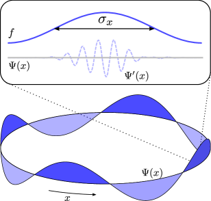
Figure 1: (Color online) The master equation (1) decoheres the state of a bosonic quantum field $\Psi(x)$ by turning quantum superpositions into mixtures. The field dynamics can be viewed as a random process in which the unitary evolution is interrupted by generalized measurements of the canonical field variables whose outcomes are discarded. These fictitious measurements have finite spatial resolution, as characterized by the spread function $f$ of width $\sigma_{x}$.

II Field-theoretic master equation

We consider a bosonic scalar field confined to a one-dimensional region of length $L$, subject to periodic boundary conditions (the generalization to higher dimensions is straightforward). In the Schrödinger picture, its quantum dynamics is described by the master equation

$$\dot{\rho}_{t}=-\frac{\mathrm{i}}{\hbar}[\mathrm{H},\rho_{t}]+\gamma\!\int_{0}^{L}\!\frac{\mathrm{d}x}{L}\!\int\!\mathrm{d}^{2}\xi\,g(\xi)\!\left[\mathrm{U}_{x}(\xi)\rho_{t}\mathrm{U}_{x}^{\dagger}(\xi)-\rho_{t}\right].$$ (1)

The first term describes the unitary dynamics of the field, as determined by the Hamiltonian $\mathrm{H}$, while the second term gives rise to the decoherence of the field. The latter involves unitary phase-space translation operators $\mathrm{U}_{x}(\xi)$ acting on the field amplitude and its canonical conjugate momentum in the vicinity of position $x$. Combining the field variables into the complex field $\Psi(x)$, so that $[\Psi(x),\Psi^{\dagger}(y)]=\delta(x-y)$, these operators can be written as

$$\mathrm{U}_{x}(\xi)=\exp\left(\int_{0}^{L}\mathrm{d}y\,f\left(\frac{y-x}{L}\right)\left[\xi\Psi^{\dagger}(y)-\xi^{\ast}\Psi(y)\right]\right).$$ (2)

Here $f$ is a real, square-integrable, $L$-periodic spread function with maximum $f(0)=1$ and width $\sigma_{x}/L$. The argument $\xi$ of $\mathrm{U}_{x}$ is a complex random number whose associated probability distribution $g(\xi)$ is assumed to be an even function of width $\sigma_{g}$.

From Eq. (1) it follows that the purity $p_{t}=\operatorname{Tr}(\rho_{t}^{2})$ of any quantum state of the field decreases monotonically. To see this we note that $\dot{p}_{t}=2\operatorname{Tr}(\rho_{t}\dot{\rho}_{t})$, and since $\operatorname{Tr}(\rho_{t}[\mathrm{H},\rho_{t}])=0$ and $\operatorname{Tr}\left(\rho_{t}\mathrm{U}_{x}(\xi)\rho_{t}\mathrm{U}^{\dagger}_{x}(\xi)\right)-p_{t}\ =-\frac{1}{2}\left\|\left[\rho_{t},\mathrm{U}_{x}(\xi)\right]\right\|^{2}$, the purity decay rate is given by

$$\dot{p}_{t}=-\gamma\int_{0}^{L}\frac{\mathrm{d}x}{L}\int\mathrm{d}^{2}\xi\,g(\xi)\|[\rho_{t},\mathrm{U}_{x}(\xi)]\|^{2}<0,$$ (3)

where $\|\mathrm{A}\|^{2}=\operatorname{Tr}(\mathrm{A}^{\dagger}\mathrm{A})$. Therefore, the master equation induces the decay of any quantum superposition of the field into a mixture. This loss of coherence will be assessed quantitatively in Sec. IV.

The master equation can be interpreted as describing a compound Poisson process with rate $\gamma$, in which the unitary evolution of the field is interrupted by generalized measurements of the canonical field variables whose outcomes are discarded Kossakowski (1972); Cresser et al. (2006). Whenever a measurement occurs around a position $x\in[0,L]$ it affects an entire neighborhood of width $\sigma_{x}$, as illustrated in Fig. 1. The field degrees of freedom located at any point $y$ within this region experience a random phase-space kick of strength $\xi f(y/L-x/L)$, in accordance with the Heisenberg principle. In the framework of generalized measurements one can thus construct a master equation inducing decoherence without specifying a physical mechanism for the incoherent dynamics, be it the interaction with a practically unobservable environment or, on a more fundamental level, a stochastic process augmenting the Schrödinger equation.

The operators in the master equation can be represented both in position space, in terms of the canonical field amplitude and its conjugate momentum, and in Fourier space, in terms of the mode variables. As will be shown the first representation is advantageous for semiclassical analysis, while the second enables the analytic treatment of the decoherence dynamics.

For definiteness, we take the bosonic field Hamiltonian as

$$\mathrm{H}=\frac{1}{2}\int_{0}^{L}\mathrm{d}x\left[\frac{1}{\mu}\Pi^{2}(x)+\mu\omega^{2}\Phi^{2}(x)+\mu v^{2}[\partial_{x}\Phi(x)]^{2}\right].$$ (4)

The field amplitude $\Phi$ and its canonically conjugate momentum $\Pi$ are related to the complex field through

$$\Psi(x)=\sqrt{\frac{\mu\omega}{2\hbar}}\Phi(x)+\frac{\mathrm{i}}{\sqrt{2\hbar\mu\omega}}\,\Pi(x).$$ (5)

Here $\mu$ is the mass density of the field, $\omega$ is a frequency, and $v$ is a speed.

For example, the Hamiltonian (4) can be used to model the collective dynamics of a chain of many trapped ions (see Ref. Monroe and Kim (2013)). For the continuum description to be valid, the width $\sigma_{x}/L$ of the spread function should be greater than the mean distance between the ions such that the discrete structure of the chain does not get resolved. Likewise, the width $\sigma_{g}$ of the kick distribution must be small enough such that the harmonic approximation remains valid.

The Hamiltonian (4) can be written in diagonal form as $\mathrm{H}=\sum_{k\in K}\hbar\omega_{k}\mathrm{c}_{k}^{\dagger}\mathrm{c}_{k}$, with $\omega_{k}^{2}=\omega^{2}+v^{2}k^{2}$ and $K=\{2\pi j/L\,|\,j\in\mathbb{Z}\}$, thus $k$ runs over all integer multiples of $2\pi/L$. The bosonic mode operators

$$\mathrm{c}_{k}=\sqrt{\frac{\mu\omega_{k}}{2\hbar}}\Phi_{k}+\frac{\mathrm{i}}{\sqrt{2\hbar\mu\omega_{k}}}\,\Pi_{k},$$ (6)

satisfying the canonical commutation relations $[\mathrm{c}_{k},\mathrm{c}^{\dagger}_{k^{\prime}}]=\delta_{kk^{\prime}}$, are defined in terms of the (non-Hermitian) normal coordinates that diagonalize the Hamiltonian (4), $\Phi_{k}=\int_{0}^{L}\mathrm{d}xe^{-\mathrm{i}kx}\Phi(x)/\sqrt{L}$ and $\Pi_{k}=\int_{0}^{L}\mathrm{d}xe^{-\mathrm{i}kx}\Pi(x)/\sqrt{L}$. In the basis (6) the field operators are expressed as

$$\Psi(x)=\frac{1}{\sqrt{L}}\sum_{k\in K}\left[e^{\mathrm{i}kx}\,\Omega^{+}_{k}\mathrm{c}_{k}+e^{-\mathrm{i}kx}\,\Omega^{-}_{k}\mathrm{c}_{k}^{\dagger}\right],$$ (7)

with $\Omega_{k}^{\pm}=[(\omega/\omega_{k})^{1/2}\pm(\omega_{k}/\omega)^{1/2}]/2$.

From a direct calculation using the Baker-Campbell-Hausdorff formula it follows that the mode operators satisfy

$$[\mathrm{H},\operatorname{c}_{k}] = -\hbar\omega_{k}\operatorname{c}_{k},$$ (8a)

$$\,[\operatorname{U}_{x}(\xi),\operatorname{c}_{k}] = -f_{k}e^{-\mathrm{i}kx}(\xi\Omega_{k}^{+}-\xi^{\ast}\Omega_{k}^{-})\operatorname{U}_{x}(\xi),$$ (8b)

where $f_{k}=\int_{0}^{L}\mathrm{d}y\,e^{\mathrm{i}ky}f\left({y}/{L}\right)/\sqrt{L}$ are the Fourier coefficients of $f$. Since $g(\xi)$ is an even function the Ehrenfest equation for the mode operators $\partial_{t}\langle\operatorname{c}_{k}\rangle_{t}=-\mathrm{i}\omega_{k}\langle\operatorname{c}_{k}\rangle_{t}$ is unaffected by the incoherent part of the master equation (1). The expectation values of the field amplitude $\langle\Phi(x)\rangle_{t}$ and its canonical momentum $\langle\Pi(x)\rangle_{t}$ therefore satisfy the field equations associated with the corresponding classical Hamiltonian.

The master equation (1) is most easily solved in the basis of the Weyl operators $\mathrm{D}[\{\eta_{k}\}]=\prod_{k\in K}\exp(\eta_{k}\mathrm{c}_{k}^{\dagger}-\eta_{k}^{\ast}\,\mathrm{c}_{k})$. For each mode variable with wave number $k$, they effect a phase-space displacement by the complex amplitude $\eta_{k}$. In this representation, the state of the field is encoded in the characteristic functional $\chi_{t}[\{\eta_{k}\}]=\operatorname{Tr}(\rho_{t}\mathrm{D}[\{\eta_{k}\}])$.

In the interaction picture with respect to the Hamiltonian (4), henceforth denoted with a tilde, the equation of motion for $\widetilde{\chi}_{t}[\{\eta_{k}\}]$ is given by

$$\partial_{t}\widetilde{\chi}_{t}[\{\eta_{k}\}]=-\Gamma_{t}[\{\eta_{k}\}]\,\widetilde{\chi}_{t}[\{\eta_{k}\}].$$ (9)

This follows from Eq. (1) using the cyclic property of the trace and the canonical commutation relations in Weyl form. For an isotropic $g(\xi)=g_{r}(|\xi|)/2\pi$ the $\xi$ integral is conveniently calculated in polar coordinates. Using the Jacobi-Anger formula for the Bessel function Abramowitz and Stegun (1965) the decoherence rate

$$\Gamma_{t}[\{\eta_{k}\}]=\gamma-\frac{\gamma}{L}\int_{0}^{L}\mathrm{d}x\;\hat{g}_{r}(s_{t}[\{\eta_{k}\},x])$$ (10)

can be written in terms of the Hankel transform of $g$, $\hat{g}_{r}(s)=\int_{0}^{\infty}{\rm d}r\,rg_{r}(r)J_{0}(sr)$, evaluated at

$$s_{t}[\{\eta_{k}\},x]=2\left|\sum_{k\in K}\Omega^{+}_{k}f_{k}e^{\mathrm{i}kx}e^{\mathrm{i}\omega_{k}t}\eta_{k}+\Omega^{-}_{k}f_{k}^{\ast}e^{-\mathrm{i}kx}e^{-\mathrm{i}\omega_{k}t}\eta^{\ast}_{k}\right|.$$ (11)

Equation (9) can be readily solved up to a quadrature. It will be used below to analyze the dynamics of the purity decay. Moreover, it serves as the starting point to derive the semiclassical dynamics of the field. In order to do that, we first reformulate the above results in the language of functional calculus.

III Equation of motion for the Wigner functional

The semiclassical field dynamics induced by Eq. (1) is best described in the phase space of the canonical field variables $\Phi$ and $\Pi$. In this representation, and using the complex field (5), the Weyl operators take the form $\mathrm{D}[\eta]=\exp\left(\int_{0}^{L}\mathrm{d}x\,\left[\eta(x)\Psi^{\dagger}(x)-\eta^{\ast}(x)\Psi(x)\right]\right)$. They are operator-valued functionals effecting a phase-space displacement of the canonical field variables at each point $x$ by the complex wave amplitude $\eta(x)$. [Note that $\eta(x)$ has dimension of reciprocal square root of length, the same as $\Psi(x)$ and $\xi$.]

In this representation, the equation of motion for the characteristic functional takes a form analogous to (9),

$$\partial_{t}\widetilde{\chi}_{t}[\eta]=-\Gamma_{t}[\eta]\,\widetilde{\chi}_{t}[\eta].$$ (12)

Here, the decoherence rate is a functional of the complex wave amplitude $\eta(x)$,

$$\Gamma_{t}[\eta]=\gamma-\frac{\gamma}{L}\int_{0}^{L}\!\mathrm{d}x\int\!\mathrm{d}^{2}\xi\,g(\xi)e^{-\int_{0}^{L}\mathrm{d}y[\eta^{\ast}(y)\Lambda_{t}(\xi,x;y)+\mathrm{c.c.}]}.$$ (13)

It involves the interaction-picture phase-space displacements $\Lambda_{t}(\xi,x;y)=\xi a_{t}(x;y)-\xi^{\ast}b_{t}(x;y)$, with

$$a_{t}(x;y) = \frac{1}{\sqrt{L}}\sum_{k\in K}\left[\cos\omega_{k}t-\frac{\mathrm{i}}{2}\left(\frac{\omega}{\omega_{k}}+\frac{\omega_{k}}{\omega}\right)\sin\omega_{k}t\right]$$ (14a)

$$\times f_{k}e^{\mathrm{i}k(x-y)}$$

$$b_{t}(x;y) = \frac{\mathrm{i}}{2\sqrt{L}}\sum_{k\in K}\!\left(\frac{\omega}{\omega_{k}}-\frac{\omega_{k}}{\omega}\right)\!\sin(\omega_{k}t)f_{k}e^{\mathrm{i}k(x-y)}.$$ (14b)

The Wigner functional of the field state is defined as the functional Fourier transform of $\widetilde{\chi}_{t}[\eta]$

$$\widetilde{W}_{t}[\lambda]=\int{\cal D}^{2}[\eta]\,\widetilde{\chi}_{t}[\eta]\exp\left(\int_{0}^{L}\!\mathrm{d}y\,[\lambda(y)\eta^{\ast}(y)-{\rm c.c}]\right),$$ (15)

where the functional integral is defined as the limit $n\to\infty$ of the corresponding integral over $n$ mode variables Dalton et al. (2015). The equation of motion for the Wigner functional follows from the Fourier transform of (12) as

$$\partial_{t}\widetilde{W}_{t}[\lambda] = -\gamma\,\widetilde{W}_{t}[\lambda]+\frac{\gamma}{L}\!\int_{0}^{L}\!\mathrm{d}x\!\int\!\mathrm{d}^{2}\xi\,g(\xi)\widetilde{W}_{t}[\lambda-\Lambda_{t}(\xi,x)].$$

This equation describes the time evolution of a quasiprobability distribution on a functional phase space. Each point therein is described by a complex function $\lambda(y)$ corresponding to a linear combination of the canonical field variables. The latter are subject to random kicks whose strength is given by the function $\Lambda_{t}(\xi,x;y)$, playing the role of the random variable $\xi f(y/L-x/L)$ in the interaction picture. It thus follows that Eq. (1) can be considered the field-theoretic generalization of a quantum linear Boltzmann equation Vacchini and Hornberger (2009).

We note that in the diffusion limit of small and frequent kicks Eq. (LABEL:eq:Boltzmann-equation) can be approximated by a Fokker-Planck equation Pawula (1967). Expanding the exponential in Eq. (13) to second order in $\xi$ and using that $g(\xi)$ is an even function, the dynamics of $\widetilde{\chi}_{t}[\eta]$ reduces to

$$\partial_{t}\widetilde{\chi}_{t}[\eta]=-\frac{\gamma\sigma_{g}^{2}}{L}\!\int_{0}^{L}\!\mathrm{d}x\left|\int\!\mathrm{d}y\;[\eta(y)a_{t}(x;y)+\eta^{\ast}(y)b_{t}(x;y)]\right|^{2},$$ (17)

where $\sigma^{2}_{g}$ is the second moment of $g$. The functional Fourier transform of (17) can be written in terms of functional derivatives of the Wigner functional using

$$\frac{\delta}{\delta\lambda(y)}\widetilde{W}_{t}[\lambda] = \int\mathcal{D}^{2}[\eta]\,\eta^{\ast}(y)\widetilde{\chi}_{t}[\eta]e^{\int\mathrm{d}z[\lambda(z)\eta^{\ast}(z)-\lambda^{\ast}(z)\eta(z)]},$$

$$\frac{\delta}{\delta\lambda^{\ast}(y)}\widetilde{W}_{t}[\lambda] = -\int\mathcal{D}^{2}[\eta]\,\eta(y)\widetilde{\chi}_{t}[\eta]e^{\int\mathrm{d}z[\lambda(z)\eta^{\ast}(z)-\lambda^{\ast}(z)\eta(z)]},$$

which make use of the identity $\frac{\delta\lambda(z)}{\delta\lambda(y)}=\delta(z-y)$ Zeidler (2007). The resulting equation is

$$\partial_{t}\widetilde{W}_{t}[\lambda] = \int\mathrm{d}x_{1}\mathrm{d}x_{2}\left[Q^{\lambda\lambda}_{t}(x_{2}-x_{1})\frac{\delta}{\delta\lambda(x_{1})}\frac{\delta}{\delta\lambda(x_{2})}\right.$$

$$+Q^{\lambda\lambda^{\ast}}_{t}(x_{2}-x_{1})\frac{\delta}{\delta\lambda(x_{1})}\frac{\delta}{\delta\lambda^{\ast}(x_{2})}$$

$$+Q^{\lambda^{\ast}\lambda}_{t}(x_{2}-x_{1})\frac{\delta}{\delta\lambda^{\ast}(x_{1})}\frac{\delta}{\delta\lambda(x_{2})}$$

$$\left.+Q^{\lambda^{\ast}\lambda^{\ast}}_{t}(x_{2}-x_{1})\frac{\delta}{\delta\lambda^{\ast}(x_{1})}\frac{\delta}{\delta\lambda^{\ast}(x_{2})}\right]\widetilde{W}_{t}[\lambda],$$

with the coefficients

$$Q^{\lambda\lambda}_{t}(x_{2}-x_{1}) = -\gamma\sigma_{g}^{2}\int_{0}^{L}\!\frac{\mathrm{d}x}{L}b_{t}(x;x_{1})a^{\ast}_{t}(x;x_{2}),$$

$$Q^{\lambda\lambda^{\ast}}_{t}(x_{2}-x_{1}) = \gamma\sigma_{g}^{2}\int_{0}^{L}\!\frac{\mathrm{d}x}{L}b_{t}(x;x_{1})b^{\ast}_{t}(x;x_{2}),$$

$$Q^{\lambda^{\ast}\lambda}_{t}(x_{2}-x_{1}) = \gamma\sigma_{g}^{2}\int_{0}^{L}\!\frac{\mathrm{d}x}{L}a_{t}(x;x_{1})a^{\ast}_{t}(x;x_{2}),$$

$$Q^{\lambda^{\ast}\lambda^{\ast}}_{t}(x_{2}-x_{1}) = -\gamma\sigma_{g}^{2}\int_{0}^{L}\!\frac{\mathrm{d}x}{L}a_{t}(x;x_{1})b^{\ast}_{t}(x;x_{2}).$$

Since the Wigner functional (15) is analytic in the complex wave amplitude $\lambda$, the functional derivatives treat $\lambda$ and $\lambda^{\ast}$ as independent variables, like in the Wirtinger calculus Fischer and Lieb (2011). This field-theoretic Fokker-Planck equation can be solved using the techniques introduced in Graham and Haken (1970).

The Wigner representation is also convenient for describing the gradual loss of quantumness induced by the exact Eq. (1). This is because quantum superpositions of macroscopically distinct field states are characterized by a quasiprobability distribution displaying strong oscillations between positive and negative values in a local phase-space region of volume $\hbar$. The decoherence of a superposition due to random phase-space kicks results in the blurring of these fine structures. Once the Wigner functional is nonnegative, it can be viewed as a probability distribution in a functional phase space. The corresponding field state is then indistinguishable from a (mixed) classical field configuration. This loss of coherence will now be quantified through the decay of the purity of the state.

IV Decoherence dynamics

Physically, one would expect that the purity decay rate of a quantum superposition of field states depends on their initial separation as compared to the characteristic width of $g$. Moreover, as we showed in Eq. (3), the purity of a superposition decays monotonically with time. Its functional dependence on the parameters of Eq. (1) is determined by the state of the field. In the following we characterize the dynamics of the purity decay both numerically and analytically for superpositions of single-mode coherent states in the ground mode, $\ket{\psi}=\mathcal{N}(\ket{\alpha}_{0}+\ket{\beta}_{0})\ket{\{0\}_{k\neq 0}}$, with $\mathcal{N}=\left[2+2\,\exp(-\frac{1}{2}|\alpha-\beta|^{2})\cos(2\operatorname{Im}\alpha\beta^{\ast})\right]^{-1}$.

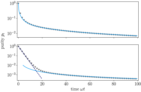
Figure 2: (Color online) Purity decay of a superposition of single-mode coherent states $\ket{\psi}=\mathcal{N}(\ket{\alpha}_{0}+\ket{-\alpha}_{0})\ket{\{0\}_{k\neq 0}}$, with $\alpha=2+2\mathrm{i}$, $v/L\omega=0.01$, and $\sigma_{x}/L=1$. The dots correspond to the exact numerical calculation of Eq. (IV). The top panel shows the case of a narrow kick distribution with $\sigma^{2}_{g}L=0.32$ and for $\gamma/\omega=1$. The solid line is the analytic approximation of Eq. (IV) for $\sigma^{2}_{g}L\ll 1$ and $\sigma_{x}/L\simeq 1$ given in Eq. (24). The opposite case of a broad kick distribution with $\sigma^{2}_{g}L=32$ and for $\gamma/\omega=0.2$ is illustrated in the bottom panel. The solid line gives the long-time behavior obtained using the Laplace approximation, $p_{t}\simeq 1/4\gamma tL\sigma_{g}^{2}$, while the dashed line shows the short-time behavior $p_{t}\simeq\exp(-2\gamma t)$.

The purity of the time-evolved quantum field in the mode representation follows from the solution to Eq. (9),

$$p_{t} = \int{\cal D}^{2}[\{\eta_{k}\}]\,|\chi_{0}[\{\eta_{k}\}]|^{2}\exp\left(-2\int_{0}^{t}\mathrm{d}\tau\Gamma_{\tau}[\{\eta_{k}\}]\right),$$

where $\chi_{0}$ is the characteristic functional of the initial state. For definiteness, we take the kick distribution to be given by

$$g(\xi)=\exp(-|\xi|^{2}/2\sigma_{g}^{2})/2\pi\sigma_{g}^{2},$$ (22)

and choose the spread function $f(s)$ so that

$$f_{k}=\sqrt{L}\exp(-\sigma_{x}^{2}k^{2}/2)/\vartheta_{3}{\bm{(}}0,\exp(-2\pi^{2}\sigma_{x}^{2}/L^{2})\bm{)},$$ (23)

where $\vartheta_{3}$ is the Jacobi theta function Abramowitz and Stegun (1965). In the following we consider a broad spread function with $\sigma_{x}/L\simeq 1$. In this case the approximations $f_{k}\simeq\sqrt{L}\delta_{k,0}$ and $\Gamma_{t}(\{\eta_{k}\})\simeq\gamma-\gamma\exp(-2L\sigma_{g}^{2}|\eta_{0}|^{2})$ can be used.

For the numerical calculation of Eq. (IV) the quantum field is modeled as a harmonic chain of 32 local oscillators. The corresponding phase space is discretized using a generalized Faure sequence L’Ecuyer et al. (2002); Papageorgiou and Traub (1997); Owen (2003).

Figure 2 shows the purity decay for two limiting values of the width of the kick distribution. The initial state is given by $\ket{\psi}=\mathcal{N}(\ket{\alpha}_{0}+\ket{-\alpha}_{0})\ket{\{0\}_{k\neq 0}}$. In the limit of a narrow distribution $g$, such that $\sigma^{2}_{g}L\ll 1$, the purity can be calculated analytically from Eq. (IV),

$$p_{t} \simeq \frac{2\mathcal{N}^{2}}{1+\mu^{2}}\left[1+e^{-\frac{|\alpha-\beta|^{2}}{1+\mu^{2}}}+4e^{-\frac{1}{2}|\alpha-\beta|^{2}}\cos\left(\mathrm{Im}\alpha\beta^{\ast}\right)\right.$$ (24)

$$\left.+e^{-\frac{|\alpha-\beta|^{2}\mu^{2}}{1+\mu^{2}}}+e^{-|\alpha-\beta|^{2}}\cos\left(2\mathrm{Im}\alpha\beta^{\ast}\right)\right],$$

where $\mu^{2}=4\gamma t\sigma_{g}^{2}L$. This expression corresponds to the solid line in the top panel of Fig. 2, which is in excellent agreement with the exact numerical calculation of Eq. (IV). For the case of a broad distribution, $\sigma^{2}_{g}L\gg 1$, the purity cannot be calculated analytically for all times. Its short-time behavior is given by $p_{t}\simeq\exp(-2\gamma t)$, as indicated by the dashed line in the bottom panel, and its long-time evolution can be determined using Laplace’s method Bleistein and Handelsman (1986), yielding $p_{t}\sim 1/4\gamma tL\sigma_{g}^{2}$ as $\gamma t\to\infty$. This asymptotic behavior is indicated by the solid curve in the bottom panel of Fig. 2.

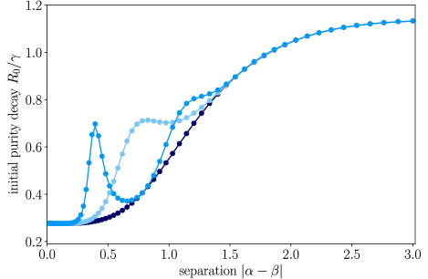
Figure 3: (Color online) Initial purity decay rate, $R_{0}/\gamma$, of a superposition of single-mode coherent states $\ket{\psi}=\mathcal{N}(\ket{\alpha}_{0}+\ket{\beta}_{0})\ket{\{0\}_{k\neq 0}}$ as a function of the separation $|\alpha-\beta|$, for the case $\sigma_{x}/L=1$, with $v/L\omega=0.01$ and $\gamma/\omega=1.0$. The curves show the behavior of $R_{0}/\gamma$ for a narrow kick distribution with $\sigma_{g}^{2}L=0.08$. They correspond to superpositions such that $\alpha+\beta=8,4,0$ (from left to right) with $\alpha-\beta=i|\alpha-\beta|$. The circles give the exact numerical values of Eq. (25), and the solid lines show the analytic approximation of this equation for $\sigma_{x}/L\simeq 1$.

In order to investigate how the purity decay depends on the separation $|\alpha-\beta|$ between the superposed coherent states, we calculate the initial purity decay rate $R_{0}=-\dot{p}_{0}$ from Eq. (IV),

$$R_{0}=2\int{\cal D}^{2}[\{\eta_{k}\}]\,|\chi_{0}[\{\eta_{k}\}]|^{2}\,\Gamma_{0}[\{\eta_{k}\}],$$ (25)

for different initial states. For a broad spread function with $\sigma_{x}/L\simeq 1$ the phase-space integral can be expressed analytically. One finds that $R_{0}-2\gamma$ equals Eq. (24) multiplied by $-2\gamma$, with $\mu^{2}=2\sigma_{g}^{2}L$.

Figure 3 shows that in general $R_{0}$ does not increase monotonically with the separation $|\alpha-\beta|$; it exhibits oscillations for $|\alpha-\beta|<1.5$. Moreover, for large separations the decoherence rate approaches the maximum value

$$\frac{R_{\rm max}}{\gamma}=2-\frac{1}{1+2\sigma^{2}_{g}L}.$$ (26)

In the case of a broad kick distribution $R_{0}$ does not vary appreciably with the separation and approaches the value $R_{\rm max}/\gamma=2$ (not shown). We note that the analytic expression for Eq. (25) (solid curves), calculated assuming $\sigma_{x}/L\simeq 1$, is in excellent agreement with the numerical calculation (circles) of the exact decay rate $R_{0}$.

V Mean energy increase

In addition to inducing decoherence, a quantum master equation will in general also affect the dynamics of otherwise conserved quantities such as energy Bassi et al. (2013). Experimental bounds on the observed conservation of energy will therefore constrain the parameters entering the non-unitary time evolution.

From the master equation (1) it follows that the field energy increases with a constant rate that is independent of the quantum state of the field,

$$\partial_{t}\left\langle\mathrm{H}\right\rangle_{t}=\gamma\sum_{k\in K}\hbar\omega_{k}|f_{k}|^{2}\int\mathrm{d}^{2}\xi\,g(\xi)|\xi\Omega^{+}_{k}-\xi^{\ast}\Omega^{-}_{k}|^{2}.$$ (27)

This is obtained by using the exact expansion $e^{-\mathrm{X}}\mathrm{H}e^{\mathrm{X}}=\mathrm{H}-\left[\mathrm{X},\mathrm{H}\right]+\frac{1}{2}\left[\mathrm{X},\left[\mathrm{X},\mathrm{H}\right]\right]$, where $\mathrm{X}$ is the exponent in Eq. (2).

In the limit of large $L$ the sum over $k$ can be approximated as an integral and the heating rate has the explicit expression

$$\partial_{t}\left\langle\mathrm{H}\right\rangle_{t}=2\sqrt{\pi}\gamma\hbar\omega\sigma_{x}\sigma_{g}^{2}\left(1+\frac{v^{2}}{(2\sigma_{x}\omega)^{2}}\right),$$ (28)

where we used the distribution (22) and the spread function (23).

VI Conclusions

We introduced a generic Lindblad master equation that serves to decohere a nonrelativistic bosonic field. The Ehrenfest equations for the canonical field variables remain identical with the corresponding classical field equations, while quantum superpositions of distinct field configurations are rapidly turned into mixtures. In fact, the master equation induces a monotonic decay of the purity.

We showed that the Wigner functional is an appropriate representation to capture the gradual quantum-to-classical transition of the field. To the extent to which the functional turns positive, its dynamics can be regarded as being governed by a linear Boltzmann equation, which in the diffusion limit reduces to a Fokker-Planck equation. Using the characteristic functional, the decoherence rate of a quantum superposition of two effectively classical field configurations was shown to depend nontrivially on their phase-space separation, and to saturate for large separations.

The effect of the master equation on the field may be viewed as arising from a stochastic process of generalized simultaneous measurements of the field amplitude and its canonical momentum, whose outcomes are discarded. These fictitious measurements have finite spatial resolution, as characterized by the spread function $f$. It is important to remark that only due to the finite width $\sigma_{x}>0$ of $f$ in position space is the continuous field dynamics physically consistent and divergence-free. Moreover, the limited resolution $\sigma_{g}>0$ associated with the generalized measurement of the phase-space coordinates ensures a finite back-action on all canonical field variables.

Notwithstanding the generality of the master equation and its complex decoherence dynamics, several analytical expressions were obtained for functionals of the field state. In particular, we obtained the functional dependence of the purity in the most important limiting cases, and we calculated the exact energy increase. The analytical results are in remarkable agreement with numerical calculations. This shows that for a superposition of field coherent states expectation values can be accurately calculated using quasi Monte Carlo integration based on generalized Faure sequences, despite the high-dimensional character of the phase space.

We note that in Ref. Shimizu and Miyadera (2002) the stability of the quantum state of a macroscopic number of degrees of freedom against perturbation by a quantum or a classical noise was analyzed based on general considerations. Since the present work introduces a concrete decoherence model, it should encourage further investigations of macroscopic quantum systems described by quantum fields.

The methods discussed in this work can be straightforwardly generalized to non-relativistic bosonic tensor fields. In principle, a similar treatment can be developed for fermionic fields, even though their classical analog is less evident. Finally, a relativistic generalization of the model presented here would enable the study of the quantum-to-classical transition of quantum electrodynamics.

M.B. acknowledges financial support from CONACYT (Mexico) and DAAD (Germany).

References

- Dalton et al. (2015) B. Dalton, J. Jeffers, and S. Barnett, Phase Space Methods for Degenerate Quantum Gases (Oxford University Press, 2015).
- Rauer et al. (2018) B. Rauer, S. Erne, T. Schweigler, F. Cataldini, M. Tajik, and J. Schmiedmayer, Science 360, 307 (2018).
- Blasone et al. (2011) M. Blasone, P. Jizba, and G. Vitiello, Quantum Field Theory and Its Macroscopic Manifestations: Boson Condensation, Ordered Patterns, and Topological Defects (Imperial College Press, 2011).
- Preiss et al. (2015) P. M. Preiss, R. Ma, M. E. Tai, A. Lukin, M. Rispoli, P. Zupancic, Y. Lahini, R. Islam, and M. Greiner, Science 347, 1229 (2015).
- Shkarin et al. (2019) A. B. Shkarin, A. D. Kashkanova, C. D. Brown, S. Garcia, K. Ott, J. Reichel, and J. G. E. Harris, Phys. Rev. Lett. 122, 153601 (2019).
- Schmitt (2014) A. Schmitt, Introduction to Superfluidity: Field-theoretical Approach and Applications (Springer International Publishing, Switzerland, 2015).
- Childress et al. (2017) L. Childress, M. P. Schmidt, A. D. Kashkanova, C. D. Brown, G. I. Harris, A. Aiello, F. Marquardt, and J. G. E. Harris, Phys. Rev. A 96, 063842 (2017).
- Riedinger et al. (2018) R. Riedinger, A. Wallucks, I. Marinković, C. Löschnauer, M. Aspelmeyer, S. Hong, and S. Gröblacher, Nature 556, 473 (2018).
- Ockeloen-Korppi et al. (2018) C. Ockeloen-Korppi, E. Damskägg, J.-M. Pirkkalainen, M. Asjad, A. Clerk, F. Massel, M. Woolley, and M. Sillanpää, Nature 556, 478 (2018).
- Monroe and Kim (2013) C. Monroe and J. Kim, Science 339, 1164 (2013).
- Ockeloen-Korppi et al. (2016) C. F. Ockeloen-Korppi, E. Damskägg, J.-M. Pirkkalainen, A. A. Clerk, M. J. Woolley, and M. A. Sillanpää, Phys. Rev. Lett. 117, 140401 (2016).
- Breuer and Petruccione (2002) H.-P. Breuer and F. Petruccione, The Theory of Open Quantum Systems (Oxford University Press, 2002).
- Gardiner and Zoller (2014) C. Gardiner and P. Zoller, The Quantum World of Ultra-Cold Atoms and Light Book I (Imperial College Press, 2014).
- Gardiner and Zoller (2015) C. Gardiner and P. Zoller, The Quantum World of Ultra-Cold Atoms and Light Book II (Imperial College Press, 2015).
- Gardiner and Zoller (2017) C. Gardiner and P. Zoller, The Quantum World of Ultra-Cold Atoms and Light Book III (Imperial College Press, 2017).
- Joos et al. (1996) E. Joos, H.-D. Zeh, C. Kiefer, D. Giulini, J. Kupsch, and I. Stamatescu, Decoherence and the Appearance of a Classical World in Quantum Theory (Springer-Verlag Berlin Heidelberg, 1996).
- Arndt and Hornberger (2014) M. Arndt and K. Hornberger, Nat. Phys. 10, 271 (2014).
- Graham and Haken (1970) R. Graham and H. Haken, Z. Phys. A: Hadrons Nucl. 234, 193 (1970).
- Alicki et al. (1986) R. Alicki, M. Fannes, and A. Verbeure, J. Phys. A: Math. Gen. 19, 919 (1986).
- Calzetta and Hu (1995) E. Calzetta and B. L. Hu, Phys. Rev. D 52, 6770 (1995).
- Albeverio and Smolyanov (1997) S. Albeverio and O. G. Smolyanov, Russ. Math. Surv. 52, 822 (1997).
- Anglin and Zurek (1996) J. R. Anglin and W. H. Zurek, Phys. Rev. D 53, 7327 (1996).
- Kossakowski (1972) A. Kossakowski, Rep. Math. Phys. 3, 247 (1972).
- Cresser et al. (2006) J. D. Cresser, S. M. Barnett, J. Jeffers, and D. T. Pegg, Opt. Commun. 264, 352 (2006).
- Abramowitz and Stegun (1965) M. Abramowitz and I. Stegun, Handbook of Mathematical Functions: With Formulas, Graphs, and Mathematical Tables (Dover Publications, 1965).
- Vacchini and Hornberger (2009) B. Vacchini and K. Hornberger, Phys. Rep. 478, 71 (2009).
- Pawula (1967) R. F. Pawula, Phys. Rev. 162, 186 (1967).
- Zeidler (2007) E. Zeidler, Quantum Field Theory I: Basics in Mathematics and Physics (Springer-Verlag Berlin, 2006).
- Fischer and Lieb (2011) W. Fischer and I. Lieb, A Course in Complex Analysis: From Basic Results to Advanced Topics (Vieweg+Teubner Verlag, 2011).
- L’Ecuyer et al. (2002) P. L’Ecuyer, L. Meliani, and J. Vaucher, in Proceedings of the 2002 Winter Simulation Conference, edited by E. Yücesan, C.-H. Chen, J. L. Snowdon, and J. M. Charnes (IEEE Press, 2002) pp. 234–242, available at http://simul.iro.umontreal.ca/ssj/indexe.html.
- Papageorgiou and Traub (1997) A. Papageorgiou and J. F. Traub, Comput. Phys. 11, 574 (1997).
- Owen (2003) A. B. Owen, ACM Trans. Model. Comput. Simul. 13, 363 (2003).
- Bleistein and Handelsman (1986) N. Bleistein and R. Handelsman, Asymptotic Expansions of Integrals (Dover Publications, 1986).
- Bassi et al. (2013) A. Bassi, K. Lochan, S. Satin, T. P. Singh, and H. Ulbricht, Rev. Mod. Phys. 85, 471 (2013).
- Shimizu and Miyadera (2002) A. Shimizu and T. Miyadera, Phys. Rev. Lett. 89, 270403 (2002).